The Impact of Agriculture on Greenhouse Gas Emissions in the Visegrad Group Countries after the World Economic Crisis of 2008. Comparative Study of the Researched Countries

Abstract

The aim of this study is to identify the correlation between the amount of greenhouse gas emissions, added value from agriculture and economic growth in the Visegrad Group countries. Four countries of Central Europe were studied the Czech Republic, Hungary, Poland and Slovakia in 2008–2019. Due to the objectives of the article, it was decided to use the panel model. The temporal scope of the research covers the years 2008–2019, i.e., two economic periods: 2008–2014 (a downward trend, including agriculture), and 2015–2019 (an upward trend). Greenhouse gas emissions are positively correlated with value added from agriculture and economic growth. The increase in the level of these variables stimulates of the amount of greenhouse gas emissions in the countries of the Visegrad Group. The analysis of the eco-efficiency of greenhouse gas emissions in agriculture, in relation to the gross added value produced, shows that the country with the least pollution of this value was Hungary, followed by Slovakia. The Czech Republic was third, and Poland was the last. The results of the research can be treated as a premise for a strategy for the development of agriculture, limiting the negative effects of its industrial development for more sustainable development.

1. Introduction

Agriculture is a major contributor to anthropogenic global warming, and reducing emissions from agriculture—mainly methane and nitrous oxide—can play a significant role in mitigating climate change [1]. Greenhouse gas emissions in the EU in 2019, according to the European Environment Agency (EEA), were related to such sectors of the economy (excluding LULUCF (land use, land use change and forestry), i.e., a sector that, apart from emissions, can also remove CO₂ from the atmosphere) such as, on the one hand, agriculture (10.55%), on the other hand energy production (77.02%, including about one-third for transport), industrial processes and product consumption (9.11%), while other emissions are accounted for by waste management (3.32%) [2]. The growing concentration of greenhouse gases in the atmosphere, resulting from the activities of industry sectors, affects climate change. According to the IPCC Report (the Intergovernmental Panel on Climate Change), climate change, apart from the increase in temperature, causes many different effects in different regions, which will continue to intensify. Among them, these climate changes, which intensify the water cycle, affect rainfall patterns, and in cities some of these changes may be amplified, including heat, flooding from heavy rainfall, and rising sea levels in coastal cities [3,4]. Agriculture is the main source of two greenhouse gas emissions, methane and nitrous oxide. The emission sources include: enteric fermentation (CH₄), animal feces (CH₄, N₂O), agricultural soils (N₂O emissions from fertilization) and combustion of plant residues (CH₄, N₂O). Currently, efforts are being made to reduce greenhouse gas emissions, as even small emissions significantly affect the Earth’s energy balance. Food of animal origin is more harmful to the climate than the production of food based on plants, which has a much lower environmental impact than food of animal origin. It should also be noted that agriculture causes environmental pollution but is also not indifferent to all pollution caused by greenhouse gas emissions. Climate change is a globally recognized problem that affects both social development and the environment [5]. Mitigating them is a major concern for environmental policymakers [6].

Research in the field of greenhouse gas emissions is complex and multilaterally conditioned. In the literature, we find many references both to the emission efficiency in various countries, determinants influencing the increase in greenhouse gas emissions, or the effects of greenhouse gas emissions in selected sectors of the economy [7,8,9,10,11,12,13,14,15], and to the policy of reducing greenhouse gas emissions [4]. The research is also aimed at monitoring and valuing aggregate emissions of selected greenhouse gases throughout the economy, as and in agriculture [16], and measurements of greenhouse gas emissions are also carried out in order to improve emission factors, identify and promote practices mitigating their effects and conduct emission policies GHG (greenhouse gas) in agriculture [17], as well as assess the impact of agriculture and energy production on the environment through CO₂ emissions [18,19,20,21]. Undoubtedly, understanding the root causes of greenhouse gas emissions in different countries is fundamental to mitigating climate change [7].

The article is structured as follows. Section 2 contains the literature review which was performed to identify of background of the research, Section 3 introduces the proposed materials and methods and Section 4 presents results. In the following Section 5, discussion of results is performed. Section 6 contains the conclusions and policy implications.

2. The Literature Review

Rokicki, Koszela, Ochnio, Golonko, Zak, E.K. Szczepaniuk, H. Szczepaniuk, and Perkowska [10] studied the relationship between greenhouse gas emissions by agriculture and economic development and agricultural production parameters in the European Union in 2004–2017. The research allows [10] that greenhouse gas emissions from agriculture slightly decreased across the EU in 2004–2017. The changes, however, varied. Greenhouse gas emissions from agriculture increased in developing countries, while they remained at a similar level in developed countries. In their study, Perrier, Guivarch and Boucher [9] quantified the contribution of various factors influencing the reduction of emissions in Europe in 2009–2014. They build a novel dataset of deflated input–output tables for each of the 28 EU countries [9], which made it possible to carry out the Analysis of the Structural Distribution of Emissions in European Countries since the Economic Crisis. The Structural Decomposition Analysis was used by Alkan and Oğuş-Binatlı [22] to determine the factors behind the continuously increasing CO₂ emissions in Turkey. They identified the main contributors to CO₂ emissions change within five-year intervals during 1990–2015 by adopting the Structural Decomposition Analysis method. The results show that the CO₂ emissions increase was driven by per capita expenditure and population factors, while the emission coefficient factor had a reducing effect on emissions. Both studies by Rokicki, Koszela, Ochnio, Golonko, Zak, E.K. Szczepaniuk, H. Szczepaniuk, Perkowska [10] and Alkan and Oğuş-Binatlı [22] used the method of structural distribution analysis, which, due to the goals of our research, is insufficiently diagnostic. Hence, we chose panel methods due to, firstly: the possibility of using more data, which is important in the conditions of a limited material–spatial scope of research; secondly, wider operationalization of data and taking into account the individual effects under study; thirdly, identification of the causes of the analyzed phenomena and their dynamics on a micro level. Likewise, Liobikienė and Butkus [6], González-Sánchez and Martín-Ortega [7], identify determinants influencing the increase in greenhouse gas emissions. Other considerations indicate the impact of the common EU policy on greenhouse gas emissions. This aspect was emphasized by Constantin, Radulescu, Andrei, Chivu, Erokhin, and Gao [15] when analyzing the evolution of agriculture in the context of the Common Agricultural Policy from the perspective of sectoral structural changes. They were determined by environmental requirements and work efficiency, which resulted from the application of the cross-sectional linear regression method [15]. We partially use it in our paper, as part of the panel analysis, but due to the limitations of the observation matrix (the considerations concern the Visegrad Group and relevant comparisons), we do not do it to the full extent. However, in order to be able to determine, as mentioned earlier, the correlation between greenhouse gas emissions, added value in agriculture and economic development, it is important to distinguish two economic periods: 2008–2014 (a downward trend in the general profitability index, including agriculture), and 2015–2019 (an upward trend in the general profitability index, including agriculture). We perform this in order to fill the research gap, but also to look again at the variables and their interdependencies. The countries of the Visegrad Group, i.e., Poland, the Czech Republic, Hungary and Slovakia, were selected for the study due to their progressing economic and political integration, but under the conditions of a significantly different history of the development of their agriculture. It should be emphasized that in Poland after World War II, the processes of collectivization and concentration in agriculture were limited in contrast to the other countries surveyed. Another important question was whether this fact was reflected in the currently observed interdependencies between the increase in value added in agriculture (agricultural income) and the overall economic growth and greenhouse gas emissions. Poland, as the only country from the studied group, retained private ownership of farms after World War II, while in other countries, state-owned and collectivized farms dominated in agriculture. In the 1990s, there was a fundamental change in the restoration of the private form of farms in all countries of the Visegrad Group. In Poland, small and medium-area farms were preserved; in other countries the private form of large-area farms was reconstructed. Significant differences between the studied countries that should be taken into account are the different sources of energy obtained. In the case of Poland, energy comes mainly from fossil sources, in Slovakia the production of energy generated from nuclear sources dominates, and in the Czech Republic the dominant source of energy is fossil fuels, including lignite and gas. In Hungary, however, most electricity comes from nuclear power plants and natural gas-fired units. It is worth emphasizing here that agriculture is not only an energy consumer and an emitter of greenhouse gases, but also has the potential to generate renewable energy.

In the literature on the subject, we find many references to the countries of the Visegrad Group. Dzikuć, Wyrobek, and Popławski [23] identified and explained the problems connected with low-carbon development. The purpose of their analyses was also to prove the negative impact of the emission of greenhouse gas emission and other harmful substances into the air on the quality of human life and the natural environment. During the research, they also assessed the eco-efficiency of the used energy resources. In the literature, we also found works on the sphere of agriculture in the Visegrad Group without identifying problems related to greenhouse gas emissions [24,25], as well as works on the analysis of the possibilities of implementing the Paris Agreement and provisions on the goals of reducing greenhouse gas emissions in the EU by Poland, the Czech Republic, Hungary and Slovakia, i.e., countries of the Visegrad Group [26]. The literature also includes works on the premises of bioeconomy development in selected EU countries depending on their general level of economic development. The research concerns four highly developed countries, i.e., Germany, France, Finland and Denmark, and four medium developed countries, i.e., Poland, Hungary, the Czech Republic and Slovakia in 2001–2018 [27].

When determining greenhouse gas emissions from agriculture, we make assumptions that [28]:

• Activity at farm level, although a significant contributor to GHG emissions from agriculture, is usually linked to other economic activity in the region and beyond.
• Most of the agricultural lands are used for commercial farming activities, which also have an impact on greenhouse gas emissions, which broadens the spectrum of the research.
• Reduction of greenhouse gas emissions requires involvement of significant human resources, changes in legal regulations, increased financial outlays as well as organizational and technical changes [29].

3. Materials and Methods

The purpose of this article is to identify the correlation between the amount of greenhouse gas emissions, added value from agriculture and economic growth in the Visegrad Group countries, described by answers to the three research questions:

(1)

Was the world economic crisis of 2008–2009 marked by changes in the amount of greenhouse gas emissions in agriculture in the surveyed countries (Visegrad Group) and did the recovery from this crisis have an impact on gas emissions in their agriculture?

(2)

Are there any differences in the amount of greenhouse gas emissions in the studied countries or, on the contrary, have they been reduced?

(3)

Do the research results allow us to believe that the global economic crisis can be treated as a kind of a warning for a negative increase in the “carbon footprint” and the above-mentioned pollutants in the agriculture of these countries, or vice versa?

The answer to these questions will allow to verify the adopted research hypotheses:

Hypothesis 1 (H1).

There are significant correlations between the amount of greenhouse gas emissions, added value from agriculture and economic growth in the Visegrad Group countries.

Hypothesis 2 (H2).

The world economic crisis of 2008–2009 successively influenced the changes in the accumulation of greenhouse gases, resulting in the reduction of their emissions in the countries of the Visegrad Group.

Hypothesis 3 (H3).

Overcoming the above-mentioned crisis had a positive impact on the level of greenhouse gas emissions in agriculture in the researched countries and can be treated as a premise for the development of agriculture limiting the negative effects of industrial development.

The temporal scope of the research covers the years 2008–2019, i.e., two economic periods: 2008–2014 (a downward trend in the general profitability index, including agriculture), and 2015–2019 (an upward trend in the general profitability index, including agriculture). The spatial scope covers four Central European countries, i.e., Visegrad Group: Czech Republic, Hungary, Poland and Slovakia. In the empirical analysis, a panel model was used, which will be presented in the empirical part of the article.

This chapter is divided into two sections. The first concerns the algorithm of the research procedure (Figure 1), and the second shows greenhouse gas emissions in agriculture under the conditions of its development in the countries of the Visegrad Group.

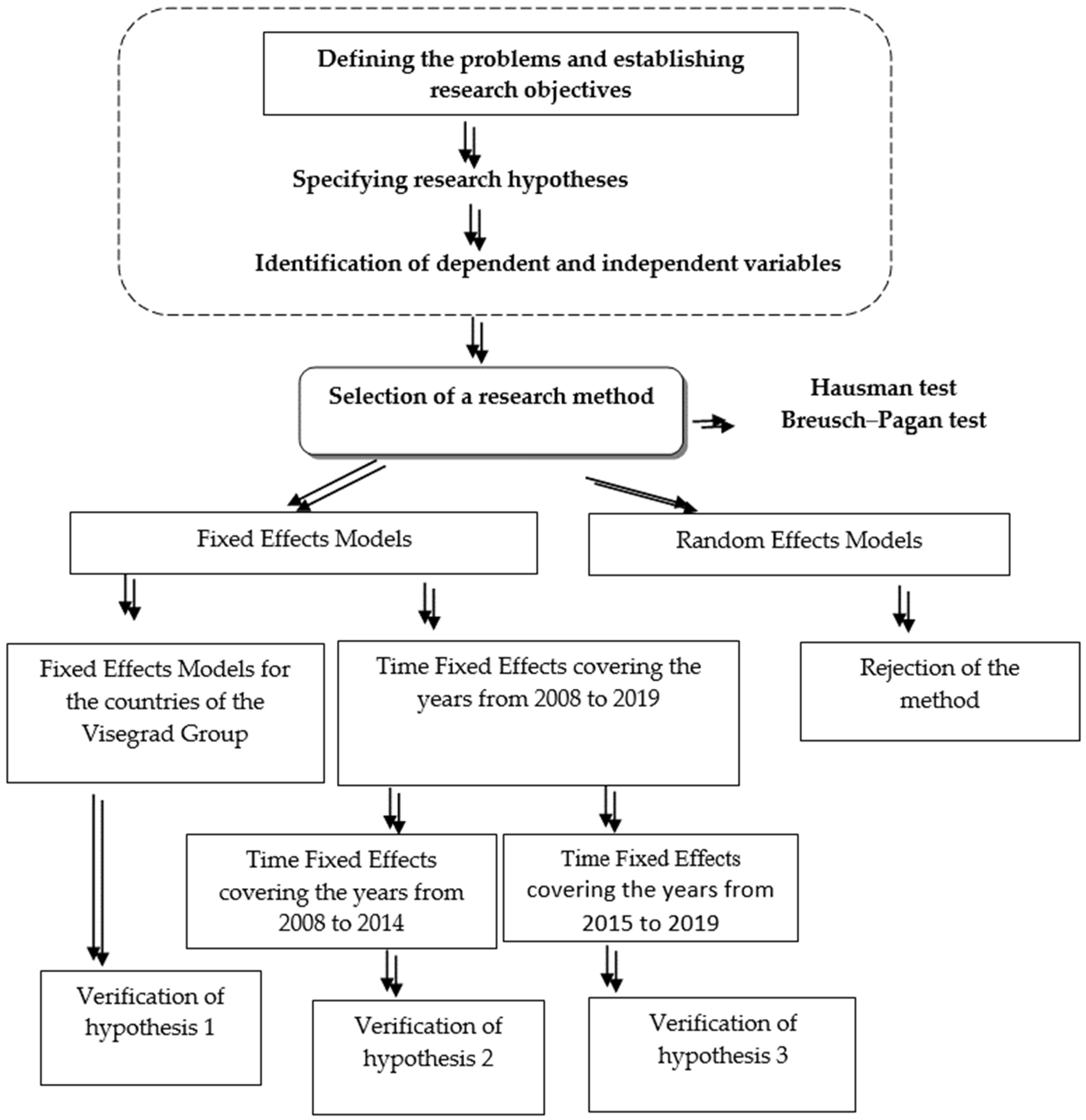
3.1. Steps of Constructing a Reaserch Procedurę and Flowchart of Constructing a Panel Regression Model

As Zhang and Hong [30] have remarked “with economic development, people expect a higher quality of life”. Therefore, it becomes important to create a model based on precise statistical theories and historical data, which will be used to extract the relationships between the relevant variables, all in order to get to know a wider context of the phenomena of interest to the researcher [30]. Figure 1 shows the stages of constructing the research procedure and the scheme of building a regression model of panels.

The individual stages of the research algorithm are interrelated. The first three stages concern the definition of research problems and determination of research goals, followed by the formulation of research hypotheses and the identification of variables. Next, regarding the choice of research method, a panel model was taken into account in the study. In the research process, the method used was verified with the Hausman [31] and Breusch–Pagan tests [32]. The next stages show the phase of the research implementation, in which the adopted research hypotheses are verified.

3.2. Greenhouse Gas Emissions in Agriculture in Terms of Its Development in the Countries of the Visegrad Group

Taking into account greenhouse gas emissions in agriculture and its development in the Visegrad Group countries, it should be noticed that the development is illustrated by two variables. On the one hand, gross value added to agriculture together with forestry and fishery, and on the other hand, gross value added to production sectors of the economy (except agriculture), including industry, construction, trade, transport, communications and other service activities, which has been analyzed [25]. In the article, we assume that the selection of a synthetic (holistic) variable, which is gross value added in the production sectors of the Visegrad Group economies (except agriculture), is related to their impact on the conditions of agricultural production, resulting from environmental and climate changes caused by the emissions of greenhouse gases.

Let us examine the emissions in individual countries of the Visegrad Group. According to Eurostat data [33], in 2019 the total greenhouse gas emissions from agriculture, calculated in CO₂ equivalent, excluding the emission and removal of greenhouse gases from LULUCF, in Poland amounted to 32,735.41 thousand tons of CO₂ equivalent. In 2008–2019, the agricultural sector emitted the most greenhouse gases over there. In 2019, Poland was the largest emitter of greenhouse gases in the Visegrad Group, at a level four times greater than the Czech Republic and second in this respect. This was largely due to the scale of the agricultural economy in Poland, which is the largest in the Visegrad Group, but not the only one (dominance of fossil energy sources). Hungary was in third place with the emission level of 7132.74 thousand tons of CO₂ equivalent. The country with the lowest emissions was Slovakia, which issued 2774.77 thousand metric tons of CO₂ equivalent in 2019 (tons of greenhouse gases from agriculture) (

Table 1. Greenhouse gases emission in the Visegrad Group in agriculture in 2008–2019/thousand tons, CO₂ eq./.

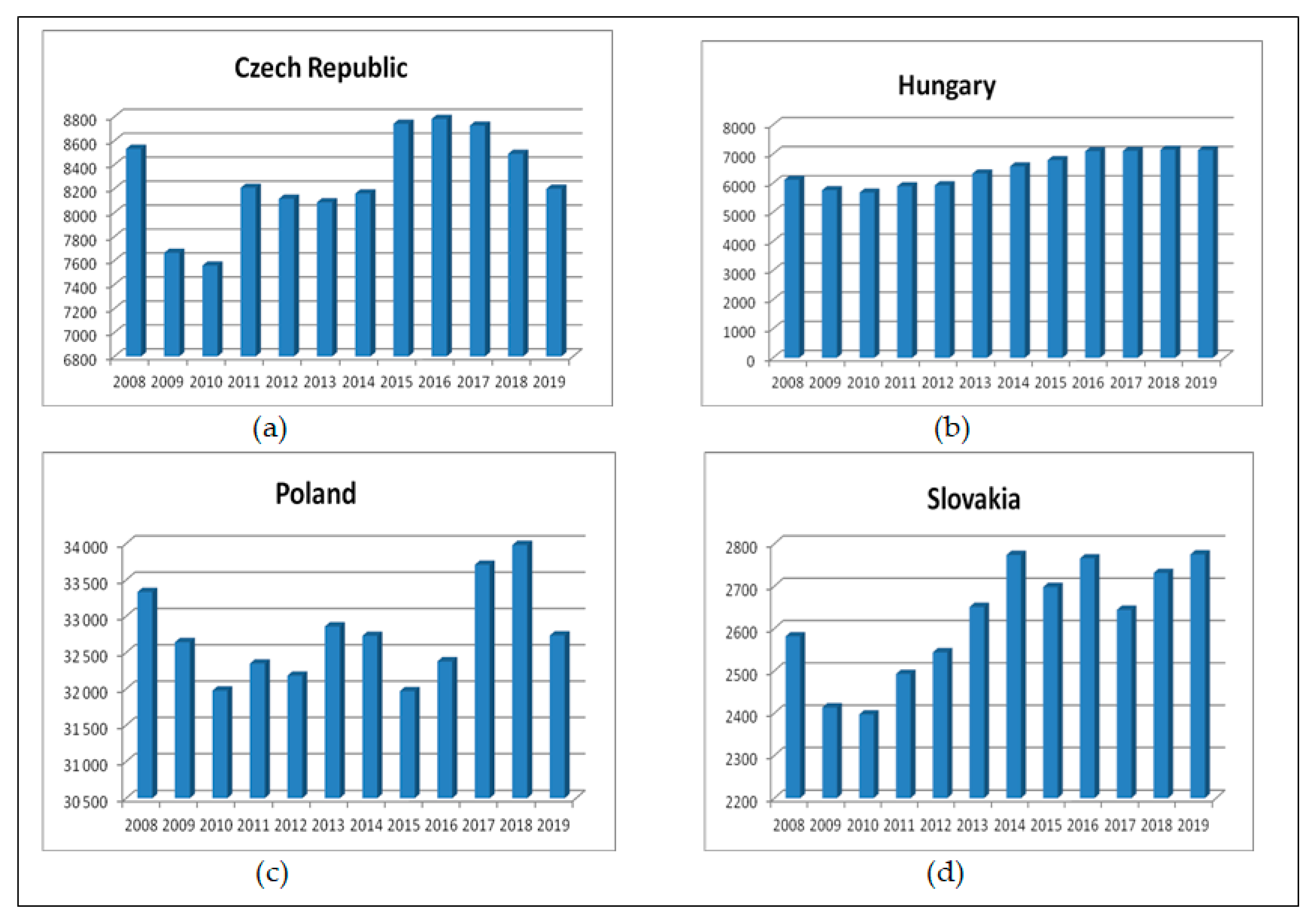
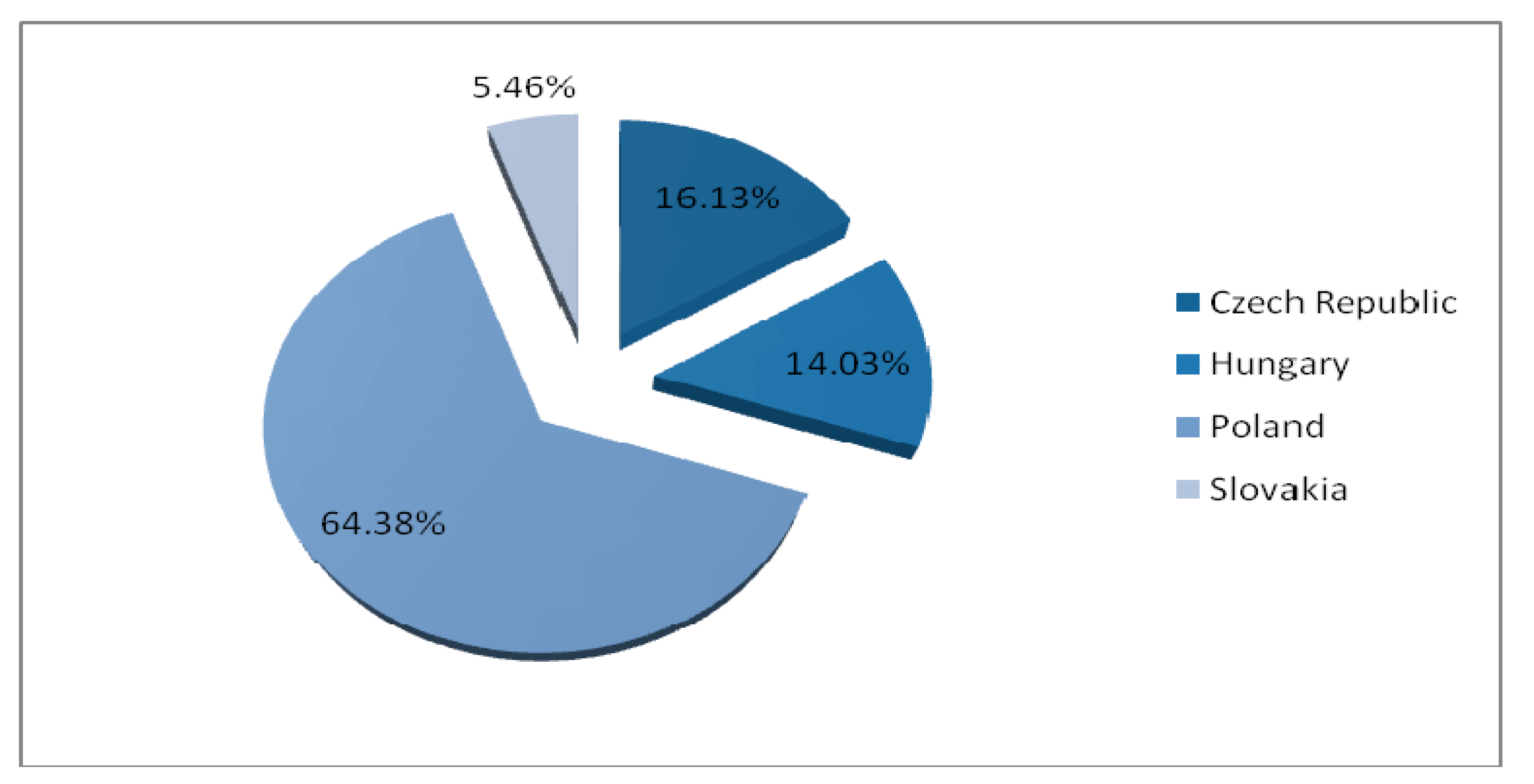
Country	2008	2009	2010	2011	2012	2013	2014	2015	2016	2017	2018	2019	Change in % 2008–2019 *
Czech Republic	8531.51	7663.92	7557.92	8206.84	8115	8086.37	8159.29	8741.21	8781.53	8726.13	8490.15	8198.66	−3.90
Hungary	6113.16	5754.63	5674.03	5889.63	5925.22	6326.21	6572.25	6787.64	7095.35	7105.93	7146.32	7132.74	16.68
Poland	33,333.92	32,643.06	31,975.85	32,349.16	32,182.27	32,859.06	32,729.38	31,968.97	32,377.84	33,708.94	33,980.3	32,735.41	−1.80
Slovakia	2581.29	2413.34	2396.66	2492.36	2543.44	2650.77	2773.25	2697.69	2765.37	2643.66	2730.83	2774.77	7.50

Source: Data from Eurostat [33], * calculations based on data from Eurostat [33].

, Figure 2).

A graphic illustration of greenhouse gas emissions in agriculture in the Visegrad Group countries in 2008–2019 is shown in Figure 2.

It is also worth noting that the share of the agricultural sector in greenhouse gas emissions in Poland, including other countries of the Visegrad Group, amounted to over 64% in 2019. Slovakia had the lowest share of this sector of the economy in greenhouse gas emissions in the studied group (5.46%), Figure 3. As previously stated, this was largely due to the scale of the analyzed economies, but also the differences in the degree of their “greening”. Source emissions data are absolute values, without per capita conversion. This corresponds in our article with the conjunction of the explanatory variables.

As for the variable of the gross value added in agriculture (

Table 2. Gross value added in agriculture, forestry and fishing in 2008–2019/Current prices, million euro/.

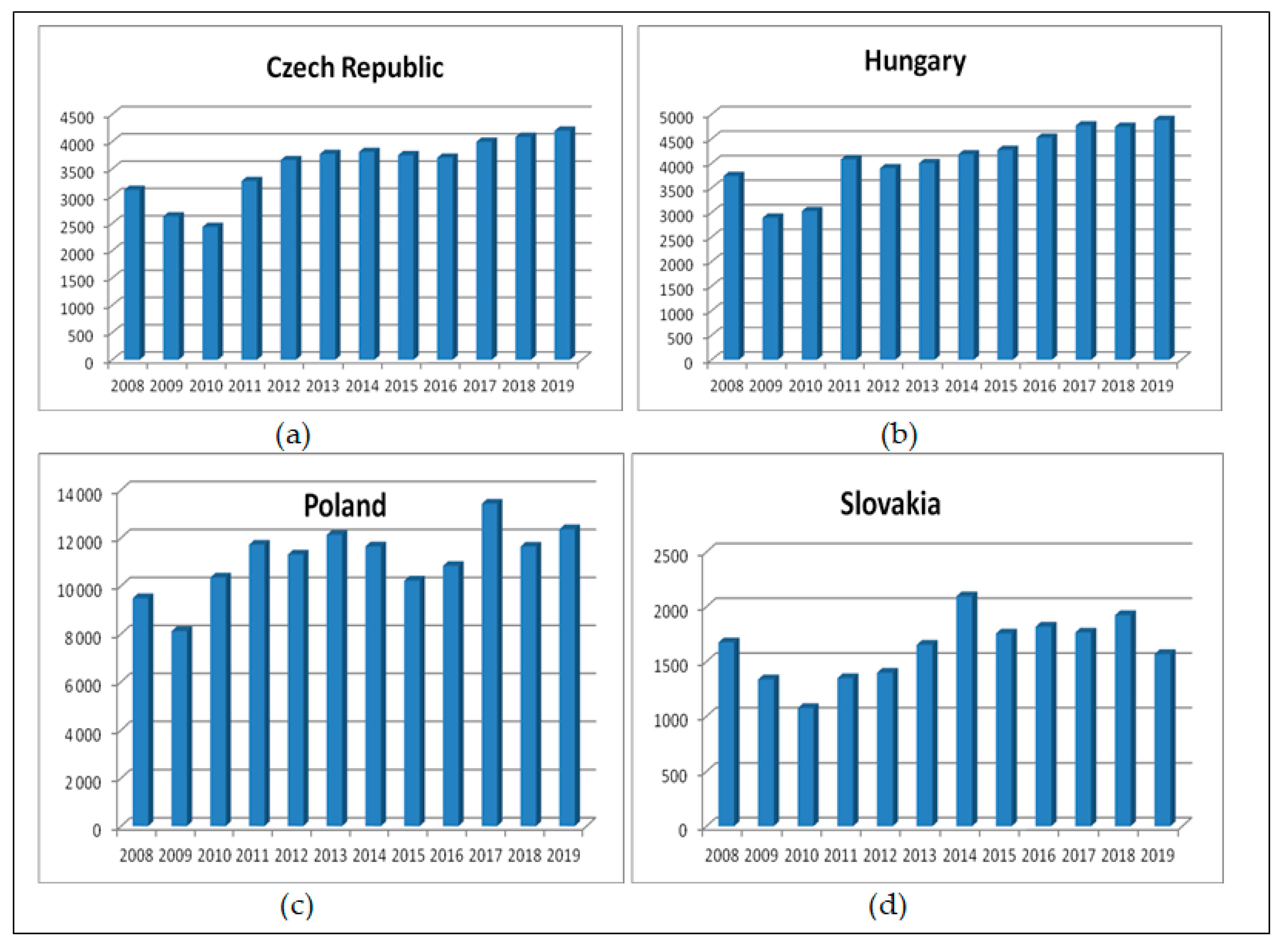
Country	2008	2009	2010	2011	2012	2013	2014	2015	2016	2017	2018	2019	Change in % 2008–2019 *
Czech Republic	3111.5	2627.9	2432.9	3275.2	3660.1	3770.9	3808.9	3749.3	3703.2	3994.5	4084.9	4198.3	34.93
Hungary	3741.1	2891.6	3027.2	4081.2	3900.7	4004.8	4182.6	4274.3	4522.5	4768.8	4743.4	4883.8	30.54
Poland	9490.0	8112.8	10,350.5	11,718.9	11,306.2	12,127.0	11,648.1	10,222.0	10,836.3	13,425.9	11,641.7	12,362.0	30.26
Slovakia	1674.4	1336.5	1075.2	1347.4	1397.6	1652.5	2095.1	1755.9	1818.4	1765.4	1922.6	1568.2	−6.34

Source: Data from [33], * calculations based on data from Eurostat [33].

and Figure 4), it is worth noting that in 2019 Poland ranked first in terms of gross domestic value generated in agriculture among the Visegrad Group countries. It produced EUR 12,362.0 million. Hungary came second with a value of EUR 4884 million, followed by the Czech Republic with a value of EUR 4198.3 million, lower by than Hungary EUR 685.5 million. Slovakia took fourth place, the only one in the group; the gross value generated in the agricultural sector amounted to EUR 1568.2 million and was lower by 6.34% in 2019 than in 2008. Note that the gross value added generated in Polish agriculture in 2019 was about eight times higher than in Slovakia (compare Table 2).

The next part of the article presents the analysis of gross value added in the production sectors of the economy (except agriculture) in the countries of the Visegrad Group, which we treat as a cumulative profitability indicator, estimating economic development (

Table 3. Gross value added in sector of the economy (outside agriculture) in 2008–2019/Current prices, million euro/.

Country	2008	2009	2010	2011	2012	2013	2014	2015	2016	2017	2018	2019	Change in % 2008–2019
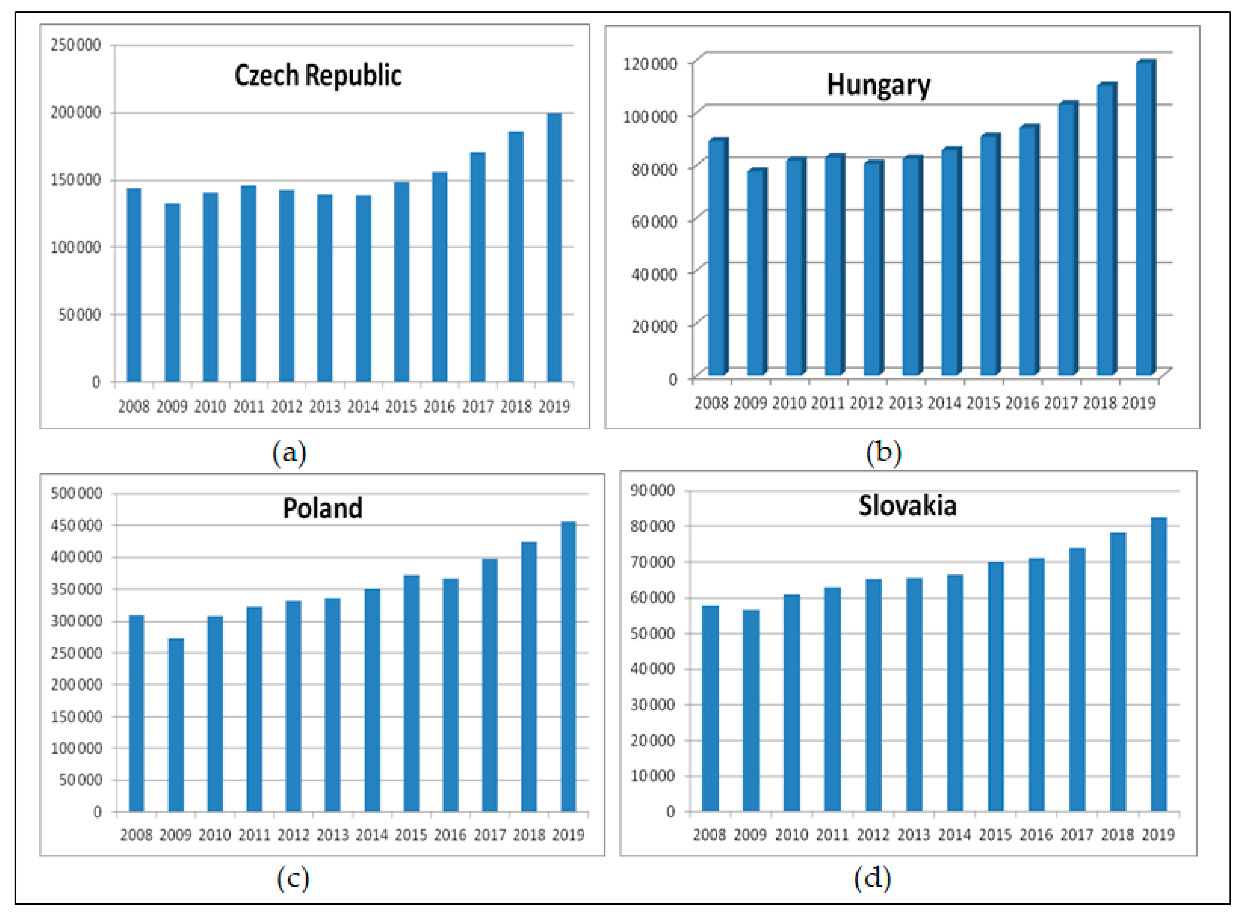
Czech Republic	143,924.7	132,725.2	140,484.7	145,927.9	142,568.9	139,147.3	138,934.3	148,938.6	155,900.2	170,457.4	185,996.6	199,609.2	38.7
Hungary	89,116.3	77,575.1	81,713.6	82,888.6	80,521.5	82,372.8	85,640.3	90,789.8	94,121.7	102,982.4	110,179.9	118,787.3	33.3
Poland	309,849.7	273,300.0	308,327.2	322,066.0	332,248.7	335,876.8	350,773.3	371,706.7	366,475.5	397,080.3	424,233.5	456,751.9	47.4
Slovakia	57,892.9	56,657.0	60,983.3	63,003.6	65,254.5	65,474.7	66,584.9	70,150.9	71,166.4	73,869.5	78,150.1	82,478.7	42.5

Source: Calculations based on data from Eurostat [33].

, Figure 5).

In the years 2008–2019 in Poland, in the group of entities operating in the production sectors of the economy (except agriculture), gross value added increased from EUR 309,849.7 million to EUR 456,751.9 million, i.e., by EUR 146,902.2 million. It was the largest among the surveyed countries, and the smallest in Slovakia. In 2019, a significant diversification of the gross value added in the countries of the Visegrad Group can be noticed, from EUR 82,478.7 million in Slovakia to EUR 456,751.9 million in Poland.

In turn,

Table 4. Effectiveness of greenhouse gas emissions in agriculture in the Visegrad Group countries in 2008–2019.

Country	2008	2009	2010	2011	2012	2013	2014	2015	2016	2017	2018	2019
Czech Republic	2.74	2.92	3.11	3.12	2.22	2.14	2.14	2.33	2.37	2.20	2.08	1.95
Hungary	1.63	1.99	1.87	2.04	1.52	1.58	1.57	1.59	1.57	1.50	1.51	1.46
Poland	3.51	4.02	3.09	3.99	2.85	2.71	2.81	3.13	2.99	2.50	2.92	2.65
Slovakia	1.54	1.81	2.23	1.86	1.82	1.60	1.32	1.54	1.52	1.50	1.42	1.77

Source: Calculations based on data from Eurostat [33].

shows the efficiency of greenhouse gas emissions in agriculture in the Visegrad Group countries in relation to the gross added value produced. In this case, the greenhouse gas emission index per gross value added in agriculture shows the amount of pollutants (here their value) per unit of gross added production. The lower the index, the higher the efficiency of the emission (Table 4).

In 2019, among the countries of the Visegrad Group, Hungary was the country with the least polluted gross value added, followed by Slovakia, followed by the Czech Republic. These countries were characterized by the relatively lowest greenhouse gas emission rate per unit of gross added production, i.e., the highest efficiency of greenhouse gas emissions, as for each EUR 1 million of gross added value generated in agriculture, in 2019 they emitted 1.46–1.95 thousand tons of carbon dioxide equivalent. On the other hand, Poland broadcasted in 2019 2.65 thousand tons of carbon dioxide equivalent. Among the countries of the Visegrad Group, it was the highest pollution indicator for a unit of gross added product (income). It is worth noting here that agriculture is one of the major emitters of greenhouse gases (GHG) and has great potential to mitigate negative climate change [10]. It is worth adding here that, according to the studies by Augustowski, Kułyk, and Michałowska [34], in Poland we deal with various development paths resulting from the diversified allocation of resources in agriculture, particularly including land resources and disproportions in changes in long-term production structures in agriculture, with which organic farming plays an important role in mitigating the effects of greenhouse gas emissions.

4. Results

We repeat, the aim of the study is to identify the correlation between the amount of greenhouse gas emissions, added value from agriculture and economic growth in the Visegrad Group countries measured by the level of gross value added from production in selected sectors, except agriculture and services [33]. Four countries of Central Europe, i.e., the so-called Visegrad Group: Czech Republic, Hungary, Poland and Slovakia was studied 2008–2019. This group of countries was selected due to the representation of Central and Eastern Europe in the EU, their political integration and subordination to the Common Agricultural Policy. The article searched for an answer to the following question: Was the world economic crisis of 2008–2009 marked by changes in the amount of greenhouse gas emissions in agriculture in the analyzed group of countries? and did their recovery from the global crisis of 2008–2009 have an impact on gas emissions in their agriculture in a later period? The question was also asked whether the differences in the amount of greenhouse gas emissions in individual countries are deepening or, on the contrary, they are being reduced? It should also be asked whether the research results allow us to believe that the global economic crisis may be treated as a kind of warning for a negative increase in the “carbon footprint” in agriculture in the surveyed countries, or vice versa? Due to the objectives of the article, it was decided to use the panel model, which allows for a broader and more precise analysis of the relationships in the studied countries. The time range covers the years 2008–2019, i.e., two economic periods: 2008–2014, when there was a downward trend in the general profitability index in the productive sectors of the economy studied here, including agriculture, and 2015–2019, when an upward trend in the general index was noted profitability in the productive sectors of the economy, including agriculture. The study used regression analysis using a panel model with fixed effects to analyze the correlation between the amount of greenhouse gas emissions and selected determinants in relation to agriculture. In the procedure, the determined individual effects are eliminated by averaging the model with respect to years (index t). The dependent variable was the amount of greenhouse gas emissions (GHG), while the gross value addend from agriculture (gross value addend, VA) and the gross value added of goods and services produced in the economy outside agriculture (gross value addend, GVA) are independent variables. The data used in the model were log transformed. The time series had the full range of data for 2008–2019. In the research process, relationships between the variables were searched for, i.e., the answers to whether a given variable influences others and how. In the further part of the research process, the analyzed period was divided into two sub-periods in order to determine the relationships between the variables illustrating the added value (here, economic growth, also in agriculture in the years of different economic prosperity) and the amount of greenhouse gas emissions. The 2008–2014 and 2015–2019 sub-periods were adopted, assuming that the former also covers the period of the global crisis of 2008–2009, and that the latter has been gradually overcome. The data used in the study were obtained from the resources of Eurostat [33].

Table 5. Descriptive statistics for the adopted parameters in the studied countries of the Visegrad Group in 2008–2019.

Variable		Mean	Std. Dev.	Min	Max	Observations
GHG	overall	3.914694	0.3980537	3.379606	4.531227	N = 48
	between		0.4539479	3.418077	4.514962	n = 4
	within		0.0246346	3.859963	3.960153	T = 12
VA	overall	3.598198	0.309883	3.031489	4.127943	N = 48
	between		0.3449395	3.202155	4.042006	n = 4
	within		0.0699381	3.427531	3.717247	T = 12
GVA	overall	5.128227	0.280481	4.753254	5.65968	N = 48
	between		0.3142467	4.827547	5.544819	n = 4
	within		0.0550506	5.020048	5.245814	T = 12

Legend: GHG—Greenhouse gases (including CO₂, N₂O in CO₂ equivalent, CH₄ in CO₂ equivalent, HFC in CO₂ equivalent, PFC in CO₂ equivalent, SF6 in CO₂ equivalent, NF3 in CO₂ equivalent); VA—gross value addend in agriculture, forestry and fishing in the Visegrad Group; GVA—gross value added in the production sectors of the economy (except agriculture, including industry, construction, trade, transport, communications and other service activities). The data used in the model were log transformed. Source: Calculations based on data from Eurostat [33], generated using the program STATA.

presents descriptive statistics for the adopted parameters in the analyzed countries in 2008–2019, and in the following tables the model is estimated taking into account the presence of fixed effects (FE) for individual countries (

Table 6. Fixed effects models for the countries of the Visegrad Group.

Fixed-effects (within) regression				Number of obs =		48
Group variable: Country				Number of group =		4
R-squared:				Obs per group:
	within =	0.5726			min =	12
	between =	0.9972			avg =	12.0
	overall =	0.9709			max =	12
				F (2, 42) =		28.14
Corr(u_i,Xb) = 0.9768				Prob > F =		0.0000
GHG	Coefficient	Std. err.	t	P > |t|	[95% conf. interval]
VA	0.2039179	0.0465662	4.38	0.000	0.1099436	0.2978923
GVA	0.1074956	0.0591593	1.82	0.076	−0.0118927	0.2268839
_cons	2.629695	0.2332494	11.27	0.000	2.158979	3.100411
sigma_u	0.35182242
sigma_e	0.01703577
rho	0.99766084
F test that all u_i = 0: F (3, 42) = 197.47					Prob > F = 0.0000

The data used in the model were log transformed. Source: Calculations based on data from Eurostat [33], generated using the program STATA.

) and years (

Table 7. Regression model for the countries of the Visegrad Group.

GHG	Coefficient	Std. Err.	t	P > |t|	[95% Conf. Interval]
VA	0.2039179	0.0465662	4.38	0.000	0.1099436	0.2978923
GVA	0.1074956	0.0591593	1.82	0.076	−0.0118927	0.2268839
Country
Hungary	−0.0970543	0.0169385	−5.73	0.000	−0.1312375	−0.062871
Poland	0.4571834	0.0200857	22.76	0.000	0.4166487	0.497718
Slovakia	−0.3913366	0.0176467	−22.18	0.000	−0.426949	−0.3557242
_cons	2.637497	0.2363717	11.16	0.000	2.160479	3.114514

The data used in the model were log transformed. Source: Calculations based on data from Eurostat [33], generated using the program STATA.

).

The Greenhouse gases (GHG) variable consists of 48 observations (4 countries*12), the estimated mean (overall) is 3.91, the standard deviation is 0.39, and the standard deviation between the countries studied is 0.45 on average, and within the Visegrad Group countries it is 0.024 in the period 2008–2019, i.e., 12 years. The variability over time turned out to be lower than the variability in space over a period of one year. The situation is similar in the case of gross value added from agriculture (VA) and gross value added (GVA) for sectors of the economy outside agriculture; the variability with time is less than in space. The data contained in the table show that the annual dynamics have less impact on the variability of the explained characteristics than the variability between individual units in a given year.

In the first step, the model was estimated taking into account the fixed effects (FE) for the studied countries (Table 6). The study also considered a panel model with variable effects. For testing random effects, the Breusch–Pagan test [32] was used, based on Lagrange multipliers, which did not confirm the choice of the random term decomposition model for this test, as evidenced by the low value of the test statistic (0.43) with a p value of 0.2557. On the other hand, the choice between the estimator of fixed effects and the estimator of random individual effects for individual countries of the Visegrad Group was made on the basis of the Hausman test [31]. For the Hausman test, we have H = 41.63 with a p value of 0.0000, the test statistics justified the choice of a panel model with constant effects for the studied group of countries.

As the model shows, the correlation coefficient between the fixed effects for the country and the variable x matrix is high (corr (u_i, Xb) and amounts to 0.9768. Independent variables: gross value added from agriculture (VA) and gross value added (GVA) in the production sectors of the economy (apart from agriculture) affect the growing amount of greenhouse gas emissions. We also looked for answers to whether the differences in the amount of greenhouse gas emissions deepen in individual countries or, on the contrary? There is a reduction (Czech Republic as a base variable), Hungary and Slovakia favor the reduction of greenhouse gas emissions, and for Poland, an increase (Table 7).

In the next step, the model was estimated taking into account the fixed effects (FE) for individual years (

Table 8. Fixed effects models covering the years 2008–2019.

Fixed-effects (within) regression				Number of obs =		48
Group variable: Country				Number of groups =		4
R-squared:				Obs per group:
	within =	0.6844			min =	12
	between =	0.4998			avg =	12.0
	overall =	0.2693			max =	12
				F(13, 31) =		5.17
Corr(u_i,Xb) = 0.4652				Prob > F =		0.0001
GHG	Coefficient	Std. err.	t	P > |t|	[95% conf. interval]
VA	0.1367941	0.0758759	1.80	0.081	−0.0179559	0.291544
GVA	−0.1012542	0.1872679	−0.54	0.593	−0.4831897	0.2806813
YEAR
2009	−0.0198059	0.0158885	−1.25	0.222	−0.522107	0.0125989
2010	−0.0224365	0.013896	−1.61	0.117	−0.0507775	0.0059045
2011	−0.165687	0.0121779	−1.36	0.183	−0.0414057	0.0082683
2012	−0.0163311	0.0122799	−1.33	0.193	−0.0413762	0.008714
2013	−0.0070815	0.0128911	−0.55	0.587	−0.033373	0.01921
2014	−0.001371	0.0141708	−0.01	0.992	−0.0290386	0.0287645
2015	0.0123848	0.0154394	0.80	0.429	−0.019104	0.0438736
2016	0.0206279	0.0167982	1.23	0.229	−0.0136322	0.054888
2017	0.0181967	0.0220249	0.83	0.415	−0.267233	0.0631167
2018	0.0238741	0.0264912	0.90	0.374	−0.030155	0.779031
2019	0.0218579	0.0311601	0.70	0.488	−0.0416935	0.0854093
_cons	3.940522	1.009824	3.90	0.000	1.880972	6.000071
sigma_u	0.43885062
sigma_e	0.1704015
rho	0.99849457	(fraction of variance due to u_i)
F test that all u_i = 0: F(3, 31) = 25.23					Prob > F = 0.0000

The data used in the model were log transformed. Source: Calculations based on data from Eurostat [33], generated using the program STATA.

) in order to confirm or reject the hypothesis made in the introduction that the economic crisis of 2008–2009 had a positive impact on the amount of greenhouse gas emissions in the following years 2009–2019, and that overcoming the crisis also had a positive impact on greenhouse gas emissions in agriculture in the surveyed countries and can be treated as a premise for a strategy for the further development of agriculture in a more sustainable way. The results are as in Table 8. They show that in the years 2009–2014, compared to 2008, a reduction in greenhouse gas emissions can be observed, while in 2015–2019 they increased.

In the next step, it was considered whether the introduction of time variables for the entire group was statistically significant. The following values were obtained:

(1) 2009.YEAR = 0 (2) 2010.YEAR = 0 (3) 2011.YEAR = 0 (4) 2021.YEAR = 0 (5) 2013.YEAR = 0 (6) 2014.YEAR = 0	(7) 2015.YEAR = 0 (8) 2016.YEAR = 0 (9) 2017.YEAR = 0 (10) 2018.YEAR = 0 (11) 2019.YEAR = 0
F(11, 31) = 1.00  Prob > F = 0.4699

The value of Prob > F-value is low and amounts to 0.4699, which means that there is no statistically significant evidence to reject the null hypothesis that it was important to include the fixed effects (FE) for individual years in the model. As can be seen in this model, taking into account the fixed effects (FE) for subsequent years, the variable value added from agriculture (VA) increased the amount of greenhouse gas emissions, and the gross value added (GVA) of the examined non-agricultural sectors led to a reduction in the amount of greenhouse gas emissions.

The data in Table 8 showing the model estimation carried out, taking into account the fixed effects (FE) for subsequent years, show that in the period 2009–2014 (2008 was assumed as the base) there was a reduction in greenhouse gas emissions, and in 2015–2019 there was an increase. The years 2008–2019, due to the global economic crisis (2008–2009) and the subsequent successive recovery from the economic slowdown, were difficult for the agricultural sector and the entire economy, which reflects the deterioration of the economic situation of the production sectors of the economy in the analyzed countries, also outside agriculture. In this part of the study, research was carried out for the two periods distinguished 2008–2014 (

Table 9. Fixed-effects models for the countries of the Visegrad Group in 2008–2014.

Fixed-effects (within) regression				Number of obs =		28
Group variable: Country				Number of group =		4
R-squared:				Obs per group:
	within =	0.4928			min =	7
	between =	0.9914			avg =	7.0
	overall =	0.9663			max =	7
				F(2, 22) =		10.69
Corr(u_i,Xb) = 0.9765				Prob > F =		0.0006
GHG	Coefficient	Std. err.	t	P > |t|	[95% conf. interval]
VA	0.1629763	0.0444603	3.67	0.001	0.0707713	0.2551814
GVA	0.0567004	0.1330423	0.43	0.674	−0.2192125	0.3326132
_cons	3.031348	0.6075967	4.99	0.000	1.771269	4.291426
sigma_u	0.38620103
sigma_e	0.0138818
rho	0.99870966	(fraction of variance due to u_i)
F test that all u_i = 0: F(3, 22) = 96.34					Prob > F = 0.0000

The data used in the model were log transformed. Source: Calculations based on data from Eurostat [33], generated using the program STATA.

) and 2015–2019 (

Table 10. Fixed-effects models for the countries of the Visegrad Group in 2015–2019.

Fixed-effects (within) regression				Number of obs =		20
Group variable: Country				Number of groups =		4
R-squared:				Obs per group:
	within =	0.0378			min =	5
	between =	0.8909			avg =	5.0
	overall =	0.8791			max =	5
				F(2, 14) =		0.27
Corr(u_i,Xb) = 0.9327				Prob > F =		0.7636
GHG	Coefficient	Std. err.	t	P > |t|	[95% conf. interval]
VA	0.721283	0.0978144	0.74	0.473	−0.1376628	0.2819193
GVA	−0.0223824	0.073923	−0.30	0.767	−0.1809316	0.1361667
_cons	3.786861	0.369626	10.25	0.000	2.994092	4.57963
sigma_u	0.42927612
sigma_e	0.01109741
rho	0.99933215	(fraction of variance due to u_i)
F test that all u_i = 0: F(3, 14) = 82.53					Prob > F = 0.0000

The data used in the model were log transformed. Source: Calculations based on data from Eurostat [33], generated using the program STATA.

) in order to answer whether the global economic crisis of 2008–2009 was marked by progressive changes (increases?) in greenhouse gas emissions in the analyzed agriculture groups of countries and whether the subsequent recovery from the crisis had an impact on the emission of gases in their agriculture.

As results from the model presented above for individual countries of the Visegrad Group in 2008–2014, the correlation coefficient between the fixed effects for a given country and the matrix of variable x was high (corr (u_i, Xb) and amounted to 0.9765, which means the suggestion that the variables added value from agriculture (VA) and gross value added from the analyzed non-agricultural industries (GVA) increased the amount of greenhouse gas emissions in a given period.

Fixed-effects models for the countries of the Visegrad Group in 2015–2019 are shown in the Table 10.

On the other hand, from the model developed for the Visegrad Group countries in 2015-2019, the correlation coefficient between the fixed effects for individual countries and the variable × matrix is also high (corr (u_i, Xb) and amounts to 0.9327 from agriculture (VA) increases in the amount of greenhouse gas emissions, while the gross value added (GVA) for non-agricultural industries reduces it. In general, it can be assumed that the recovery from the crisis also had a positive impact on the emission of greenhouse gases in the production sectors of the analyzed countries and can be treated as a premise for to the development of agriculture as part of a strategy limiting the negative effects of industrial development, i.e., more sustainability.

5. Discussion

The results of the research by Zaharia and Antonescu [4] show the existence of a correlation between agriculture and climate change and underline the importance of good GHG emissions management from agriculture for the future of the natural environment. In the light of the results of our research, it can be noticed that the factors influencing the changes in greenhouse gas emissions in the Visegrad Group countries in 2009–2014 were the increased emissivity and economic recovery after the global economic crisis, resulting from the upward trend in the profitability index in the production sectors of the economy and also in agriculture.

The research results also correlate with the research of Perrier, Guivarch and Boucher [9], who indicate that greenhouse gas emissions were mostly due to the reduction in the intensity of carbon dioxide emissions, largely compensated by economic recovery. Changes in the production system, mainly due to the increase in imports, also played an important role in the decline in emissions, evolution of end-demand patterns and declining emissions from heating households and private transport, with little compensation for population growth [9]. Researchers Perrier, Guivarch and Boucher [9] also concluded that the most important drivers of changes in greenhouse gas emissions in the EU in 2009–2014 were increased emissions and economic recovery, as this study confirms. Florea, Bădîrcea, Pîrvu, Manta, Doran, and Jianu [35] studied the impact of agriculture and renewable energy on climate change in the countries of Central and Eastern Europe (11 countries of Central and Eastern Europe (CEEC)) in the years 2000–2017. These studies led to the estimation of the long-term relationship between the variables. They also used the Granger causality test based on the ARDL—Error Correction Model (ECM) and Pairwise Granger. The results obtained revealed, in the long term, two two-way relationships between agriculture and economic growth, and two one-way relationships between agriculture and greenhouse gas emissions and renewable energy. In the light of the results obtained from the studies presented above, one can also notice a large differentiation in terms of the determinants of greenhouse gas emissions in the studied countries. Balogh [36] came to similar conclusions, showing that the so-called carbon footprint was strongly associated with earlier economic development and tended to decline when a turning point was reached. This area of research was also the subject of this analysis, which confirmed the correctness of this conclusion. Similar observations result from the literature review of the research methods adopted by the authors Florea, Bădîrcea, Pîrvu, Manta, Doran, and Jianu [35].

The conducted research, as well as the studies of other authors Liobikienė, Butkus [6], González-Sánchez, and Martín-Ortega [7] prove that the applied panel model with constant effects is useful for analyzing the dependencies occurring in the studied countries. Research using regression models (using first difference estimation (FD), fixed effects (FE) and random effects (RE)) based on panel data was used by Liobikienė and Butkus [6] to find out how the primary energy consumption, the share of renewable energy sources and economic growth affect changes in greenhouse gas emissions in the EU-28 countries [6]. González-Sánchez and Martín-Ortega [7] identified the main determinants that influence the increase in greenhouse gas emissions and assessed their impact and differences between countries in Europe. They used two models for empirical research: a linear panel data model and a multiple linear regression model for each country. The first model was used to assess whether the selected determinants are relevant to explain the increase in GHG emissions in the EU. The second model was used to evaluate the differences in the effect of each determinant. Researchers concluded that the uneven impact of the main determinants of the increase in GHG emissions suggests that the differentiated application of European policies at the national level will increase the effectiveness of mitigation measures in Europe [7]. On the other hand, Rokicki, Koszela, Ochnio, Golonko, Zak, E.K. Szczepaniuk, H. Szczepaniuk, Perkowska [10] noted in empirical studies that greenhouse gas emissions were highly concentrated in several EU countries with the most developed agriculture. In the years 2004–2017, there were no changes in the level of emission concentration there. Nevertheless, it can be assumed that the level of greenhouse gases from agriculture depended on the current situation of agriculture in the economy of a given country.

6. Conclusions

The question of the impact of agriculture on greenhouse gas emissions is complex and multi-faceted. The study identifies the correlation between the amount of greenhouse gas emissions, added value from agriculture and economic growth in the Visegrad Group countries using panel models. The presented fixed-effects model for the Visegrad Group countries allowed us to indicate that greenhouse gas emissions are positively correlated with the added value from agriculture and economic growth in the Visegrad Group countries. The increase in the level of these variables had a positive effect on the amount of greenhouse gas emissions in the countries of the Visegrad Group. In the research process, the method used was verified with the Hausman test, which helped to answer the question which of the effects (constant or random) occur in the analyzed group of countries. The Breusch–Pagan test also did not confirm the validity of using the model with random component decomposition. The obtained results showed the advantage of panel models with fixed effects over panel models with variable effects for the studied countries of the Visegrad Group.

Taking into account the efficiency of greenhouse gas emissions in agriculture in the Visegrad Group countries, in relation to the gross value added that was produced, the country with the least polluted gross value added was Hungary, followed by Slovakia, followed by the Czech Republic. These countries were characterized by the relatively lowest GHG emission rate per unit of gross added production, i.e., the highest GHG emission efficiency, in contrast to Poland with the relatively highest GHG emission rate. However, the research presented in the study made it possible to verify the research hypotheses positively adopted at the outset; the first, significant correlation exists between the volume of greenhouse gas emissions and economic growth in the countries of the Visegrad Group. The factors that had the greatest impact on changes in greenhouse gas emissions in the Visegrad Group countries in 2009–2014 were: increased emissions and economic recovery after the global economic crisis, confirmed by an upward trend in the profitability index in production sectors of the economy, including agriculture. The results of the research suggest also that the recovery from the crisis had a statistically positive (i.e., increasing) effect on greenhouse gas emissions in the production sectors of the economy, including agriculture in the researched countries, and may be treated as a premise for a strategy for the development of agriculture limiting the negative effects of its industrial development for more sustainable development. The conducted empirical studies also provide grounds for concluding that the identification of determinants influencing the increase in greenhouse gas emissions and the assessment of their impact, as well as the differences between the countries in the Visegrad Group, are positive premises for supporting economic policy in the implementation of programs aimed at counteracting greenhouse gas emissions. In the opinion of the authors, the article may also turn out to be useful for decision makers of economic policy, showing the premises for its implementation, setting goals, as well as changes in the scope of actions taken, in connection with the need to stop negative climate changes resulting from global warming.

References

- Lynch, J.; Cain, M.; Frame, D.; Pierrehumbert, R. Agriculture’s Contribution to Climate Change and Role in Mitigation Is Distinct from Predominantly Fossil CO2-Emitting Sectors. Front. Sustain. Food Syst. 2021, 4, 518039. [Google Scholar] [CrossRef] [PubMed]
- EEA. EEA Greenhouse Gases—Data Viewer. Available online: https://www.eea.europa.eu/data-and-maps/data/data-viewers/greenhouse-gases-viewer/ (accessed on 4 January 2022).
- Report Intergovernmental Panel on Climate Change (IPCC). Climate Change Widespread, Rapid, and Intensifying. 2021. Available online: https://www.ipcc.ch/2021/08/09/ar6-wg1-20210809-pr/data (accessed on 20 January 2022).
- Zaharia, A.; Antonescu, A.-G. Agriculture, Greenhouse Gas Emissions and CLIMATE Change. In Proceedings of the 14th International Multidisciplinary Scientific Geoconference (SGEM 2014), Albena, Bulgaria, 17–26 June 2014; pp. 17–24. [Google Scholar]
- Mairura, S.F.; Musafiri, C.M.; Kiboi, M.N.; Macharia, J.M.; Ng’etich, O.; Shisanya, C.A.; Okeyo, J.M.; Mugendi, D.N.; Okwuosa, E.A.; Ngetich, F.K. Determinants of farmers’ perceptions of climate variability, mitigation, and adaptation strategies in the central highlands of Kenya. Weather. Clim. Extrem. 2021, 34, 100374. [Google Scholar] [CrossRef]
- Liobikienė, G.; Butkus, M. Determinants of greenhouse gas emissions: A new multiplicative approach analysing the impact of energy efficiency, renewable energy, and sector mix. J. Clean. Prod. 2021, 309, 127233. [Google Scholar] [CrossRef]
- González-Sánchez, M.; Martín-Ortega, J.L. Greenhouse Gas Emissions Growth in Europe: A Comparative Analysis of Determinants. Sustainability 2020, 12, 1012. [Google Scholar] [CrossRef] [Green Version]
- Su, M.; Pauleit, S.; Yin, X.; Zheng, Y.; Chen, S.; Xu, C. Greenhouse gas emission accounting for EU member states from 1991 to 2012. Appl. Energy 2016, 184, 759–768. [Google Scholar] [CrossRef]
- Perrier, Q.; Guivarch, C.; Boucher, O. Diversity of greenhouse gas emission drivers across European countries since the 2008 crisis. Clim. Policy 2019, 19, 1067–1087. [Google Scholar] [CrossRef]
- Rokicki, T.; Koszela, G.; Ochnio, L.; Golonko, M.; Zak, A.; Szczepaniuk, E.K.; Szczepaniuk, H.; Perkowska, A. Greenhouse Gas Emissions by Agriculture in EU Countries. 2020. Available online: https://ros.edu.pl/images/roczniki/2020/057_ROS_V22_R2020.pdf (accessed on 2 January 2022).
- Özçağ, M.; Yilmaz, B.; Sofuoğlu, E. Türkiye’de Sanayi ve Tarım Sektörlerinde Seragazı Emisyonlarının Belirleyicileri: İndeks Ayrıştırma Analizi. Uluslararası İlişkiler Derg. 2017, 14, 175–195. [Google Scholar] [CrossRef]
- Ivanovski, K.; Churchill, S.A. Convergence and determinants of greenhouse gas emissions in Australia: A regional analysis. Energy Econ. 2020, 92, 104971. [Google Scholar] [CrossRef]
- Benbi, D. Carbon footprint and agricultural sustainability nexus in an intensively cultivated region of Indo-Gangetic Plains. Sci. Total Environ. 2018, 644, 611–623. [Google Scholar] [CrossRef]
- Jovanović, M.; Kascelan, L.; Despotović, A.; Kašćelan, V. The Impact of Agro-Economic Factors on GHG Emissions: Evidence from European Developing and Advanced Economies. Sustainability 2015, 7, 16290–16310. [Google Scholar] [CrossRef] [Green Version]
- Constantin, M.; Rădulescu, I.D.; Andrei, J.V.; Chivu, L.; Erokhin, V.; Gao, T. A perspective on agricultural labor productivity and greenhouse gas emissions in context of the Common Agricultural Policy exigencies. Ekon. Poljopr. 2021, 68, 53–67. [Google Scholar] [CrossRef]
- Prandecki, K.; Gajos, E. The Share of Agriculture in Greenhouse Gas Emissions in European Union Countries–Valuation. In Proceedings of the 8th International Scientific Conference Rural Development 2017: Bioeconomy Challenges, Kaunas, Lithuania, 23-24 November 2017; pp. 1267–1272. [Google Scholar] [CrossRef] [Green Version]
- McGinn, S.M. Measuring greenhouse gas emissions from point sources in agriculture. Can. J. Soil Sci. 2006, 86, 355–371. [Google Scholar] [CrossRef]
- Mrówczyńska-Kamińska, A.; Bajan, B.; Pawłowski, K.P.; Genstwa, N.; Zmyślona, J. Greenhouse gas emissions intensity of food production systems and its determinants. PLoS ONE 2021, 16, 0250995. [Google Scholar] [CrossRef] [PubMed]
- Israel, M.A.; Amikuzuno, J.; Danso-Abbeam, G. Assessing farmers’ contribution to greenhouse gas emission and the impact of adopting climate-smart agriculture on mitigation. Ecol. Process. 2020, 9, 1–10. [Google Scholar] [CrossRef]
- Wettemann, P.J.C. Productivity Change of Arable Farms with Regard to Greenhouse Gas Emissions. Ger. J. Agric. Econ. 2017, 66, 26–43. [Google Scholar]
- Phiri, J.; Malec, K.; Kapuka, A.; Maitah, M.; Appiah-Kubi, S.N.K.; Gebeltová, Z.; Bowa, M.; Maitah, K. Impact of Agriculture and Energy on CO2 Emissions in Zambia. Energies 2021, 14, 8339. [Google Scholar] [CrossRef]
- Alkan, A.; Binatli, A.O. Is Production or Consumption the Determiner? Sources of Turkey’s CO2 Emissions between 1990–2015 and Policy Implications. Hacet. Üniversitesi İktisadi Ve İdari Bilimler Fakültesi Derg. 2021, 39, 359–378. Available online: https://mpra.ub.uni-muenchen.de/111635/ (accessed on 5 March 2022). [CrossRef]
- Dzikuć, M.; Wyrobek, J.; Popławski, Ł. Economic Determinants of Low-Carbon Development in the Visegrad Group Countries. Energies 2021, 14, 3823. [Google Scholar] [CrossRef]
- Ruzickova, K. The agricultural companies and their value spread within the Visegrad Group. Ann. Agric. Econ. Rural. Dev. 2013, 100, 91–102. [Google Scholar]
- Střeleček, F.; Lososová, J.; Zdeněk, R. Comparison of subsidies in the Visegrad Group after the EU accession. Agric. Econ. 2009, 55, 415–423. [Google Scholar] [CrossRef] [Green Version]
- Tucki, K.; Krzywonos, M.; Orynycz, O.; Kupczyk, A.; Bączyk, A.; Wielewska, I. Analysis of the Possibility of Fulfilling the Paris Agreement by the Visegrad Group Countries. Sustainability 2021, 13, 8826. [Google Scholar] [CrossRef]
- Czyżewski, A.; Grzyb, A.; Matuszczak, A.; Michałowska, M. Factors for Bioeconomy Development in EU Countries with Different Overall Levels of Economic Development. Energies 2021, 14, 3182. [Google Scholar] [CrossRef]
- Kulshreshtha, S.; Junkins, B.; Desjardins, R. Prioritizing greenhouse gas emission mitigation measures for agriculture. Agric. Syst. 2000, 66, 145–166. [Google Scholar] [CrossRef]
- Mielcarek-Bocheńska, P.; Rzeźnik, W. Greenhouse Gas Emissions from Agriculture in EU Countries—State and Perspectives. Atmosphere 2021, 12, 1396. [Google Scholar] [CrossRef]
- Zhang, Z.; Hong, W.-C. Application of variational mode decomposition and chaotic grey wolf optimizer with support vector regression for forecasting electric loads. Knowl. Based Syst. 2021, 228, 107297. [Google Scholar] [CrossRef]
- Hausman, J.A. Specification Tests in Econometrics. Econometrica 1978, 46, 1251–1271. [Google Scholar] [CrossRef] [Green Version]
- Breusch, T.S.; Pagan, A.R. The Lagrange Multiplier Test and its Applications to Model Specification in Econometrics. Rev. Econ. Stud. 1980, 47, 239–253. [Google Scholar] [CrossRef]
- Eurostat. Available online: http://appsso.eurostat.ec.europa.eu/nui/submitViewTableAction.do (accessed on 4 January 2022).
- Augustowski, Ł.; Kułyk, P.; Michałowska, M. Spatial Diversity of The Growth of Organic Farming in Poland, 2020. In Proceedings of the 35th International Business Information Management Association Conference (IBIMA): VISION 2025: Education Excellence and Management of Innovations through Sustainable Economic Competitive Advantage, Madrid, Spain, 1–2 April 2020; International Business Information Management Association (IBIMA): Norristown, PA, USA; pp. 14632–14640. [Google Scholar]
- Florea, N.M.; Badircea, R.M.; Pirvu, R.C.; Manta, A.G.; Doran, M.D.; Jianu, E. The impact of agriculture and renewable energy on climate change in Central and East European Countries. Agric. Econ. 2020, 66, 447–457. [Google Scholar] [CrossRef]
- Balogh, J.M. Agriculture-specific determinants of carbon footprint. Stud. Agric. Econ. 2019, 121, 166–170. [Google Scholar] [CrossRef]