EOSOLAR Project: Assessment of Wind Resources of a Coastal Equatorial Region of Brazil—Overview and Preliminary Results

Abstract

The EOSOLAR project was designed to investigate the structure of the atmospheric boundary layer in an equatorial coastal zone, where the discontinuity of surface conditions induces non-stationarity gradients of wind speeds and the development of internal boundary layers. The proposed methodology considers several aspects of the sea–land transition meteorology that are essential for precisely estimating wind–solar energy potential and assessment of structural loads on wind turbines. Infrared (LIDAR) and acoustic (SODAR) ground-based remote sensing instruments and micrometeorological towers were installed in a near-shore equatorial area of northeast Brazil, in order to provide a comprehensive view of meteorological processes. This paper reports a description of the project study area, methodology, and instrumentation used. Details of instruments configurations, a validation of micrometeorology towers, and a comparison between the LIDAR and SODAR are presented. Results of the first field campaign measuring the coastal flow, integrating the micrometeorological tower and LIDAR observations are described.

1. Introduction

Atmospheric flows in coastal regions play an important role in both the assessment of the potential and the operation of many wind farms in Brazil. Because of the South Atlantic trade winds, which are strong and stable for generation, the Northeast region has the highest concentration of wind farms in Brazil. More than 85% of the installed wind capacity comes from this region [1] with most of them (76%) placed in coastal areas [2]. The assessment of offshore wind in Brazilian waters [3,4,5,6] has already identified a large potential to be explored, opening new perspectives for the exploration of the marine environment. There are currently 80 GW distributed in 36 offshore projects under environmental licensing at the Brazilian Institute of the Environment and Renewable Natural Resources (IBAMA, 2022).

Despite the interest in siting turbines in coastal and offshore areas of northeast Brazil, the understanding of wind characteristics that are relevant to the industry is hindered by the lack of detailed observations of the equatorial margin. Therefore, closing this gap has become a key step for the planning and optimization of future wind farms. Since most onshore and offshore wind turbines are deployed within a few kilometers of the coastline, the EOSOLAR project results should overcome the present lack of information, providing high-quality datasets for resource assessment and model validation.

As the air flows from sea to land, physical processes will change the structure of the atmospheric boundary layer, impacting winds magnitude, vertical shear, and turbulence. The discontinuity caused by abrupt changes of surface roughness and thermal properties promotes the development of the internal boundary layers, leading to significant horizontal gradients of wind speeds [7,8]. By means of a theoretical model of flow over a change in surface roughness, Barthelmie (1999) demonstrated that, for typical values of geostrophic winds over Northern Europe, the magnitude of the difference between the wind speeds over the sea surface and a land roughness of 0.1 m is about 20% [7]. Wang et al. (2014) observed an average increase of ~1 m s⁻¹ for flows coming from the land to the water over a 7 km fetch based on data from scanning LIDAR [9]. For flows coming from the water to the land, these authors found that averaged wind speeds were similar in magnitude.

Most projects and micrometeorological investigations relevant to the wind industry [10,11,12,13,14,15,16,17], among others, were conducted in temperate climates and medium to high latitudes. Differently from these previous studies, less is known about the sea–land breeze circulation, the boundary layer structure, or the thermal structures that prevail for most periods of the year in the Brazilian equatorial zone [18,19,20].

The EOSOLAR study region is located on the northeast of Brazil, specifically on the east coast of Maranhão state, around 2°42′ S of latitude and 42°33′ W longitude, near the city of Paulino Neves (Figure 1). The coast of Maranhão extends for more than 530 km, representing an exceptional natural observatory for studying meteorological phenomena associated with coastal processes.

First, due to its Equatorial position and proximity to Amazonia, the climate in the study area transitions from a tropical monsoon climate in the west portion of the state (Köppen classification Am) to a tropical wet and dry climate (Aw) in the east, where dryer and windy conditions typically prevail during the winter and spring.

Second, the wind regime is strongly influenced by the trade winds, the Intertropical Convergence Zone (ITCZ), and both synoptic and sea breeze regimes. The sea breeze contributes to reinforcing the synoptic flow, while the land breeze is overridden by the stronger trade winds that blow from the opposite direction [19,20].

Third, the study site encompasses a wide variety of beach and dune ridge morphologies. The spectrum of roughness encompasses regions that are nearly flat, covered with sands that lie close to the sea level, evolving to embryo and mobile dunes ridges that can reach 10 m in height. These regions alternate with dune slacks and fixed grass cover that can reach 20 cm height. Field research concerning the impact of the dune topography on the wind flow has not been carried out. The terrain in this region also contrasts with the relief of Maranhão’s west coast, where a 40 m ocean cliff covered with dense vegetation stands out at the coast. Maranhão’s west coast is also the Brazilian main launch site for aerospace vehicles, on Alcântara Launch Center (CLA). For this reason, the west coast has been the subject of different micrometeorological studies, including field observations [21,22], climatological studies [23,24], remote sensing [25], numerical [26,27], and wind-tunnel simulations [28].

Figure 1. Landsat image of the EOSOLAR Project study site. Blue dots represent wind turbine locations; green bullets represent stations with measurements in course; red bullets are proposed sampling locations. P0 is the reference point located 1.5 km from the beach. Points located inland from P0 will be referred to as P1, P2, P3, and so forth. Black dashed lines represent equally spaced distance lines with an interval of 5 km.

Figure 1. Landsat image of the EOSOLAR Project study site. Blue dots represent wind turbine locations; green bullets represent stations with measurements in course; red bullets are proposed sampling locations. P0 is the reference point located 1.5 km from the beach. Points located inland from P0 will be referred to as P1, P2, P3, and so forth. Black dashed lines represent equally spaced distance lines with an interval of 5 km.

In stark contrast, few observational studies were conducted in Maranhão’s east coast, despite its importance to wind power generation and its potential for further wind and solar assessment and exploration. Figure 1 indicates with blue dots the wind turbines that are already in operation at the Delta Maranhão Wind Complex from Omega Energia. A total of 172 GE116 wind turbines of 2.0–2.7 MW with rotor diameters of 116 m and hub height varying between 80 and 90 m are installed in a total capacity of 426 MW.

This paper provides a brief description of EOSOLAR, a project designed to investigate the temporal and spatial variability of wind and solar resources of Maranhão. The paper is organized as follows. In Section 2, we describe the study site, methods, instrumentation, and programmed field campaigns. Results and Discussions are presented in Section 3 encompassing: (i) an intercomparison of winds and turbulence quantities derived from micrometeorological towers; (ii) a comparison of wind profiles measured by LIDAR (Light Detection and Ranging) and SODAR (Sound Detection and Ranging), and (iii) integration between high-frequency microtower data with information derived from LIDAR for describing unexpected aspects of the coastal flow. Conclusions and future work are presented in Section 4.

2. Site and Instrumentation

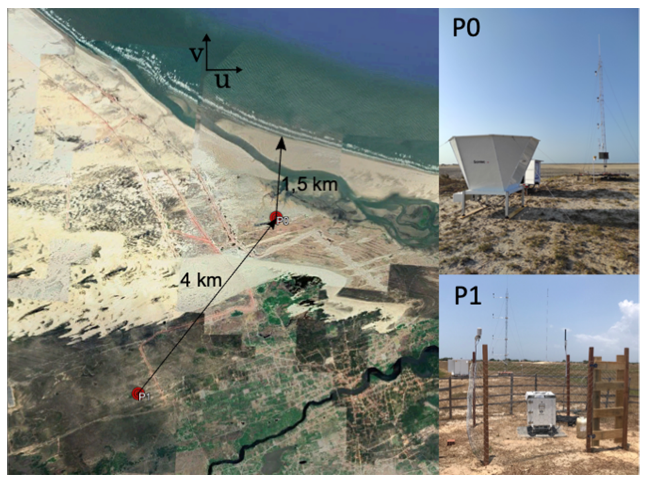
2.1. Site Description

The EOSOLAR study site is located on the eastern coast of Maranhão state, northeast Brazil, between the cities of Barreirinhas and Paulino Neves. Figure 1 illustrates with red bullets the proposed locations for micrometeorological, wind profiling, and solarimetric measurements. Stations are distributed along a transect aligned with the predominant direction of winds, that blow preferably from the NE (see the directional histogram in Figure 1). The site corresponds to a region already explored for wind energy, as shown by Figure 1, which illustrates the position of installed wind turbines.

Given the prevailing northeasterly flow, the closest station to the beach is windward of the first array of turbines. This upstream reference point P0 is 1.5 km from the ocean, so prevailing winds blow over a flat beach with very smooth terrain. Points inland from P0, and downstream of the first array of turbines, are prone to experience turbine wake effects. These points are numbered as P1, P2, P3 with increasing distance from the coast. Figure 2a illustrates a photo of the wind turbines installed over the dune field, with grass fields on the leeward side of the turbines.

Westerly winds are rare in this region, so embryo dunes generated by trade winds tend to grow and migrate inland towards the southwest, reaching up to 10 m in height (Figure 1 and Figure 2b). Over most of the terrain that will be covered by EOSOLAR stations, the ground is covered mostly by sand, grass, and low scrubs (Figure 2c,d). Small lochs can be found behind the dune fields and are more frequent in the rainy season.

The terrain has features at all length scales typically found in the coastal regions, offering a couple of advantages: it is suitable for an expansion of the wind energy potential, it can be easily accessed by road, it is suitable for micrometeorological and numerical modeling studies. Although the terrain has features at different length scales, no steep slopes are observed. The landscape is predominantly marked by gentle slopes. The vertical (rise) and the horizontal distance between the most inland point and the closest station to the beach are 15 m and 30 km respectively, resulting in a terrain slope of 0.05% (15/30,000 × 100). Locations with slopes less than 7% are considered suitable for wind exploitation [29].

During EOSOLAR’s campaigns, instruments will be installed in these different locations along the transect, for simultaneous measurements of winds and solar resources.

Figure 2. Typical landscapes for the study site. (a) Region leeward of the first array of wind turbines. (b) A well-developed dune field. (c) Grass-covered terrain. (d) Vegetated terrain.

Figure 2. Typical landscapes for the study site. (a) Region leeward of the first array of wind turbines. (b) A well-developed dune field. (c) Grass-covered terrain. (d) Vegetated terrain.

2.2. Methods and Instrumentation

The main purpose of the EOSOLAR Project is the evaluation of wind and solar resources of the state of Maranhão, combining field observations with remote sensing information, atmospheric reanalysis, and high-resolution numerical modeling. Each of the datasets delivers complementary information on the sea–land transition meteorology for estimates of wind–solar energy potential. A flowchart describing the instrumentation and procedures for solar and wind resource assessment is presented in Figure 3.

The EOSOLAR observational program, the focus of this article, is currently being carried out on Maranhão’s east coast—a region already exploited for wind power generation. Due to its outstanding renewable energy potential, instruments were deployed in the coastal region for wind data collection and assessment of the cross-shore variability of this important resource.

As the aims of this project are to assess the magnitude of changes in wind speed and turbulence induced by modifications of the terrain roughness, relief, and thermal characteristics, the EOSOLAR field program was designed specifically to characterize underlying meteorological processes that control aspects of the wind flow across this region. Equally important, solar radiation measurements were performed to track the magnitude, the time variability, and the effects of clouds over the solar resource.

This task required simultaneous measurements of different environmental parameters. Both micrometeorological variables and detailed wind profile information were necessary for the accurate characterization of the atmospheric boundary layer. Solarimetric data were crucial for a proper description of the solar resource. Table 1 lists the instruments selected for EOSOLAR field campaigns.

Two different remote sensing techniques were used for the measurement of vertical wind profiles. The first was LIDAR (Light Detection and Ranging), model Windcube V2 from Leosphere. LIDAR computes the Doppler shift from backscattered light reflected by aerosols carried in the airflow. Based on the radial velocities of five different laser beams, the equipment evaluates the wind speed vector for 20 different selected heights between 40 and 260 m above the ground level (AGL) (Table 1). The second wind profiler was SODAR (Sound Detection and Ranging), model MFAS from Scientec. Its operation is based on the reflection of acoustic pulses due to temperature inhomogeneities present in the air, with subsequent Doppler analysis. The SODAR is programmed to measure winds from 40 up to 400 m AGL with 10 m vertical resolution. Both LIDAR and SODAR provide wind averages of 10 min.

Micrometeorological instruments can provide accurate near-surface wind speeds and direction, turbulence, and flux quantities, along with other important environmental variables, such as atmospheric pressure, temperature, radiation, relative humidity, and precipitation (Table 1). Instruments were mounted over two self-supporting tipper towers of 10-m height, mounted over a road trailer for increased mobility [30,31]. For additional stability, both towers were tensioned by six sets of steel cables, attached to three horizontal legs that were fixed on the trailer base (Figure 4).

Each micrometeorological tower was equipped with a pluviometer installed at 1.5 m and a barometer and thermohydrometer at 3 m AGL. A RM Young 81,000 ultrasonic 3D anemometer was installed in each tower at 3 m AGL for the estimation of surface fluxes and turbulence. Three Gill WindSonic 75 ultrasonic 2D anemometers were installed in both towers at 5, 7, and 10 m AGL. The 3D sonic anemometer measures wind speed in three components (x-axis directed towards the East, y-axis directed towards the North, and a z-axis perpendicular and facing the zenith) and air temperature every 0.05 s (sampling frequency of 20 Hz).

All anemometers were mounted on the tower following the recommendation of Lubitz and Michalak (2018), to avoid measurements errors related to flow distortion due to the tower. Anemometers were oriented towards the prevailing winds, with a 1.5 m length boom [32].

For accurate description and comparison of wind resources along the transect, wind measurements should be performed simultaneously for different locations. As both micrometeorological data and wind profile information are necessary for meteorological characterization, the LIDAR and SODAR were always installed with an accompanied micrometeorological station. These are hereafter referred to as LIDAR-microtower and SODAR-microtower stations (Figure 3). Both sets were mounted with specifically-designed trailers for powering all the instruments and remote data communication (solar panels, batteries, power controlling unit, computer, and GSM modem) (Figure 4).

Figure 4. EOSOLAR measuring stations. From left to right: LIDAR, SODAR, and micrometeorological towers. Trailers refer to the power stations solutions (solar panels with batteries). Photo illustrates instruments mounted on the UFMA campus for the testing and intercomparison campaign (Table 2).

Figure 4. EOSOLAR measuring stations. From left to right: LIDAR, SODAR, and micrometeorological towers. Trailers refer to the power stations solutions (solar panels with batteries). Photo illustrates instruments mounted on the UFMA campus for the testing and intercomparison campaign (Table 2).

Table 1. Equipment, auxiliary instruments, variables, measuring heights and sampling frequency. AGL refers to above the ground level.

EOSOLAR Equipment	Instruments	Variables	Measurement’s Heights (AGL)	Sampling Frequency/Time-Resolution
SODAR Model: MFAS/Scintec.	--	Wind profiler: speed, direction, and turbulent intensity.	39 levels: 20 to 400 m, every 10 m.	4 s/10 min
LIDAR Model: Windcube V2/Leosphere.	Surface Comet PTH T3311 L station (pressure, temperature, and humidity).	Wind profiler: speed, direction, and turbulent intensity.	20 levels: 40 to 200 m, every 10 m. 220 to 260 m, every 20 m	5 s/10 min
Micrometeorological tower 1	Gill 1405-PK-100 Wind sonic 2D anemometer, RM Young 81,000 3D anemometer, Thermohygrometer HygroVUE10, Barometer Setra 278, Pluviometer TE525-L.	Wind speed and direction, atmospheric pressure, precipitation, temperature, and relative humidity.	3 m (sonic 3D) 5, 7, 10 m (sonic 2D)	20 Hz/10 min
Micrometeorological tower 2	Gill 1405-PK-100 Wind sonic 2D anemometer, RM Young 81,000 3D anemometer, Thermohygrometer HygroVUE10, Barometer Setra 278, Pluviometer TE525-L.	Wind speed and direction, atmospheric pressure, precipitation, temperature, and relative humidity.	3 m (sonic 3D) 5, 7, 10 m (sonic 2D)	20 Hz/10 min
Solarimetric station Model: Solys 2 Sun Tracker/Kipp & Zonen.	Pyheliometer CHP1, Pyranometer CMP10, Pyrgeometer CRG3, Gill 1405-PK-100 2D anemometer, Barometer Setra 278, Thermohygrometer HygroVUE 10, Pluviometer TE525-L.	Global Horizontal Irradiance (GHI), Direct Normal Irradiance (DNI), Diffuse Horizontal Irradiation (DHI), Global Tilted Irradiance (GTI), Outgoing Long-wave Radiation (OLR), Surface wind speed and direction, atmospheric pressure, precipitation, temperature, and relative humidity.	1.5 m	10 Hz/10 min

Table 1. Equipment, auxiliary instruments, variables, measuring heights and sampling frequency. AGL refers to above the ground level.

EOSOLAR Equipment	Instruments	Variables	Measurement’s Heights (AGL)	Sampling Frequency/Time-Resolution
SODAR Model: MFAS/Scintec.	--	Wind profiler: speed, direction, and turbulent intensity.	39 levels: 20 to 400 m, every 10 m.	4 s/10 min
LIDAR Model: Windcube V2/Leosphere.	Surface Comet PTH T3311 L station (pressure, temperature, and humidity).	Wind profiler: speed, direction, and turbulent intensity.	20 levels: 40 to 200 m, every 10 m. 220 to 260 m, every 20 m	5 s/10 min
Micrometeorological tower 1	Gill 1405-PK-100 Wind sonic 2D anemometer, RM Young 81,000 3D anemometer, Thermohygrometer HygroVUE10, Barometer Setra 278, Pluviometer TE525-L.	Wind speed and direction, atmospheric pressure, precipitation, temperature, and relative humidity.	3 m (sonic 3D) 5, 7, 10 m (sonic 2D)	20 Hz/10 min
Micrometeorological tower 2	Gill 1405-PK-100 Wind sonic 2D anemometer, RM Young 81,000 3D anemometer, Thermohygrometer HygroVUE10, Barometer Setra 278, Pluviometer TE525-L.	Wind speed and direction, atmospheric pressure, precipitation, temperature, and relative humidity.	3 m (sonic 3D) 5, 7, 10 m (sonic 2D)	20 Hz/10 min
Solarimetric station Model: Solys 2 Sun Tracker/Kipp & Zonen.	Pyheliometer CHP1, Pyranometer CMP10, Pyrgeometer CRG3, Gill 1405-PK-100 2D anemometer, Barometer Setra 278, Thermohygrometer HygroVUE 10, Pluviometer TE525-L.	Global Horizontal Irradiance (GHI), Direct Normal Irradiance (DNI), Diffuse Horizontal Irradiation (DHI), Global Tilted Irradiance (GTI), Outgoing Long-wave Radiation (OLR), Surface wind speed and direction, atmospheric pressure, precipitation, temperature, and relative humidity.	1.5 m	10 Hz/10 min

2.3. Testing and Field Campaigns

Prior to field campaigns, instruments were configured and tested on the university campus of UFMA, São Luis, Maranhão. During this period, micrometeorological towers, the SODAR, and LIDAR were mounted at a parking lot, recording data for 56 days, from 19 July to 12 September (Figure 4).

The first field campaign in the Paulino Neves region was conducted from 14 September to 8 November of 2021 (Table 2). The SODAR-microtower set was installed on point P0. The LIDAR-microtower set was positioned at station P1, both recording data for 56 days. Point P0 is 1.5 km from the beach and 4 km from point P1 (Figure 5).

P0 was initially planned as the reference point to be monitored by the SODAR-microtower station. Due to the poor signal return at this location detected on the first campaign, the SODAR-microtower set was moved inland to station P1 for the beginning of the 2nd field campaign.

As the LIDAR was more easily transported than the SODAR, the LIDAR-microtower system was transported to new locations during the subsequent campaigns, being P0 on field campaign 2 (FC2), P2 on FC3, and P3 on FC4. The SODAR-microtower remained installed on P1 for the remaining field campaigns FC2 to FC4 (Table 2).

Table 2. EOSOLAR phases of operation with a test of equipment and field campaigns, where the LIDAR-microtower and SODAR-microtower sets were moved along the station’s positions indicated in Figure 1.

EOSOLAR Phase	Begin	End	Days	Location
test and configuration	19 July 2021	12 September 2021	56	UFMA campus
field campaign 1	14 September 2021	8 November 2021	56	SODAR-microtower P0 LIDAR-microtower P1
field campaign 2	9 November 2021	13 December 2021	35	SODAR-microtower P1 LIDAR-microtower P0
field campaign 3	15 December 2021	27 January 2022	44	SODAR-microtower P1 LIDAR-microtower P2
field campaign 4	28 January 2022	Present	-	SODAR-microtower P1 LIDAR-microtower P3

Table 2. EOSOLAR phases of operation with a test of equipment and field campaigns, where the LIDAR-microtower and SODAR-microtower sets were moved along the station’s positions indicated in Figure 1.

EOSOLAR Phase	Begin	End	Days	Location
test and configuration	19 July 2021	12 September 2021	56	UFMA campus
field campaign 1	14 September 2021	8 November 2021	56	SODAR-microtower P0 LIDAR-microtower P1
field campaign 2	9 November 2021	13 December 2021	35	SODAR-microtower P1 LIDAR-microtower P0
field campaign 3	15 December 2021	27 January 2022	44	SODAR-microtower P1 LIDAR-microtower P2
field campaign 4	28 January 2022	Present	-	SODAR-microtower P1 LIDAR-microtower P3

Figure 5. Google Earth image showing the location of P0 and P1 sites for data collection.

Figure 5. Google Earth image showing the location of P0 and P1 sites for data collection.

2.4. Data Processing

2.4.1. Coordinate Rotation

Due to the three-dimensional nature of the airflow over horizontally inhomogeneous terrain or canopy (e.g., slope and ejections), the flow can be tilted with respect to the anemometer orientation [33]. In order to avoid methodological errors in mean values and flux calculations, the data needed to be rotated from the anemometer coordinate reference system to a streamlined coordinate system [34,35].

The most used coordinate rotation method, the triple rotation, is performed as three consecutive rotations, where the first rotation is done such that the x-axis is oriented along the mean wind, while the second rotation is intended to force the average vertical wind speed to be zero. The third rotation is intended to minimize the vertical momentum flux in cross-wind direction, but it is known to produce unphysical coordinate transformations and is not recommended for use in any micrometeorological calculations [36,37]. Therefore, only the double rotation of the coordinate frame over the averaging period was applied here. The streamwise coordinates were then obtained from the consecutive application of two different rotation matrices [38,39], where the first rotation turned the coordinate system around the z-axis and placed the x-axis into the direction of the mean wind:

$$\left(\begin{array}{c}ur\\ vr\\ Wr\end{array}\right)=\left(\begin{array}{ccc}\cos \mathsf{\theta }& \sin \mathsf{\theta }& 0\\ -\sin \mathsf{\theta }& \cos \mathsf{\theta }& 0\\ 0& 0& 1\end{array}\right)\left(\begin{array}{c}u\\ v\\ W\end{array}\right)$$

(1)

The new velocity components are:

$$\begin{array}{c}ur=u\cos \mathsf{\theta }+v\sin \mathsf{\theta }\\ vr=-u\sin \mathsf{\theta }+v\cos \mathsf{\theta }\\ Wr=W\end{array}$$

(2)

where the first rotation angle ($\mathsf{\theta })$ is: $\mathsf{\theta }=\arctan \left(\frac{\overline{v}}{\overline{u}}\right)$. The overline indicates the temporal average (30 min in the present work). The second rotation angle (α) is: $\mathsf{\alpha }=\arctan \left(\frac{\overline{Wr}}{\overline{ur}}\right)$ and it is around the new y-axis resulting the average vertical wind speed becomes zero (Finnigan et al., 2004) [35]:

$$\left(\begin{array}{c}u2r\\ v2r\\ W2r\end{array}\right)=\left(\begin{array}{ccc}\cos \mathsf{\alpha }& \sin \mathsf{\alpha }& 0\\ 0& 1& 0\\ -\sin \mathsf{\alpha }& 0& \cos \mathsf{\alpha }\end{array}\right)\left(\begin{array}{c}ur\\ vr\\ Wr\end{array}\right)$$

(3)

And, finally, the new velocity components to be considered after the double rotating method:

$$\begin{array}{c}u2r=ur\cos \mathsf{\alpha }+Wr\sin \mathsf{\alpha }\\ v2r=vr\\ W2r=-ur\sin \mathsf{\alpha }+Wr\cos \mathsf{\alpha }\end{array}$$

(4)

2.4.2. Calculation of Turbulence Statistics

The standardization of methodology for turbulence statistics can be facilitated with easy-to-use and freely available software. Therefore, in order to obtain quality-assured turbulent fluxes, all data from 3-D sonic anemometers were processed using the TK3 software [40]. There are several papers making use of this software [41,42,43,44], among others. Eddy-Covariance Software TK3 is a program used for calculating the surface energy fluxes and turbulence according to established literature methodologies. The program was developed in Fortran and runs on Windows and Linux platforms. For a more detailed description of the general program structure, see Mauder (2013) [45] and the user manual provided at: https://zenodo.org/record/20349#.YYfxb2DMJkh (accessed on 17 September 2021).

2.4.3. Field Intercomparison of Sonic Anemometers

Since two identical sets of sensors were hosted by the micrometeorological towers, it is worth comparing the performance of these instruments, before analyzing the fieldwork campaigns. This will assure the good agreement between instruments, through comparisons of turbulent fluctuations and time series of averaged quantities.

For this, we made use of the data collected during the configuration and testing phase (Table 2), conducted from 19 July to 12 September 2021 at the UFMA campus (Figure 4).

The instrumentation was placed in an urban region with a contrasting landscape (Figure 4). Depending on wind direction, terrain roughness and the canopy height varied substantially. Small buildings were present easterly and southeasterly from the micrometeorological towers’ positions. Small trees and bushes were present from the south to the northwest quadrant. An unobstructed landscape was present in the northeasterly direction. The site configuration, therefore, allowed investigating the sensitivity of measurements to very different landscapes.

Table 3 lists the main statistical parameter computed from the towers’ anemometers. Linear regression was applied to account for the relationship between T1 and T2 variables. Here T represents the observed variable and the numbers 1 and 2 the tower identification respectively. Root mean square error (RMSE) and bias between instruments were also evaluated (Table 3).

Towers were separated by 5 m and, in order to avoid flow distortion between neighboring towers and instruments, the set was oriented facing the prevailing winds. The measurement height of the 3-D sonic anemometers was 3 m, while it was 5 m for the 2-D sonic anemometer (only one pair of 2-D anemometers were compared). Data from all instruments were digitally recorded with synchronized time. All turbulence statistics were calculated from the 20 Hz raw data of both instruments with an averaging time of 1.0 min.

Studies for anemometers with a non-orthogonal transducer orientation [46,47,48,49,50], among others, which is the case of the RM Young 81,000 VRE (R.M. Young, Traverse City, Michigan) used here, suggests that this non-orthogonal design creates flow distortion related to the angle of attack, which is the angle between the wind vector and horizontal plane [51,52]. For quantification of this influence, comparisons between the orthogonal anemometer and/or tilted non-orthogonal anemometer are needed. This subject was out of the scope of this paper. Thus, for these initial comparisons, no angle of attack correction was applied. However, as shown by Nakai et al., (2014), one-to-one comparisons between the angle of attack corrected and uncorrected data had very high correlation coefficients (higher than 0.99) with the intercept near zero [49]. Additionally, for the friction velocity estimates from horizontal Reynold’s stress vector ($u_{\ast }={\overline{u^{\prime }{w}^{\prime }}}^2+{\overline{v^{\prime }{w}^{\prime }}}^2$)^1/4, Weber (1999) indicated that it does not depend on the coordinate system in which the vector is represented [53]. Rather, we expected the statistics between the anemometers, presented here, not to be significantly affected by non-orthogonal flow distortion as all data met the screening criteria (see Section 3.1).

Table 3. Statistics used for comparisons. T presents the variable considered, while the numbers 1 and 2 represent the tower identification. Here n represents the number of records and i is the time index. An overbar represents a time average.

Statistical Parameters	Equation
Bias	$Bias=\frac{1}{n}{\displaystyle \sum _{i=1}^n}\left(T{2}_i-T{1}_i\right)$
Root Mean Square Error	$RMSE=\sqrt{\frac{1}{n}{\displaystyle \sum _{i=1}^n}{\left(T{2}_i-T{1}_i\right)}^2}$
Pearson’s correlation coefficient	$r=\frac{{{\displaystyle \sum }}_{i=1}^n(T{1}_i-\overline{T1})(T{2}_i-\overline{T2})}{\sqrt{{{\displaystyle \sum }}_{i=1}^n{(T{2}_i-\overline{T2})}^2} \sqrt{{{\displaystyle \sum }}_{i=1}^n{(T{1}_i-\overline{T1})}^2}}$

Table 3. Statistics used for comparisons. T presents the variable considered, while the numbers 1 and 2 represent the tower identification. Here n represents the number of records and i is the time index. An overbar represents a time average.

Statistical Parameters	Equation
Bias	$Bias=\frac{1}{n}{\displaystyle \sum _{i=1}^n}\left(T{2}_i-T{1}_i\right)$
Root Mean Square Error	$RMSE=\sqrt{\frac{1}{n}{\displaystyle \sum _{i=1}^n}{\left(T{2}_i-T{1}_i\right)}^2}$
Pearson’s correlation coefficient	$r=\frac{{{\displaystyle \sum }}_{i=1}^n(T{1}_i-\overline{T1})(T{2}_i-\overline{T2})}{\sqrt{{{\displaystyle \sum }}_{i=1}^n{(T{2}_i-\overline{T2})}^2} \sqrt{{{\displaystyle \sum }}_{i=1}^n{(T{1}_i-\overline{T1})}^2}}$

3. Results and Discussion

Since all turbulent quantities consider the standard deviations of the sonic temperature, horizontal and vertical wind speed, we provide a comparative statistical analysis of all these quantities in addition to the mean wind velocities. The reasons for the observed deviations were investigated based on the turbulence and wind direction.

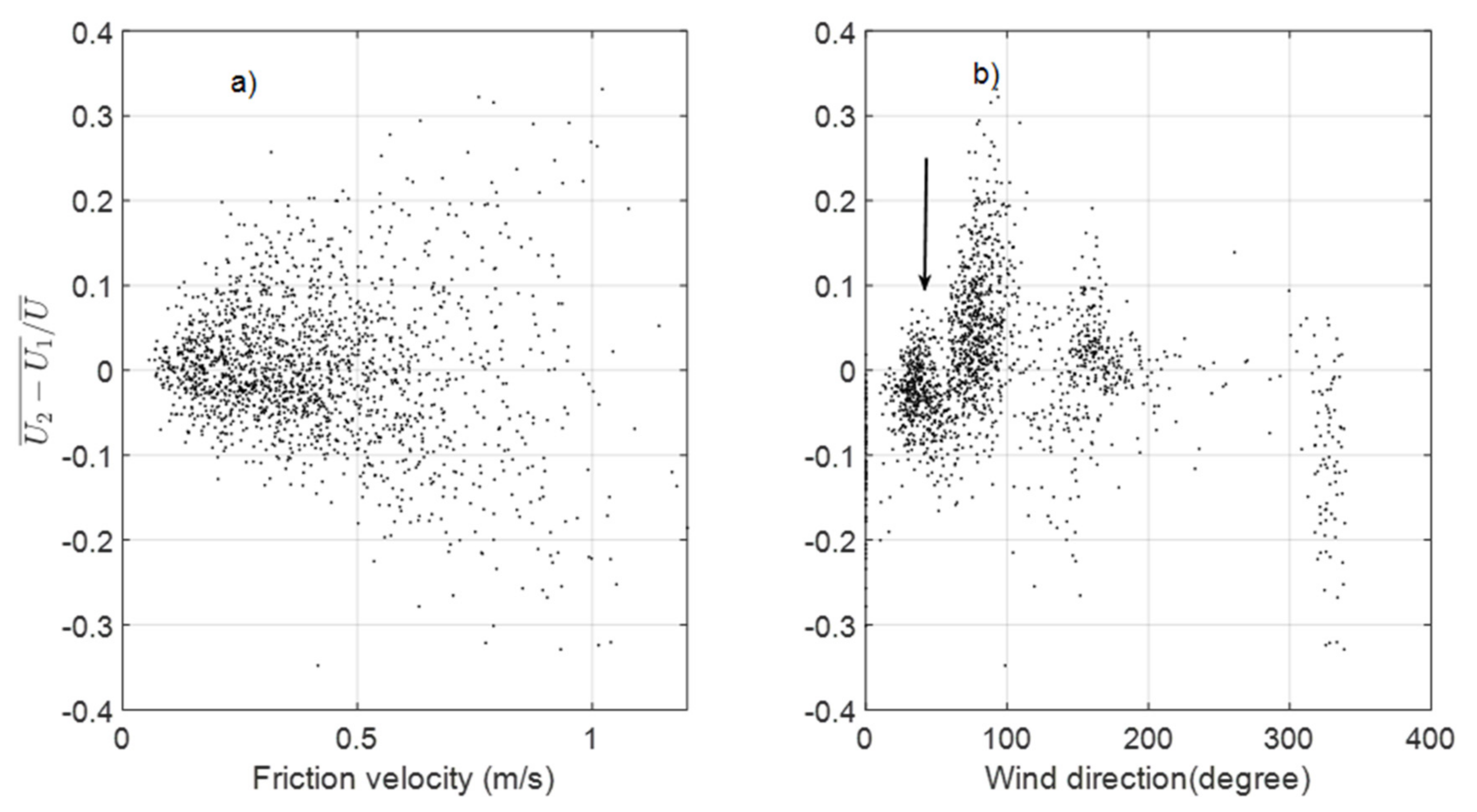
3.1. Mean and Standard Deviation of Wind Components

For the comparison of wind velocity components u, v, and w measured by the micrometeorological towers 1 and 2, the original dataset sampled at 20 Hz was reduced to a 1 min resolution time series. That means that the u, v, and w components illustrated in Figure 6 represented an average of 1200 points. The standard deviations 1 min time-series statistics presented in Table 4 were produced in a similar way, from the 20 Hz dataset.

The agreement found between anemometers was generally very good, as can be seen from Figure 5 and analyzed from Table 4 statistics. Pearson’s correlation coefficients were r = 0.87 for u component and r = 0.95 for the v component when comparing tower instruments.

There were just a few data points at wind (u component) close to 5 m s⁻¹ for which T1 presented slightly larger values than T2 (Figure 5). The v component of wind compared better, as reflected by the small regression intercept (0.00 m s⁻¹) and slopes close to one (1.06) against (−0.13 m s⁻¹) and (0.81) respectively, for the u component (Table 4). The RMSE was better for v (0.37 m s⁻¹) and biases for both were comparable, 0.27 m s⁻¹ for v and −0.23 m s⁻¹ for u (Table 4).

The 1 min standard deviations σ_u and σ_v between tower 1 and tower 2 compared better than the mean values. Biases for these two quantities (σ_u, σ_v) were 0.00 m s⁻¹ and 0.01 m s⁻¹, respectively. RMSE was 0.12 m s⁻¹ and 0.11 m s⁻¹, respectively. The Pearson’s correlation coefficient (r) ranged from 0.86 to 0.87 indicating good linearity between these measurements. This comparison was as good as that performed for two adjacent sonic anemometers in other studies, e.g., [46,54].

For the vertical component (w), the results showed an agreement of the standard deviations of the vertical velocity component (σ_w) with a RMSE of 0.08 m s⁻¹ (Table 4). Intercept and bias for (σ_w) were very small, 0.03 and 0.00 m s⁻¹, respectively, and the regression slope (0.90) and Pearson’s coefficient (r = 0.88) were close to one, suggesting a strong linear relationship between these measures. In contrast, the vertical velocity w component showed more scatter and non-linearity, with slope 0.34 and r = 0.32. This finding is in quite good agreement with the conclusion of Frank et al. (2016) [46], who suggested that these discrepancies can be explained by slight surface heterogeneities within the footprint area.

Accurate and precise measurements of the standard deviation of the vertical velocity component are required for the determination of turbulent quantities, not only for the determination of momentum flux ($u_{\ast }$) defined before. For instance, the sensible heat flux was computed from $\mathrm{H}={\rho }_a{C}_p\overline{T\prime w^{\prime }}$, where ${\rho }_a$ is the air density, Cp is the specific heat of air at constant pressure, and $\overline{T\prime w^{\prime }}$ is the covariance between the instantaneous deviation of vertical wind speed from an average value (w’), and T′ is the instantaneous deviation of air temperature from an average value. During the experiment, σ_w values ranged from 0 to 1.0 m s⁻¹ (Figure 6).

Table 4. Regression results for the comparison of the mean and standard deviation of the 3-D sonic wind velocity components, plus estimates for bias, comparability (RMSE), and Pearson’s coefficient (r).

	Slope	Intercept (m s−1)	BIAS (m s−1)	RMSE (m s−1)	r
u	0.81	−0.13	−0.23	0.42	0.87
v	1.06	0.00	0.27	0.37	0.95
σu	0.88	0.04	0.00	0.12	0.86
σv	0.91	0.05	0.01	0.11	0.87
w	0.34	−0.01	0.02	0.13	0.32
σw	0.90	0.03	0.00	0.08	0.88

Table 4. Regression results for the comparison of the mean and standard deviation of the 3-D sonic wind velocity components, plus estimates for bias, comparability (RMSE), and Pearson’s coefficient (r).

	Slope	Intercept (m s−1)	BIAS (m s−1)	RMSE (m s−1)	r
u	0.81	−0.13	−0.23	0.42	0.87
v	1.06	0.00	0.27	0.37	0.95
σu	0.88	0.04	0.00	0.12	0.86
σv	0.91	0.05	0.01	0.11	0.87
w	0.34	−0.01	0.02	0.13	0.32
σw	0.90	0.03	0.00	0.08	0.88

Discrepancies observed in these comparisons were further analyzed, investigating the relationship between the differences of instruments and potential driving variables, such as friction velocity and wind direction.

Differently from similar investigations reported in the literature, that aim to investigate different instrumental designs ([41,43,47,55], among others), we proceeded with a side-by-side comparison between two identical 3-D sonic anemometers, but subject to different upwind conditions (in terms of roughness and presence of obstacles).

There is a strong relationship between $\Delta \overline{\mathrm{U}}/\overline{\mathrm{U}}$, (relative error) with friction velocity (Figure 7a), and with the wind direction (Figure 7b). Here $\Delta \overline{\mathrm{U}}=\overline{\mathrm{U}1-\mathrm{U}2}$ represents the average difference between wind speed magnitudes, as measured by the two micrometeorological towers 1 and 2.

Maximum relative errors as a function of direction were centered at 90° and 320° due to the building wakes and high trees, respectively. The expected flow distortion for winds interacting with mounting structure (sector centered at 180°) was also evident from the large values of relative error (Figure 7b).

When the wind was aligned with the unobstructed direction (centered at 45°), a cluster of points with a low relative error was observed (see arrow in Figure 7b). The error dependence on wind direction was anticipated by Mauder et al. (2020), Grare et al. (2016), Horst et al. (2016), among others [41,48,56]. The results showed a much better agreement between the two towers for the standard deviation of the orthogonal wind components (σ_u, σ_v, σ_w), including for sonic temperature, to be presented later, in comparison with mean values.

One possibility is that all instruments were disturbed with an intensity of almost the same magnitude resulting in this good accordance in the fluctuations values, shown here. As was done in Thomas (2015) and Frank et al. (2013), for this study, no assumption was made that the two sonic anemometers were measuring exactly the same wind vectors [47,54]. Based on our results, we expected that the turbulent statistics between the towers are comparable in a physical sense since the instrument-related random uncertainty was not imperative. Lastly, we note that the intercomparison studies referred to above used an average time of 30 min for comparing anemometers, against the 1 min used here. Thus, our results can be considered as a conservative estimate for the systematic error between the two towers.

Figure 7. Differences in wind velocity measurements between the two towers normalized by the mean wind velocity versus the friction velocity (a) and wind direction (b). Arrow indicates the unobstructed direction.

Figure 7. Differences in wind velocity measurements between the two towers normalized by the mean wind velocity versus the friction velocity (a) and wind direction (b). Arrow indicates the unobstructed direction.

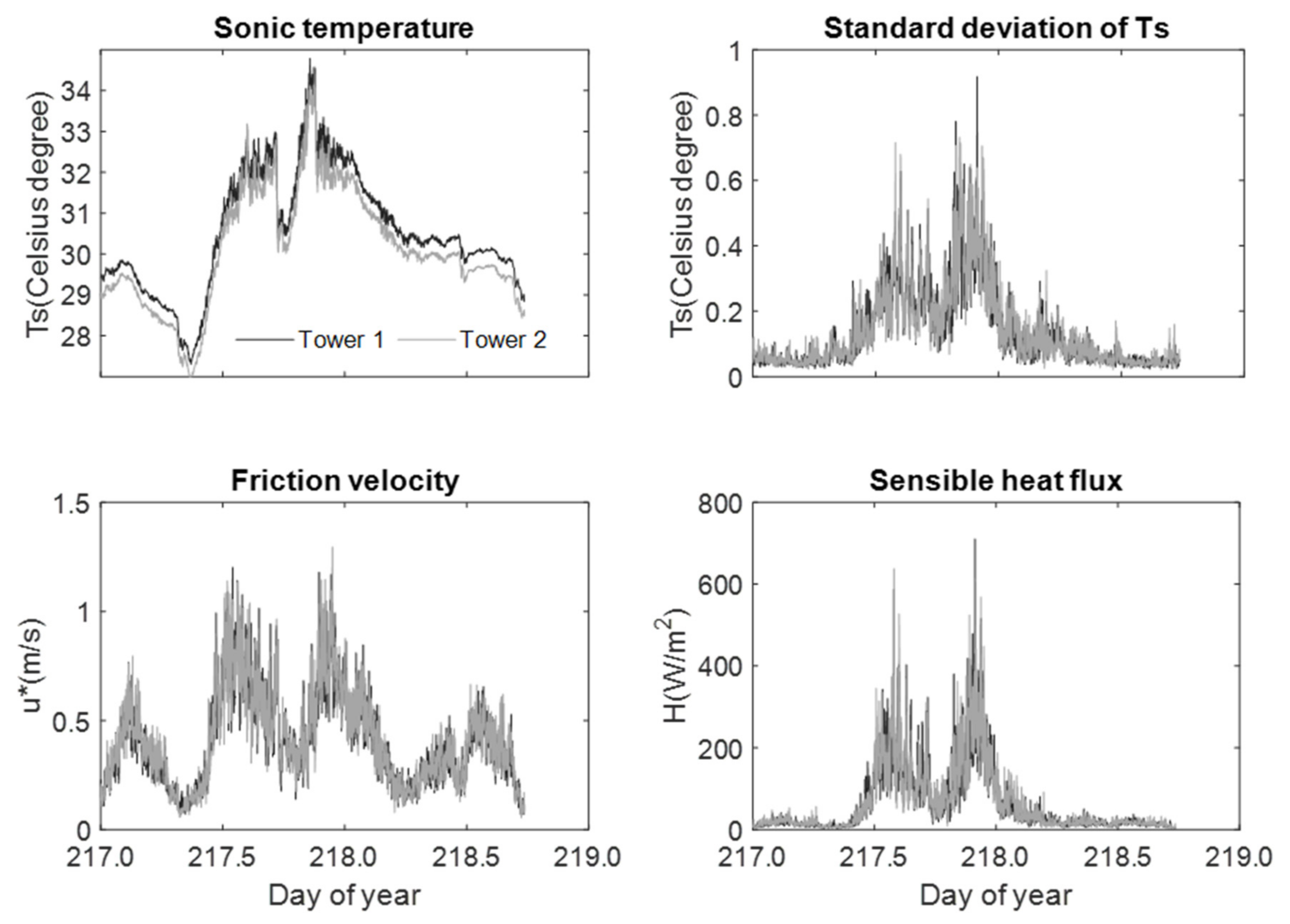
3.2. Statistical Analysis of the Comparison for the Turbulence Quantities

Statistical analysis and regression parameters for sonic temperature (Ts), friction velocity (u_*), and sensible heat flux (H), generally showed a good agreement between the tower 1 and tower 2 measurements (Figure 8, Table 5).

Particularly, the measurements of the friction velocity ranged from 0.2 to 1.3 m s⁻¹. The statistical comparison between friction velocity from the micrometeorological towers 1 and 2 showed a slight difference, with a regression slope of 0.96, a Pearson’s coefficient (r) of 0.94, bias of 0.00 m s⁻¹, RMSE of 0.07 m s⁻¹. Tower 1 underestimated friction velocity compared to tower 2 by 4%.

This is somewhat unexpected because previous studies [41] indicated that friction velocity would be typically more difficult to measure due to the spectral separation between the peaks in u and w spectra. Nevertheless, the comparability between the two towers of these values was surprisingly good.

In contrast, the sonic temperature measurements of the two towers, despite the very good regression statistics, showed a large bias (−0.42 °C) and RMSE (0.42 °C). This high difference between measures is not so unexpected since the accuracy informed at the specification technical note was ±2 °C (0 to 30 m s⁻¹ wind) (R.M. Young, technical report). This offset in mean temperature was large enough to impact calculations of air density and other parameters that are temperature-dependent. So, an independent measurement of the mean temperature from Rotronic Instruments with an accuracy of ±0.3 °C will be used for the EOSOLAR Project. On the contrary, the σTs for both anemometers compared very well with a slope of 0.93 and bias and RMSE of 0.00 °C and 0.05 °C, respectively. As the turbulence parameters were obtained from these fluctuating values we expect the turbulent statistics between the anemometer, including fluxes, to agree well.

The diurnal evolution of sensible heat fluxes (H) is shown in Figure 8. During the measurement period, H ranged from near 0 to about 600 W m⁻² (flux away from the surface was positive), evidencing the enhanced heat flux at the equatorial region. This parameter for the two towers compared very well, with slope, bias, and r of 0.92, 1.84, and 0.9, respectively (Table 5). All these intercomparisons demonstrated very good consistency between the tower’s instruments.

Figure 8. Comparison between 3-D sonic anemometers for micrometeorological tower 1 (black curves) and 2 (gray curves). Averaging time was 1.0 min with a sampling rate of 20 Hz.

Figure 8. Comparison between 3-D sonic anemometers for micrometeorological tower 1 (black curves) and 2 (gray curves). Averaging time was 1.0 min with a sampling rate of 20 Hz.

Table 5. Regression results for the comparison of the turbulent quantities of sonic temperature (Ts), standard deviation of Ts (σ_Ts), friction velocity (u*), and turbulent heat fluxes (H), plus estimates for bias, comparability (RMSE), and Pierson’s coefficient (r).

	Slope	Intercept	BIAS	RMSE	r
Ts (°C)	1.01	−0.03	−0.42	0.42	0.99
σTs (°C)	0.93	0.01	0.00	0.05	0.91
u* (m s−1)	0.96	0.02	0.00	0.07	0.94
H (W m−2)	0.92	6.90	1.84	35.69	0.91

Table 5. Regression results for the comparison of the turbulent quantities of sonic temperature (Ts), standard deviation of Ts (σ_Ts), friction velocity (u*), and turbulent heat fluxes (H), plus estimates for bias, comparability (RMSE), and Pierson’s coefficient (r).

	Slope	Intercept	BIAS	RMSE	r
Ts (°C)	1.01	−0.03	−0.42	0.42	0.99
σTs (°C)	0.93	0.01	0.00	0.05	0.91
u* (m s−1)	0.96	0.02	0.00	0.07	0.94
H (W m−2)	0.92	6.90	1.84	35.69	0.91

3.3. Comparisons of Observed Wind Profiles from LIDAR and SODAR

The continuous development of larger wind turbines required taller meteorological masts to cover the increasing rotor heights, with more instruments to properly sample the atmospheric flow. Constructing tall masts at multiple locations for wind resource characterization is becoming difficult logistically and is cost prohibitive.

LIDAR and SODAR have been intensively applied in wind energy research projects, as a solution to this problem. These remote sensing instruments can measure winds from 40 to 300 m in many different levels, with very good vertical resolution. They are more easily transported between different locations, and easily configured for sampling from 20 up to 40 levels (Table 1). The EOSOLAR project makes use of these different technologies, so an intercomparison of the instruments is justified. This testing campaign for equipment validation was conducted on the UFMA campus from 19 July to 12 September 2021 (Table 2, Figure 4).

Figure 9 shows the mean wind profile of wind speed measured by the co-located LIDAR and SODAR. The agreement between wind speeds from the LIDAR and SODAR was excellent at 100 m (the hub height). SODAR observations showed slightly lower wind speeds from 50 up to 100 m. SODAR to LIDAR differences decreased with height and invert beyond 130 m. Averaging all days, we found that below 130 m the bias was generally negative (max of 0.70 m s⁻¹), while in the upper levels (higher than 130 m), the bias was positive, although smaller (lower than 0.50 m s⁻¹) (Figure 9).

This result agrees with Bradley et al. (2007) [57], who noted that LIDAR performs similarly to SODAR. The larger bias in lower heights (Figure 9a) has been attributed to the horizontal shear evident in the complex terrain [58,59,60]. This finding was substantiated by the conclusions of Bradley (2008) [59], who related this bias with the conical scan used by the LIDAR, which results in the three wind components being determined from spatially separated volumes of air (and because of this, reduced performance in complex terrain would be expected for lower heights). Another possibility could be due to the working principle of the SODAR that is based on density fluctuations related to the thermal structure of the atmosphere [61]. Since sea–land breeze is important in our study site, the inversion in the bias tendency with the height could be related to this mesoscale feature. Similar results were found in the Central Mediterranean, where Lo Feudo et al. (2020) argued that the main hypothesis is that during the breeze events, the concentration of aerosols in the vertical layer is not homogeneous; therefore, the LIDAR signal is weak [62].

SODAR and LIDAR time-series correlation, as a function of height, are shown in Figure 9b. Here correlations were computed for the zonal u and meridional v components separately. The series correlated at r = 0.99 from 100 to 150 m AGL, with values also higher than 0.97 above 150 m. Correlation decayed faster for lower levels, reaching 0.90 below 50 m height.

Figure 9. (a) Vertical profiles of wind speed measured by LIDAR and SODAR. (b) Vertical distribution of the Pearson’s correlation coefficient comparing LIDAR and SODAR in terms of their zonal and meridional wind components.

Figure 9. (a) Vertical profiles of wind speed measured by LIDAR and SODAR. (b) Vertical distribution of the Pearson’s correlation coefficient comparing LIDAR and SODAR in terms of their zonal and meridional wind components.

3.4. Hourly Wind Evolution during Local Flow: Surface Station and LIDAR Complementarity

During the first field campaign at Barreirinhas, on the morning of 21 September 2021, a meteorological phenomenon, characterized by a sudden decrease in wind speed and a sharp change in its direction, was registered both at the surface station and LIDAR profiler (Table 2). The abrupt reduction in wind speeds resulted in an operational disruption of a large wind power plant close to our site, during this event.

Here this phenomenon is investigated combining the micrometeorological tower and the LIDAR wind profiler data. The first part of the analysis was performed with the micrometeorological tower dataset, selecting five days, including 21 September (disturbance period) (Figure 10 and Figure 11).

At the same time, the evolution of wind speed and direction at different heights was provided by LIDAR (Figure 12). Days, 19, 20, 22, and 23 September, represent the expected wind behavior in this region.

As shown by Hara et al. (2012), a sudden wind loss can cause significant variability in drivetrain loads and a reduction in the expected life of drivetrain components [63]. Therefore, the early detection of this kind of phenomenon would make it possible to notify the wind farm about the occurrence of this type of meteorological phenomenon in advance, which would facilitate the management of the wind farm. The underlying physics and synoptic conditions during this event are not in the scope of this article. The topic is under investigation, and it will be communicated later as a practical example of nowcasting.

First, we will concentrate on the description and discussion on the mean conditions. The time series of wind speed, wind direction, air temperature, relative humidity, and atmospheric pressure are shown in Figure 10. For the expected conditions for the dry season (an exception to 21 September), wind presented a marked diurnal variability. Speeds increased rapidly from 6 m s⁻¹ at 00:00 h to a maximum of 12 m s⁻¹ at 12:00 h and early afternoon. Winds decreased between late afternoon and midnight 00:00. The wind direction (Figure 10b) reflected the changes in wind speed with the winds blowing from the east (90°) when the winds were strongest and shifting to the northeast during lower speeds. At the site, temperature (humidity) exhibited a maximum (minimum) around the central hours of the days (Figure 10c,d). The diurnal changes in wind speed during the sea breeze cycle reflected changes in pressure. The two daily maxima in atmospheric pressure corresponded to maxima in wind speed in the morning and the decrease in speeds in the night (Figure 10e). According to Sakazaki and Hamilton (2017), this daily cycle is a manifestation of the atmospheric solar tide, which is caused by solar heating of the stratosphere, troposphere, and surface, and appears in the pressure data as primary and secondary maxima [64].

Figure 11 illustrates the vertically averaged (3, 5, 7, and 10 m) wind speeds and direction, comparing the 21 September event with the expected wind behavior in this location.

Figure 10. Time series over the period of 19 to 23 of September for (a) wind speed; (b) wind direction; (c) air temperature; (d) relative humidity; and (e) atmospheric pressure. A vertical dashed bar indicates the meteorological phenomenon of interest (21 September, between 07:00 h and 08:30 h LT).

Figure 10. Time series over the period of 19 to 23 of September for (a) wind speed; (b) wind direction; (c) air temperature; (d) relative humidity; and (e) atmospheric pressure. A vertical dashed bar indicates the meteorological phenomenon of interest (21 September, between 07:00 h and 08:30 h LT).

Figure 11. Diurnal variability of the vertically averaged wind speed (a) and wind direction (b). Tower anemometers at 3, 5, 7, and 10 m were used for the vertical averages. A black line illustrates the time series for 21 September, with two vertical dashed lines indicating the meteorological phenomenon of interest (21 September, between 07:00 h and 08:30 h LT). A gray line represents the expected daily wind behavior (computed for 24 h with 1 min time resolution).

Figure 11. Diurnal variability of the vertically averaged wind speed (a) and wind direction (b). Tower anemometers at 3, 5, 7, and 10 m were used for the vertical averages. A black line illustrates the time series for 21 September, with two vertical dashed lines indicating the meteorological phenomenon of interest (21 September, between 07:00 h and 08:30 h LT). A gray line represents the expected daily wind behavior (computed for 24 h with 1 min time resolution).

Figure 12. Data time series: (a) Magnitude of wind speed (m s⁻¹) based on 20 observations of LIDAR with height (40 to 260 m). Vertical profile of (b) wind speed (m s⁻¹), and (c) direction (degrees). Here the angle represents the direction that the wind is blowing from (in reference to the true north). Time is expressed in local time.

Figure 12. Data time series: (a) Magnitude of wind speed (m s⁻¹) based on 20 observations of LIDAR with height (40 to 260 m). Vertical profile of (b) wind speed (m s⁻¹), and (c) direction (degrees). Here the angle represents the direction that the wind is blowing from (in reference to the true north). Time is expressed in local time.

The diurnal cycle of wind speeds showed a wind range of 6.0 m s⁻¹, with a minimum of 4.0 m s⁻¹ just after sunset, after having descended from its maximum value of 10 m s⁻¹ observed between 10:00 h and 14:00 h (Figure 11a). The diurnal cycle of wind intensity (Figure 11a) and direction (Figure 11b) was consistent with a breeze signal forced by a differential heating of the surface air above the sea and over land. Medeiros et al. (2021) [65] studied the low-level atmospheric flow at the Central North Coast of Brazil and showed that the breeze circulation is most intense in the eastern part of Maranhão state. As shown by these authors (see Figure 6 in Medeiros et al., 2021) [65], at the end of the night and early morning (06:00 h–08:00 h), the surface air over the land was cooler than the air over the sea and warmer during the afternoon. Around morning (07:00 h–09:00 h), an easterly flow was present in contrast to the expected northeasterly trade wind (dashed bar in Figure 10 and Figure 11). The combination of the land breeze (week southwesterly flow) during this period and the trade wind (strong northeasterly wind) would result in this observed clockwise wind deviation, a mechanism such as that used by Pattiaratchi et al. (1997) [66], explaining the shore-parallel sea breeze on the Australian coast. Note that the expected northeasterly sea breeze during the late morning and afternoon enhances the trade wind resulting in intensified wind speeds (Figure 11a).

This short-duration (07:00 h–08:30 h) meteorological phenomenon, characterized by a sudden decrease in wind speed and a sharp change in its direction observed on the morning of 21 September 2021, was registered by the surface instrumentation (Figure 11) and by the wind profiler (LIDAR) (Figure 12), confirming the evolution of winds at all heights.

The sudden wind loss (~40% of reduction) (Figure 11a) and the sharp deviation southeastward in the direction (Figure 11b) are relevant not only for wind energy but also to the dispersion of pollutants, coastal ocean circulation, navigation, and sand transport. During this event, a deviation in both temperature and humidity, related to a normal diurnal cycle (mean conditions in Figure 10c,d), was observed. The temperature (humidity) stopped rising (lowering) at around 07:00 h reaching values of 1 °C (7%) lower (higher) than mean values for the period. These results once again confirmed that the high-resolution meteorological measures are essential to predict the local wind features. The scale of the process presented here (minutes to an hour) anticipates its importance to understanding the ramping features in netload since due to dramatic change both in intensity and direction, wind down- and up-ramps are expected to occur during this type of event.

4. Conclusions and Future Work

The EOSOLAR Project is producing an excellent dataset of the atmospheric boundary-layer flow of the northeast Brazil equatorial coastal zone. The field campaign will provide valuable information for scientific research, model parameterizations, and planning future wind farms. These will include details of time variation in mean wind speed along with landscape-induced spatial variations of various turbulence characteristics and their implications to wind power. The results will be extremely useful for the validation and improvement in physical and numerical models of the atmospheric flow. This article described EOSOLAR’s overall objectives, together with the physical characteristics of the study region and the necessary methods and instrumentation to study the wind and solar resource variability.

In order to evaluate the consistency between instruments hosted at the two micrometeorological towers, a side-by-side comparison between two identical 3-D sonic anemometers, but subject to different upwind footprint surroundings, was performed. Generally, biases and regression intercepts were very small for all sensors and all computed variables. The results showed that the turbulent statistics between the towers were comparable in a physical sense since the random instrument-related uncertainty was not imperative.

As the turbulence parameters obtained from fluctuating variables were similar, the turbulent statistics between anemometers, including fluxes, agreed well. The observed consistency between the towers is necessary for conducting intercomparisons studies planned for the field campaigns. Comparisons between mean vertical profiles of wind speed measured by the co-located LIDAR and SODAR pointed out the excellent agreement between measurements at 100 m (the hub height).

A short-duration (07:00 h–08:30 h) meteorological phenomenon, characterized by a sudden decrease in wind speed and a sharp change in its direction, was registered both at the surface station and wind profile from LIDAR in the first field campaign. This sharp reduction in the wind speed resulted in an operational disruption of a large wind power plant close to our site, during the event duration. Measurements from both the 2-D and 3-D anemometers and the LIDAR registered this phenomenon.

A preliminary analysis of the diurnal cycle confirmed the results of Medeiros et al. (2021), Souza and Oyama (2017), and Medeiros and Fisch (2012) [20,21,65], which demonstrated that the sea breeze contributes to reinforcing the synoptic flow, while the land breeze is overridden by the stronger synoptic flow that blows from the opposite direction.

The large decrease in wind magnitude and time scale (hours) associated with the event described on 21 September 2021 anticipate the need to better understand the frequency of occurrence of this type of phenomenon and access its overall impact on the wind park power ramps. The underlying physics and synoptic conditions controlling this event are under investigation and will be communicated later.

References

1. Lucena, J.A.Y.; Lucena, K.A.A. Wind energy in Brazil: An overview and perspectives under the triple bottom line. Clean Energy 2019, 3, 69–84. [Google Scholar] [CrossRef] [Green Version]
2. Brannstrom, C.; Gorayeb, A.; de Souza, W.F.; Leite, N.S.; Chaves, L.O.; Guimarães, R.; Gê, D.R.F. Perspectivas geográficas nas transformações do litoral brasileiro pela energia eólica. Rev. Bras. Geogr. 2018, 63, 3–28. [Google Scholar] [CrossRef] [Green Version]
3. Pimenta, F.M.; Kempton, W.; Garvine, R. Combining meteorological stations and satellite data to evaluate the offshore wind power resource of Southeastern Brazil. Renew. Energy 2008, 33, 2375–2387. [Google Scholar] [CrossRef]
4. Lima, D.K.S.; Leão, R.P.S.; dos Santos, A.C.S.; de Melo, F.D.C.; Couto, V.M.; de Noronha, A.W.T.; Oliveira, D.S. Estimating the offshore wind resources of the State of Ceará in Brazil. Renew. Energy 2015, 83, 203–221. [Google Scholar] [CrossRef]
5. Pimenta, F.M.; Silva, A.R.; Assireu, A.T.; Almeida, V.S.; Saavedra, O.R. Brazil Offshore Wind Resources and Atmospheric Surface Layer Stability. Energies 2019, 12, 4195. [Google Scholar] [CrossRef] [Green Version]
6. De Azevedo, S.S.P.; Júnior, A.O.P.; Da Silva, N.F.; Araújo, R.S.B.; Júnior, A.A.C. Assessment of Offshore Wind Power Potential along the Brazilian Coast. Energies 2020, 13, 2557. [Google Scholar] [CrossRef]
7. Balthermie, R.J. The effects of atmospheric stability on coastal wind climates. Meteorol. Appl. 1999, 6, 39–47. [Google Scholar]
8. Garratt, J.R. The Atmospheric Boundary Layer; Cambridge Atmospheric and Space Science Series; Cambridge University Press: Cambridge, UK, 1992; p. 316. [Google Scholar]
9. Wang, H.; Barthelmie, R.J.; Crippa, P. Profiles of Wind and Turbulence in the Coastal Atmospheric Boundary Layer of Lake Erie. J. Phys. Conf. Ser. 2014, 524, 012117. [Google Scholar] [CrossRef] [Green Version]
10. Moriarty, P.; Nicholas, H.; Debnath, M.; Herges, T.; Isom, B.; Lundquist, J.K.; Maniaci, D.; Naughton, B.; Pauly, R.; Roadman, J.; et al. American WAKE Experiment (AWAKEN); National Renewable Energy Laboratory: Golden, CO, USA, 2020; NREL/TP-5000-75789.
11. Santos, P.; Mann, J.; Vasiljević, N.; Cantero, E.; Sanz Rodrigo, J.; Borbón, F.; Martínez-Villagrasa, D.; Martí, B.; Cuxart, J. The Alaiz experiment: Untangling multi-scale stratified flows over complex terrain. Wind. Energ. Sci. 2020, 5, 1793–1810. [Google Scholar] [CrossRef]
12. Fernando, H.J.S.; Mann, J.; Palma, J.M.; Lundquist, J.K.; Barthelmie, R.J.; Belo-Pereira, M.; Brown, W.O.; Chow, F.K.; Gerz, T.; Hocut, C.M.; et al. The Perdigão: Peering into Microscale Details of Mountain Winds. Bull. Am. Meteorol. Soc. 2019, 100, 799–819. [Google Scholar] [CrossRef]
13. Karagali, I.; Mann, J.; Dellwik, E.; Vasiljevic, N. New European Wind Atlas: The Østerild balconies experiment. J. Physics Conf. Ser. 2018, 1037, 052029. [Google Scholar] [CrossRef] [Green Version]
14. Shaw, W.J.; Pekour, M.S.; Newsom, R.K. Lidar Buoy Data Analysis: Basic Assessment of Observed Conditions and Instrument Performance Off Virginia and New Jersey; Pacific Northwest National Lab. (PNNL): Richland, WA, USA, 2018.
15. Standridge, C.R.; Zeitler, D.; Clark, A.; Spoelma, T.; Nordman, E.E.; Boezaart, T.A.; Edmonson, J.; Howe, G.; Meadows, G.; Cotel, A.; et al. Lake Michigan Wind Assessment Analysis 2012 and 2013. Int. J. Renew. Energy Dev. 2017, 6, 19–27. [Google Scholar] [CrossRef] [Green Version]
16. Berg, J.; Mann, J.; Bechmann, A.; Courtney, M.S.; Jørgensen, H.E. The Bolund Experiment, Part I: Flow Over a Steep, Three-Dimensional Hill. Bound.-Layer Meteorol. 2011, 141, 219–243. [Google Scholar] [CrossRef] [Green Version]
17. Taylor, P.A.; Teunissen, H.W. The Askervein Hill project: Overview and background data. Bound.-Layer Meteorol. 1987, 39, 15–39. [Google Scholar] [CrossRef]
18. Germano, M.F.; Oyama, M.D. Local circulation features in the Eastern Amazon: High-resolution simulation. J. Aerosp. Technol. Manag. 2020, 12, 1–16. [Google Scholar]
19. Souza, D.C.; Oyama, M.D. Breeze potential along the Brazilian Northern and Northeastern Coast. J. Aerosp. Technol. Manag. 2017, 9, 368–378. [Google Scholar] [CrossRef]
20. Medeiros, L.E.; Fisch, G. Low atmospheric flow at Centro de Lançamento de Alcântara (CLA) and surrounding areas of the north part of the Maranhão State. In Proceedings of the XVII Congresso Brasileiro de Meteorologia, Gramado, Brazil, 23–28 September 2012. [Google Scholar]
21. Ramalho, K.A.C.; Oyama, M.D. Five-day Cycle of the Surface Wind in the Alcântara Launch Center During the Dry Quarter. Mod. Environ. Sci. Eng. 2020, 6, 84–98. [Google Scholar]
22. Medeiros, L.E.; Magnago, R.O.; Fisch, G.; Marciotto, E.R. Observational study of the surface layer at an ocean-land transition region. J. Aerosp. Technol. Manag. 2013, 4, 449–458. [Google Scholar] [CrossRef]
23. Marciotto, E.R.; Fisch, G. Investigation of approaching ocean flow and its interaction with land internal boundary layer. Am. J. Environ. Eng. 2013, 1, 18–23. [Google Scholar] [CrossRef] [Green Version]
24. Pereira, I.; Fisch, G.F.; Miranda, I.; Machado, L.A.T.; Alves, M.A.S. Atlas Climatológico do Centro de Lançamento de Alcântara; Technical Report; Centro Técnico Aeroespacial: São José dos Campos, SP, Brazil, 2002.
25. Oliveira, F.P.; Oyama, M.O. Squall-line initiation over the northern coast of Brazil in March: Observational features. Meteor. Appl. 2019, 27, e1799. [Google Scholar] [CrossRef]
26. Schuch, D.; Fisch, G. The use of an atmospheric model to simulate the rocket exhaust effluents transport and dispersion for the Centro de Lançamento de Alcântara. J. Aerosp. Technol. Manag. 2017, 2, 137–146. [Google Scholar] [CrossRef]
27. Silva, A.F.G.; Fisch, G. Avaliação do Modelo WRF para a Previsão do Perfil do Vento no Centro de Lançamento de Alcântara. Rev. Bras. Meteorol. 2014, 29, 259–270. [Google Scholar] [CrossRef]
28. Avelar, A.C.; Brasileiro, F.L.C.; Marto, A.G.; Marciotto, E.R.; Fisch, G.; Faria, A.F. Wind tunnel simulation of the atmospheric boundary layer for studying the wind pattern at Centro de Lançamento de Alcântara. J. Aerosp. Technol. Manag. 2012, 4, 463–473. [Google Scholar] [CrossRef] [Green Version]
29. Rodman, L.C.; Meentemeyer, R.K. A geographic analysis of wind turbine placement in Northern California. Energy Policy 2006, 34, 2137–2149. [Google Scholar] [CrossRef]
30. De Boer, G.; Erwin, A.; Borenstein, S.; Dixon, C.; Shanti, W.; Houston, A.; Argrow, B. Measurements from mobile surface vehicles during the lower atmospheric profiling studies at elevation—A remotely-piloted aircraft team experiment (LAPSE-RATE). Atmos. Meas. Tech. 2014, 7, 1825–1837. [Google Scholar] [CrossRef]
31. Belusic´, D.; Lenschow, D.H.; Tapper, N.J. Performance of a mobile car platform for mean wind and turbulence measurements. Atmos. Meas. Tech. 2014, 7, 1825–1837. [Google Scholar] [CrossRef] [Green Version]
32. Lubitz, W.D.; Michalak, A. Experimental and theoretical investigation of tower shadow impacts on anemometer measurements. J. Wind Eng. Indust. Aerod. 2018, 176, 112–119. [Google Scholar] [CrossRef]
33. Bohrer, G.; Katul, G.; Walko, R.L.; Avissar, R. Exploring the Effects of Microscale Structural Heterogeneity of Forest Canopies Using Large-Eddy Simulations. Bound.-Layer Meteorol. 2009, 132, 351–382. [Google Scholar] [CrossRef]
34. Finnigan, J.J.; Clement, R.; Malhi, Y.; Leuning, R.; Cleugh, H.A. A Re-Evaluation of Long-Term Flux Measurement Techniques Part I: Averaging and Coordinate Rotation. Bound.-Layer Meteorol. 2003, 107, 1–48. [Google Scholar] [CrossRef]
35. Finnigan, J.J. A re-evaluation of long-term flux measurement techniques—Part II: Coordinate systems. Bound.-Layer Meteorol. 2004, 113, 1–41. [Google Scholar] [CrossRef]
36. Klipp, C. Turbulent friction velocity calculated from the Reynolds stress tensor. J. Amosph. Sci. 2018, 75, 1837–1942. [Google Scholar] [CrossRef]
37. Sun, J. Tilt corrections over complex terrain and their implication for CO2 transport. Bound.-Layer Meteorol. 2007, 124, 143–159. [Google Scholar] [CrossRef]
38. Golzio, A.; Bollati, I.M.; Ferrarese, S. An Assessment of Coordinate Rotation Methods in Sonic Anemometer Measurements of Turbulent Fluxes over Complex Mountainous Terrain. Atmosphere 2019, 10, 324. [Google Scholar] [CrossRef] [Green Version]
39. Foken, T. Micrometeorology, 2nd ed.; Springer: Berlin/Heidelberg, Germany, 2016. [Google Scholar]
40. Mauder, M.; Foken, T. Eddy-Covariance Software TK3. 2015. Available online: https://0-doi-org.brum.beds.ac.uk/10.5281/zenodo.20349 (accessed on 17 September 2021).
41. Mauder, M.; Eggert, M.; Gutsmuths, C.; Oertel, S.; Wilhelm, P.; Voelksch, I.; Wanner, L.; Tambke, J.; Bogoev, I. Comparison of turbulence measurements by a CSAT3B sonic anemometer and a high-resolution bistatic Doppler lidar. Atmos. Meas. Tech. 2020, 13, 969–983. [Google Scholar] [CrossRef] [Green Version]
42. Goeckede, M.; Kittler, F.; Schaller, C. Quantifying the impact of emission outbursts and non-stationary flow on eddy-covariance CH4 flux measurements using wavelet techniques. Biogeosciences 2019, 16, 3113–3131. [Google Scholar] [CrossRef] [Green Version]
43. Mauder, M.; Zeeman, M.J. Field intercomparison of prevailing sonic anemometers. Atmos. Meas. Tech. 2018, 11, 249–263. [Google Scholar] [CrossRef] [Green Version]
44. Mammarella, I.; Peltola, O.; Nordbo, A.; Järvi, L.; Rannik, Ü. Quantifying the uncertainty of eddy covariance fluxes due to the use of different software packages and combinations of processing steps in two contrasting ecosystems. Atmos. Meas. Tech. 2016, 9, 4915–4933. [Google Scholar] [CrossRef] [Green Version]
45. Mauder, M.; Cuntz, M.; Drüe, C.; Graf, A.; Rebmann, C.; Schmid, H.P.; Schmidt, M.; Steinbrecher, R. A strategy for quality and uncertainty assessment of long-term eddy-covariance measurements. Agric. For. Meteorol. 2013, 169, 122–135. [Google Scholar] [CrossRef]
46. Frank, J.M.; Massman, W.J.; Swiatek, E.; Zimmerman, H.A.; Ewers, B.E. All sonic anemometers need to correct for transducer and structural shadowing in their velocity measurements. J. Atmos. Ocean. Technol. 2016, 33, 149–167. [Google Scholar] [CrossRef] [Green Version]
47. Thomas, T. Three-Dimensional Wind Speed and Flux Measurements over a Rain-Fed Soybean Field Using Orthogonal and Non-Orthogonal Sonic Anemometer Designs. Master’s Thesis, Dissertations & Theses in Natural Resources. University of Nebraska, Lincoln, NE, USA, 2015; p. 128. [Google Scholar]
48. Horst, T.W.; Semmer, S.R.; Maclean, G. Correction of a Non-orthogonal, Three-Component Sonic Anemometer for Flow Distortion by Transducer Shadowing. Bound.-Layer. Meteorol. 2015, 155, 371–395. [Google Scholar] [CrossRef] [Green Version]
49. Nakai, T.; Iwata, H.; Harazono, Y.; Ueyama, M. An inter-comparison between Gill R3 and campbell sonic anemometers. Agric. For. Meteorol. 2014, 195, 123–131. [Google Scholar] [CrossRef]
50. Nakai, T.; Shimoyama, K. Ultrasonic anemometer angle of attack errors under turbulent conditions. Agric. For. Meteorol. 2012, 162, 14–26. [Google Scholar] [CrossRef] [Green Version]
51. Christen, A.; Gorsel, E.; Andretta, M.; Calanca, P.; Rotach, M.W.; Vogt, R. Intercomparison of ultrasonic anemometers during the map Riviera project. In Proceedings of the Ninth Conference Mountain Meteorology, Snowmass Village, CO, USA, 7–12 August 2000. [Google Scholar]
52. Gash, J.; Dolman, A. Sonic anemometer (co) sine response and flux measurement: I. the potential for (co) sine error to affect sonic anemometer-based flux measurements. Agric. For. Meteorol. 2003, 119, 195–207. [Google Scholar] [CrossRef]
53. Weber, R.O. Remarks on the Definition and Estimation of Friction Velocity. Bound.-Layer Meteorol. 1999, 93, 197–209. [Google Scholar] [CrossRef]
54. Frank, J.M.; Massman, W.J.; Ewers, B.E. Underestimates of sensible heat flux due to vertical velocity measurement errors in non-orthogonal sonic anemometers. Agric. For. Meteorol. 2013, 171, 72–81. [Google Scholar] [CrossRef]
55. Huq, S.; De Roo, F.; Foken, T.; Mauder, M. Evaluation of probe-induced flow distortion of Campbell CSAT3 sonic anemometers by numerical simulation. Bound.-Layer Meteorol. 2017, 164, 9–28. [Google Scholar] [CrossRef]
56. Grare, L.; Lenain, L.; Melville, W.K. The Influence of Wind Direction on Campbell Scientific CSAT3 and Gill R3-50 Sonic Anemometer Measurements. J. Atmos. Ocean. Technol. 2016, 33, 2477–2497. [Google Scholar] [CrossRef] [Green Version]
57. Bradley, S.; von Hünerbein, S. Comparisons of New Technologies for Wind Profile Measurements Associated with Wind Energy Applications. In Proceedings of the EWEA, European Wind Energy Conference, Milan, Italy, 7–10 May 2007. [Google Scholar]
58. Antoniou, I.; Jørgensen, H.E.; Petersen, S.M. Remote Sensing of the Wind Speed for Wind. Energy Purposes Using a SODAR. In Proceedings of the EWEA European Wind Energy Conference, Copenhagen, Denmark, 2–6 July 2001. [Google Scholar]
59. Bradley, S. Atmospheric Acoustic Remote Sensing; CRC Press: Boca Raton, FL, USA, 2008. [Google Scholar]
60. Lang, S.; McKeogh, E. LIDAR and SODAR Measurements of Wind Speed and Direction in Upland Terrain for Wind Energy Purposes. Remote Sens. 2011, 3, 1871–1901. [Google Scholar] [CrossRef] [Green Version]
61. Neff, W.D.; Coulter, R.L. Acoustic remote sensing. In Probing the Atmospheric Boundary Layer; Lenschow, D.H., Ed.; American Meteorological Society: Boston, MA, USA, 1986; pp. 201–239. [Google Scholar]
62. Lo Feudo, T.; Calidonna, C.R.; Avolio, E.; Sempreviva, A.M. Study of the Vertical Structure of the Coastal Boundary Layer Integrating Surface Measurements and Ground-Based Remote Sensing. Sensors 2020, 20, 6516. [Google Scholar] [CrossRef]
63. Hara, Y.; Hara, K.; Hayashi, T. Moment of Inertia Dependence of Vertical Axis Wind Turbines in Pulsating Winds. Int. J. Rotating Mach. 2012, 2012, 910940. [Google Scholar] [CrossRef] [Green Version]
64. Sakazaki, T.; Hamilton, K. Physical Processes Controlling the Tide in the Tropical Lower Atmosphere Investigated Using a Comprehensive Numerical Model. J. Atmos. Sci. 2017, 74, 8. [Google Scholar] [CrossRef]
65. Medeiros, L.E.; Fisch, G.; Acevedo, O.C.; Costa, F.D.; Iriart, P.G.; Anabor, V.; Schuch, D. Low-Level Atmospheric Flow at the Central North Coast of Brazil. Bound.-Layer Meteorol. 2021, 180, 289–317. [Google Scholar] [CrossRef]
66. Pattiaratchi, C.B.; Hegge, B.; Gould, J.; Eliot, I. Impact of sea-breeze activity on nearshore and foreshore processes in southwestern Australia. Cont. Shelf Res. 1997, 17, 1539–1560. [Google Scholar] [CrossRef]
Figure 3. Flowchart of EOSOLAR instruments and methods employed to obtain the necessary information for solar and wind resource assessments.
Energies 15 02319 g003
Figure 6. Comparison between 3-D sonic anemometers for tower 1 (black curves) and tower 2 (gray curves) during the EOSOLAR testing phase (Table 2). The original dataset was sampled at 20 Hz and presented here at a 1 min time resolution.
Energies 15 02319 g006
Publisher’s Note: MDPI stays neutral with regard to jurisdictional claims in published maps and institutional affiliations.