
Heat Pumps, Wood Biomass and Fossil Fuel Solutions in the Renovation of Buildings: A Techno-Economic Analysis Applied to Piedmont Region (NW Italy)


Abstract
:
1. Introduction
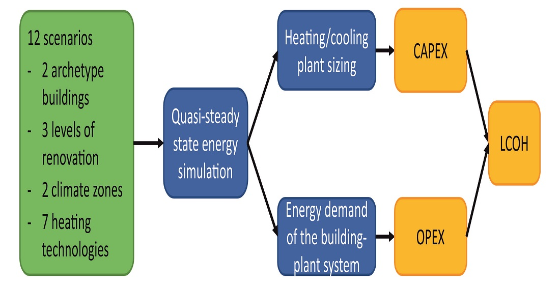
2. Methods
2.1. Benchmark Buildings and Thermal Needs Assessment
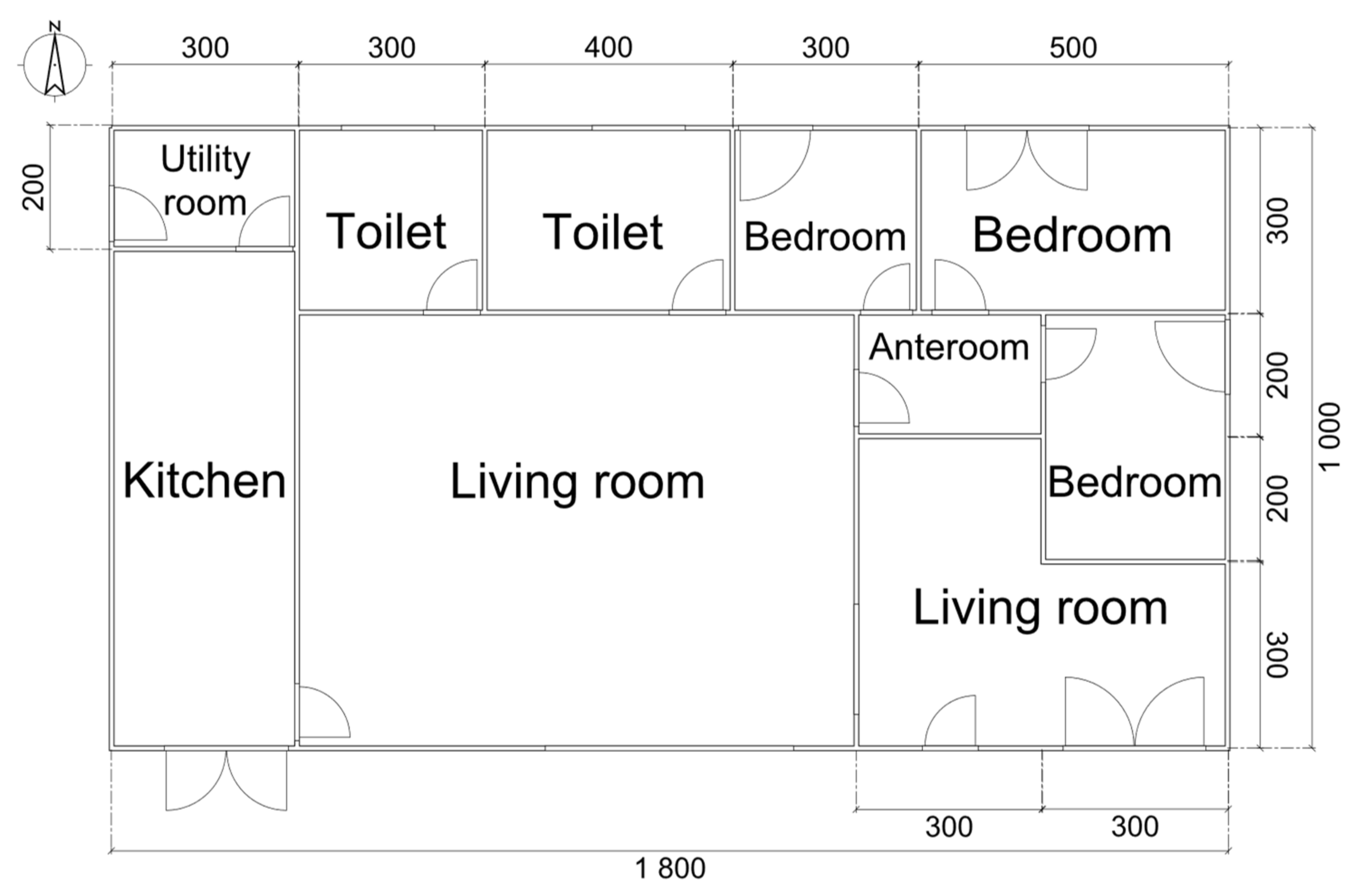
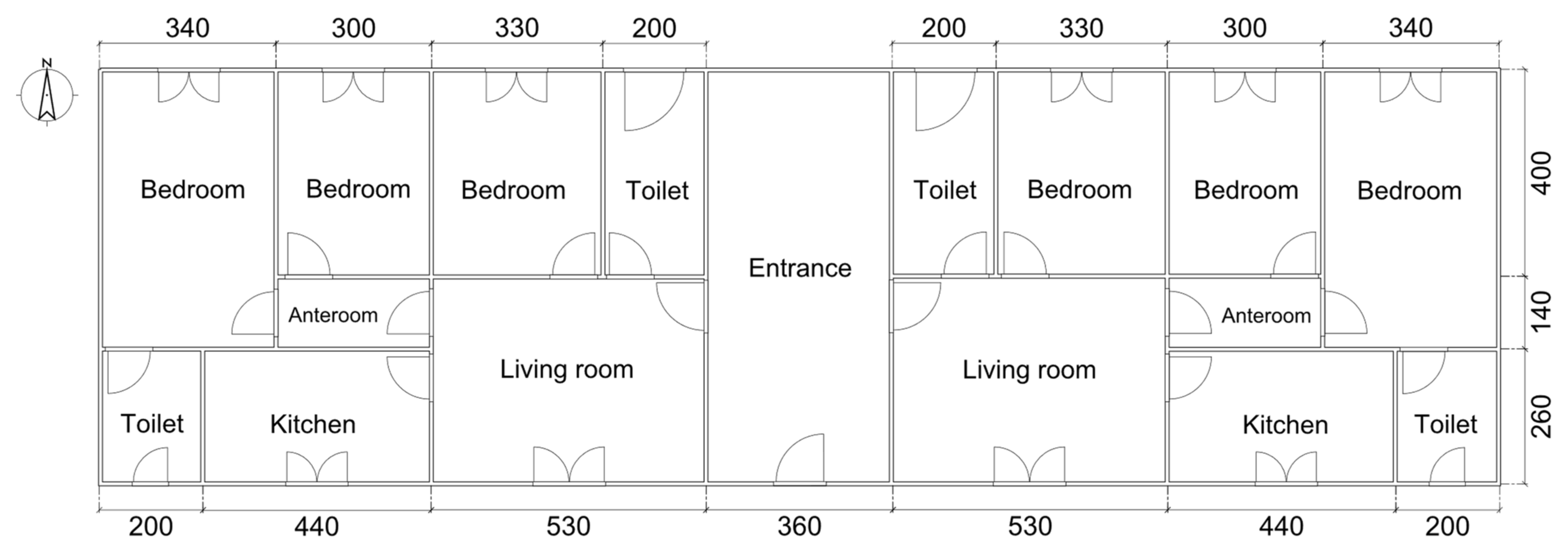
2.1.1. Choice of Representative Buildings and Locations
2.1.2. Assessment of Thermal Needs
2.2. Heating and Cooling Plant Sizing
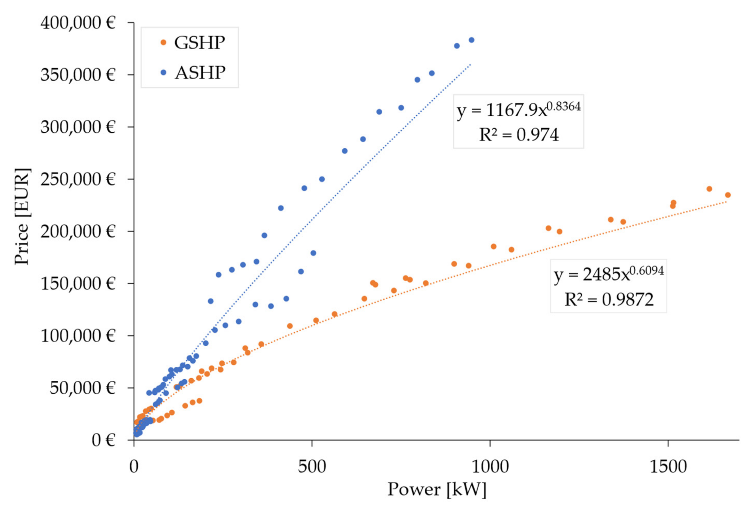
2.3. Estimation of the Initial Investment
2.4. Estimation of Operation and Maintenance Costs
2.4.1. Purchase of Fuel and Electricity
2.4.2. PV Systems and On-Site Exchange
2.4.3. Maintenance Costs
2.5. Levelized Cost of Heat (LCOH)
3. Results
3.1. Heating-Only Systems
3.2. Heating and Cooling Systems
- -
- The reversible heat pump models chosen in the heating-only analysis have a sufficient size to cover the cooling demand (except for scenario S11—the completely renovated apartment block in Turin—which requires an additional power of just 3 kW). However, including the cooling service makes it necessary to replace all radiators with fan coils (see Section 2.3).
- -
- For biomass and fossil fuel boilers, the cooling needs were deemed to be covered by a few mono-split air conditioners and, hence, a modest additional investment is needed.
3.3. Study Limitations
3.3.1. Uncertainty on Cost Items: Sensitivity Analysis
3.3.2. Temporary Factors Influencing LCOH
4. Discussion
- -
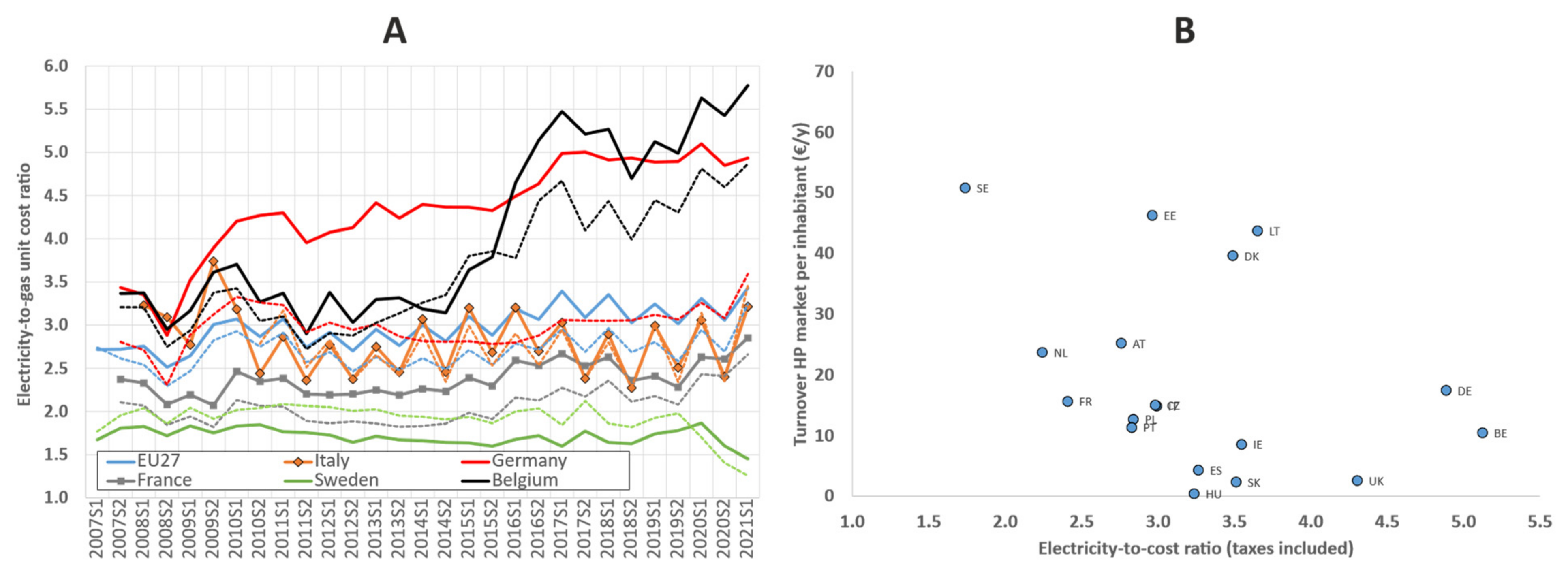
- A low electricity-to-gas cost ratio has a positive effect on the diffusion of heat pumps.
- -
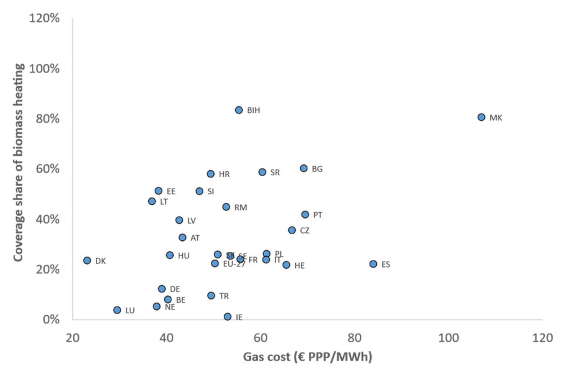
- A high gas cost (compared to purchasing power) has a positive effect on the diffusion of biomass heating.
5. Conclusions and Policy Implications
- -
- The Ecobonus incentive regime (and, a fortiori, with the Superbonus) makes renewable energy sources already the most economically viable solutions for space heating and DHW production.
- -
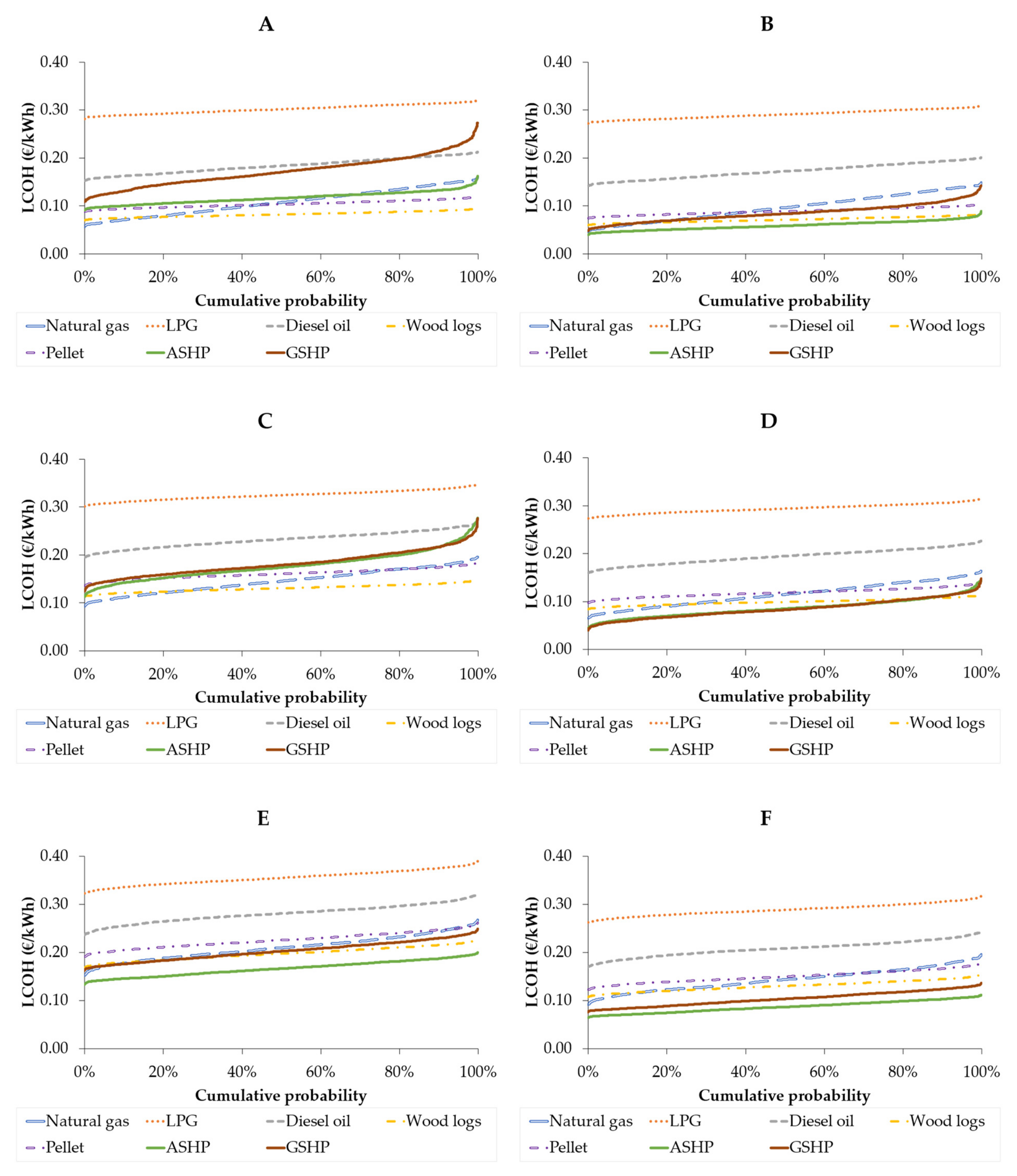
- Wood log boilers are generally the most affordable technology for space heating. Heat pumps (both air-source and ground-source) and pellet boilers follow in this ranking, with variable positions depending on the scenario.
- -
- The impact of the climate zone on LCOH values is generally modest. The only exception is represented by the GSHP systems installed in an apartment block. In this case, a colder climate (and, consequently, higher heating needs) leads to a relevant increase in the upfront costs of the BHE field.
- -
- Completely refurbished buildings are characterized by a higher LCOH value compared to partially refurbished buildings. This is because life-cycle costs are distributed based on lower heating demand.
- -
- In the climate zones of Piedmont, only completely renovated buildings have a relevant cooling demand.
- -
- The inclusion of space cooling demand makes heat pumps the most economically convenient solution to cover the thermal needs in the residential sector, with a slight advantage of the air-source type for detached houses and of the ground-source type for the blocks of apartments.
- -
- According to the sensitivity analysis carried out, the variability in input parameters of the economic analysis does not substantially alter the ranking of the economic viability of heating technologies.
- -
- The Ecobonus incentive is a sufficient stimulus to promote renewable heating, at least from the point of view of the LCOH.
- -
- The ratio between electricity and gas unit costs (EUR/MWh) is the critical parameter that drives the diffusion of heat pumps.
- -
- The unit cost of gas (normalized to the purchasing power of the country) is a good predictor of the diffusion of biomass heating.
- -
- Based on the above-reported facts, displacing the taxation from electricity-to-gas and reducing the cost of electricity (e.g., promoting self-production from PV such as in energy communities) can provide a further boost to the growth of heat pump installations.
Supplementary Materials
Author Contributions
Funding
Institutional Review Board Statement
Informed Consent Statement
Data Availability Statement
Acknowledgments
Conflicts of Interest
References
- European Commission European Green Deal: Commission Proposes Transformation of EU Economy and Society to Meet Climate Ambitions. Available online: https://bit.ly/36u98ch (accessed on 13 September 2021).
- European Commission EU Emissions Trading System (EU ETS). Available online: https://ec.europa.eu/clima/policies/ets_en (accessed on 1 October 2021).
- European Commission Carbon Border Adjustment Mechanism: Questions and Answers. Available online: https://bit.ly/3F7fJpE (accessed on 1 October 2021).
- European Commission Renewable Energy Directive 2018/2001/EU Known as RED2. Available online: https://bit.ly/RED2directive (accessed on 4 October 2021).
- Shen, W.; Chen, X.; Qiu, J.; Hayward, J.A.; Sayeef, S.; Osman, P.; Meng, K.; Dong, Z.Y. A Comprehensive Review of Variable Renewable Energy Levelized Cost of Electricity. Renew. Sustain. Energy Rev. 2020, 133, 110301. [Google Scholar] [CrossRef]
- Moseley, P.T.; Garche, J. Electrochemical Energy Storage for Renewable Sources and Grid Balancing; Elsevier: Amsterdam, The Netherlands, 2015; ISBN 978-0-444-62616-5. [Google Scholar]
- Roser, M. Why Did Renewables Become So Cheap So Fast? Available online: https://bit.ly/3In3Ex0 (accessed on 16 September 2021).
- Timilsina, G.R. Are Renewable Energy Technologies Cost Competitive for Electricity Generation? Renew. Energy 2021, 180, 658–672. [Google Scholar] [CrossRef]
- Lafond, F.; Bailey, A.G.; Bakker, J.D.; Rebois, D.; Zadourian, R.; McSharry, P.; Farmer, J.D. How Well Do Experience Curves Predict Technological Progress? A Method for Making Distributional Forecasts. Technol. Forecast. Soc. Change 2018, 128, 104–117. [Google Scholar] [CrossRef] [Green Version]
- Cui, Y.; Zhu, J.; Twaha, S.; Chu, J.; Bai, H.; Huang, K.; Chen, X.; Zoras, S.; Soleimani, Z. Techno-Economic Assessment of the Horizontal Geothermal Heat Pump Systems: A Comprehensive Review. Energy Convers. Manag. 2019, 191, 208–236. [Google Scholar] [CrossRef]
- Doračić, B.; Novosel, T.; Pukšec, T.; Duić, N. Evaluation of Excess Heat Utilization in District Heating Systems by Implementing Levelized Cost of Excess Heat. Energies 2018, 11, 575. [Google Scholar] [CrossRef] [Green Version]
- Doračić, B.; Pukšec, T.; Schneider, D.R.; Duić, N. The Effect of Different Parameters of the Excess Heat Source on the Levelized Cost of Excess Heat. Energy 2020, 201, 117686. [Google Scholar] [CrossRef]
- Li, H.; Song, J.; Sun, Q.; Wallin, F.; Zhang, Q. A Dynamic Price Model Based on Levelized Cost for District Heating. Energy Ecol. Environ. 2019, 4, 15–25. [Google Scholar] [CrossRef] [Green Version]
- Vivian, J.; Emmi, G.; Zarrella, A.; Jobard, X.; Pietruschka, D.; De Carli, M. Evaluating the Cost of Heat for End Users in Ultra Low Temperature District Heating Networks with Booster Heat Pumps. Energy 2018, 153, 788–800. [Google Scholar] [CrossRef]
- Wang, Z. Heat Pumps with District Heating for the UK’s Domestic Heating: Individual versus District Level. Energy Procedia 2018, 149, 354–362. [Google Scholar] [CrossRef]
- Renaldi, R.; Hall, R.; Jamasb, T.; Roskilly, A.P. Experience Rates of Low-Carbon Domestic Heating Technologies in the United Kingdom. Energy Policy 2021, 156, 112387. [Google Scholar] [CrossRef]
- Connor, P.M.; Xie, L.; Lowes, R.; Britton, J.; Richardson, T. The Development of Renewable Heating Policy in the United Kingdom. Renew. Energy 2015, 75, 733–744. [Google Scholar] [CrossRef]
- Fitó, J.; Dimri, N.; Ramousse, J. Competitiveness of Renewable Energies for Heat Production in Individual Housing: A Multicriteria Assessment in a Low-Carbon Energy Market. Energy Build. 2021, 242, 110971. [Google Scholar] [CrossRef]
- Atalla, T.; Gualdi, S.; Lanza, A. A Global Degree Days Database for Energy-Related Applications. Energy 2018, 143, 1048–1055. [Google Scholar] [CrossRef] [Green Version]
- Bettgenhäuser, K.; Offermann, M.; Boermans, T.; Bosquet, M.; Grözinger, J.; von Manteuffel, B.; Surmeli, N. An Analysis of the Technology’s Potential in the Building Sector of Austria, Belgium, Germany, Spain, France, Italy, Sweden and the United Kingdom. Available online: https://bit.ly/3pNv3BL (accessed on 8 March 2022).
- Eurostat Database—Energy. Available online: https://bit.ly/3klkvr3 (accessed on 17 September 2021).
- MISE Integrated National Energy and Climate Plan. Available online: https://bit.ly/NECP_IT (accessed on 20 September 2021).
- Casasso, A.; Capodaglio, P.; Simonetto, F.; Sethi, R. Environmental and Economic Benefits from the Phase-out of Residential Oil Heating: A Study from the Aosta Valley Region (Italy). Sustainability 2019, 11, 3633. [Google Scholar] [CrossRef] [Green Version]
- Sternberg, A.; Bardow, A. Power-to-What?—Environmental Assessment of Energy Storage Systems. Energy Environ. Sci. 2015, 8, 389–400. [Google Scholar]
- Casasso, A.; Tosco, T.; Bianco, C.; Bucci, A.; Sethi, R. How Can We Make Pump and Treat Systems More Energetically Sustainable? Water 2019, 12, 67. [Google Scholar] [CrossRef] [Green Version]
- Filippini, M.; Hunt, L.C.; Zorić, J. Impact of Energy Policy Instruments on the Estimated Level of Underlying Energy Efficiency in the EU Residential Sector. Energy Policy 2014, 69, 73–81. [Google Scholar] [CrossRef] [Green Version]
- Koengkan, M.; Fuinhas, J.A.; Osmani, F.; Kazemzadeh, E.; Auza, A.; Alavijeh, N.K.; Teixeira, M. Do Financial and Fiscal Incentive Policies Increase the Energy Efficiency Ratings in Residential Properties? A Piece of Empirical Evidence from Portugal. Energy 2022, 241, 122895. [Google Scholar] [CrossRef]
- Fuinhas, J.A.; Koengkan, M.; Silva, N.; Kazemzadeh, E.; Auza, A.; Santiago, R.; Teixeira, M.; Osmani, F. The Impact of Energy Policies on the Energy Efficiency Performance of Residential Properties in Portugal. Energies 2022, 15, 802. [Google Scholar] [CrossRef]
- Ballarini, I.; Pichierri, S.; Corrado, V. Tracking the Energy Refurbishment Processes in Residential Building Stocks. The Pilot Case of Piedmont Region. Energy Procedia 2015, 78, 1051–1056. [Google Scholar] [CrossRef] [Green Version]
- TABULA. EPISCOPE Joint EPISCOPE and TABULA Website. Available online: https://episcope.eu/welcome/ (accessed on 3 November 2021).
- Corrado, V.; Ballarini, I.; Corgnati, S.P. National Scientific Report on the TABULA Activities in Italy. Available online: http://bit.ly/TABULA_IT (accessed on 10 January 2020).
- Ballarini, I.; Corgnati, S.P.; Corrado, V. Use of Reference Buildings to Assess the Energy Saving Potentials of the Residential Building Stock: The Experience of TABULA Project. Energy Policy 2014, 68, 273–284. [Google Scholar] [CrossRef]
- MISE Requisiti Tecnici per l’accesso Alle Detrazioni Fiscali Per La Riqualificazione Energetica Degli Edifici—Cd. Ecobonus. (Technical Requirements for the Eligibility to Tax Deductions for Building Energy Refurbishment). Available online: https://bit.ly/DM20200806 (accessed on 3 November 2021).
- Repubblica Italiana DPR 412/1993—Regolamento Recante Norme Per La Progettazione, l’installazione, l’esercizio e La Manutenzione Degli Impianti Termici Degli Edifici Ai Fini Del Contenimento Dei Consumi Di Energia, in Attuazione Dell’art. 4, Comma 4, Della Legge 9 Gennaio 1991, n. 10. (Regulation for Designing, Installation, Operation and Maintenance of HVAC Systems). Available online: https://bit.ly/DPR41293 (accessed on 3 November 2021).
- TEP Software ANIT. Available online: https://www.anit.it/software-anit/ (accessed on 29 March 2021).
- UNI UNI/TS 11300 Standard Series. Available online: https://www.cti2000.eu/la-uni-ts-11300/ (accessed on 24 January 2022).
- ISO. ISO 13790:2008. Energy Performance of Buildings—Calculation of Energy Use for Space Heating and Cooling. Available online: https://www.iso.org/standard/41974.html (accessed on 16 March 2022).
- UNI UNI 10349:2016 Standard Series. Available online: https://bit.ly/3HSwyoD (accessed on 8 March 2022).
- ISTAT. I Consumi Energetici Delle Famiglie (Energetic Consumption of Italian Families, Divided by Region). Available online: https://www.istat.it/it/archivio/142173 (accessed on 17 September 2018).
- BLOCON EED—Earth Energy Designer. Version 4.20. Available online: https://buildingphysics.com/eed-2/ (accessed on 8 July 2021).
- Eskilson, P. Thermal Analysis of Heat Extraction Boreholes. Available online: http://bit.ly/2JCl6Be (accessed on 8 July 2021).
- Dalla Santa, G.; Galgaro, A.; Sassi, R.; Cultrera, M.; Scotton, P.; Mueller, J.; Bertermann, D.; Mendrinos, D.; Pasquali, R.; Perego, R.; et al. An Updated Ground Thermal Properties Database for GSHP Applications. Geothermics 2020, 85, 101758. [Google Scholar] [CrossRef]
- Bartolini, N.; Casasso, A.; Bianco, C.; Sethi, R. Environmental and Economic Impact of the Antifreeze Agents in Geothermal Heat Exchangers. Energies 2020, 13, 5653. [Google Scholar] [CrossRef]
- Repubblica Italiana D.Lgs. 28/2011—Attuazione Della Direttiva 2009/28/CE Sulla Promozione Dell’uso Dell’energia Da Fonti Rinnovabili, (Legislative Decree 28/2011 on the Promotion of Renewable Energy Sources, Applying the EC Directive 2009/28/EC). Available online: https://bit.ly/DLgs28_2011 (accessed on 4 January 2019).
- FERROLI. Price List. Available online: https://bit.ly/3Il4KJQ (accessed on 15 July 2021).
- FONDERIE SIME. Price List. Available online: https://bit.ly/3qfHTZT (accessed on 16 July 2021).
- MESCOLI. Price List. Available online: https://bit.ly/3we63ru (accessed on 3 September 2021).
- BOSCH. Price List. Available online: https://bit.ly/3wg8N7N (accessed on 2 September 2021).
- VAILLANT. Price List. Available online: https://bit.ly/3KRkoy5 (accessed on 10 September 2021).
- VIESSMANN. Price List. Available online: https://bit.ly/3KXDnr3 (accessed on 30 August 2021).
- Doseva, N.; Chakyrova, D. Life Cycle Cost Analysis of Different Residential Heat Pump Systems. E3S Web Conf. 2020, 207, 01014. [Google Scholar] [CrossRef]
- Vering, C.; Maier, L.; Breuer, K.; Krützfeldt, H.; Streblow, R.; Müller, D. Evaluating Heat Pump System Design Methods towards a Sustainable Heat Supply in Residential Buildings. Appl. Energy 2022, 308, 118204. [Google Scholar] [CrossRef]
- Regione Piemonte Prezzario delle Opere Pubbliche della Regione Piemonte (Price List of Public Works in the Piedmont Region). Available online: https://bit.ly/3o5aDCI (accessed on 31 March 2021).
- AERMEC. Italian Price List. Available online: https://bit.ly/3COeVWb (accessed on 1 September 2021).
- DAIKIN. Price List. Available online: https://bit.ly/3JrK7Ny (accessed on 4 September 2021).
- Blum, P.; Campillo, G.; Kölbel, T. Techno-Economic and Spatial Analysis of Vertical Ground Source Heat Pump Systems in Germany. Energy 2011, 36, 3002–3011. [Google Scholar] [CrossRef]
- BRGM. Action d’accompagnement Pour Le Développement de La Chaleur Géothermale. Convention ADEME-BRGM 2011—Synthèse. Rapport Final [Action for the Development of Geothermal Heat. Final Report]. Available online: http://infoterre.brgm.fr/rapports/RP-60843-FR.pdf (accessed on 25 February 2021).
- CCIAA. Torino Turin Chamber of Commerce—Biweekly Update on Fuel Prices. Available online: https://www.to.camcom.it/listino-quindicinale (accessed on 25 February 2021).
- GME. Italian Energy Market Manager (GME) Website—Sale Market Price. Available online: https://www.mercatoelettrico.org/it/ (accessed on 25 February 2021).
- CLIVET. CLIVET Manufacturer Website. Available online: https://www.clivet.com/ (accessed on 7 May 2021).
- GSE Italian Energy Service Manager (GSE)—Explanation of the on-Site Exchange Mechanism. Available online: https://www.gse.it/servizi-per-te/fotovoltaico/scambio-sul-posto (accessed on 5 May 2021).
- Hansen, K. Decision-Making Based on Energy Costs: Comparing Levelized Cost of Energy and Energy System Costs. Energy Strategy Rev. 2019, 24, 68–82. [Google Scholar] [CrossRef]
- Eicher, S.; Hildbrand, C.; Kleijer, A.; Bony, J.; Bunea, M.; Citherlet, S. Life Cycle Impact Assessment of a Solar Assisted Heat Pump for Domestic Hot Water Production and Space Heating. Energy Procedia 2014, 48, 813–818. [Google Scholar] [CrossRef] [Green Version]
- Latorre-Biel, J.-I.; Jimémez, E.; García, J.L.; Martínez, E.; Jiménez, E.; Blanco, J. Replacement of Electric Resistive Space Heating by an Air-Source Heat Pump in a Residential Application. Environmental Amortization. Build. Environ. 2018, 141, 193–205. [Google Scholar] [CrossRef]
- Pike, C.; Whitney, E. Heat Pump Technology: An Alaska Case Study. J. Renew. Sustain. Energy 2017, 9, 061706. [Google Scholar] [CrossRef]
- Ma, Z.J.; Thomas, S. Reliability and Maintainability in Photovoltaic Inverter Design. In Proceedings of the 2011 Annual Reliability and Maintainability Symposium, Lake Buena Vista, FL, USA, 24–27 January 2011; pp. 1–5. [Google Scholar] [CrossRef]
- Abdul-Ganiyu, S.; Quansah, D.A.; Ramde, E.W.; Seidu, R.; Adaramola, M.S. Techno-Economic Analysis of Solar Photovoltaic (PV) and Solar Photovoltaic Thermal (PVT) Systems Using Exergy Analysis. Sustain. Energy Technol. Assess. 2021, 47, 101520. [Google Scholar] [CrossRef]
- Nitkiewicz, A.; Sekret, R. Comparison of LCA Results of Low Temperature Heat Plant Using Electric Heat Pump, Absorption Heat Pump and Gas-Fired Boiler. Energy Convers. Manag. 2014, 87, 647–652. [Google Scholar] [CrossRef]
- Casasso, A.; Puleo, M.; Panepinto, D.; Zanetti, M. Economic Viability and Greenhouse Gas (GHG) Budget of the Biomethane Retrofit of Manure-Operated Biogas Plants: A Case Study from Piedmont, Italy. Sustainability 2021, 13, 7979. [Google Scholar] [CrossRef]
- Mohammadpourkarbasi, H.; Sharples, S. Appraising the Life Cycle Costs of Heating Alternatives for an Affordable Low Carbon Retirement Development. Sustain. Energy Technol. Assess. 2022, 49, 101693. [Google Scholar] [CrossRef]
- Poponi, D.; Basosi, R.; Kurdgelashvili, L. Subsidisation Cost Analysis of Renewable Energy Deployment: A Case Study on the Italian Feed-in Tariff Programme for Photovoltaics. Energy Policy 2021, 154, 112297. [Google Scholar] [CrossRef]
- Reber, T.J.; Beckers, K.F.; Tester, J.W. The Transformative Potential of Geothermal Heating in the U.S. Energy Market: A Regional Study of New York and Pennsylvania. Energy Policy 2014, 70, 30–44. [Google Scholar] [CrossRef]
- AFPG. Etude Techno-Économique de La Géothermie de Surface (Techno-Economic Study of Shallow Geothermal Energy). Available online: https://bit.ly/3G80L2G (accessed on 1 December 2021).
- Luo, J.; Zhang, Y.; Rohn, J. Analysis of Thermal Performance and Drilling Costs of Borehole Heat Exchanger (BHE) in a River Deposited Area. Renew. Energy 2020, 151, 392–402. [Google Scholar] [CrossRef]
- IEA. Cumulative Capacity and Capital Cost Learning Curve for Vapour Compression Applications in the Sustainable Development Scenario, 2019–2070. Available online: https://bit.ly/3D86rrf (accessed on 9 September 2021).
- Köhler, B.; Stobbe, M.; Garzia, F. EU H2020 Project CRAVEzero. Deliverable D.4.1. Guideline II: NZEB Technologies: Report on Cost Reduction Potentials for Technical NZEB Solution Sets. Available online: https://bit.ly/3G0BUi2 (accessed on 9 September 2021).
- European Commission, Joint Research Centre. Li-Ion Batteries for Mobility and Stationary Storage Applications: Scenarios for Costs and Market Growth; Publications Office: Luxembourg, 2018. [Google Scholar]
- IEA. What Is Behind Soaring Energy Prices and What Happens Next? Available online: https://bit.ly/3ie70I5 (accessed on 16 March 2022).
- Trading Economics EU Natural Gas—2022 Data—2010–2021 Historical. Available online: https://bit.ly/3ibcKm7 (accessed on 16 March 2022).
- Martinopoulos, G.; Papakostas, K.T.; Papadopoulos, A.M. A Comparative Review of Heating Systems in EU Countries, Based on Efficiency and Fuel Cost. Renew. Sustain. Energy Rev. 2018, 90, 687–699. [Google Scholar] [CrossRef]
- Novelli, A.; D’Alonzo, V.; Pezzutto, S.; Poggio, R.A.E.; Casasso, A.; Zambelli, P. A Spatially-Explicit Economic and Financial Assessment of Closed-Loop Ground-Source Geothermal Heat Pumps: A Case Study for the Residential Buildings of Valle d’Aosta Region. Sustainability 2021, 13, 12516. [Google Scholar] [CrossRef]
- Bertelsen, N.; Vad Mathiesen, B. EU-28 Residential Heat Supply and Consumption: Historical Development and Status. Energies 2020, 13, 1894. [Google Scholar] [CrossRef]
- POLIMI. Smart Building Report 2020. Energy Efficiency and Digital Technologies to Improve the Building Sector (Original Title in Italian). Available online: https://bit.ly/35Xr3YT (accessed on 14 March 2022).
- Barnes, J.; Bhagavathy, S.M. The Economics of Heat Pumps and the (Un)Intended Consequences of Government Policy. Energy Policy 2020, 138, 111198. [Google Scholar] [CrossRef]
- Boldrin, G. Transfer of Credit and Discount on Invoice for Tax Deductions: Analysis and Evolution (Original Title in Italian). Master’s Thesis, University of Venezia “Ca’ Foscari”, Venezia, Italy. Available online: https://bit.ly/3CGuD5o (accessed on 14 March 2022).
- EHPA. European Heat Pump Market and Statistic Report 2020 & Stats Tool. Available online: http://www.stats.ehpa.org/hp_sales/country_cards/ (accessed on 15 March 2022).
- Eurostat. Final Energy Consumption in Households by Type of Fuel. Available online: https://ec.europa.eu/eurostat/databrowser/view/ten00125/default/table?lang=en (accessed on 15 March 2022).
- Bioenergy Europe Bioenergy Europe Statistical Report. 2020. Available online: https://bit.ly/36kZPuR (accessed on 15 March 2022).
- Sarigiannis, D.A.; Karakitsios, S.P.; Kermenidou, M.V. Health Impact and Monetary Cost of Exposure to Particulate Matter Emitted from Biomass Burning in Large Cities. Sci. Total Environ. 2015, 524–525, 319–330. [Google Scholar] [CrossRef]
- Verkerk, P.J.; Fitzgerald, J.B.; Datta, P.; Dees, M.; Hengeveld, G.M.; Lindner, M.; Zudin, S. Spatial Distribution of the Potential Forest Biomass Availability in Europe. For. Ecosyst. 2019, 6, 5. [Google Scholar] [CrossRef]
- Malico, I.; Nepomuceno Pereira, R.; Gonçalves, A.C.; Sousa, A.M.O. Current Status and Future Perspectives for Energy Production from Solid Biomass in the European Industry. Renew. Sustain. Energy Rev. 2019, 112, 960–977. [Google Scholar] [CrossRef]
- Ruiz, P.; Nijs, W.; Tarvydas, D.; Sgobbi, A.; Zucker, A.; Pilli, R.; Jonsson, R.; Camia, A.; Thiel, C.; Hoyer-Klick, C.; et al. ENSPRESO—An Open, EU-28 Wide, Transparent and Coherent Database of Wind, Solar and Biomass Energy Potentials. Energy Strategy Rev. 2019, 26, 100379. [Google Scholar] [CrossRef]


| Component | Original U-Value | Climatic Zone | Required U-Value |
|---|---|---|---|
| Upper roof | 1.65 | E | 0.20 |
| F | 0.19 | ||
| Lower floor | 1.30 | E | 0.25 |
| F | 0.23 | ||
| Perimetral walls | 1.26 | E | 0.23 |
| F | 0.22 | ||
| Windows | 2.8 | E | 1.30 |
| F | 1.00 |
| Model Building | Location | Original Building | Partial Renovation | Complete Renovation | ||||||
|---|---|---|---|---|---|---|---|---|---|---|
| # | Heating | Cooling | # | Heating | Cooling | # | Heating | Cooling | ||
| Single detached house | Turin | S01 | 29.05 (186.22) | 0.87 (5.58) | S05 | 26.42 (169.36) | 0.83 (5.32) | S09 | 7.85 (50.32) | 2.34 (15.00) |
| Oulx | S02 | 42.61 (273.14) | 0.00 (0.00) | S06 | 38.62 (247.56) | 0.00 (0.00) | S10 | 10.96 (70.26) | 0.51 (3.27) | |
| Apartment block | Turin | S03 | 115.37 (123.52) | 12.32 (13.19) | S07 | 101.25 (108.40) | 12.53 (13.42) | S11 | 17.03 (18.23) | 24.81 (26.56) |
| Oulx | S04 | 172.89 (185.11) | 0.68 (0.73) | S08 | 152.35 (163.12) | 0.89 (0.95) | S12 | 26.91 (28.81) | 13.14 (14.07) | |
| Typology | Cost (<35 kW) | Cost (65–70 kW) |
|---|---|---|
| Gas boiler | EUR 6860 | EUR 9255 |
| LPG boiler | EUR 6860 | EUR 9255 |
| Oil boiler | EUR 7175 | EUR 9255 |
| Wood logs boiler | EUR 7015 | EUR 9270 |
| Pellet boiler | EUR 7015 | EUR 9270 |
| Energy Source | Value | Unit | Validity Range | Reference | ||
|---|---|---|---|---|---|---|
| Min | Max | Unit | ||||
| Natural gas for household consumers | 148 | EUR/MWh | - | 6 | MWh | [21] |
| 93 | EUR/MWh | 6 | 56 | MWh | ||
| 74 | EUR/MWh | 56 | - | MWh | ||
| Diesel oil | 1.34 | EUR/l | - | - | - | [58] |
| 135 | EUR/MWh | - | - | - | ||
| LPG (tank on loan) | 1.53 | EUR/l | - | - | - | [58] |
| 230 | EUR/MWh | - | - | - | ||
| Wood logs | 150 | EUR/ton | - | - | - | [58] |
| 41 | EUR/MWh | - | - | - | ||
| Pellet (15 kg bags) | 290 | EUR/ton | - | - | - | [58] |
| 58 | EUR/MWh | - | - | - | ||
| Electricity for household consumers | 252 | EUR/MWh | 1 | 2.5 | MWh | [21] |
| 234 | EUR/MWh | 2.5 | 5 | MWh | ||
| 232 | EUR/MWh | 5 | 15 | MWh | ||
| 225 | EUR/MWh | 15 | - | MWh | ||
| National price of electricity with on-site power exchange | 67 | EUR/MWh | - | - | - | [59] |
| Intervention | Capacity Range (kW) | Cost (EUR, VAT Excl.) |
|---|---|---|
| Preventive maintenance for natural gas boilers | <35 kW | 80 |
| 35–60 kW | 120 | |
| 60–100 kW | 150 | |
| Preventive maintenance for oil boilers | <35 kW | 110 |
| 35–60 kW | 130 | |
| 60–100 kW | 180 | |
| Preventive maintenance for wood boilers | <35 kW | 150 |
| 35–100 kW | 250 | |
| Preventive maintenance for pellet boilers | <35 kW | 110 |
| 35–100 kW | 220 | |
| Combustion analysis | <35 kW | 40 |
| 35–100 kW | 50 | |
| Descaling of exchangers and boilers | <35 kW | 50 |
| Heat pumps and chillers | <35 kW | 150 |
| 35–100 kW | 250 |
| Building | Renovation | Location (Scenario) | NG | LPG | OIL | WL | PEL | AS | GSlc | GSmc | GShc |
|---|---|---|---|---|---|---|---|---|---|---|---|
| Single detached house | Partial | Turin (S05) | 128.5 | 290.7 | 179.6 | 70.3 | 89.6 | 78.8 | 83.8 | 80.7 | 78.7 |
| −8% | −4% | −6% | −14% | −14% | −47% | −48% | −48% | −48% | |||
| Oulx (S06) | 127.2 | 296.6 | 180.2 | 62.1 | 84.1 | 72.6 | 84.5 | 75.4 | 73.2 | ||
| −6% | −2% | −4% | −11% | −11% | −46% | −47% | −50% | −49% | |||
| Complete | Turin (S09) | 142.2 | 292.6 | 198.6 | 97.7 | 118.7 | 96.2 | 114.6 | 111.3 | 109.4 | |
| −18% | −9% | −16% | −24% | −26% | −48% | −50% | −50% | −50% | |||
| Oulx (S10) | 130.7 | 278.3 | 183.5 | 83.8 | 103.3 | 58.5 | 82.2 | 76.2 | 74.0 | ||
| −15% | −8% | −13% | −22% | −23% | −44% | −49% | −49% | −48% | |||
| Apartment block | Partial | Turin (S07) | 92.5 | 273.9 | 163.9 | 55.7 | 72.1 | 81.9 | 71.7 | 64.4 | 61.3 |
| −4% | −1% | −2% | −5% | −4% | −38% | −49% | −49% | −49% | |||
| Oulx (S08) | 91.2 | 273.3 | 162.7 | 53.6 | 70.3 | 78.7 | 101.5 | 80.6 | 73.2 | ||
| −3% | −1% | −1% | −3% | −3% | −31% | −45% | −43% | −41% | |||
| Complete | Turin (S11) | 110.9 | 252.5 | 157.8 | 60.3 | 77.2 | 65.4 | 66.6 | 63.5 | 61.6 | |
| −8% | −4% | −7% | −14% | −15% | −48% | −49% | −49% | −49% | |||
| Oulx (S12) | 109.8 | 252.9 | 155.9 | 57.1 | 73.7 | 62.0 | 71.1 | 66.6 | 64.4 | ||
| −6% | −3% | −5% | −11% | −12% | −47% | −49% | −48% | −48% |
| Building | Location | Quantity | NG | LPG | OIL | WL | PEL | AS | GSlc | GSmc | GShc |
|---|---|---|---|---|---|---|---|---|---|---|---|
| Single detached house | Turin (S09) | LCOH | 171.3 | 293.4 | 217 | 134.4 | 155 | 93.1 | 110.8 | 108.4 | 107.1 |
| Δh&c | 20% | 0% | 9% | 38% | 31% | −3% | −3% | −3% | −2% | ||
| Oulx (S10) | LCOH | 176.2 | 318.4 | 227.1 | 130.7 | 152.5 | 88.5 | 108.6 | 102.9 | 100.8 | |
| Δh&c | 35% | 14% | 24% | 56% | 48% | 51% | 32% | 35% | 36% | ||
| Apartment block | Turin (S11) | LCOH | 106.8 | 184.8 | 132 | 78.1 | 89.8 | 56 | 52.6 | 48.7 | 47.1 |
| Δh&c | −4% | −27% | −16% | 30% | 16% | −14% | −21% | −23% | −24% | ||
| Oulx (S12) | LCOH | 114.8 | 223.8 | 149.4 | 74.2 | 88.7 | 60.6 | 54.5 | 52.4 | 50.7 | |
| Δh&c | 5% | −12% | −4% | 30% | 20% | −2% | −23% | −21% | −21% |
| Variable | Unit | Min | Max | Notes |
|---|---|---|---|---|
| Electricity price for household consumers | EUR/MWh | 49 | 334 | 1000–2500 kWh |
| EUR/MWh | 98 | 301 | 2500–5000 kWh | |
| EUR/MWh | 95 | 280 | 5000–15,000 kWh | |
| EUR/MWh | 95 | 313 | >15,000 kWh | |
| National price on power exchange | EUR/MWh | 0 | 163 | - |
| Natural gas price for household consumers | EUR/MWh | 31 | 160 | <20 GJ |
| EUR/MWh | 28 | 107 | 20–200 GJ | |
| EUR/MWh | 27 | 104 | >200 GJ | |
| Diesel oil | EUR/l | 1.06 | 1.51 | - |
| LPG | EUR/l | 1.45 | 1.62 | - |
| Wood | EUR/kg | 0.13 | 0.18 | - |
| Pellet | EUR/kg | 0.24 | 0.34 | - |
| BHEs drilling and setting cost | EUR/m | 40 | 75 | - |
| ASHP cost | Variation | −9% | +9% | - |
| GSHP cost | Variation | −9% | +9% | - |
| Batteries cost | Variation | −12% | +12% | - |
| Discount rate | % | 2% | 6% | - |
Publisher’s Note: MDPI stays neutral with regard to jurisdictional claims in published maps and institutional affiliations. |
© 2022 by the authors. Licensee MDPI, Basel, Switzerland. This article is an open access article distributed under the terms and conditions of the Creative Commons Attribution (CC BY) license (https://creativecommons.org/licenses/by/4.0/).
Share and Cite
Ruffino, E.; Piga, B.; Casasso, A.; Sethi, R. Heat Pumps, Wood Biomass and Fossil Fuel Solutions in the Renovation of Buildings: A Techno-Economic Analysis Applied to Piedmont Region (NW Italy). Energies 2022, 15, 2375. https://0-doi-org.brum.beds.ac.uk/10.3390/en15072375
Ruffino E, Piga B, Casasso A, Sethi R. Heat Pumps, Wood Biomass and Fossil Fuel Solutions in the Renovation of Buildings: A Techno-Economic Analysis Applied to Piedmont Region (NW Italy). Energies. 2022; 15(7):2375. https://0-doi-org.brum.beds.ac.uk/10.3390/en15072375
Chicago/Turabian StyleRuffino, Edoardo, Bruno Piga, Alessandro Casasso, and Rajandrea Sethi. 2022. "Heat Pumps, Wood Biomass and Fossil Fuel Solutions in the Renovation of Buildings: A Techno-Economic Analysis Applied to Piedmont Region (NW Italy)" Energies 15, no. 7: 2375. https://0-doi-org.brum.beds.ac.uk/10.3390/en15072375