
Control of a Three-Phase Current Source Rectifier for H2 Storage Applications in AC Microgrids
by
 , and
, and
Quentin Combe
† ,
,
Alireza Abasian
†,
Serge Pierfederici
*,†,
Mathieu Weber
† and
Stéphane Dufour
† LEMTA, Université de Lorraine, 2 Avenue de la Foret de Haye, 54500 Vandoeuvre-les-Nancy, France
*
Author to whom correspondence should be addressed.
†
These authors contributed equally to this work.
Energies 2022, 15(7), 2436; https://0-doi-org.brum.beds.ac.uk/10.3390/en15072436
Submission received: 8 February 2022
/
Revised: 21 March 2022
/
Accepted: 23 March 2022
/
Published: 25 March 2022
(This article belongs to the Special Issue Volume II: Energy Management Systems for Optimal Operation of Electrical Micro/Nanogrids)
Abstract
:The share of electrical energy from renewable sources has increased considerably in recent years in an attempt to reduce greenhouse gas emissions. To mitigate the uncertainties of these sources and to balance energy production with consumption, an energy storage system (ESS) based on water electrolysis to produce hydrogen is studied. It can be applied to AC microgrids, where several renewable energy sources and several loads may be connected, which is the focus of the study. When excess electricity production is converted into hydrogen via water electrolysis, low DC voltages and high currents are applied, which needs specific power converters. The use of a three-phase, buck-type current source converter, in a single conversion stage, allows for an adjustable DC voltage to be obtained at the terminals of the electrolyzer from a three-phase AC microgrid. The voltage control is preferred to the current control in order to improve the durability of the system. The classical control of the buck-type rectifier is generally done using two loops that correspond only to the control of its output variables. The lack of control of the input variables may generate oscillations of the grid current. Our contribution in this article is to propose a new control for the buck-type rectifier that controls both the input and output variables of the converter to avoid these grid current oscillations, without the use of active damping methods. The suggested control method is based on an approach using the flatness properties of differential systems: it ensures the large-signal stability of the converter. The proposed control shows better results than the classical control, especially in oscillation mitigation and dynamic performances with respect to the rejection of disturbances caused by a load step.
1. Introduction
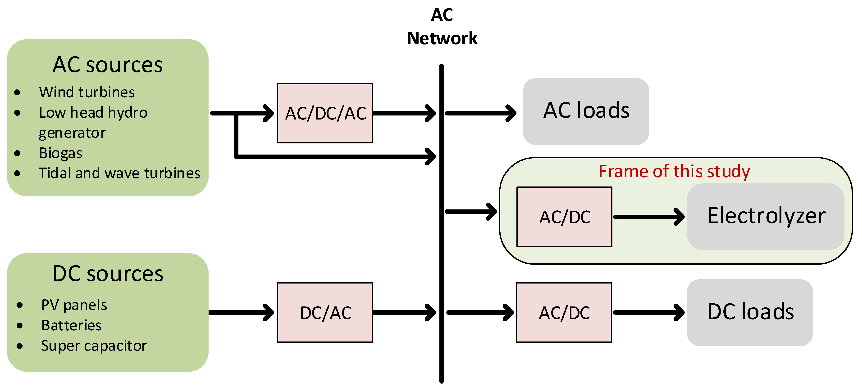
In recent years, the development of renewable energies has accelerated with the aim of reducing the share of electricity production that is carried out by means that emit high levels of greenhouse gases, such as gas-fired power stations or, even worse, those using coal [1,2]. In this study, we will consider the context of AC microgrids, in which there are several sources of renewable energy and several loads (Figure 1). The AC network has been used as the standard choice for energy transmission systems since the 19th century for its many advantages such as [3]:
- Power transmission over a long distance;
- AC voltage magnitude conversion.
The renewable energy sources are, by nature, intermittent and it is, therefore, difficult to balance energy production with consumption when the share of renewables in the energy mix is significant. To compensate for the intermittency of these sources and the fact that their production cannot be controlled, ESSs are a true solution [4]. Among the different types of ESSs, it is possible to highlight two categories: those using batteries [5] and those using hydrogen production by water electrolysis [6]. In the following, we will consider the case that consists of converting the excess electricity production into hydrogen by water electrolysis [7].
This solution allows for the maintenance of the grid frequency, even in the case of low power demand. Hydrogen production based on renewable energy or low-carbon power is called green hydrogen. It has significantly lower carbon emissions than grey hydrogen, which is produced by the steam-reforming of natural gas, which constitutes the bulk of the hydrogen market [8]. Green hydrogen appears to be an attractive energy vector to reduce the carbon footprint of the transportation sector and industrial processes. Unfortunately, due to the high cost of production, green hydrogen represents less than of total hydrogen production [9].
To convert the excess electricity production into hydrogen, it is necessary to use a converter connected to this AC microgrid to feed the electrolyzer. A state-of-the-art representation of the conversion structures is presented in [10]. Most topologies can be classified into four main categories, which are presented in Figure 2, among which three of them consider controlled converters.
Currently, thyristor-based solutions are the most widely used in industrial applications [11,12], especially in electrolysis, due to the necessity of high current generation to supply high-power electrolyzers. However, the use of thyristors implies the generation of reactive power, which dramatically reduces the power factor. In addition, the output current ripple is quite high, which leads to an increase in energy consumption [13,14].
The second category is a combination of the rectifier with a DC chopper. It avoids the use of passive filters as it can improve the power quality. It is important to combine new emerging DC-DC converters with power management strategies to improve the energy efficiency and the hydrogen flow rate [15].
The third category is the pulse-width modulation (PWM) current-source rectifiers (CSR). They appear as attractive topologies regarding the power quality and their dynamic behavior, even if they seem to be limited to medium-voltage applications to maintain good efficiency, which is in the scope of the application [16].
In this study, the CSR is used to interface the electrolyzer with the grid. To control an electrolyzer, two ways are possible: either impose the voltage or the current. Since the current control, in the case of a cell malfunction, leads to an increase of the electric potential at the cell terminals which may irreversibly damage the cell, the choice was made to use a rectifier that allows one to control the voltage at the electrolyzer terminals. It improves the durability of the systems, especially in the case of cell aging.
As the hydrogen production rate is directly linked to the current flowing through the electrolyzer, it is necessary to use a converter that provides high currents for (relatively) low voltages. Since the typical voltage of a cell is about 1.8 V, and as a classical stack contains 100 of these cells in series, the voltage is about 180 V, whereas the current is about 1000 A. To link the electrolyzer to a classical US grid AC network, the use of a three-phase buck is suggested here, since it is a suitable option for applications that require a lower DC output voltage than the AC mains. The topology has already attracted the attention for different applications such as wind energy conversion systems [17] and on-board electric vehicle chargers [18,19]. This topology is becoming more attractive for motor-drive applications. The classical topology is used in [20], while a novel one is presented in [21] to improve the reliability. Commutation methods in current source inverters (CSI) that use four-quadrant switches are presented in [22] to improve the efficiency compared to conventional CSI with series power diodes.
The classical topology of a buck-type rectifier is studied here because it is a fair compromise between good performance and a low number of semi-conductors to achieve the step-down function. In a single conversion stage, this converter allows one to adjust the output DC voltage, while ensuring a sinusoidal grid current in phase with the main phase voltage [23].
The classical control deals only with output variables of the converter at the price of grid current oscillations, which are undesirable for AC microgrids. The presence of oscillations inside the grid current is explained by the resonance of the filter excited by the harmonics generated by the switching of the transistors. These oscillations are traditionally reduced with damping methods [24]. The proposed synthesis naturally integrates the presence of the input filter and guarantees the stability of the system for all operating points.
The improvement of the control that is proposed here is a stategy based on the control of input and output variables at the same time, in order to directly control grid current oscillations without the need of damping methods. As the proposed control method is based on an approach using the flatness properties of differential systems, it also ensures the large-signal stability of the converter.
The paper is organized as follows: Section 2 describes the operation principle and the modeling of this converter; Section 3 details the proposed control to improve the converter performance; Section 4 deals with the sensibility analysis; and, finally, Section 5 and Section 6 display a simulation and experimental results to validate the proposed solution.
2. Operation Principle and Modelisation
2.1. Instantaneous Model
The topology is based on an unidirectional CSR with six transistors in series with six diodes to ensure a bidirectional voltage blocking capability. The harmonics injected by the buck rectifier into the microgrid are reduced by an input differential mode filter.
One of the advantages of this topology is the absence of a high start-up current and the naturally induced protection under legs short circuit [25]. Due to the presence of an inductance at the output, the current is approximately constant.
At each time, only one high-side SiH and one low-side SiL switch have to be turned on. If, simultaneously, more than one switch is conducting at the upper side or at the lower side, the state of their series diode will be defined by the sign of the phase-to-phase voltage associated with the two bridge legs. Due to voltage ripple and the fact that at each sector crossover, the line voltage is equal to zero, this can lead to the series diodes turning on simultaneously. This generates a distortion of the grid current [26].
A freewheeling diode, , is added: without any command on the switches, the DC output voltage is zero. This functionality could be performed by short-circuiting a leg, but at the price of higher switching losses (the pattern would contain a higher number of vectors), and higher conduction losses (the current would flow in a higher number of semiconductors) [27]. The freewheeling diode, , also ensures the continuity of the current inside the output inductance, . It is conducting when all switches are open. If the switches S1H and S2L (shown in Figure 3) are conducting, the output current, , flows from phase a and returns back into phase b.
In this case, the line-to-line voltage is applied to the output. The maximum output voltage of this converter is [27]:
where is the power factor and the grid nominal line voltage. To get the maximum achievable output voltage, the rectifier has to operate at a unity power factor; that is to say that grid current and phase voltage have to be in phase. In this case, the reactive power generated by the input filter is totally compensated.
To establish the time varying differential equations of the converter, the boolean switching variables SiH and SiL are considered with (1 value for a closed switch, 0 when open). They can be put in a vector form:
The equations of this converter can be written as follows (where the exponent T stands for the transpose):
As this model uses boolean switching variables, it requires the Space Vector Modulation (SVM) part to determine the dynamics of the converter. Unfortunately, adding this part makes the model more difficult to implement and leads to an increase of the computer simulation time; the characteristic time of the switches is far lower than the time constants of the other variables. This is why it is preferable to work with an average time model in which all variables are replaced by their average values computed over a switching period T.
2.2. Space Vector Modulation
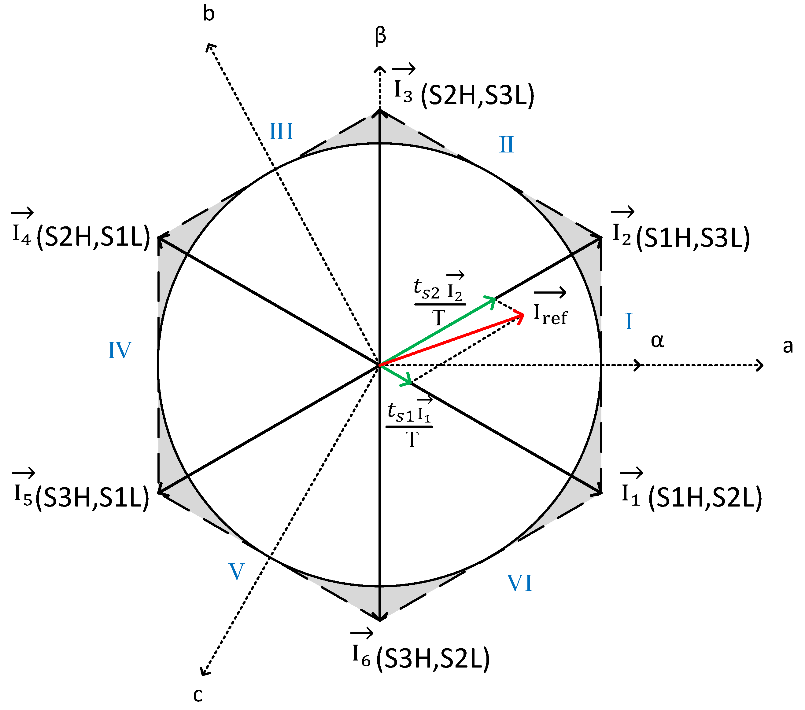
The SVM technique consists of controlling the reference vector in the frame in which the converter generates only six active current vectors, with each vector being a combination of different active switches. With six switches, and two states for each switch (open or closed), we have theoretical possibilities; however, due to the operating conditions stated above, there are six active vectors and four zero vectors. The zero-state vector will be performed here by the opening of all the switches, thanks to the freewheeling diode .
The importance of the modulation scheme has been studied in [28] and an overview has been presented in [29]. Since the study of the modulation scheme is not the scope of this article, the choice was made to use the six-sector Modified Full wave Symmetrical Modulation (MFSM) scheme (Figure 4) to facilitate its practical implementation into the FPGA. The change of sector is eased since the zero-state vector is used on both neighboring sectors. Next, the FPGA will generate the command for the drivers of the switches.
An SVM is decomposed in three steps:
- 1.
- Identify in which sector the reference vector is;
- 2.
- Compute the application times of adjacent vectors and the zero-state vector during a switching period T;
- 3.
- Choose the modulation sequence during a switching period.
The six vectors shown in Figure 5 correspond to an unique combination of the six switches. For example, the vector corresponds to the following combination:
If we directly use these vectors, we are in the full-wave command. To control the reference vector in phase and magnitude, a temporal aspect has to be added: this is the Pulse Width Modulation (PWM). To apply the reference vector, we build an average vector that results from the association of two adjacent vectors, , and one zero-state vector, , whose order of application depends on the selected pattern. In Figure 5, the area of application of the reference vector that corresponds to the circle inscribed inside the hexagon can be seen. Each active vector has a modulus equal to:
The maximum modulus for the reference vector is:
The modulation index, M, is defined by the ratio between the reference vector modulus and its maximum:
Its value is between 0 and 1.
2.3. Average Model
The source phase voltages are assumed to form a direct balanced system:
To get almost constant variables, Concordia and Park transformations are performed to move from an abc to a dq frame. The transformations of the variables X are done as follows:
The phase voltages are in the Park’s reference frame and .
Using (4a) and (9), the grid current equation becomes:
The instantaneous expression averaged during one switching period of the input current of the rectifier in frame can be obtained using:
This allows us to define:
The governing equation of the output current, , is:
Moreover, we can write:
Therefore, it is possible to write the equation as a power balance between the input and the output of the converter, where corresponds to the reference of active power consumed by the rectifier.
This leads to the following system of differential equations:
This formulation allows one to work with the reference vector , where its components and are the control variables of the active power and the reactive power consumed by the converter, respectively.
As the model only needs values for in a state-space model, its simulation is faster than the whole model with the SVM part.
3. Proposed Control for the Three-Phase Buck-Type Rectifier
3.1. The Principle of Flatness of Differential Systems
A non-linear system , composed of a state vector and an input vector , is considered as flat if, and only if, there exists a flat output vector y composed of m elements and the functions and , such that it is possible to write [30]:
where r and s are integers. When a system is flat, the dynamics of the state variables are described by the flat outputs and a finite number of their derivatives. Therefore, if the trajectory of the flat output is well controlled, the trajectory of the state and control variables are also well known, even during transient. The trajectory planning of the flat outputs allows one to generate the command of the system in the case where the system is well known. If the model is exact, the applied commands allow one to reach the desired equilibrium point. Due to parasitic elements and modeling errors, an open-loop operation without status feedback will result in a static error between the desired, and the actual, operating point. To ensure a zero static error, a linearising regulator is used with feedback control as described in [31,32].
3.2. The Case of the Three-Phase Buck-Type Rectifier
In this work, the control of the converter will be realized using two loops. Indeed, the model (18) will be divided into two subsets of equations: the first four equations on one side (i.e. the dq components of grid currents and filter capacitor voltages) and the last two equations on the other side (governing the DC output current and voltage).
The link between the AC system and the DC system is the power consumed by the rectifier : it is taken from the grid and injected in the DC system. The DC variables do not explicitly appear in the AC system; therefore, the AC variables can be treated separately. Two different control loops can be considered.
An internal loop will control the grid current with fast dynamics to reject oscillations based on the principle of flatness control applied to the reduced system defined by (18a–d). An external loop with a slow dynamic will control the output voltage by regulating the total energy contained in the output inductor and capacitor as shown in Figure 6.
3.2.1. Internal Loop
In the following, we will verify the flatness properties of the AC subsystem described by Equations (1)–(4) of (18). This system contains the following state vector x and control vector u:
As this system contains two control variables, it can be considered as flat if, and only if, it exists as a flat output vector following (19). We choose the grid currents as the flat outputs associated to the control inputs and .
and can be expressed in terms of the flat outputs , and their derivatives:
The second derivative of the flat outputs leads to:
Finally, we can express the control vector u as a function of , and their derivatives:
As the state variables can be expressed as a function of the flat outputs and their derivatives, and the control variables as a function of the flat outputs and their first and second derivatives, then this system can be defined as flat.
A feedback linearization will be used to ensure the control of the flat outputs to their reference trajectories. This technique first introduces a fictitious control, , defined as following:
Next, the calculation of the variables and are generally synthesized by imposing a control law that allows setting the dynamics of errors thanks to the following second order differential equation, where the variables and correspond to and :
Finally, it is possible to express the control variables based on (22) by replacing and by the defined fictitious control variables and :
Coefficients are chosen in such a way that the polynomials of its characteristic equation have the poles with negative real parts. Therefore, the error converges exponentially to 0 [33].
An identification with a third order polynomial is done to find the coefficients : and .
The pole of the first-order polynomial is placed on the same real part line as poles of the second-order polynomial in order to benefit from good dynamics.
The values of the parameters and (equal to and , respectively, for the d and q axis of the grid current) define the desired dynamic behavior. Indeed, the values of and correspond to the desired bandwidth of the current loops. The bandwidth of the controllers must be high enough to attenuate the oscillations but a trade-off has to be done with the noise sensitivity.
3.2.2. External Loop
The external loop is based on a power regulator. It consists of controlling the total energy (y) stored inside the output inductance, , and the output capacitor, . It is possible, based on the variation of the total electromagnetic energy stored , to bring out a power balance between the input and the output of the rectifier.
If the same power balance is made on the AC side:
The left-hand side of the equation is the variation of energy of and C. The term is the coupling term between AC and DC (power sent from the AC system to the DC system), and it vanishes if the whole system AC + DC ((28) + (29)) is taken into account. If we assume that both dynamics of variations of the magnetic energy stored in the input filter, , (slow variations) and the serial resistance, , are neglected, then can also be written as:
It is then possible to express the reference of active power:
The bandwidth selected for the external loop (which corresponds directly to the value of ) must be relatively low when compared to the one of the internal loop ( and ). The values of the control parameters are defined in Table 1.
Similarly, the following control law will be used to compute , where the integral component allows one to reject modeling errors and corresponds to the total reference of energy obtained by replacing in (28) by .
This time, the coefficients will be classically identified with a second-order polynomial:
In this section, we proposed a new control for the three-phase buck-type rectifier. While the classical control of this converter is based only on the control of the output variables, the proposed control deals with input and output variables. It is based on the flatness properties of differential systems. It uses two loops with large differences of bandwidth. The internal loop directly controls the grid current to damp the oscillations and controls the input variables of the rectifier. The external loop with a low dynamic controls the total energy stored in the output inductor, , and capacitor, . The proposed solution does not depend on the operating point compared to the classical one using cascaded PI controllers. In addition, the tuning of the proposed controllers are simpler than the classical solution because the desired bandwidth is selected directly by the variables , , and .
4. Sensitivity Analysis
The aim of this analysis is to study the stability of the system in a closed loop under parameter variations by observing the location of eigenvalues. This analysis is based on the average model of the converter added with the control regulators presented before. To achieve this, the enhanced system is written in the following form and the eigenvalues of the state matrix are determined after using the jacobian at the operating point (Test I in Table 2), where , and are related to the control part.
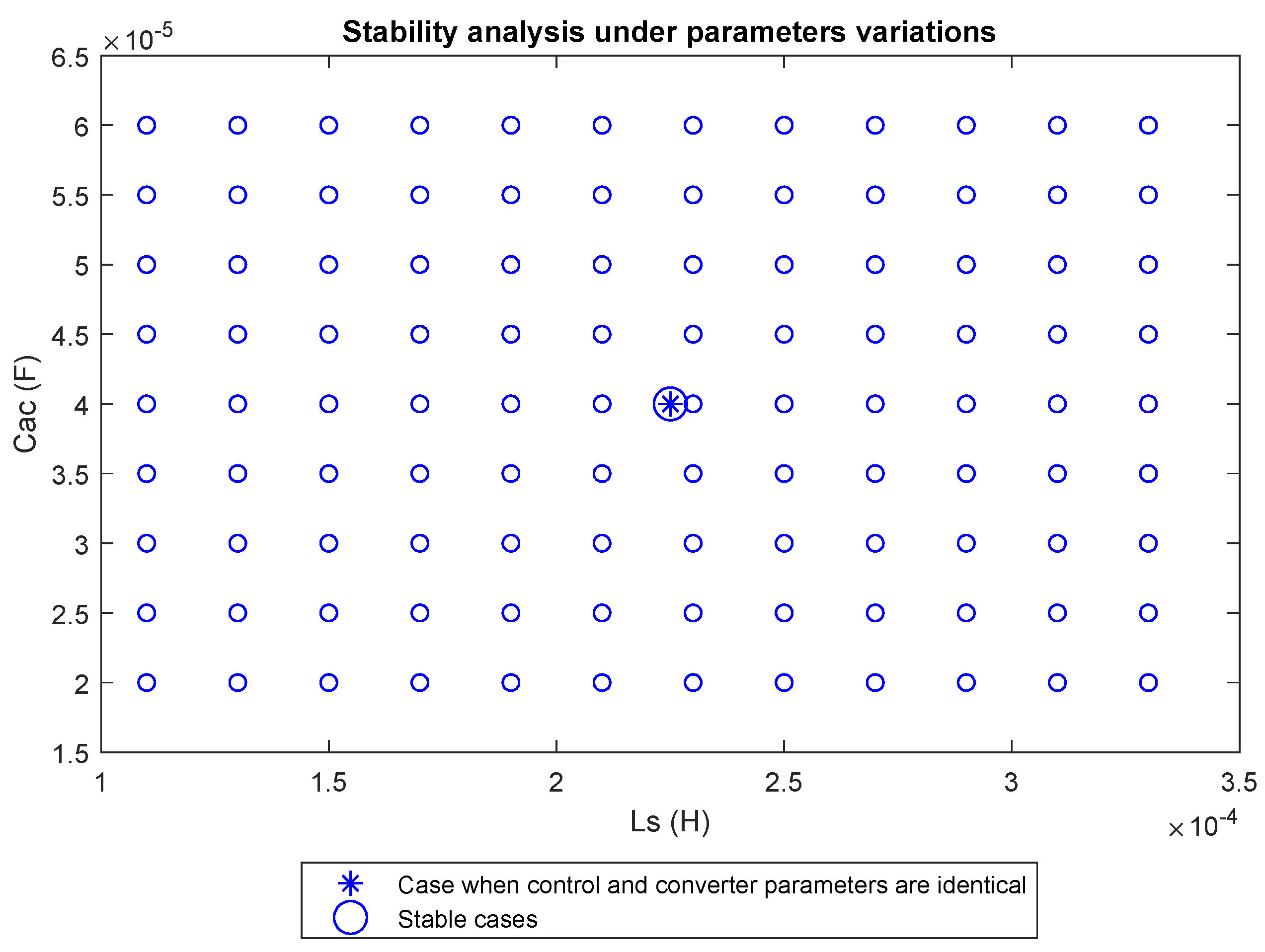
We will study the stability of the system with variations of the AC filter parameters (C and ). Indeed, these values can change during operation and time. To realize this study, control laws will use constant values of F and H, while system values will be increased, respectively, from F to F and from H to H. The other parameters used to realize this test are listed in Table 1 and Table 3.
Figure 7 presents the stability analysis of the system in a closed loop with parameter variations. Errors on AC filter parameters are introduced and the sign of eigenvalues are studied to make conclusions on the stability of each point.
We found that even with errors on both values of the AC filter, the system remains stable because all the eigenvalues have a negative real part.
5. Simulation Results
Table 1 and Table 4 display the control parameters which will be used for the simulation and experimental tests.
Table 3 shows the parameters of the buck-type current-source rectifier used in the simulation and the experimental tests.
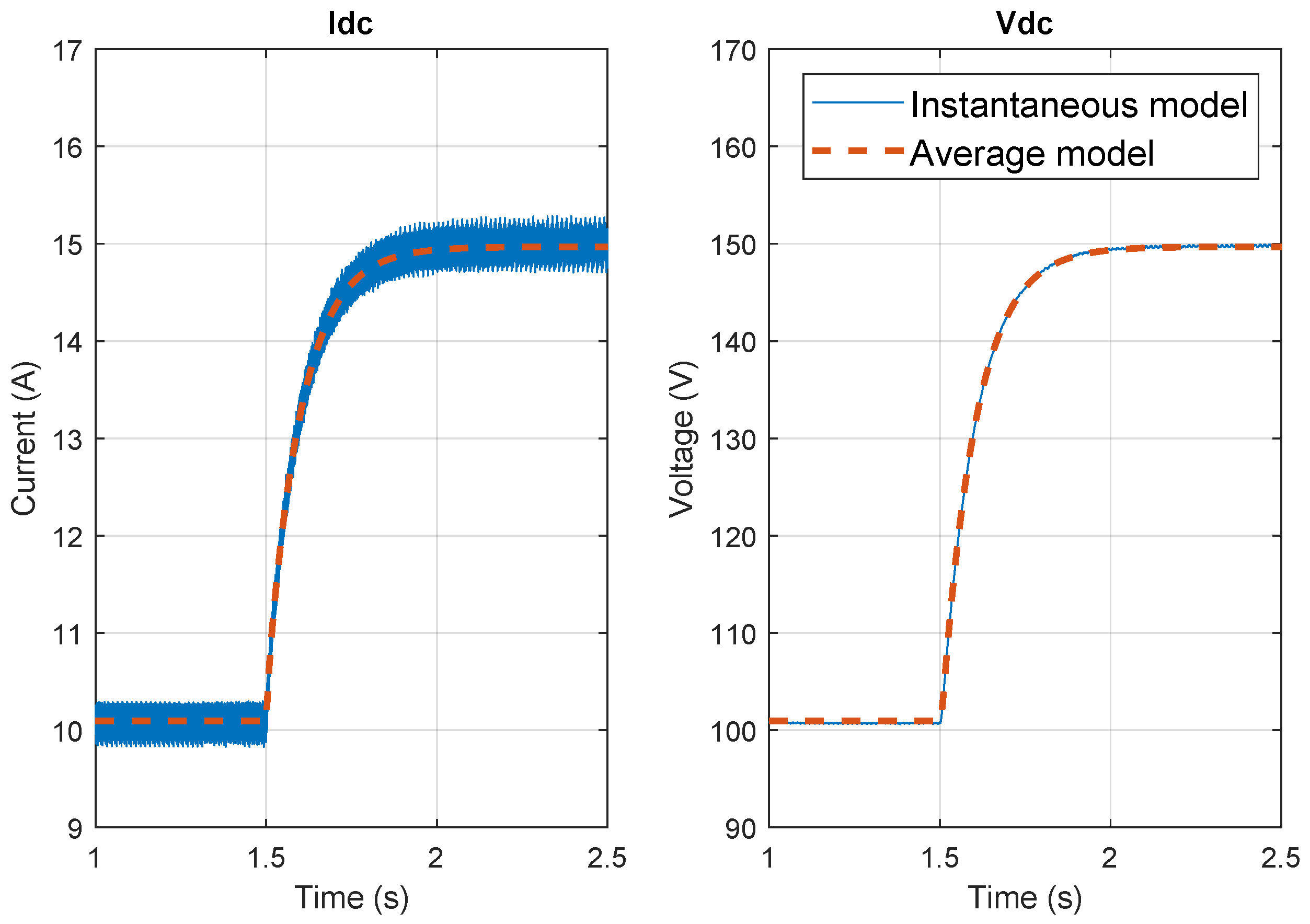
In Figure 8, the simulation of the instantaneous model with SVM and the one of the average models are carried out, when the system is in an open loop (meaning that the values for both control variables and are set directly). Both simulations show the same dynamic behavior, which validates the approximation of the average model.
To ensure good continuity of service of the electrolyzer, the DC-output voltage of the rectifier has to be maintained as much as possible during a sudden voltage drop of the network. The simulation (using the average model) of the system during a drop of the rms grid voltage (reduction from 55 V to 40 V) is displayed in Figure 9 and Figure 10 for an electrolyzer with 25 cells in series (2 V at the terminals of each cell).
Figure 11 shows the system behavior for grid voltage reduction from 110 V to 90 V for an electrolyzer with 50 cells in series (2 V at the terminals of each cell). The system remains stable during the disturbance: this one is removed quickly after 50 ms. There is a transient voltage drop on the DC system of about 5 V in both cases, followed by a minor overvoltage. The DC current oscillation is about 1A in both cases.
Figure 10 displays the influence of the value of the control parameter on the output voltage . It can be seen that the higher the value of is, the faster the disturbance is removed. In addition, it is important to notice that a high value of generates a lower voltage drop.
A simulation is performed to compare the classical control using two cascaded PI controllers with and without the presence of an active damping method with the proposed solution. PI controllers can be written as follows for the current and voltage loops:
The active damping method used consists of emulating a damping resistor, without any additional power loss by making the CSR produce an additional current added to the reference current of the d axis (). It is based on the voltage measurement across the AC capacitor. After using a high pass filter to keep only the alternative part, the obtained voltage is divided by the virtual resistor to generate the damping current [34].
The points of comparison will be: the magnitude of the oscillations on the grid current in steady state and the performances under disturbances generated by a resistive load whose value is changed from to . The two controllers are tuned to obtain the same bandwidth in a closed loop in each case. Two cases are presented with each control corresponding to different settings: one is relatively slow (cutoff frequency of the voltage loop is 85 rad·s) and one is relatively fast (cutoff frequency of the voltage loop is 175 rad·s.
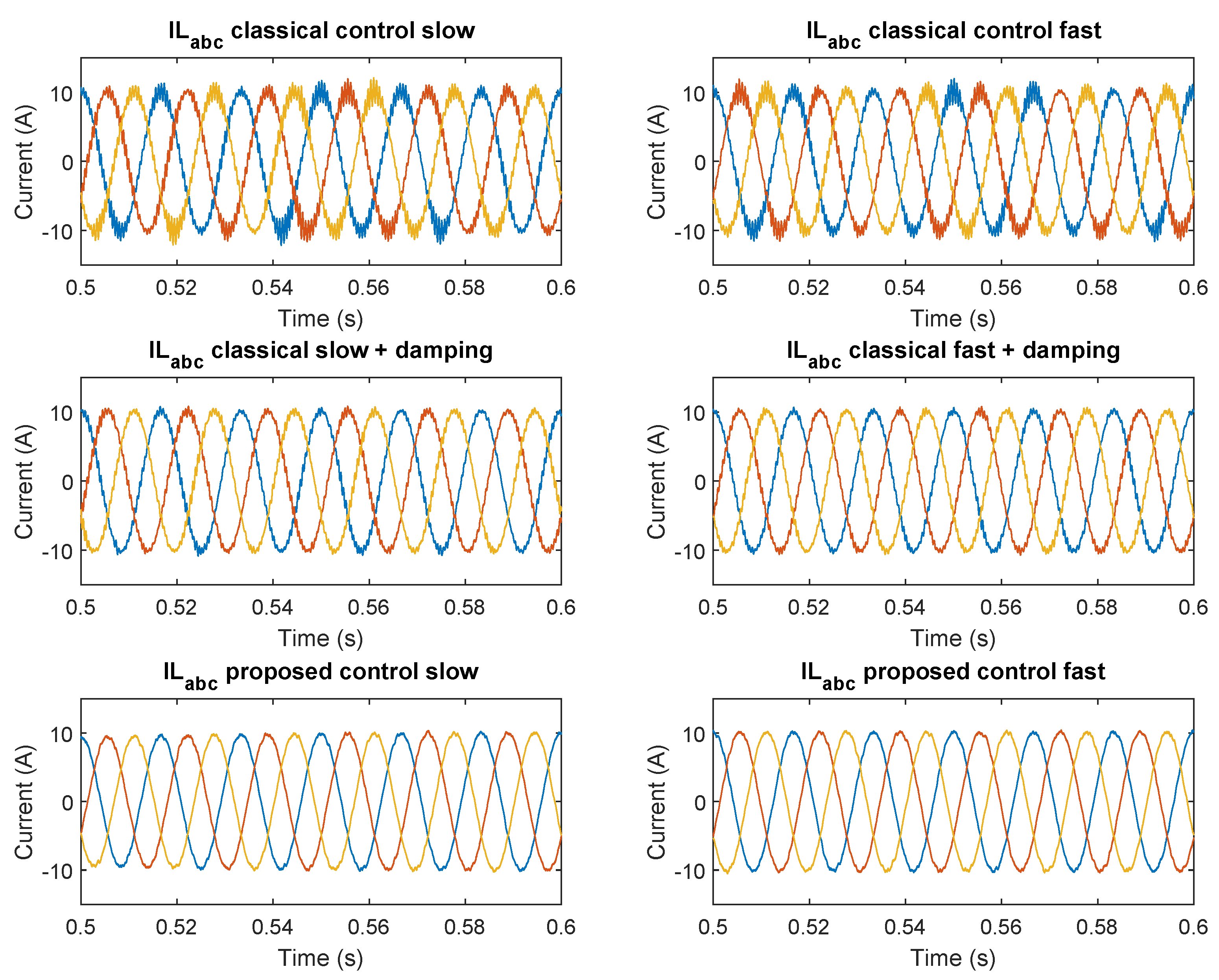
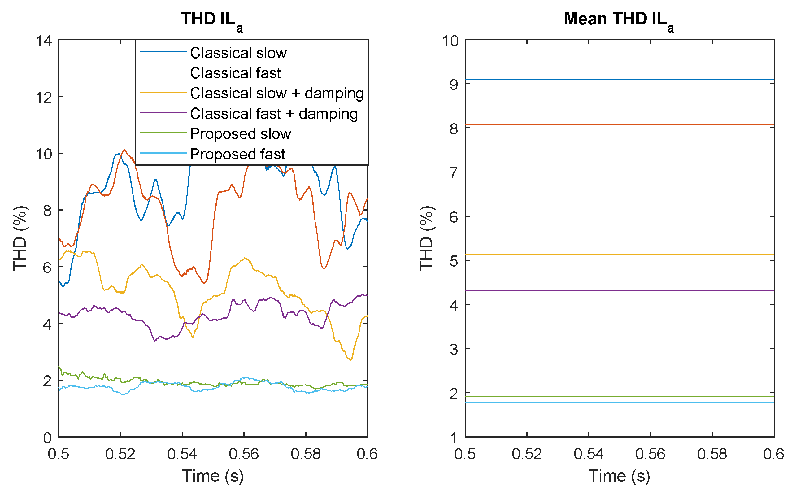
In Figure 12, it is possible to see the grid current in steady state with: the classical control without an active damping method (top), the classical control with an active damping method (middle), and the proposed control (bottom). Converter parameters are listed in Table 3 with a voltage grid at 110 V and a resistive load of . Control parameters are listed in Table 1 and Table 4. Controllers are tuned to be slow on the left side and fast on the right side. It is possible to highlight that the presence of an active damping method reduces the magnitude of oscillations (from 3A to 1A) compared to the solution without. However, the proposed control shows a greater reduction of the magnitude of oscillations (from 3 A to 0.15 A). In addition, to highlight this result, the Total Harmonics Distorsion (THD) has been computed in the different cases and presented in Figure 13. It appears that the proposed solution has the lowest THD value of the grid current.
The behavior of the system subjected to a sudden change of the load has been tested. A comparison between the classical control with and without the active damping method is first presented in Figure 14. This figure confirms that the introduction of the damping method does not affect the dynamic behavior of the control. Next, a comparison between the classical and the proposed control is given in Figure 15. The classical and the proposed solutions are compared in two cases depending on the tuning of the control parameters. One case is considered as slow and the other as fast.
In the first case where the controllers are slow, the overvoltage on is reduced from 50 V to 30 V with the proposed solution. Additionally, the voltage drop with the classical control is about 10 V when there is no voltage drop with the proposed control. Regarding the output current, , there is a current drop of about 1.5 A with the classical control, while it is equal to zero with the proposed control.
In the second case where the controllers are faster, with the proposed control, the overvoltage on is reduced from 32 V to 22 V. Additionally, while there is no voltage drop with the proposed control, the voltage drop with the classical control is about 5 V. In this case, with the proposed control, the current drop on is not eliminated, but reduced from 1.5 A to 0.8 A.
From these results (resumed in Table 5), it is then possible to see that in both cases (slow and fast), the proposed control shows better dynamic performances compared to the classical solution. Furthermore, it allows one to reduce the magnitude of the grid current oscillations, which leads to an improvement in the value of the grid current THD.
6. Experimental Results
In order to verify the proposed solution, a test bench has been set up as shown in Figure 16.
It is first composed of a three-phase controllable AC source Chroma 61702. Second, a MicroLabBox DS1202 is used with Matlab/Simulink and ControlDesk to monitor the state variables of the system and compute the reference variables. Next, these variables are sent to a FPGA DE0-Nano, which is responsible for sending command signals to the semi-conductors using optical fibers. The FPGA has been programmed using Quartus software in VHDL language. Finally, the system also includes an active load (EA Elektro-Automatik 9750-22) that can be controlled with analog inputs directly coming from the DAC port (Digital Analog Converter) of the MicroLabBox.
The quasi-static characteristic of an electrolyzer has been implemented in the active load. This characteristic allows us to emulate the behavior of a selected electrolyzer and establish the operating point according to the voltage imposed on its terminals. A typical characteristic of one cell is presented in Figure 17: it displays the current density (A/cm) as a function of the voltage (V) across the cell. A stack corresponds to an association between serial and parallel cells. In this study, the surface is selected at around 7 cm with 50 cells in series for Test I and Test II, and 25 cells in series for Test III. The power extracted by the electrolyzer as a function of the voltage at its terminals is shown in Figure 17. In order to extract the maximum power while maintaining the electrolyzer in good conditions, it was decided to apply 2 V to the terminals of each cell as an operating point for Test I and Test III. Another operating point has been tested with Test II, corresponding to 1.8 V to the terminal of each cell.
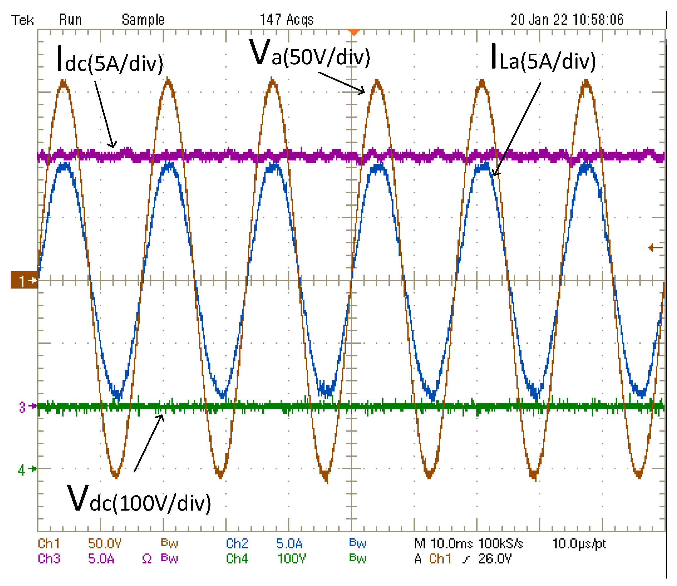
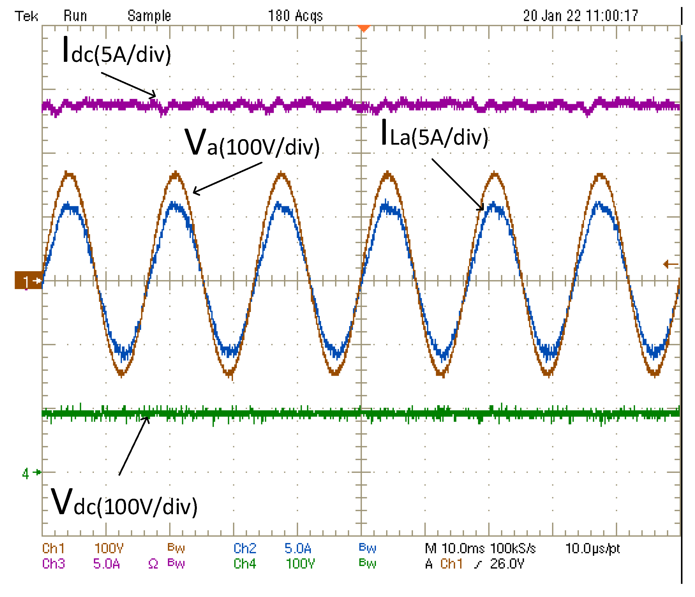
Figure 18 and Figure 19 present the behavior of the system in steady-state with the proposed control during Test I and Test II. The parameters during these tests are indicated in Table 1, Table 2 and Table 3. In these figures, it is possible to see the grid voltage , the grid current , the output current , and the output voltage . It can be seen that grid voltage, , and current, , are in phase. It means that the reactive power, coming in particular from the differential mode input, , filter is totally compensated. The proposed control makes it possible to operate with a unit power factor. In addition, the oscillations on the grid current are damped using the proposed control without the need of any damping element or virtual active damping control.
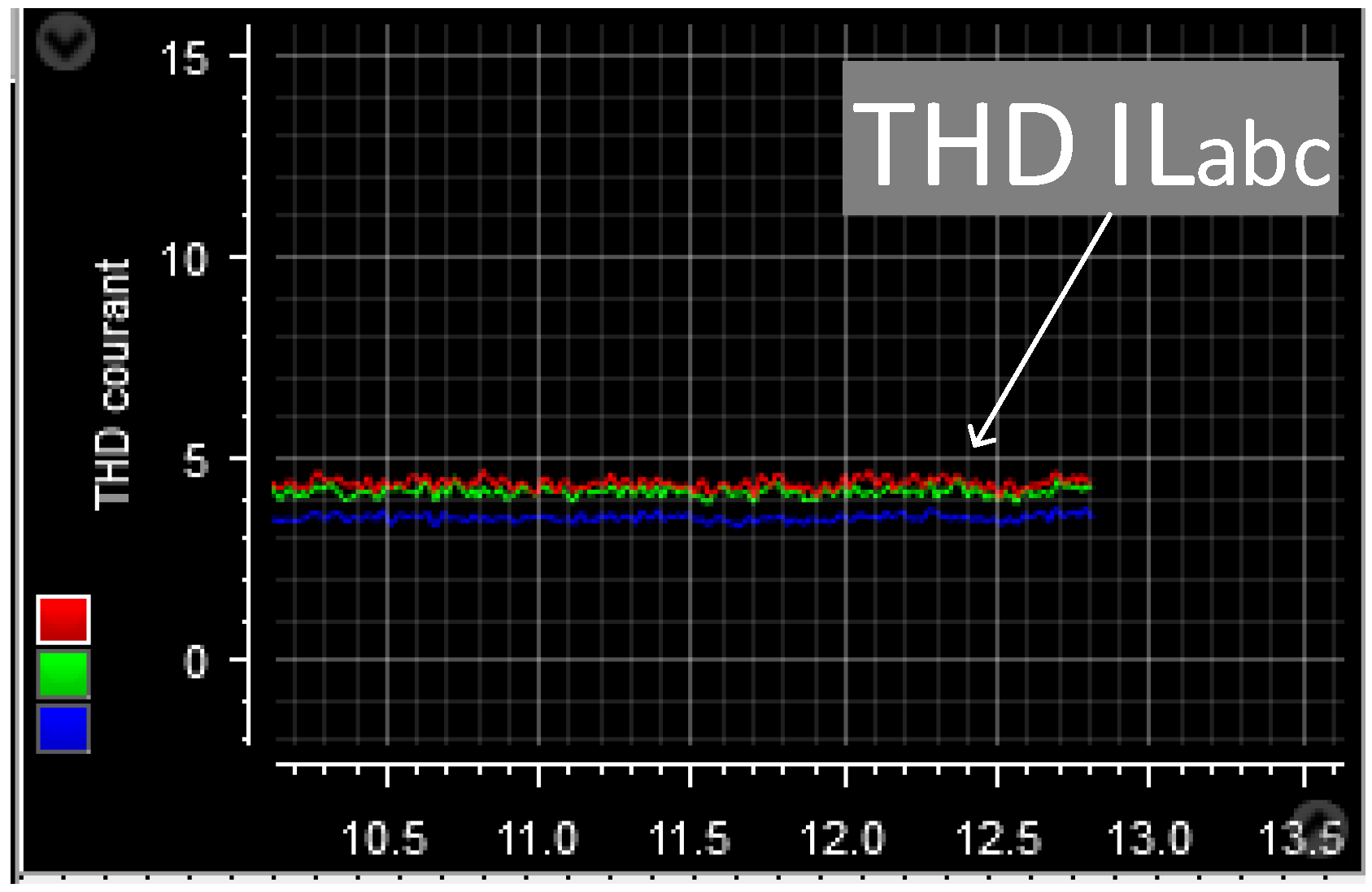
Figure 20 displays the behavior of the system in a steady state with the proposed control during Test III. The parameters during this test are shown in Table 1 and Table 2. We obtain the same results as in Test I and Test II: no oscillations on the grid current, grid voltage and current are in phase, and there are low ripples on the output current. In Figure 21, it is possible to see the value of the THD of the grid current during the test. The definition chosen for the THD is the ratio between the amplitude of the harmonics and the fundamental value of the signal (Total Harmonic Distortion compared to the fundamental). Here, it is less than , which indicates a grid current with very few disturbances in the network induced by the rectifier.
It is important, in order to guarantee a good continuity of service of the electrolyzer, to maintain the desired voltage at its terminals, for example during a micro-cut of the electrical network, i.e., during a sudden variation of its rms voltage. In order to study the response of the system during a sudden drop in the rms voltage of the network, Test III was carried out. In Figure 22, it is possible to see the grid voltages, , the output current, , and voltage, , during a sudden drop of the rms grid voltage from 55 V to 40 V with two different values of . The system remains stable and the desired output voltage is maintained in both cases. Further, as in simulation (Figure 9), it appears that a high value of , allows one to reduce the voltage drop (7 V instead of 9 V) and removes the perturbation rapidly (50 ms instead of 100 ms).
The simulation corresponding to Test III was displayed in Figure 9. The behavior of the system is similar between the simulation and experimental tests; for example, with = 120 rad·s, the DC transient voltage drop is about 7 V (5 V by simulation) and the current drop 1.25 A (1.2A by simulation). The DC current exceeding the set value is less than that in the simulation: it appears to be damped. It may be explained by modeling errors or a misidentification of parameters, but also the way in which the rms voltage drop is generated.
7. Conclusions
AC microgrids, composed of several renewable energy sources and several loads, need solutions to regulate the power produced as a function of the power consumed. To cope with the intermittency of these sources, ESS based on the electrolysis of water to produce hydrogen is a popular option. To improve the connection of the electrolyzer to the AC grid, the use of a single-stage conversion, three-phase buck-type rectifier has been evaluated.
First, an average model to model the rectifier has been described. Simulation times are faster than those of the instantaneous model (since it does not require the SVM part) without altering the system dynamics.
Next, we proposed a new control of this converter based on the flatness properties of the differential systems. It allows one to control the oscillations of the input filter without using active damping method and guarantees the large signal stability of the converter. The proposed solution is easy to tune, does not depend on the operating point, and presents better results regarding oscillation mitigation and dynamic performance than the classical control with active damping.
A simulation and experimental tests have been carried out to prove the efficiency of the solution. An active load has been used to emulate the electrolyzer, described by its quasi-static characteristic. In a steady state, the unitary power factor was achieved. Further, the THD of the grid current is kept low () during operation.
Finally, the behavior of the converter has been studied under a sudden drop of the rms grid voltage. We noticed that the converter remains stable and removes the perturbation quickly. This allows one to maintain the operating condition of the electrolyzer and guarantees a good continuity of service.
The proposed solution is a suitable one-stage conversion option to use the excess of electricity production to store hydrogen based on water electrolysis, to maintain a constant voltage at the terminals of the electrolyzer in the case of a grid disturbance, all while the grid current is stabilized with a unity power factor.
Author Contributions
Conceptualization, S.P.; data curation, Q.C.; formal analysis, Q.C., A.A. and S.P.; investigation, Q.C.; methodology, Q.C.; project administration, S.P.; resources, M.W.; software, Q.C. and M.W.; supervision, S.D.; validation, S.D.; Writing—original draft, Q.C.; Writing—review & editing, Q.C. All authors have read and agreed to the published version of the manuscript.
Funding
This research was supported by the Région Grand Est, France.
Conflicts of Interest
The authors declare no conflict of interest.
References
- Hu, J.; Shan, Y.; Guerrero, J.M.; Ioinovici, A.; Chan, K.W.; Rodriguez, J. Model predictive control of microgrids—An overview. Renew. Sustain. Energy Rev. 2021, 136, 110422. [Google Scholar] [CrossRef]
- Abdalla, A.N.; Nazir, M.S.; Tao, H.; Cao, S.; Ji, R.; Jiang, M.; Yao, L. Integration of energy storage system and renewable energy sources based on artificial intelligence: An overview. J. Energy Storage 2021, 40, 102811. [Google Scholar] [CrossRef]
- Justo, J.J.; Mwasilu, F.; Lee, J.; Jung, J.W. AC-microgrids versus DC-microgrids with distributed energy resources: A review. Renew. Sustain. Energy Rev. 2013, 24, 387–405. [Google Scholar] [CrossRef]
- Guilbert, D.; Vitale, G. Improved hydrogen-production-based power management control of awind turbine conversion system coupled with multistack proton exchange membrane electrolyzers. Energies 2020, 13, 1239. [Google Scholar] [CrossRef] [Green Version]
- Eroǧlu, F.; Kurtoǧlu, M.; Vural, A.M. Bidirectional DC–DC converter based multilevel battery storage systems for electric vehicle and large-scale grid applications: A critical review considering different topologies, state-of-charge balancing and future trends. IET Renew. Power Gener. 2021, 15, 915–938. [Google Scholar] [CrossRef]
- Guida, V.; Guilbert, D.; Vitale, G.; Douine, B. Design and Realization of a Stacked Interleaved DC–DC Step-Down Converter for PEM Water Electrolysis with Improved Current Control. Fuel Cells 2020, 20, 307–315. [Google Scholar] [CrossRef]
- Valencia, G.; Benavides, A.; Cárdenas, Y. Economic and environmental multiobjective optimization of a wind-solar-fuel cell hybrid energy system in the Colombian Caribbean region. Energies 2019, 12, 2119. [Google Scholar] [CrossRef] [Green Version]
- Hernández-Gómez, Á.; Ramirez, V.; Guilbert, D.; Saldivar, B. Development of an adaptive static-dynamic electrical model based on input electrical energy for PEM water electrolysis. Int. J. Hydrogen Energy 2020, 45, 18817–18830. [Google Scholar] [CrossRef]
- Concha, D.; Renaudineau, H.; Hernández, M.S.; Llor, A.M.; Kouro, S. Evaluation of DCX converters for off-grid photovoltaic-based green hydrogen production. Int. J. Hydrogen Energy 2021, 46, 19861–19870. [Google Scholar] [CrossRef]
- Yodwong, B.; Guilbert, D.; Phattanasak, M.; Kaewmanee, W.; Hinaje, M.; Vitale, G. AC-DC converters for electrolyzer applications: State of the art and future challenges. Electronics 2020, 9, 912. [Google Scholar] [CrossRef]
- Speckmann, F.W.; Bintz, S.; Birke, K.P. Influence of rectifiers on the energy demand and gas quality of alkaline electrolysis systems in dynamic operation. Appl. Energy 2019, 250, 855–863. [Google Scholar] [CrossRef]
- Koponen, J.; Ruuskanen, V.; Kosonen, A.; Niemela, M.; Ahola, J. Effect of Converter Topology on the Specific Energy Consumption of Alkaline Water Electrolyzers. IEEE Trans. Power Electron. 2019, 34, 6171–6182. [Google Scholar] [CrossRef]
- Rodríguez, J.R.; Pontt, J.; Silva, C.; Wiechmann, E.P.; Hammond, P.W.; Santucci, F.W.; Álvarez, R.; Musalem, R.; Kouro, S.; Lezana, P. Large current rectifiers: State of the art and future trends. IEEE Trans. Ind. Electron. 2005, 52, 738–746. [Google Scholar] [CrossRef]
- Solanki, J.; Fröhleke, N.; Böcker, J.; Averberg, A.; Wallmeier, P. High-current variable-voltage rectifiers: State of the art topologies. IET Power Electron. 2015, 8, 1068–1080. [Google Scholar] [CrossRef]
- Sayed, K.; Gronfula, M.G.; Ziedan, H.A. Novel soft-switching integrated boost DC-DC converter for PV power system. Energies 2020, 13, 749. [Google Scholar] [CrossRef] [Green Version]
- Choi, S.S.; Lee, C.W.; Kim, I.D.; Jung, J.H.; Seo, D.H. New Induction Heating Power Supply for Forging Applications Using IGBT Current-Source PWM Rectifier and Inverter. In Proceedings of the ICEMS 2018—2018 21st International Conference on Electrical Machines and Systems, Jeju, Korea, 7–10 October 2018; pp. 709–713. [Google Scholar] [CrossRef]
- Wei, Q.; Wu, B.; Xu, D.; Zargari, N.R. A New Configuration Using PWM Current Source Converters in Low-Voltage Turbine-Based Wind Energy Conversion Systems. IEEE J. Emerg. Sel. Top. Power Electron. 2018, 6, 919–929. [Google Scholar] [CrossRef]
- Zhang, D.; Guacci, M.; Haider, M.; Bortis, D.; Kolar, J.W.; Everts, J. Three-Phase Bidirectional Buck-Boost Current DC-Link EV Battery Charger Featuring a Wide Output Voltage Range of 200 to 1000 V. In Proceedings of the ECCE 2020—IEEE Energy Conversion Congress and Exposition, Detroit, MI, USA, 11–15 October 2020; pp. 4555–4562. [Google Scholar] [CrossRef]
- Gutierrez, B.; Kwak, S.S. Cost-effective matrix rectifier operating with hybrid bidirectional switch configuration based on Si IGBTs and SiC MOSFETs. IEEE Access 2020, 8, 136828–136842. [Google Scholar] [CrossRef]
- Migliazza, G.; Buticchi, G.; Carfagna, E.; Lorenzani, E.; Madonna, V.; Giangrande, P.; Galea, M. DC Current Control for a Single-Stage Current Source Inverter in Motor Drive Application. IEEE Trans. Power Electron. 2021, 36, 3367–3376. [Google Scholar] [CrossRef]
- Akbar, F.; Cha, H.; Do, D.t. CSI7: Novel Three-Phase Current-Source Inverter. IEEE Trans. Power Electron. 2021, 36, 9170–9182. [Google Scholar] [CrossRef]
- Torres, R.A.; Dai, H.; Lee, W. Current-Source Inverter Integrated Motor Drives using Dual-Gate Four-Quadrant Wide-Bandgap Power Switches. IEEE Trans. Ind. Appl. 2021, 57, 5183–5198. [Google Scholar] [CrossRef]
- Saber, C.; Labrousse, D.; Revol, B.; Gascher, A. Challenges Facing PFC of a Single-Phase On-Board Charger for Electric Vehicles Based on a Current Source Active Rectifier Input Stage. IEEE Trans. Power Electron. 2016, 31, 6192–6202. [Google Scholar] [CrossRef] [Green Version]
- Gao, H.; Wu, B.; Xu, D.; Zargari, N.R. A Model Predictive Power Factor Control Scheme with Active Damping Function for Current Source Rectifiers. IEEE Trans. Power Electron. 2018, 33, 2655–2667. [Google Scholar] [CrossRef]
- Guo, X.; Yang, Y.; Wang, B.; Lu, Z. Generalized Space Vector Modulation for Current Source Converter in Continuous and Discontinuous Current Modes. IEEE Trans. Ind. Electron. 2020, 67, 9348–9357. [Google Scholar] [CrossRef]
- Saber, C. Analysis and Optimization of the Conducted Emissions of an On-Board Charger for Electric Vehicles to Cite This Version: Analysis and Optimization of the Conducted Emissions of an On-Board Charger for Electric Vehicles Analyse et Optimisation de la CEM. Ph.D. Thesis, Université Paris Saclay, Gif-sur-Yvette, France, 2017. [Google Scholar]
- Kolar, J.W.; Friedli, T. The essence of three-phase PFC rectifier systems Part I. IEEE Trans. Power Electron. 2013, 28, 176–198. [Google Scholar] [CrossRef]
- Li, X.; Wu, F.; Yang, G.; Liu, H.; Meng, F. Precise Calculation Method of Vector Dwell Times for Single-Stage Isolated Three-Phase Buck-Type Rectifier to Reduce Grid Current Distortions. IEEE J. Emerg. Sel. Top. Power Electron. 2020, 8, 4457–4466. [Google Scholar] [CrossRef]
- Wei, Q.; Xing, L.; Xu, D.; Wu, B.; Zargari, N.R. Modulation Schemes for Medium-Voltage PWM Current Source Converter-Based Drives: An Overview. IEEE J. Emerg. Sel. Top. Power Electron. 2019, 7, 1152–1161. [Google Scholar] [CrossRef]
- Fliess, M.; Levine, J.; Martin, P.; Rouchon, P. Flatness and defect of non-linear systems: Introductory theory and examples. Int. J. Control 1995, 61, 1327–1361. [Google Scholar] [CrossRef] [Green Version]
- Thounthong, P.; Sikkabut, S.; Poonnoy, N.; Mungporn, P.; Yodwong, B.; Kumam, P.; Bizon, N.; Nahid-Mobarakeh, B.; Pierfederici, S. Nonlinear Differential Flatness-Based Speed/Torque Control with State-Observers of Permanent Magnet Synchronous Motor Drives. IEEE Trans. Ind. Appl. 2018, 54, 2874–2884. [Google Scholar] [CrossRef]
- Huangfu, Y.; Li, Q.; Xu, L.; Ma, R.; Gao, F. Extended State Observer Based Flatness Control for Fuel Cell Output Series Interleaved Boost Converter. IEEE Trans. Ind. Appl. 2019, 55, 6427–6437. [Google Scholar] [CrossRef]
- Zandi, M.; Gavagsaz Ghoachani, R.; Phattanasak, M.; Martin, J.P.; Nahidmobarakeh, B.; Pierfederici, S.; Davat, B.; Payman, A. Flatness based control of a non-ideal DC/DC boost converter. In Proceedings of the IECON Proceedings (Industrial Electronics Conference), Toronto, ON, Canada, 13–16 October 2011; pp. 1360–1365. [Google Scholar] [CrossRef]
- Zhang, Y.; Yi, Y.; Dong, P.; Liu, F.; Kang, Y. Simplified Model and Control Strategy of Three-Phase PWM Current Source Rectifiers for DC Voltage Power Supply Applications. IEEE J. Emerg. Sel. Top. Power Electron. 2015, 3, 1090–1099. [Google Scholar] [CrossRef]
Figure 1.
AC microgrid structure.

Figure 2.
Energy conversion systems used to power an electrolyzer.

Figure 3.
Buck-type current-source rectifier.

Figure 4.
PWM pattern.

Figure 5.
Space Vector Modulation.

Figure 6.
General control scheme.

Figure 7.
Stability analysis under parameter variations (inductance and capacity of AC filters are changed). Parameters are listed in Table 1 and Table 3, and the operating point corresponds to Test I in Table 2.

Figure 8.
Comparison between the instantaneous model with SVM and the average model in an open loop with the parameters of Table 3 when the voltage reference is increased from 100 V to 150 V on a resistive load with a voltage grid at 110 V.
Figure 8.
Comparison between the instantaneous model with SVM and the average model in an open loop with the parameters of Table 3 when the voltage reference is increased from 100 V to 150 V on a resistive load with a voltage grid at 110 V.

Figure 9.
Simulation results when the rms grid voltage drops from 55 V to 40 V with an ouptut voltage regulation at 50 V: grid voltages on the (left), output voltage in the center, and output current on the (right). Parameters are listed in Table 1 and Table 3.

Figure 10.
Simulation results: influence of the value of on the output voltage when the rms grid voltage drops from 55 V to 40 V with the output voltage regulation at 50 V. Parameters are listed in Table 1 and Table 3.

Figure 11.
Simulation results when the rms grid voltage drops from 110 V to 90 V with an ouptut voltage regulation at 100 V: grid voltages on the (left), output voltage in the center, and output current on the (right). Parameters are listed in Table 1 and Table 3.

Figure 12.
Simulation results: grid current in a steady state with the classical control without a damping method (top), with a damping method (middle), and with the proposed control (bottom) regarding the magnitude of the oscillations. Grid voltage is at 110 V with a resistive load. Other parameters are listed in Table 3 and Table 4.

Figure 13.
Simulation results: THD (%) of the grid current (phase a) in the different cases. Grid voltage is at 110 V with a resistive load. Parameters are listed in Table 3 and Table 4.

Figure 14.
Simulation results of the classical control with and without active damping method: behavior of the output current () and voltage () during a load step from to . Grid voltage is at 110 V. Parameters are listed in Table 3 and Table 4.

Figure 15.
Simulation results of the classical control with damping method and the proposed control: behavior of the output current () and voltage () during a load step from to . Grid voltage is at 110 V. Parameters are listed in Table 3 and Table 4.

Figure 16.
Experimental setup.

Figure 17.
Typical characteristic of a PEM cell (left) and power as a function of voltage across a stack of 50 cells in series (right).
Figure 17.
Typical characteristic of a PEM cell (left) and power as a function of voltage across a stack of 50 cells in series (right).

Figure 18.
Experimental results in a steady state when the voltage at the terminals of each cell (50 cells in series) is set to 2 V. Test I (Table 2) with parameters in Table 1 and Table 3.

Figure 19.
Experimental results in a steady state when the voltage at the terminals of each cell (50 cells in series) is set to 1.8 V. Test II (Table 2) with parameters in Table 1 and Table 3.

Figure 20.
Experimental results during Test III (Table 2) when 2 V are applied at the terminals of each cell (25 cells in series) with parameters listed in Table 1 and Table 3.

Figure 21.
THD (%) of the grid current in a steady state (0% corresponds to no harmonics).

Figure 22.
Experimental results (Test III (Table 2)) when the grid voltage is reduced from 55 V to 40 V with = 120 rad·s (top) and = 50 rad·s (bottom).
Figure 22.
Experimental results (Test III (Table 2)) when the grid voltage is reduced from 55 V to 40 V with = 120 rad·s (top) and = 50 rad·s (bottom).


Table 1.
Control parameters.
| Notations | Value | Unity |
|---|---|---|
| - | ||
| 50–120 | rad·s | |
| 6000 | rad·s | |
| 6000 | rad·s | |
| Notations | slow case | fast case |
| 85 rad·s | 175 rad·s |
Table 2.
Experimental parameters.
| Parameters | Notations | Value Test I | Value Test II | Value Test III |
|---|---|---|---|---|
| Grid voltage | 110 V | 110 V | 55 V | |
| Output DC voltage | 100 V | 93 V | 50 V | |
| Output DC current | 20A | 13A | 10A | |
| Grid frequency | f | 60 Hz | 60 Hz | 60 Hz |
| Efficiency |
Table 3.
Parameters of the buck-type current-source rectifier.
| Parameters | Notations | Value |
|---|---|---|
| Grid frequency | f | 60 Hz |
| DC capacitor | 0.94 mF | |
| Filter’s inductance | 225 H | |
| AC series resistance | ||
| Filter’s capacitance | C | 39 F |
| Output inductance | 9.7 mH | |
| DC series resistance |
Table 4.
PI control parameters.
| Notations | Slow Case | Fast Case |
|---|---|---|
| 0.5 | 1 | |
| 900 | 800 | |
| 0.04 | 0.1 | |
| 180 | 180 |
Table 5.
Simulation results of the different methods regarding the magnitude of oscillations in steady-state and dynamic performances during a load step from to .
Table 5.
Simulation results of the different methods regarding the magnitude of oscillations in steady-state and dynamic performances during a load step from to .
| Slow Setting | Fast Setting | |||||
|---|---|---|---|---|---|---|
| Classical Control without Damping | Classical Control with Damping | Proposed Control | Classical Control without Damping | Classical Control with Damping | Proposed Control | |
| Magnitude of grid current oscillations (A) | 3 | 1 | 0.15 | 3.5 | 1 | 0.15 |
| Overvoltage (V) | 50 | 50 | 30 | 32 | 32 | 22 |
| Voltage drop (V) | 10 | 10 | - | 5 | 5 | - |
| Current drop (A) | 1.5 | 1.5 | - | 1.5 | 1.5 | 0.8 |
| Grid current THD (%) (averaged) | 9.1 | 5.1 | 1.9 | 8.1 | 4.3 | 1.8 |
Publisher’s Note: MDPI stays neutral with regard to jurisdictional claims in published maps and institutional affiliations. |
© 2022 by the authors. Licensee MDPI, Basel, Switzerland. This article is an open access article distributed under the terms and conditions of the Creative Commons Attribution (CC BY) license (https://creativecommons.org/licenses/by/4.0/).
Share and Cite
MDPI and ACS Style
Combe, Q.; Abasian, A.; Pierfederici, S.; Weber, M.; Dufour, S. Control of a Three-Phase Current Source Rectifier for H2 Storage Applications in AC Microgrids. Energies 2022, 15, 2436. https://0-doi-org.brum.beds.ac.uk/10.3390/en15072436
AMA Style
Combe Q, Abasian A, Pierfederici S, Weber M, Dufour S. Control of a Three-Phase Current Source Rectifier for H2 Storage Applications in AC Microgrids. Energies. 2022; 15(7):2436. https://0-doi-org.brum.beds.ac.uk/10.3390/en15072436
Chicago/Turabian StyleCombe, Quentin, Alireza Abasian, Serge Pierfederici, Mathieu Weber, and Stéphane Dufour. 2022. "Control of a Three-Phase Current Source Rectifier for H2 Storage Applications in AC Microgrids" Energies 15, no. 7: 2436. https://0-doi-org.brum.beds.ac.uk/10.3390/en15072436
Note that from the first issue of 2016, this journal uses article numbers instead of page numbers. See further details here.