
Research on TVD Control of Cornering Energy Consumption for Distributed Drive Electric Vehicles Based on PMP


1
College of Automotive Engineering, Changzhou Institute of Technology, Changzhou 213001, China
2
School of Mechanical and Aerospace Engineering, Queen’s University Belfast, Belfast BT7 1NN, UK
3
State Key Laboratory of Automotive Simulation and Control, Jilin University, Changchun 130022, China
*
Author to whom correspondence should be addressed.
Energies 2022, 15(7), 2641; https://0-doi-org.brum.beds.ac.uk/10.3390/en15072641
Submission received: 27 February 2022
/
Revised: 28 March 2022
/
Accepted: 1 April 2022
/
Published: 4 April 2022
(This article belongs to the Collection State of the Art Electric Vehicle Technology in China)
Abstract
:This paper aims to study the torque optimization control of distributed drive electric vehicles in the cornering process and reduce the cornering energy consumption. The main energy consumption of the vehicle in the cornering process is analyzed clearly based on the 7-DOF vehicle dynamics model. The torque vectoring distribution (TVD) of a distributed drive electric vehicle in the process of turning was studied on the basis of the Pontryagin Minimum Principle (PMP). The Beetle Antenna Search–Particle Swarm Optimization (BAS-PSO) algorithm was used to optimize the torque distribution coefficient offline, and the algorithm was improved to improve the operation speed. Based on the vehicle dynamics characteristics, the table of torque distribution coefficient of minimum turning energy consumption and the optimal energy-saving degree of TVD control in different bending conditions were worked out.
1. Introduction
Energy depletion and environmental pollution are limiting the development of the world. As one of the high-tech products of today’s social development and technological innovation, the reduction in energy consumption and pollution in the process of use has been the focus of the industry. Developing and innovating new energy vehicle technology vigorously has become a trend in this industry all over the world [1].
In the field of new energy vehicle technology, the important position is firmly occupied by distributed drive electric vehicles, which have the outstanding advantages of short drive chain, high transmission efficiency, and compact structure [2]. The driving motors are directly installed in the driving wheels or near the driving wheels, which is their main structural feature. The motor is not only the power unit of the vehicle but also the control execution unit with fast response. The various dynamic control functions of the vehicle are easily realized by controlling the driving or braking torque of the independent motor [3,4]. An important aspect of the current research on the TVD control technology of a distributed drive system is to improve the lateral stability of the vehicle. Finally, the handling stability and fuel economy of the vehicle will be improved [5].
With the development of the city, road condition information gradually tends to become more complex and varied. The contribution of energy-saving efficiency of straight-line driving to the total energy-saving efficiency of vehicles is also getting lower and lower. Therefore, greater emphasis has been placed on the energy efficiency of turning driving conditions. In the research of distributed drive electric vehicle technologies, the reduction in vehicle energy consumption can be easily achieved by torque directional distribution control technology, and the vehicle economy will be greatly improved [6]. For TVD technology, many well-known scholars and experts worldwide have proposed related technologies to improve vehicle-handling stability. Oh et al. [7] introduced a yaw stability control algorithm of a four-wheel drive vehicle based on physical constraint model predictive torque vector control. A vector control algorithm for the rear and all-wheel torque prediction of a 4WD vehicle based on a vehicle plane model was developed by considering the predicted state and driver steering wheel angle. Park et al. [8] suggested a torque vector control algorithm, which can improve the handling performance of electric vehicles and evaluate vehicle dynamics performance to enhance controllability and stability. The simulation results showed that when the torque vector control system is used to control the vehicle, the maneuverability is improved according to the controllability and safety mode. Meng et al. [9] advanced a method combining active front wheel steering and direct yaw moment for driving stability control. Chae et al. [10] recommended a multistage adaptive sliding mode control strategy, which adopted the cascade control of vehicle yaw stability and centroid sideslip angle to solve the problems of torque distribution and stability control in turning conditions. The methods proposed above demonstrated good effects on enhancing vehicle-handling stability.
Many renowned experts have also suggested ways to address the fuel economy of vehicles. Zhang et al. [11] determined a prediction energy-saving strategy based on terrain information and vehicle information, which predicted the movement of the front vehicle through vehicle–vehicle communication and optimized the motor torque distribution ratio of four-wheel drive electric vehicles to reduce energy consumption. Tang et al. [12] considered the problem of motor torque and pull mutation, and in order to obtain the corresponding optimal torque distribution method, they adopted the dynamic programming algorithm to optimize the torque distribution and optimized the established total cost function of vehicle economy and motor torque mutation to make the motor work in the high-efficiency zone. Sun et al. [13] increased the torque vector in the rear wheel of an independently driven EV to improve the driving efficiency by 4% under typical working conditions. Wu et al. [14] advanced a torque allocation strategy based on a dynamic programming (DP) algorithm on the premise of the difference in efficiency allocation between front and rear axle motors, taking the efficiency of the power system as the optimization objective, and effectively solved the influence of the difference in efficiency allocation between two axle motors in a power system on system energy consumption. Wang et al. [15] suggested a TVD control strategy based on the recursive least-square method (RLS) for tire longitudinal stiffness identification, which effectively reduced the average slip rate of the drive shaft and improved the vehicle cornering efficiency. Salamone et al. [16] advised an energy-saving torque allocation strategy for the operation efficiency of multi-motor electric vehicles. Based on the minimization of power loss and considering the efficiency characteristics of the drivetrain, the energy-saving torque allocation strategy was compared with the simple allocation scheme under different standardized driving cycles. The influence of different strategies on power system components such as the motor and energy storage system is analyzed. The scholars or experts mentioned above mostly build energy-saving strategies, optimize the target based on different numerical optimization algorithms, or control the target based on the expected goal of achieving the effect of energy saving in corresponding working conditions. These methods have a good effect on improving the fuel economy of vehicles.
Taking into account that the handling stability and fuel economy of the vehicle can maximize the improvement of the current problem, experts are carrying out further research on new energy vehicle technology. Liu et al. [17] considered an integrated energy-oriented lateral stability controller for electric vehicles with four-wheel independent drive, aiming at optimizing its energy consumption and maintaining the stability of the vehicle in cornering. Zhang et al. [18] urged a comprehensive traction control strategy suitable for distributed power electric vehicles in order to improve vehicle economy and longitudinal driving stability. The vehicle stability and economy were improved by optimizing the torque distribution and sliding mode control algorithm on the road surface with different adhesion coefficients. Yang et al. [19] proffered the YSC control scheme based on fully electric coupling braking and a genetic PID algorithm, which not only improves the safety and stability of vehicle driving but also reduces the energy consumption of EMB and the recoverable energy of a rear left and rear right hub motor system in the control process, with significant energy-saving effect. For vehicle stability control, effective control means are generally used to intervene the vehicle. For energy consumption optimization of vehicles, effective numerical optimization methods are mostly used to achieve the purpose of energy consumption reduction through a directional distribution of vehicle torque. Intervention control and numerical optimization must be carried out to consider vehicle-handling stability and fuel economy.
Due to the current search and optimization problems mostly involve nonlinear, discontinuous, multidimensional complex problems, the classical provable algorithms are no longer effective or applicable. Metaheuristic algorithms began to gain popularity in various fields. Most metaheuristic algorithms are random in nature, mimicking natural physical or biological principles. These metaheuristic methods have produced good results in much research. Mohammed et al. [20] suggested an improved algorithm called IAOA. The obtained results proved that the proposed IAOA gives better results compared with the other well-known algorithms, namely the original algorithm of AOA, Equilibrium Optimizer (EO), Gray Wolf Optimization (GWO), Artificial Electric Field Algorithm (AEFA), and Harris Hawks Optimization (HHO). Ahmad et al. [21] considered a hybrid algorithm BAPSO for the capacity configuration optimization of a solar PV-battery-based micro-grid, which is designed to optimize the solar generation location and capacity for the efficient performance of a micro-grid. Experimental results show that the algorithm can effectively reduce its transmission efficiency. Mohammed et al. [22] proposed a new algorithm called improved heap-based optimizer (IHBO), which is better than the artificial Electric Field Algorithm, the Grey Wolf Optimizer, Harris Hawks Optimization, and the original HBO algorithm. It can effectively reduce the net present cost of the microgrid system on a reasonable basis. It can be seen that improved metaheuristic algorithms are widely used in energy problems and have achieved good results. Therefore, this paper will also use an improved metaheuristic algorithm to optimize the turning energy consumption of vehicles.
A large amount of related research work has been carried out worldwide; most academics and experts are able to take into account energy consumption studies when the vehicle is in a straight line under the research of energy consumption. Only a few studies have investigated the optimization of energy consumption for vehicle turning conditions. Therefore, there are still many key technologies that need to be broken through in order to analyze the changes in energy consumption during vehicle turning and to achieve TVD control technology. Compared with the above articles, the novelty of this paper includes the following:
- Aiming at the problem of a complex nonlinear vehicle dynamics model, this paper effectively solves the energy optimization problem with multiple control constraints and boundary conditions by constructing a reasonable energy management strategy.
- The BAS-PSO algorithm is adopted to reduce a large amount of optimization time required by a management strategy. Aiming at the optimization goal of energy consumption, good results have been achieved.
- The iteration of BAS-PSO is optimized, which reduces the need for a lot of experiments in this paper.
In this paper, the energy consumption of the vehicle is optimized based on the vehicle turning conditions. Firstly, the energy consumption of the vehicle in turning conditions is analyzed by constructing the vehicle dynamics model. Aiming at the energy management strategy, this paper constructed the energy consumption optimization strategy based on the PMP. Then, to reduce the problems of the PMP energy management strategy optimization time being too long, and the calculation amount being too large, the BAS-PSO hybrid optimization algorithm with fast convergence speed and high search accuracy is adopted. The algorithm will be adjusted and optimized to some extent based on the research object of this paper. Finally, simulation experiments are carried out based on the optimization algorithm and vehicle dynamics model. Based on the improved numerical optimization algorithm in this paper, TVD control in the process of turning is carried out, and the table of torque distribution coefficient of minimum turning energy consumption and the optimal energy saving degree of TVD control in different bending conditions are worked out. The experimental data and results are fully analyzed, and the method and algorithm adopted in this paper have achieved good results in the experiment.
2. Dynamic Modeling
In the turning process of distributed drive electric vehicles, four electric wheels with hub motors are the most important factors. In order to facilitate the analysis, the influence of vehicle vertical motion and unsprung mass on vehicle dynamics was ignored. Therefore, this paper constructed a vehicle model with 7-DOF, including longitudinal motion, lateral motion, yaw rotation, and rolling of four wheels [23].
2.1. 7-DOF Vehicle Dynamics Model
In this paper, a 7-DOF vehicle dynamics model is established, as shown in Figure 1 [24]. Taking the left front wheel of the vehicle as an example, the projection relationship between tire driving force, side force, longitudinal force, and tangential force can be as shown in Figure 1.
According to Figure 1, three motion differential equations of the body can be established for translational motion along the X-axis, Y-axis, and rotation around the Z-axis, which can be expressed as follows.
where is the vehicle mass; is the moment of inertia of the vehicle rotating around the axle; is the rolling resistance of the vehicle; is the air resistance of the vehicle; is the longitudinal velocity of the vehicle; is the lateral velocity of the vehicle; is the yaw velocity of the vehicle; and are the wheelbase of the vehicle from the center of mass to the front and rear axles, respectively; and are the wheelbase of the front and rear wheels, respectively; and are respectively the left front wheel angle and right front wheel angle of the vehicle; is the slip angle of tire; and are the actual left and right wheel angles; is the driving force of the tire; is the side force of the tire; is the longitudinal force of the tire; and is the tangential force of the tire (). The longitudinal force and tangential force mentioned in Equations (1)–(3) can be expressed by the driving force and side force in Equation (4).
Due to the cornering characteristics of the tire, the actual wheel angles of the wheels are less than those of the front wheels. From Figure 1, the actual wheel angles and slip angles of the wheel can be expressed as follows.
2.2. The Turning Energy Consumption of the Vehicle
It is assumed that the vehicle is running on steady-state circumferential turning. As shown in Figure 1, the vehicle is running steady state at a constant speed around the fixed point . According to this hypothesis, the rate of change of vehicle speed , the rate of change of sideslip angle of centroid , and the yaw angle acceleration of vehicle in steady-state circular steering can be obtained.
According to Equation (1), it can be seen that the vehicle is subjected to rolling resistance , air resistance , and the resistance projected by the front wheel tangential force to the opposite direction of the vehicle in the process of turning. Moreover, when the vehicle turns, with the gradual increase in the front wheel angles, the resistance will also increase, and the impact on the vehicle movement will be greater. Therefore, we need to focus on it and define it as motion resistance .
where is the rolling resistance coefficient; is the vehicle mass; is the gravitational acceleration, is the air density; is the windward area of the body; is the air resistance coefficient; and is the vehicle speed. According to Equations (1)–(3), the total driving force of the vehicle and the direct yaw moment caused by the distribution of driving force can be expressed as follows.
Vehicle energy consumption based on vehicle dynamics is mainly divided into the energy consumption of overcoming resistance and tire energy consumption, so tire energy loss in the process of movement is also a part of the whole power loss. The longitudinal slip rate of the vehicle is expressed as follows.
where is the tire radius and is the wheel speed. The wheel center speed is expressed as follows [25].
Therefore, the longitudinal slip power loss of the vehicle can be expressed as follows.
Assuming that the distribution of the vehicle’s four wheels on turning of the torque is equal, the four wheels of driving forces are equal. In this case, the driving force distribution of the four wheels is relatively uniform, and the direct yaw moment due to uneven driving force distribution will become very small by Equation (11). When the vehicle’s four wheels take TVD control, the direct yaw moment of the vehicle changes, which will do work on the vehicle’s yaw rotation and have an effect on the vehicle’s lateral operation. Therefore, the effect of the direct yaw moment on the lateral operation of the vehicle should be considered. If the work of yaw rotation is done to the vehicle in turning, it will make a certain contribution to the vehicle’s steering and reduce the energy consumption required during turning.
Therefore, the total power loss of the vehicle can be expressed as follows [25].
According to the analysis, the tangential forces will generate a component force opposite to the vehicle’s movement direction to block the vehicle turning when the front wheel turns. When the front wheel angle increases, the motion resistance will also increase [26,27]. When the vehicle torque is distributed in a directional manner, the distribution of driving force changes, and the direct yaw moment is generated. The direct yaw moment can compensate for the front wheel angle and direct yaw moment when the vehicle is turning to a certain extent, which can reduce the total power loss. Therefore, appropriately taking TVD control can reduce the energy consumption of vehicle turning.
3. An Optimized Method Based on PMP
The PMP was developed by the Russian mathematician Pontryagin and his students in 1956. PMP is a special case of variational method, which is an effective tool to solve optimal control problems when the control variables are bounded closed sets. The vehicle dynamics model is a very complex nonlinear model, and there are multiple control constraints and boundary conditions for the vehicle turning conditions. Compared to the classical variational method, the PMP relaxes the conditions for permissible control and is a good solution for this type of problem with control constraints. It is important to note that the optimal solution obtained by means of the PMP is only a necessary but not a sufficient condition for optimal control. However, in practical problems, if the existence of an optimal solution to the problem under study is judged by its physical significance and a unique solution is found by means of the PMP, the solution found is considered to satisfy sufficient conditions. The PMP can not only solve the optimal control problem of continuous systems but also be applied in discrete systems [28,29]. As a result of the many characteristics of PMP itself, it has certain adaptability to the target studied in this paper. The method of PMP to solve the vehicle energy consumption problem is to find the minimum value of the Hamiltonian function. If the result obtained from PMP is unique and meets the necessary constraints and boundary conditions, the solution obtained by PMP can be considered as the global optimal solution.
3.1. Energy Management Optimization Model
This paper studies the turning energy consumption problem of distributed drive electric vehicles, which can be described as an optimization problem “Taking vehicle speed as the state variable of the system, four-wheel torque distribution coefficient as the control variable of the system, and minimum vehicle power as the optimization objective”. The objective function is expressed as follows.
where is the initial moment and is the termination moment; is the control variable; is the state variable; and is the objective function. The dynamics equation of the wheel can be known as follows.
where ; is the driving torque of each wheel; is the longitudinal force of each wheel; and is the braking torque suffered by each vehicle. This paper studies the instantaneous energy consumption of vehicles in the process of turning. The instantaneous change rate of wheel speed is very small, and there is only the distribution of driving torque in the process of turning but no braking torque. Therefore, it is considered that , . Then, the longitudinal force on a single wheel can be expressed as follows.
In the process of driving, the vehicle will be subjected to forces in different directions, and the longitudinal dynamics equation of the vehicle can be expressed as follows.
Based on the analysis of vehicle dynamics, expressions of driving torque and vehicle resistance can be established as follows.
In this paper, the driving speed of vehicle is selected as the state variable . Therefore, the equation of state can be established as follows.
The Hamiltonian function can be established as follows.
According to the necessary conditions of Hamiltonian function and PMP, the costate equation can be established as follows.
Assuming that the vehicle is running on steady-state circumferential steering, , the variation of is divided into zero, which is a constant. So, the second term on the right-hand side of the Hamiltonian equation can be ignored.
According to the physical meanings of the state variables and control variables in the torque distribution optimization control problem, in order to ensure that the vehicle can obtain the driving force demand, the motor speed of the vehicle is affected by the range of speed that the motor can provide, and the motor torque of the system control variable is constrained by the motor characteristics.
At the same time, it also needs to meet the constraints of vehicle driving stability.
The condition for the Hamilton function to take a minimal value can be expressed as
where R is the capacitive reach set of control variables.
The optimal control variable can be expressed as
3.2. Solution Flow of PMP
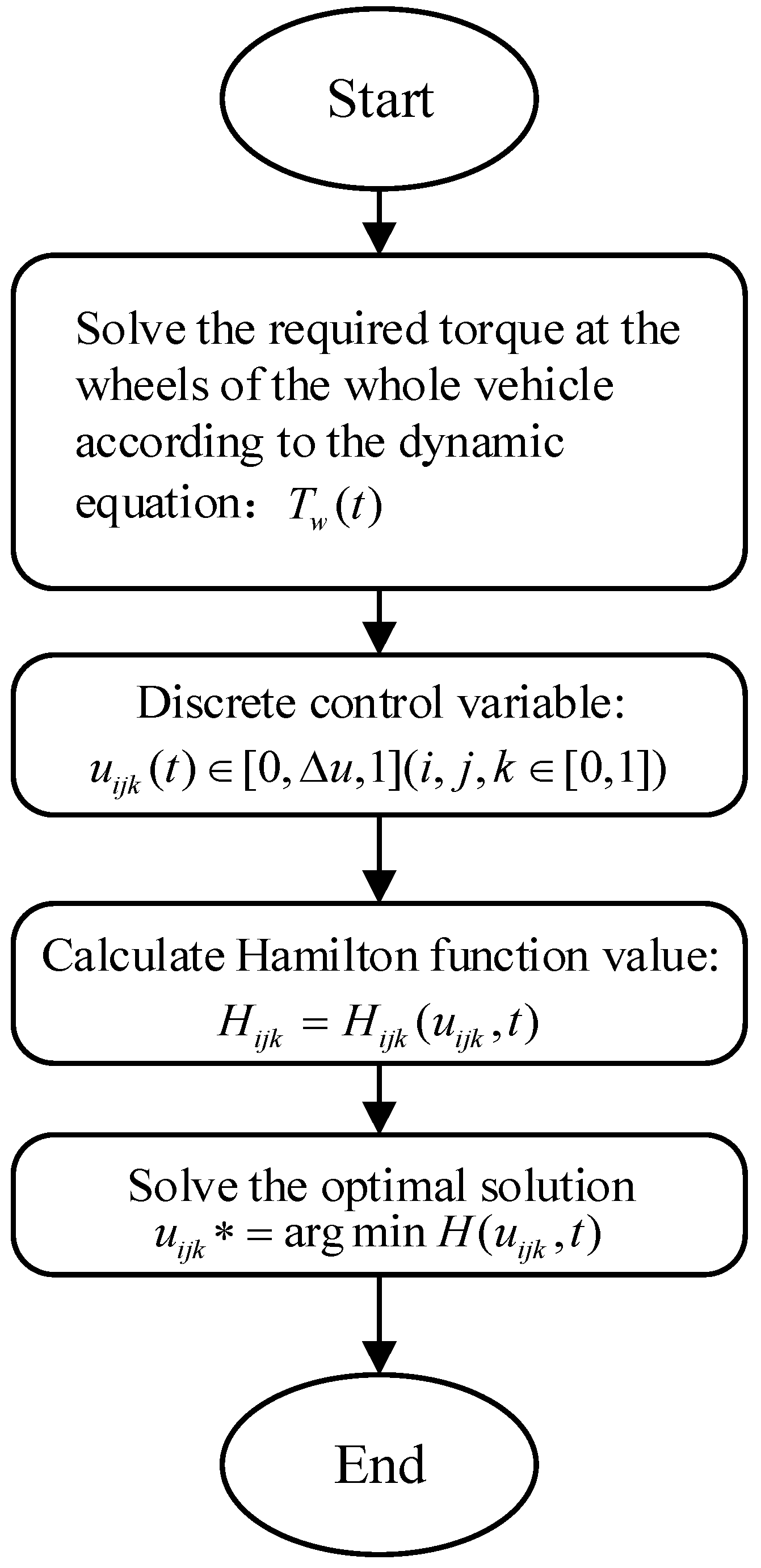
The control strategy based on the PMP adopts the cyclic iterative method to optimize the output torque of the driving torque reasonably, which can minimize the power consumption of the vehicle. The specific steps [30] are as follows.
- (1)
- The required torque at the wheels of the vehicle was calculated according to the equation of dynamics;
- (2)
- Step size is used to discretize the torque distribution coefficient within the value range;
- (3)
- For each discrete torque coefficient matrix , the value of Hamilton function corresponds to each candidate control variable, until the end of the cycle;
- (4)
- Obtain the optimal control variable.
The solution flow of PMP is shown in Figure 2.
4. BAS-PSO Optimization Algorithm
In order to speed up the optimization process of the PMP energy management strategy, the optimization algorithm is a good solution. The vehicle dynamics model is a very complex nonlinear model, which cannot be expressed by a simple transfer function or a set of simple transfer functions to solve the optimal solution. For the torque distribution control of multi-power sources in a vehicle dynamics model, it is difficult to solve multi-parameter nonlinear equations [31]. Generally, the optimal control of such models requires the use of optimization algorithms to find the optimal solution, such as particle swarm optimization algorithm, genetic algorithm, simulated annealing algorithm, etc. The previous single class of algorithms, due to its low accuracy, slow convergence rate, complex process, and other problems, cannot be applied to today’s research. To improve the operation speed of the program and avoid local optimal and premature conditions, this paper adopts a longhorn group hybrid optimization algorithm to carry out torque optimization control.
4.1. BAS-PSO
BAS is an intelligent optimization algorithm that was first proposed in 2017. Different from other bionic algorithms, it is a single search algorithm, which has the advantages of simple principle, less parameters, and less calculation. It has great advantages in dealing with low-dimensional optimization objectives [32].
The total power of the vehicle during turning is the objective function of the optimization in this paper. The fitness function can be expressed as
The BAS algorithm imitates the foraging behavior of a beetle in nature. In the process of foraging, the food will produce a special odor, which attracts the beetle to move toward the food. Before starting, the initial position of beetle and its random initial velocity will be generated randomly within the boundary of the condition. The beetle uses its two antennae to sense food smells in the air. The locations of the two antennae of longicorn are updated as follows:
where is the distance from the individual centroid to the whisker.
The concentration of odor that is perceived by the two antennae varies according to the distance between the two antennae and the food. According to the position of two antennae of beetle and , the fitness values are and . In accordance with the fitness value perceived by two antennae, the beetle advances to the side with higher fitness value at random. The location updates of the beetle can be expressed as
where is the speed of longicorn at the moment ; is the step size of the moment . In order to improve the search accuracy of Longicorn beetles in the later stage of the search and prevent longicorn beetles from missing food locations due to an excessive search step size, step attenuation coefficient is set here [33].
Through iteration after iteration, the food is finally located. However, the convergence speed of longniushu algorithm is slow and it focuses on the individual without considering the relationship between groups. Particle swarm optimization (PSO) is a global optimization algorithm, which has fast convergence speed and fully considers the influence of the group on the individual, ignoring the judgment of the individual. Therefore, this algorithm adopts a population of beetles instead of an individual beetle, which changes the speed update and position update among beetles in order to strengthen the interrelation between the groups [34]. It allows each beetle to share food location information with all beetles in the population during an individual search. Velocity and position updates can be expressed as
where is the inertia of longicorn speed, which is the influence coefficient of speed in this round on speed update in the next round; and are the individual learning factor; and are random numbers between intervals; and is the weight coefficient of the speed update.
After each iteration, the group of beetles will update the individual optimal value and the population optimal value of the current population:
Results are compared and updated with the optimal results of the last iteration. When the iteration is completed, the optimal value and the optimal solution of this optimization process will be obtained, which are the lowest turning energy loss and the optimal torque distribution coefficient of the vehicle under current conditions.
BAS-PSO is also one of the metaheuristic algorithms. At present, GA and its derivative algorithm are the most popular metaheuristic algorithms used by scholars. BAS-PSO and GA are very similar, and they are all bionic and random algorithms. According to the fitness function, both of them carry out a certain random search, and the fitness function is used to evaluate the system to obtain the optimal solution of the optimization goal. However, they are also fundamentally different. BAS-PSO does not have genetic operations such as crossover and mutation, and searches are determined based on the antennae and speed of beetle. Another important feature of BAS-PSO is memory. GA has no memory, and the previous knowledge is destroyed with the change of population. Bad results may also be retained. Compared with GA, the information-sharing mechanism of BAS-PSO is very different. In GA, chromosomes share information with each other, but crossover and mutation do not necessarily get better results. So, the movement of the whole population is relatively uniform toward the optimal region. In BAS-PSO, only the optimal individual gives information to other individuals, which is a one-way information flow. The whole search and update process follows the current optimal solution. Compared with GA, all individuals may converge to the optimal solution faster in most cases. Therefore, BAS-PSO has obvious advantages in optimization speed compared with GA.
4.2. Iteration Stop Condition
The problem described in this paper is a three-dimensional numerical optimization problem through some experimental data and the observation of the iterative process of the algorithm. The BAS-PSO algorithm has high search efficiency for low-dimensional problems. Compared with the maximum number of iterations, only a few iterations are needed to complete the search for the optimal position, and the subsequent optimization is ineffective. However, there are also some searches that find the optimal solution when they are close to the maximum number of iterations. If only the maximum number of iterations is reduced, the optimal solution will be missed. In order to reduce the time of invalid optimization without missing the optimal solution, appropriate iteration stopping conditions should be added.
The whole operation process of BAS-PSO can be shown in Figure 3 below.
Set up a counter, tolerance set , and maximum count . According to the research objective of this paper, the tolerance set and the maximum count value are taken as appropriate values, where . After the optimal fitness value is obtained in each iteration, the fitness value is compared with the optimal fitness value in the previous iteration in the process of iteration. The fitness value in the current iteration must be less than or equal to the fitness value in the last iteration. Therefore, the corresponding judgment is made for the difference between the two fitness values:
- (1)
- if , ;
- (2)
- if , ;
- (3)
- if , .
If the number of iterations does not exceed the maximum and the counter value exceeds the maximum value, the iteration cycle will jump out. The group of beetles stop searching. If the maximum number of iterations has been reached, the iteration cycle will jump out of the loop directly, and the group of beetles stop searching. Finally, the optimal position solution of this beetles search will be output.
5. Simulation Analysis
5.1. Simulation Analysis Based on BAS-PSO
BAS-PSO makes full use of the global search function of PSO and the local search ability of BAS to avoid premature optimization. It can also improve convergence speed and optimization time.
Among the BAS and PSO algorithms, the PSO algorithm has excellent global search ability to accurately find the best value in the whole region, but its local search ability is weak due to its insufficient local search accuracy. The BSO algorithm is excellent in local search ability, but it is easy to fall into local optimal in the process of search because one beetle results in weak global search ability. The BAS-PSO hybrid optimization algorithm absorbs the advantages of the two algorithms, so that it can quickly find the best value in the whole domain and avoid falling into local optimal and premature.
We will compare the search of BAS, PSO, GA, BAS-PSO, and GA-PSO in the following simulation. In order to ensure the consistency of the experiment, the initial conditions of each optimization will tend to be consistent. The optimization parameters are shown in Table 1.
As shown in Figure 4a–d, the results and operation speed of the three random algorithms are random. Both fusion algorithms will quickly converge to this optimal solution. Differences in subjects and working conditions may have an impact on the search. The computational efficiency and speed of the algorithm fluctuate to a certain extent. The BAS-PSO algorithm in Figure 4a–c can find the optimal value efficiently and quickly, while Figure 4d shows that the BAS-PSO algorithm will not quickly iterate near the optimal value but can finally find the optimal value. The adaptive fusion of the two algorithms improves the speed of the algorithm and the stability of search efficiency to a certain extent. In a few cases, the stability will be reduced, and the optimization speed will be slow. However, under the current working conditions of the research object in this paper, the search speed and efficiency of the BAS-PSO algorithm are significantly higher than other algorithms. When the appropriate iteration stops, conditions are added to the BAS-PSO algorithm.
The number of iterations of the optimization algorithm is shown in Table 2. As can be seen from Table 2, different times of invalid search time will be saved in different situations. A few of these can reduce the search time by up to 60% of the maximum number of iterations, while the general case reduces the search time by around 30%. The lowest case is when the counter has not yet reached its maximum count value and the algorithm continues to compute until the iteration terminates. The addition of an iterative stopping condition can effectively reduce the time consumed during the iterative process and speed up the optimization search of the algorithm to a certain extent.
5.2. Simulation Analysis Based on Dynamic Vehicle Model
In the TVD control of a vehicle model, the same speed and the same driving track should be maintained from the end to the beginning. As there is only a small difference between the two front wheel angles, the left front wheel angle is used as the front wheel angle in this paper for the experiment. In order to illustrate the optimal torque distribution coefficient under different turning conditions and different vehicle speeds, a series of comparative simulations of constant radius and constant vehicle speed will be carried out in this section, which will take the BAS-PSO hybrid optimization algorithm to carry out off-line optimization of the torque distribution coefficient.
For ease of presentation, the current cornering conditions are expressed in terms of the front wheel angle under equal torque distribution. The BAS-PSO hybrid optimization algorithm was used to determine the final torque distribution coefficients for the different operating conditions of the vehicle as shown in the table below.
Taking the vehicle speed of 10 km/h and the front wheel angle of 3° as an example, the evolution algebra and the change of fitness function values are shown in Figure 5. The fitness in the figure is the energy consumption of the whole vehicle (W). It can be seen from Figure 5 that the BAS-PSO hybrid optimization algorithm can be used to quickly find the optimal torque allocation ratio so as to reduce the power demand in the turning process and effectively improve the optimization speed.
It can be seen from Table 3 that at the same speed, the value of the front axle distribution coefficient increases gradually with the increase in the front wheel angle. The inner torque distribution coefficient decreases gradually. The vehicle gradually approaches the front drive, and the driving torque of the outer wheel increases gradually. From Equation (8), as the torque gradually shifts to the outside, the vehicle’s direct yaw moment gradually increases. The greater steering moment gained by the vehicle during cornering can compensate to some extent for the front wheel angle, which allows the vehicle to complete the turn with a smaller front wheel angle. The vehicle will be more energy efficient during cornering. The torque distribution coefficient matrix in the table decreases with the increase in the vehicle speed. As the speed of the vehicle increases, it will become unstable and roll over as the front wheels turn out of range during the turn. However, the TVD control is only implemented when the vehicle is in a steady state. When the vehicle does not meet the steady-state driving constraints of Equation (27) in the calculation process, the data calculation of the next set of working conditions will start. Therefore, only the torque distribution coefficient values of the vehicle in the steady state are shown in the Table 3.
The vehicle motion state and energy consumption changes before and after torque optimization distribution at the simulation speed of 40 km/h are taken as an example, as shown in Figure 6. As can be seen from Figure 6a, the vehicle gradually tends to be driven on the front axle, and the torque is shifted to the outer wheels under TVD control. In Figure 6b, the left ordinate represents the vehicle power demand, and the right ordinate represents the vehicle energy-saving ratio. It can be seen that with the increase in the front wheel angle, the difference between the vehicle power demand before and after the torque optimization allocation is gradually increasing. The energy-saving ratio before and after the torque optimization allocation is gradually increasing. In Figure 6c, the two graphs represent the front wheel angle of the vehicle before and after optimization, respectively. It can be seen that the demand of front wheel angle is reduced with the TVD control because of the compensation of direct yaw moment for front wheel angle.
Figure 7 shows the energy-saving effect of vehicle torque optimization distribution at a speed of 10–80 km/h under steady state, which is obtained through a large number of simulation optimization tests. According to the theoretical analysis in Section 2, when the vehicle speed and the front wheel angle are not large, the total energy consumption of the whole vehicle is not large and has little impact on the overall energy consumption of the vehicle. With the increase in vehicle speed and front wheel angle, the total power loss gradually increases. At this time, the vehicle obtains a certain direct yaw moment to compensate for the direct yaw moment and front wheel angle, thus reducing the energy consumption of the whole vehicle. As can be seen from Figure 7, with the increase in front wheel angle, the energy-saving ratio of TVD increases gradually. As the vehicle speed increases, the energy-saving ratio from the optimized torque distribution gradually increases. For the model described in this paper, its highest energy-saving ratio is 3.788%, corresponding to the driving condition of 80 km/h speed and front wheel angle of about 3°.
6. Conclusions
1. Through the theoretical derivation of a 7-DOF vehicle dynamics model and the analysis of the energy consumption of the whole vehicle, the impact of the TVD control on the reduction in vehicle cornering energy consumption was explained.
2. Based on the PMP, the optimal control strategy of minimum turning energy consumption torque was constructed. For vehicle cornering energy consumption, the optimization problem was simplified as “Taking vehicle speed as the state variable of the system, four-wheel torque distribution coefficient as the control variable of the system, and minimum vehicle power as the optimization objective”. The vehicle dynamics model was further analyzed, and the Hamiltonian equation was constructed to solve the optimal control variables. Aiming at the problem of a complex nonlinear vehicle dynamics model, this paper effectively solves the energy optimization problem with multiple control constraints and boundary conditions by constructing a reasonable energy management strategy.
3. The control strategy constructed based on the PMP takes the target speed and the target yaw speed as the control objectives. The torque distribution coefficients were optimized offline by BAS-PSO. Finally, the minimum torque distribution coefficient table based on the vehicle dynamics model was developed, and the optimal contribution degree of energy saving was determined for torque distribution control under different bend conditions. Simulation analysis shows that the torque optimization control can reduce the energy consumption of vehicle turning by 3.788% according to the vehicle dynamics model established in this paper. Experiments show that this paper optimizes the energy consumption when turning and achieves good results.
4. The fusion algorithm used in this paper is able to find the optimal value quickly over the whole domain in the process of optimizing the energy consumption of a vehicle, without getting stuck in a situation of premature and local optimality. The optimization algorithm will improve the optimization efficiency and search speed in different situations compared with the single optimization algorithm in a single iterative optimization. In the whole optimization process, these two aspects are more stable. When the judgment condition of an iteration stop was added, the speed can be increased by up to 60% based on the number of optimization iterations in different working conditions and about 30% in general. Through some improvements, the algorithm is optimized in terms of iteration. This part of the improvement makes the experiment save a lot of computing time.
In this paper, an off-line TVD control strategy based on PMP was established for distributed drive electric vehicles. The BAS-PSO hybrid algorithm was adopted to improve the optimization speed, and iteration stop conditions were added to shorten the iteration time of the algorithm. Aiming at the BAS-PSO algorithm, we can improve the adaptability and stability of the algorithm by improving the steps in the algorithm or adding some new things. For the optimization of vehicle energy consumption in cornering, this paper took the stability as the precondition to study and did not control the stability of the vehicle. The follow-up part can also add the control of vehicle stability to coordinate control on the basis of energy saving and make a trade-off between the two in the whole control process to achieve optimal control.
Author Contributions
Conceptualization, W.S.; methodology, W.S. and J.W.; validation, X.W. and L.L.; formal analysis, W.S. and Y.C.; writing—original draft preparation, Y.C.; writing—review and editing, W.S. and Y.C. All authors have read and agreed to the published version of the manuscript.
Funding
This research was funded by the National Natural Science Foundation of China (51875235), the State Scholarship Funding of CSC (202008320074), Industry-University-Research Cooperation Project of Jiangsu Province (BY2021227, BY2021268), the Science and Technology Project of Changzhou (CZ20210033), and the Automobile Environmental Protection Innovation Leading Plan of FAW Volkswagen and China Environmental Protection Foundation.
Institutional Review Board Statement
Not applicable.
Informed Consent Statement
Not applicable.
Data Availability Statement
Data sharing not applicable.
Conflicts of Interest
The authors declare no conflict of interest. As Junnian Wang, a co-author of this paper, is an associate EIC of Energies, he was blinded to this paper during the review, and the paper is independently handled by other editors.
Nomenclature
| TVD | Torque Vectoring Distribution |
| PMP | Pontryagin Minimum Principle |
| BAS-PSO | Beetle Antenna Search–Particle Swarm Optimization |
| 4WD | 4-Wheel-Drive |
| EV | Eclectic Vehicle |
| DP | Dynamic Programming |
| RLS | Recursive Least Square |
| YSC | Yaw Stability Control |
| EMB | Electromechanical Brake |
| GA | Genetic Algorithm |
| AEFA | Artificial Electric Field Algorithm |
| AOA | Arithmetic Optimization Algorithm |
| EO | Equilibrium Optimizer |
| GWO | Gray Wolf Optimizer |
| BA | Bat Algorithm |
| HHO | Harris Hawks Optimization |
| ACO | Ant Colony Optimization |
| IHBO | Improved Heap-Based Optimizer |
| Symbols | |
| Vehicle mass (kg) | |
| Moment of inertia of the vehicle rotating (kg·m2) | |
| Rolling resistance (N) | |
| Air resistance (N) | |
| Longitudinal velocity (km/h) | |
| Lateral velocity (km/h) | |
| Yaw velocity (rad/s) | |
| Wheelbase of the vehicle from the center of mass to the front axles (m) | |
| Wheelbase of the vehicle from the center of mass to the rear axles (m) | |
| Wheelbase of the front wheels (m) | |
| Wheelbase of the rear wheels (m) | |
| Left front wheel angle (deg) | |
| Right front wheel angle (deg) | |
| Slip angle of tire (deg) | |
| Actual left front wheel angle (deg) | |
| Actual right front wheel angle (deg) | |
| Driving force of tire (N) | |
| Side force of tire (N) | |
| Longitudinal force of tire (N) | |
| Tangential force of tire (N) | |
| Speed (km/h) | |
| Sideslip angle (deg) | |
| Rolling resistance coefficient | |
| Gravitational acceleration (m/s2) | |
| Air density (kg/m3) | |
| Windward area of the body (m2) | |
| Air resistance coefficient | |
| Driving force (N) | |
| Direct yaw moment (N·m) | |
| Longitudinal slip rate (%) | |
| Tire radius (m) | |
| Wheel speed (r/s) | |
| Wheel center speed (km/h) | |
| Longitudinal slip power loss (kW) | |
| Total power loss of the vehicle (kW) | |
| Braking torque suffered by each vehicle (N) |
References
- Ma, J.; Liu, X.D.; Chen, Y.S.; Wang, G.P.; Zhao, X.; He, Y.L.; Xu, S.W.; Zhang, K.; Zhang, Y.X. Development Status and Countermeasures of New Energy Automobile Industry and Technology in China. China J. Highw. Transp. 2018, 31, 1–19. [Google Scholar]
- Yu, Z.P.; Feng, Y.; Xiong, L. Review on Development of Dynamic Control for Distributed Drive Electric Vehicle. J. Mech. Eng. 2013, 49, 105–114. [Google Scholar] [CrossRef]
- Gruber, W.; Back, W.; Amrhein, W. Design and implementation of a wheel hub motor for an electric scooter. In Proceedings of the IEEE Vehicle Power and Propulsion Conference, Chicago, IL, USA, 6–9 September 2011; pp. 1–6. [Google Scholar]
- Xu, X.; Chen, T.; Chen, L.; Cai, Y.F.; Wang, W.J. Torque Energy Saving Optimal Allocation for Distributed Drive Electric Vehicle. China J. Highw. Transp. 2018, 31, 183–190. [Google Scholar]
- He, J.; Crolla, D.A.; Levesley, M.C. Integrated active steering and variable torque distribution control for improving vehicle handling and stability. R. SAE Trans. 2004, 113, 38–47. [Google Scholar]
- Wang, J.N.; Yang, B.; Wang, Q.N. Overview of the development of vehicle torque directional distribution drive technology. J. Mech. Eng. 2020, 56, 109–121. [Google Scholar]
- Oh, K.; Joa, E.; Lee, J.; Yun, J.; Yi, K. Yaw Stability Control of 4WD Vehicles Based on Model Predictive Torque Vectoring with Physical Constraints. Int. J. Automot. Technol. 2019, 20, 923–932. [Google Scholar] [CrossRef]
- Park, J.-Y.; Heo, S.-J.; Kang, D.-O. Development of Torque Vectoring Control Algorithm for Front Wheel Driven Dual Motor System and Evaluation of Vehicle Dynamics Performance. Int. J. Automot. Technol. 2020, 21, 1283–1291. [Google Scholar] [CrossRef]
- Meng, Q.; Zhao, T.; Qian, C. Integrated Stability Control of AFS and DYC for Electric Vehicle Based on Non-smooth Control. Int. J. Syst. Sci. 2018, 49, 1518–1528. [Google Scholar] [CrossRef]
- Chae, M.; Hyun, Y.; Yi, K. Dynamic Handling Characteristics Control of an in-Wheel-Motor Driven Electric Vehicle Based on Multiple Sliding Mode Control Approach. J. IEEE Access 2019, 7, 132448–132458. [Google Scholar] [CrossRef]
- Zhang, S.W.; Luo, Y.G.; Wang, J.M. Predictive energy management strategy for fully electric vehicles based on preceding vehicle movement. IEEE Trans. Intell. Transp. Syst. 2017, 18, 3019–3060. [Google Scholar] [CrossRef]
- Tang, Z.; Xu, X.; Jiang, X.W. Optimal torque distribution strategy for minimizing energy consumption of four-wheel independent driven electric ground vehicle. J. Appl. Sci. Eng. 2018, 21, 375–384. [Google Scholar]
- Sun, W.; Wang, J.N.; Wang, Q.N. Simulation investigation of tractive energy conservation for a cornering rear-wheel-independent-drive electric vehicle through torque vectoring. Sci. China 2018, 61, 257–272. [Google Scholar] [CrossRef]
- Wu, X.G.; Zheng, D.Y.; Wang, T.Z. Torque Optimal Allocation Strategy of All-Wheel Drive Electric Vehicle Based on Difference of Efficiency Characteristics between Axis Motors. Energies 2019, 12, 1122. [Google Scholar] [CrossRef] [Green Version]
- Wang, J.N.; Yu, T.Y.; Sun, N.N.; Fu, T.J. Torque Vectoring Control of Rear-Wheel-Independent-Drive Vehicle after Cornering Efficiency Improvement. J. Hunan Univ. (Nat. Sci.) 2020, 47, 9–17. [Google Scholar]
- Salamone, S.; Lenzo, B.; Lutzemberger, G. On the Investigation of Energy Efficient Torque Distribution Strategies through a Comprehensive Powertrain Model. J. Sustain. 2021, 13, 4549. [Google Scholar] [CrossRef]
- Liu, J.X.; Zhuang, W.C.; Zhong, H. Integrated energy-oriented lateral stability control of a four-wheel-independent-drive electric vehicle. J. Sci. China Technol. Sci. 2019, 62, 2170–2183. [Google Scholar] [CrossRef]
- Zhang, X.; Gohlich, D. Integrated Traction Control Strategy for Distributed drive electric vehicles with Improvement of Economy and Longitudinal Driving Stability. Energies 2017, 10, 126. [Google Scholar] [CrossRef] [Green Version]
- Yang, K.; Xie, L.Q.; Wang, J. The yaw stability control of rear drive all-electric independent drive-brake electric vehicle. J. Xi’an Jiaotong Univ. 2019, 53, 44–51. [Google Scholar]
- Kharrich, M.; Abualigah, L.; Kamel, S.; Abd El-Sattar, H.; Tostado-Véliz, M. An Improved Arithmetic Optimization Algorithm for design of a microgrid with energy storage system: Case study of El Kharga Oasis, Egypt. J. Energy Storage 2022, 51, 104343. [Google Scholar] [CrossRef]
- Almadhor, A.; Rauf, H.T.; Khan, M.A.; Kadry, S.; Nam, Y. A hybrid algorithm (BAPSO) for capacity configuration optimization in a distributed solar PV based microgrid. Energy Rep. 2021, 7, 7906–7912. [Google Scholar] [CrossRef]
- Kharrich, M.; Kamel, S.; Hassan, M.H.; ElSayed, S.K.; Taha, I.B.M. An Improved Heap-Based Optimizer for Optimal Design of a Hybrid Microgrid Considering Reliability and Availability Constraints. Sustainability 2021, 13, 10419. [Google Scholar] [CrossRef]
- Genta, G. Motor Vehicle Dynamics: Modeling and Simulation; World Scientific: Singapore, 1997. [Google Scholar]
- Wang, J. Steering Stability Control of Four-Wheel Motor Driven Vehicle; Beijing Institute of Technology: Beijing, China, 2015. [Google Scholar]
- Kobayashi, T.; Katsuyama, E.; Sugiura, H.; Ono, E.; Yamamoto, M. Efficient direct yaw moment control: Tyre slip power loss minimization for four-independent wheel drive vehicle. Veh. Syst. Dyn. Int. J. Veh. Mech. Mobil. 2018, 56, 719–733. [Google Scholar] [CrossRef]
- Ando, K.; Sawase, K.; Takeo, J. Analysis of tight corner braking phenomenon in full-time 4WD vehicles. JSAE Rev. 2002, 23, 83–87. [Google Scholar] [CrossRef]
- Sun, W.; Wang, Q.N.; Wang, J.N. Yaw-moment control of motorized vehicle for energy conservation during cornering. Jilin Daxue Xuebao J. Jilin Univ. 2018, 48, 11–19. [Google Scholar]
- Meng, X.; Li, Q.; Chen, W.R.; Zhang, G.R. An Energy Management Method Based on Pontryagin Minimum Principle Satisfactory Optimization for Fuel Cell Hybrid Systems. Available online: https://www.researchgate.net/publication/333035433_An_Energy_Management_Method_Based_on_Pontryagin_Minimum_Principle_Satisfactory_Optimization_for_Fuel_Cell_Hybrid_Systems (accessed on 10 January 2022).
- Gao, B.; Yan, Y.; Chu, H.; Chen, H.; Xu, N. Torque Allocation Control of Four-wheel Drive EVs Considering Energy Efficiency Optimization. Sci. China Inf. Sci. 2022, 65, 122202. [Google Scholar] [CrossRef]
- Cai, Y.; Wang, Z.W.; Zeng, Y.P.; Liu, Y.G. Research on the plug-in 4WD hybrid vehicle’s control strategy based on pontryagin’s minimum principle. Available online: http://kns.cnki.net/kcms/detail/50.1044.N.20210507.1252.003.html (accessed on 10 January 2022).
- Sun, W.; Rong, J.C.; Wang, J.N.; Zhang, W.T.; Zhou, Z.D. Research on Optimal Torque Control of Turning Energy Consumption for EVs with Motorized Wheels. Energies 2021, 14, 6947. [Google Scholar] [CrossRef]
- Jiang, X.; Li, S. BAS: Beetle Antennae Search Algorithm for Optimization Problems. Int. J. Robot. Control. 2017, 1, 1. [Google Scholar] [CrossRef]
- Jiang, X.; Shuai, L. Beetle Antennae Search without Parameter Tuning (BAS-WPT) for Multi-objective Optimization. arXiv 2017, arXiv:1711.02395. [Google Scholar] [CrossRef]
- Wang, T.; Long, Y.; Qiang, L. Beetle Swarm Optimization Algorithm: Theory and Application. arXiv 2018, arXiv:1808.00206. [Google Scholar] [CrossRef]
Figure 1.
A 7-DOF vehicle dynamic model.

Figure 2.
Solution flow of PMP.

Figure 3.
Solving process of BAS-PSO.

Figure 4.
Fitness value of the 10 km/h constant radius test: (a) 3° front wheel angle; (b) 5° front wheel angle; (c) 7° front wheel angle; (d) 9° front wheel angle.
Figure 4.
Fitness value of the 10 km/h constant radius test: (a) 3° front wheel angle; (b) 5° front wheel angle; (c) 7° front wheel angle; (d) 9° front wheel angle.

Figure 5.
Fitness value of the 10 km/h constant radius test.

Figure 6.
(a) 40 km/h, 3° front wheel angle; (b) optimized energy consumption diagram at 40 km/h; (c) optimize the distribution of front and rear wheel angles at 40 km/h.
Figure 6.
(a) 40 km/h, 3° front wheel angle; (b) optimized energy consumption diagram at 40 km/h; (c) optimize the distribution of front and rear wheel angles at 40 km/h.


Figure 7.
Energy-saving effect of optimal torque distribution.


Table 1.
Optimization parameters.
| Optimization Parameters | |||
|---|---|---|---|
| BAS-PSO | Value | GA-PSO | Value |
| Population size | 20 | Chromosome code length | 3 |
| Maximum number of iterations | 50 | Crossover probability | 0.7 |
| Initial step size | 0.8 | Mutation probability | 0.3 |
| Maximum speed of longicorn update | 0.3 | Optimal position step size of individual | 1.49445 |
| Minimum speed of longicorn update | −0.3 | Optimal position step size of group | 1.49445 |
| Learning factor | 2 | Generation amount | 50 |
| Inertia factor | 0.5 | Population size | 20 |
| Distance between two whiskers of longicorn beetle | 0.5 | Maximum speed of particle update | 1 |
| Maximum timing | 30 | Minimum speed of particle update | −1 |
Table 2.
Optimization and without optimization’s number of iterations.
| Test 1 | Test 2 | Test 3 | Test 4 | Test 5 | |
| Optimization | 20 | 24 | 28 | 32 | 36 |
| Without optimization | 50 | 50 | 50 | 50 | 50 |
| Test 6 | Test 7 | Test 8 | Test 9 | Test 10 | |
| Optimization | 50 | 27 | 41 | 30 | 34 |
| Without optimization | 50 | 50 | 50 | 50 | 50 |
Table 3.
Torque distribution coefficient.
| Front Wheel Angle (deg) | Vehicle Speed (km/h) | ||||
|---|---|---|---|---|---|
| 10 | 20 | … | 70 | 80 | |
| 1 | [0.8110, 0.4232, 0.2834] | [0.7159, 0.3791, 0.3932] | … | [0.6830, 0.3207, 0.3727] | [0.8913, 0.4125, 0.1459] |
| 3 | [0.8323, 0.4493, 0.4134] | [0.7738, 0.4625, 0.4980] | … | [0.9841, 0.2894, 0.3264] | [0.9981, 0.3559, 0.2976] |
| 5 | [0.8878, 0.4040, 0.3857] | [0.8119, 0.3804, 0.4871] | … | [1, 0.2552, -] | - |
| 7 | [0.9223, 0.4018, 0.3761] | [0.8518, 0.4024, 0.4598] | … | - | - |
| … | … | … | … | … | … |
| 27 | [1, 0.2989, -] | [1, 0.3214, -] | … | - | - |
| 29 | [1, 0.2891, -] | - | … | - | - |
Publisher’s Note: MDPI stays neutral with regard to jurisdictional claims in published maps and institutional affiliations. |
© 2022 by the authors. Licensee MDPI, Basel, Switzerland. This article is an open access article distributed under the terms and conditions of the Creative Commons Attribution (CC BY) license (https://creativecommons.org/licenses/by/4.0/).
Share and Cite
MDPI and ACS Style
Sun, W.; Chen, Y.; Wang, J.; Wang, X.; Liu, L. Research on TVD Control of Cornering Energy Consumption for Distributed Drive Electric Vehicles Based on PMP. Energies 2022, 15, 2641. https://0-doi-org.brum.beds.ac.uk/10.3390/en15072641
AMA Style
Sun W, Chen Y, Wang J, Wang X, Liu L. Research on TVD Control of Cornering Energy Consumption for Distributed Drive Electric Vehicles Based on PMP. Energies. 2022; 15(7):2641. https://0-doi-org.brum.beds.ac.uk/10.3390/en15072641
Chicago/Turabian StyleSun, Wen, Yang Chen, Junnian Wang, Xiangyu Wang, and Lili Liu. 2022. "Research on TVD Control of Cornering Energy Consumption for Distributed Drive Electric Vehicles Based on PMP" Energies 15, no. 7: 2641. https://0-doi-org.brum.beds.ac.uk/10.3390/en15072641
Note that from the first issue of 2016, this journal uses article numbers instead of page numbers. See further details here.