Periglacial Landforms and Fluid Dynamics in the Permafrost Domain: A Case from the Taz Peninsula, West Siberia

Abstract

Most of the developing oil and gas fields in Russia are located in Arctic regions and constructed on permafrost, where recent environmental changes cause multiple hazards for their infrastructure. The blowing-up of pingos, resulting in the formation of gas emission craters, is one of the disastrous processes associated both with these external changes and, likely, with deep sources of hydrocarbons. We traced the channels of fluid migration which link a gas features reservoirs with periglacial phenomena associated with such craters with the set of geophysical methods, including common depth point and shallow transient electromagnetic methods, on an area of a prospected gas field. We found correlated vertical anomalies of acoustic coherence and electrical resistivity associated with gas chimneys in the upper 500–600 m of the section. The thickness of the ice-bonded permafrost acting as a seal for fluids decreased in the chimney zone, forming 25–50 m deep pockets in the permafrost base. Three pingos out of six were located above chimneys in the study area of 200 km². Two lakes with parapets typical for craters were found. We conclude that the combination of applied methods is efficacious in terms of identifying this type of hazard and locating potentially hazardous objects in the given territory.

1. Introduction

A substantial share of proven fossil fuel resources is located in the permafrost zone. Accelerated Arctic warming and exploration increase the temperature and decrease the strength of permafrost. In addition to the expenses involved in improving the safety of exploitation, the maintenance of the infrastructure, geotechnical solutions to stabilize exogenous processes, and the clean-up of environmental damage, there are new risks associated with endogenous geological processes [1,2,3]. Among the latter, the explosive process of gas-emission crater (GEC) formation has made the greatest impact [4,5].

Since 2014, 17 GECs have been found in the north of West Siberia [6]. The process of GEC formation is still hypothesized [5,7,8,9,10,11]; however, it has distinct links with periglacial landforms which have formed by the freezing of water-containing sediments and the ones formed by the thawing of permafrost [12]. GECs are preceded by the mound-shaped landforms similar to frost mounds but which grow at a higher rate [13,14]. After their formation, GECs fill with water and within several seasons, acquire ing the traits of thermokarst lakes [15] surrounded by a parapet and an aureole of smaller ponds formed from the thawing of fragments of extruded and burst permafrost [14,16]. Regarding their tendency to expel gas and/or water, polished near-vertical walls with spherical voids ranging from centimeters to meters in diameter, intensive ebullition spots on the water surface and the pockmark-like topography of the bottoms of the lakes are all believed to affect the fluid-dynamic nature of GECs [5,6].

Pingos differ in structure, ice genesis and longevity. Pingos, which have many similarities with mounds that are the predecessors of GECs, are dome-shaped features of more than 10 m in height and more than 100 m in diameter. They are formed by the freezing of an aquifer in discontinuous permafrost (open-system pingos) or saturated sediments of taliks under former water bodies (closed-system pingos). They are formed by segregation, with the subsequent injection of water covering each frozen layer, and growth of an ice core from both intrusive and segregated ice [17]. The form, size and distribution of gas bubbles in the ice of the core were always considered a trait of the ice genesis. The connection between both pingos and thermokarst lakes and tectonic structures has been hypothesized [18,19]. However, gas or any other fluid except water has not been considered a substantial contributor to pingo growth.

Both types of pingos can accumulate methane. Firstly, taliks are relatively warm and long-lasting environments, with anaerobic conditions. There are able to deliver more than 0.03 m³ of gas per 1 m² per day to the atmosphere [20]. Secondly, freezing displaces gas in cryogenic traps [8,21]. Additional gas in open systems comes from deeper sources, as evidenced by the dominance of seeps of coalbed methane from inland water objects in sporadic or isolated permafrost zones where aquifers are more common [22]. Spatially and temporally heterogenic permafrost formation above gas-oil bearing structures has formed a complex system of gas pockets and migration channels in the Yamal and Taz peninsulas [23,24].

The size, form and quality of a pocket/channel and its connection to the source, i.e., the permafrost structure, determine the risk of the catastrophic collapse of mounds in the permafrost zone. Such pockets/channels could be a cavity in permafrost filled by pressurized gas [9], a pathway along the fractured zone around tectonic faults [11] or permafrost saturated by gas bubbles ascending through permafrost in a viscous-plastic manner [10].

The shallow transient electromagnetic method (sTEM) has proved to be good supplement to seismic tomography or it can be applied on its own to investigate features of permafrost sequences and to build models of the upper part of sections [24,25]. Ice inclusions and bands change the electrical features of deposits when compared to their thawed state, resulting in, higher values of electrical resistivity. However, differences in unfrozen water content due to interactions with the mineral particles of sediments, temperature, and salinity result in a wide range of reasonable interpretations in terms of electrical properties [26].

STEM was used to determine permafrost thickness, as well as the distribution of taliks and gas migration channels through frozen ground and to study the links between periglacial landforms and anomalies of permafrost structures traced down to the base at a depth of 400 m using 3D acoustic and electrical resistivity models. Anomalies were supported by the presence of fluid. We suggest the verified combination of methods to determine new endogenic hazards in Arctic regions [27,28,29].

2. Materials and Methods

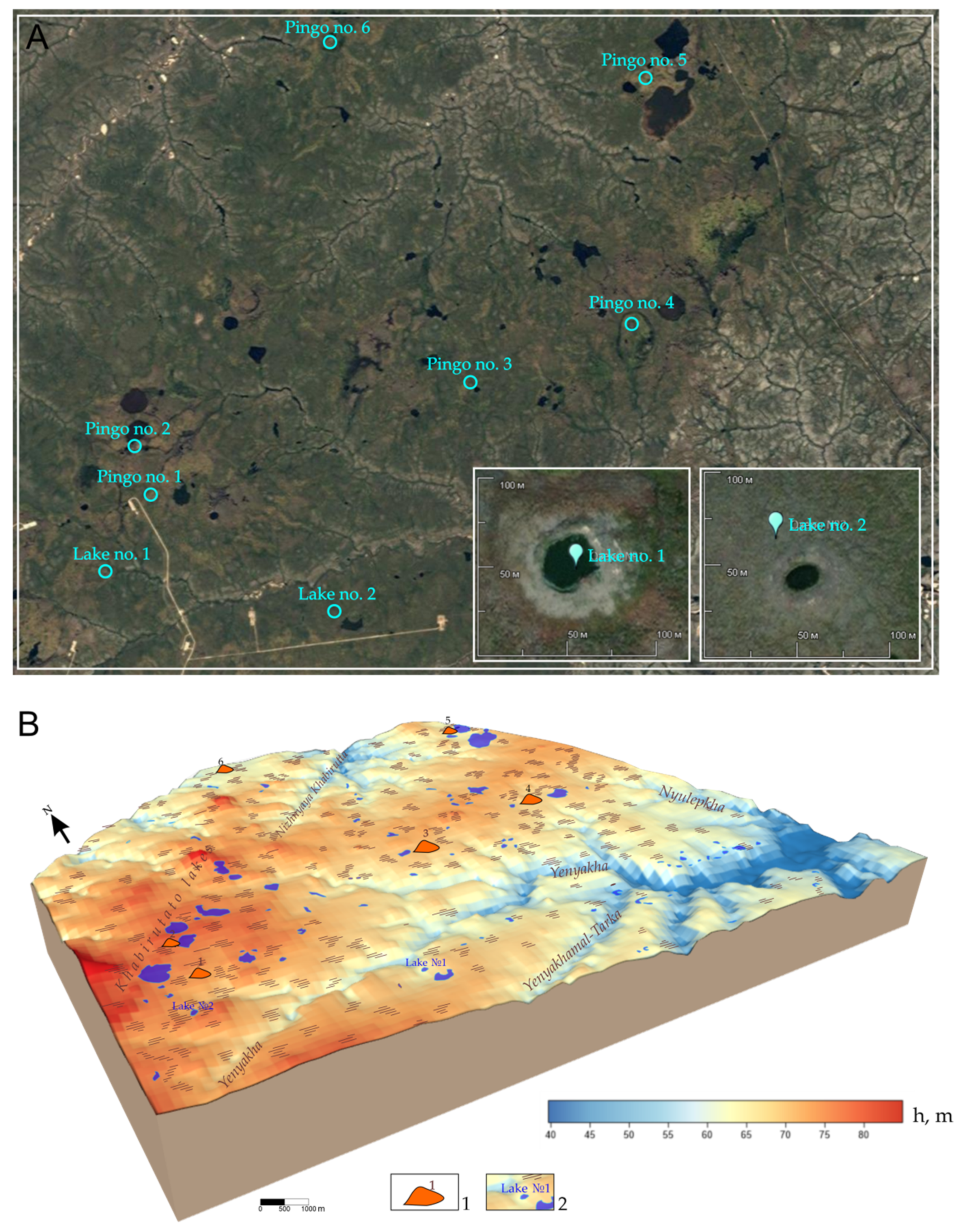
2.1. Study Area

We studied the upper 500 m of a section of an oil and gas field on the Nadym and Pur watershed presented by a 40–80 m high plain of the Kazantsevo marine transgression (Marine Isotope Stage 5) eroded by rivers and springs and with abundant lakes (Figure 1).

The study area lies in the north of the region of the two-layer permafrost sequences consisting of a lower relict Pleistocene permafrost and an upper epigenetic Holocene permafrost intervened by the hydrothermal talik [30]. The depth of early Holocene thawing of permafrost ranged from 70–90 m in forest tundra to 120–150 m in northern taiga. Climate cooling in the Late Holocene caused new freezing of the sediments and the formation of the upper permafrost layer. The talik between the layers is thinning northwards from the first ten meters of saturated sediments.

The periglacial processes of the study area are associated with seasonal freezing/thawing, frost heaving and frost cracking. Thermokarst is manifested in numerous lakes of various forms and sizes and vast alases.

Pingos reaching heights of 15–20 m and diameters of 300 m, surrounded by piedmont glaciers of 1–2 m in height, are widely distributed on the Kazantsevo marine plain (Figure 2). They have a massive ice or massive-agglomerate cryostructure in their core. Several the pingos in the study area possess dilation cracks, marking their continuous growth, and several have already collapsed, with fissures and craters formed by the initiation of thermokarst. Pingos are organized in groups or lines on the territories of the Pestsovoe and the En-Yakhinskoe fields. However, they are more sparsely distributed in the neighboring north of the Urengoy field. Other frost heaving forms include palsas and peat plateaus, which occur in alases where peat deposits are more extensive.

Gas phase extracted from pingo ice contained up to 8% vol. of methane [19] and 4% vol. of hydrogen, which falls into range of concentration of explosion danger. Here we report on several other frost mounds containing and missing gas accumulations within the upper section [23] in relation to their structure obtained from geophysical studies. Gas-bearing ice crystallites were found below the base of another pingo, which is an indicator of crystal growth in supersaturated environment [31]. Structure of permafrost sequences within fluid migration zone have shearing deformations not only in the pingo ice or the ice-rich core but also tens of meters below.

The lakes of the study area differ in color, with some of them being brown and rich in organic matter, while others are blue and hold clear water. The transparent water in the blue lakes in some cases exposes the pockmark-like relief of the lake bottoms. The color of the lakes, the specific bottom topography and increased concentration of methane and helium have for a long time encouraged the belief that there is a connection between lake color and fluid migration [32]. However, years of studies led the same authors to conclusions that bacterial methanogenesis drives the ebullition events which cause pockmarks to occur and that sulfur ions entering the biogeochemical cycles of lakes from marine deposits cause the blue color [33]. So, only reliable geophysical data can clearly determine whether there are fluid contributions to lakes of different colors.

Frost cracking is widespread in the study area, forming a polygonal pattern at all geomorphological levels.

2.2. Shallow Transient Electromagnetic Data

The shallow transient electromagnetic method (sTEM) is one of the most efficacious in studies of the upper part of the section [34,35]. The survey is performed using a primary electromagnetic EM field, which is generated by switching the transmitter current off in a controlled way and registering the secondary EM field decay signals. The rate of decay is proportionate to the electric conductivity of sediments. The EM field penetrates into the geological section according to the induction principle, which is the physical basis of the of the method, so that using ungrounded transmitter and receiver loops allows for surveying across high resistivity layers which are usually impermeable to other methods employing direct currents. Another advantage of this method is the lack of grounding, which allows surveying all year round, regardless of the frozen/thawed state of soils. The sounding depth is controlled by decay duration due to the skin effect [36,37]. STEM template with a rectangular transmitter loop of 100 × 100 m and a receiver loop of 10 × 10 m allowed us to survey the section of 500–600 m in conditions of hydrocarbon fields of West Siberia [35]. The current of up to 30 Amp generated in a transmitter loop induced one coaxial and two offset receivers.

Field electromagnetic records characterizing the electric properties of the section, processed using specific procedures of noise attenuation, resulted in the depth profiles of the electromotive force, apparent resistivity and apparent conductivity of sediments [34]. The analysis of each section was performed by solving the 1D inverse geophysical problem for floating structures, i.e., varying levels of specific electrical resistivity and thickness of layers [26]. Modeling was performed using distributed computing technology, which significantly decreased the time of analysis. The results of an inverse modeling of 6600 sTEM stations for 200 km² is presented in this study. Each geoelectrical model contains 15–16 layers of increasing thickness with depth. They have been combined into a single 3D electrical resistivity cube, corrected for topography using a digital elevation model and validated against lithology using drilling data in order to correlate geolectrical layers and geology.

We used the data from the borehole no 221 located within the study area (Figure 3), the unified regional stratigraphic schemes [38] and scrupulous description of the sediment structure based on drilling data Volkova [39] for the geological interpretation of geophysical data.

2.3. Common Depth Point Seismic Reflection Data

We employed data from a recent 3D common depth point (CDP) seismic exploration of the whole study area. A cube of the seismic coherence records was analyzed to find weak zones in altitudes ranging from −150 to −600 m a.s.l. The discontinuity of reflections, column-shaped forms and amplitude attenuation are specific features indicative of the migration of deep fluids in seismic data [40]. The OpendTect 6.2 (dGB Earth Sciences, Enschede, The Netherlands) software package delivers an instrument “chimney” to calculate the vertical gas migration channels (chimneys). The instrument combines attributes of curvature, coherency and dispersion through a neural network. We used analogous algorithm in different analytical complex developed for Paradigm (Emerson E&P Software, Houston, TX, USA).

3. Results

3.1. Structure of the Upper Part of the Section Based on Electromagnetic Survey

Two layers of permafrost typical for the southern region of West Siberia [30] were sufficiently recognized, Figure 3. The layer of epigenetic permafrost stretching from the surface down to 80–100 m depth had a resistivity ranging from 100 to 2000 Ω m due to a high ice content, 40–50%, and a low temperature, −4 to −5 °C. It was underlain by a layer of permafrost with an ice content of about 10 %, a temperature ca. −2 °C down to the total depth of −80–100 m. Electrical resistivity varied, but gradually fell from 500 to 20 Ω m. Below, in the interval of absolute depths of −100–120 m, there was a 20 m thick lateral talik which had an electrical resistivity of 20 Ω m. Deeper down, there was a 200 m thick layer of relic permafrost with a resistivity of 25–40 Ω m, with the base traced at the range of depths from −120 to −320 m. It had a temperature of −0.6 °C and was composed by cryotic ground without ice inclusions.

Vertical anomalies in the EM field percolating the horizontal layers of sediments could be traced on geoelectrical sections in the interval from −25 down to below −400 m below sea level. They had either a low of 5–10 Ω m or a high electrical resistivity of 40–100 Ω m compared to the enclosing strata (see Figure 3). Vertical anomalies with relatively low resistivity were traced within permafrost intervals. Above these anomalies, the thickness of epigenetic permafrost changed by 30–40% compared to the background, Figure 4.

The average resistivity and thickness of the modern permafrost tended to follow the topography of the Cenomanian reservoir, which formed a northeasterly oriented slight arc within the study area, Figure 5.

3.2. Vertical Anomalies in the Common Depth Point Cube (3D CDP)

Superimposed 3D CDP and sTEM data revealed a correlation between the vertical anomalies in the seismic section. The main features of the anomalies in the CDP data were the loss of coherence along the vertical structures percolating the sediments. They formed low-velocity cylindrical zones in the slice which represent chimneys. These initiate at the level of the Cenomanian and Jurassic reservoirs and continue in Quaternary sediments (Figure 6). In several cases, they were found below the periglacial landforms (Figure 7).

3.3. Geophysical Anomalies and Cryogenic Features

We found eight cryogenic landforms which could be associated with structures typical for gas emission craters (GECs) evolution [5,16]. These six frost mounds look like “mounds predecessors” [16] and two round lakes surrounded with parapets (Figure 1) were studied in detail. In the following description readers are referred to Figure 7 and Figure 8 for graphical representation of the geophysical data and Table with characteristics of frost mounds (

Table 1. Basic characteristics of the pingos detailed in our study. Data on altitude and diameters measured perpendicularly through the top (highest point) of the pingos are taken from ArcticDEM [41]. Form factor is the ratio of the longer diameter to the shorter.

Pingo No.	Landscape	Diameters, m	Form Factor	Altitude, m	Thickness of Epigenetic Permafrost, m
1	Kazantsevo marine plain	79.19/112.7	1.4	64	80
2	Kazantsevo marine plain	102.86/99.36	1.0	62	50
3	Alas	31.52/18.96	1.7	53	60
4	Alas	185.13/167.93	1.1	61	25
5	Alas	108.26/95.20	1.1	56	110
6	Alas	282.55/231.07	1.2	50	100

).

We did not find any significant deviations in the structure of permafrost nearby to Pingo no. 1, as interpreted from sTEM and 3D CDP data. No vertical anomalies were identified for this pingo (Figure 8A). This mound was located on the highest point of the watershed and had a slightly elongated form. Specific resistivity nearby to this pingo monotonously changed from 150 to 180 Ω m.

Pingo no. 2 was located near the lake on the high watershed. Like most of the pingos under study, it had circular shape (form factor of lower than 1.2). An anomalously low electrical resistivity was found down towards the bottom of the permafrost directly below the pingo (Figure 8B). The anomalous decrease in coherence of the seismic record at a depth ca. −500 m on the time cross section evidences the excessively fissured zone. A similar zone was found on the coherence slice at −300 m. The pingo was located within the zone with a slightly decreased resistivity of 100 Ω m.

The smallest Pingo no. 3 was also located by the lake within the isometric zone with an anomalous decrease in resistivity of 60–100 Ω m. It had a prominent linear structure typical of a palsa. The thickness of permafrost below it was also decreased, despite the fact that there were no anomalous structures in terms of either electric or seismic sections.

Pingo no. 4 had the most sophisticated structure. It was located within Alas. The sediments below had anomalously low levels of electric resistivity down to the bottom of the permafrost. The anomalous zone formed circle with an electric resistivity of 50–80 Ω m around the pingo (Figure 8C). A vertical anomaly of coherence was recognized on the 3D CDP. The slice at the level of Upper Cretaceous deposits pointed to a circular anomalous zone (Figure 9).

Pingo no. 5 was located in proximity to a large lake on a flooded watershed, in the zone of a highly-specific resistivity of sediments of 120–160 Ω m. However, an isometric anomaly of 50–80 Ω m passing through the Upper Cretaceous deposits was mapped to the south-east of the pingo (Figure 8D). The geoelectric section also evidences that the pingo was located away from the anomaly. In this case, no anomalies of coherence were found on the 3D CDP section.

Pingo no. 6, located in Alas in the north of the study area, lay in the zone of an electric resistivity of sediments of 60–80 Ω m. The local increase in the thickness of epigenetic permafrost was located above the vertical zone of low resistivity deposits, as in Pingo no. 3. There are no anomalies of coherence in this case.

There were isometric anomalies in the geoelectrical structure of sediments around Lakes no. 1 and no. 2, with a lateral resistivity of 60–100 Ω m. The thickness of epigenetic permafrost was decreased and there was an anomalously high electrical resistivity of sediments below the Lake no. 1. There was an anomalous coherence of the seismic record, evidencing the extensively fissured zone below the lake. Lake no. 2, which was significantly smaller than the Lake no. 1, had a smaller vertical anomaly of increased resistivity and permafrost thickness.

4. Discussion

4.1. Structure of Gas Reservoir Controls Thickness of Epigenetic Permafrost

A footprint of the arched structure of the cover of the Cenomanian reservoir was found in all of the covering layers of sediments. The effect of the gas reservoir could also be traced in the increased thickness of the modern permafrost (see Figure 5A,B). The arched structure is not only a classical trap for gaseous fluids, but also the zone of increased stresses, which could be released by fracturing, resulting in the leakage of the fluid. It is typical for the region of study that permafrost has begun to form above leaking gas bearing structures due to adiabatic cooling [7,42]. The process has lasted for thousands of years, forming thicker permafrost in the areas of more intensive fluid migration. Growth of the isolated permafrost coalesced into continuous massive, which was able to act as a trap on the way of the fluid migration, even above faults [43]. This process has forced fluids to accumulate in reservoirs below and within permafrost and redirects the migration flows. The irregularities of the base of epigenetic permafrost follow, among other factors, the heat flow associated with the fluid flow [18].

4.2. Gas Migration Channels Are Traced in the Upper Part of the Section

We treated the sub-vertical and inclined anomalies in the electromagnetic and seismic records as the migration channels of the fluids, where hydrocarbons from Cenomanian and Jurassic reservoirs rise up to the upper part of the section [44]. The channels could be traced as “chimneys” of low coherence on 3D CDP in the range of depths from −600 to −300 m, which continue with either high or low electric resistivity in the upper part of the section.

Low resistivity within permafrost is associated with heat and mass transfer via the fluid disturbing the temperature, unfrozen water and gas content. Around Lakes no. 1, 2 and Pingos no. 2, 4, which are located in proximity of the lakes or within alases, the electrical resistivity formed isometric anomalies of below 100 Ω·m compared to the background 140–160 Ω·m. The thickness of epigenetic permafrost also decreased to 50–75 m compared to the average 140–160 m on the study area. Both factors allow us to associate these low resistivity zones with open taliks, which exist or existed below the lakes. Taliks are more easily penetrable by fluids, providing flow up to the surface, which was confirmed by thermokarst lakes in different parts of the Arctic and with boreholes disclosing lateral taliks [22,23]. Fluids are likely able to penetrate through or destruct impermeable layers of clays/silts on the bottom of lakes and thin and warm permafrost in the bottoms of alases [4,5,9].

4.3. Certain Periglacial Landforms Are Located Close to Fluid Migration Channels in Some Cases

Low resistivity anomalies do not only spread in association with periglacial landforms in the study area and, vice versa, not all periglacial landforms are associated with fluid migration channels. Nevertheless, seismic anomalies were found under three pingos out of six and two pre-selected lakes out of two. They were connected to electrical resistivity anomalies.

In case of Pingos no. 2 and 4, with anomalously low resistivity sediments forming pockets in permafrost above the “chimneys” indicated on seismic records, we have clear evidence of the migration of fluids from the Upper Creataceous gas-bearing structure. This is supported by the borehole PCV-7/17 [23] near the top of the frost mound, which disclosed permafrost with a high concentration of methane, 2.5 g m⁻³, pressurized aquifer and weak gas show with δ¹³C(CH₄) = −64‰, pointing at a mixture of biotic and abiotic gases. The fluid migration channels in permafrost likely continue to the surface or intrapermafrost accumulations at a scale which is not detectable by the resolution of our methods.

The high resistivity and increased thickness of modern permafrost below Lake no. 2 may be associated with the more dispersed composition of Quaternary sediments compared to its surroundings or another reason listed in a numbered list below. In the cases of Pingos no. 3 and 6 and, to a lesser degree, Pingo no. 1, high resistivity may be associated with:

• A low migration rate due to seismic records having only very weak or no “chimneys”;
• Periglacial landforms, which were formed without the contribution of fluid migration;
• The buildup of ice-rich permafrost during the terminal stage of the fluid migration process because of the closure of the channel, colder temperatures or the higher freezing temperature of the fluid compared to that creating the pockets.

For Pingo no. 5, we believe the migration channel has changed direction due to the formation of the lake talik nearby, which is supported by a pocket-like permafrost bottom. Alternatively, it is due to an inclined thin undetectable migration channel from the pocket to the frost mound. Borehole PCV-8/17 [23] disclosed a pressurized aquifer and a high concentration of methane in permafrost, 2.4 g m⁻³, which could have resulted from accumulations in permafrost fed by the fluid flow which took place in the past or present continue. This could be a case in which periglacial landforms result from complex endogenous and exogenous processes.

For Lake no. 1, the borehole PCV-3/17 [23] disclosed buried soil under the sands on the surface composing the parapet, which supports the notion that it is a GEC. A low concentration of methane in the sediments of the lake shore, less than 0.1 g m⁻³, and positive anomalies in terms of permafrost thickness confirm that this object is either not filled by a migration channel anymore or that migration takes place into the lake through thin inclined channels from the pocket-like structure below.

We may speculate an evolutionary sequence for all of our cases. Given that the low resistivity zone usually surrounds taliks and is reflected in thickness of permafrost, Pingo no. 2, located on the edge of the anomalously low zone, is a young open-system pingo formed by the inflow of migration gases and requires further tracing in terms of the rate of growth.

Pingo no. 4 is a mature system fed by hydrocarbons from below and is composed of anomalously low resistivity sediments, which makes it susceptible for blow-up if the borehole did not release enough pressure. Pingo no. 3 is at the terminal stage, when a record-low thickness of permafrost is formed by the freezing of a talik, possibly due to the termination of fluid flow. Lake no. 1 is at the post-terminal stage, when thick permafrost closes up the migration channel after the release of the fluid mass.

We believe Pingos no. 2, 4 and 5 are interesting objects to track further, as they could offer further evidence of fluid dynamics in the near future.

5. Conclusions

We have demonstrated the necessity for the more detailed study of periglacial landforms which, in some cases, represent potential endogenous hazards for oil and gas exploration, production and infrastructure exploitation. Conventional CDP seismic surveys cannot be applied in the study of the upper part of the section (70–400 m), and here is where the shallow transient electromagnetic method (sTEM) could help in the building of a model of the upper 500–600 m, including the base of permafrost, taliks and cryotic grounds.

A set of methods was used for the first time to investigate the connectivity of periglacial landforms to fluid migration channels characterized either as anomalously low, 5–10 Ω m, or high, 40–100 Ω m, in terms of electrical resistivity. These anomalies were found below three out of six pingos with high gas contents in the ice core and frozen sediments, and two thermokarst lakes possessing parapets typical for gas emission craters.

We see the necessity to continue the study of such endogenous hazards by looking at the most effective set of methods to detect channels and the activity of fluid migration.

References

1. Romanovsky, V.; Isaksen, K.; Drozdov, D.; Anisimov, O.; Instanes, A.; Leibman, M.; McGuire, A.D.; Shiklomanov, N.; Smith, S.; Walker, D.; et al. Changing Permafrost and its Impacts. In Snow, Water, Ice and Permafrost in the Arctic (SWIPA); Arctic Monitoring and Assessment Programme: Oslo, Norway, 2017; pp. 65–102. [Google Scholar]
2. Meredith, M.; Sommerkorn, M.; Cassotta, S.; Derksen, C.; Ekaykin, A.; Hollowed, A.; Kofinas, G.; Mackintosh, A.; Mathias Costa Muelbert, M.; Melbourne-Thomas, J.; et al. Polar regions. In Special Report on the Ocean and Cryosphere in a Changing Climate (SROCC); Pörtner, H.-O., Roberts, D.C., Masson-Delmotte, V., Zhai, P., Tignor, M., Poloczanska, E., Mintenbeck, K., Nicolai, M., Okem, A., Petzold, J., et al., Eds.; WMO: Geneva, Switzerland; UNEP: Geneva, Switzerland, 2019; p. 173. [Google Scholar]
3. Rajendran, S.; Sadooni, F.N.; Al-Kuwari, H.A.-S.; Oleg, A.; Govil, H.; Nasir, S.; Vethamony, P. Monitoring oil spill in Norilsk, Russia using satellite data. Sci. Rep. 2021, 11, 3817. [Google Scholar] [CrossRef]
4. Leibman, M.O.; Kizyakov, A.I.; Plekhanov, A.V.; Streletskaya, I.D. New permafrost feature—deep crater in Central Yamal (West Siberia, Russia) as a response to local climate fluctuations. Geogr. Environ. Sustain. 2014, 7, 68–80. [Google Scholar] [CrossRef]
5. Bogoyavlensky, V. Gas blowouts on the Yamal and Gydan Peninsulas. GEO ExPro 2015, 12, 74–80. [Google Scholar]
6. Bogoyavlensky, V.; Bogoyavlensky, I.; Nikonov, R.; Kargina, T.; Chuvilin, E.; Bukhanov, B.; Umnikov, A. New Catastrophic Gas Blowout and Giant Crater on the Yamal Peninsula in 2020: Results of the Expedition and Data Processing. Geosciences 2021, 11, 71. [Google Scholar] [CrossRef]
7. Badu, Y.B. Gas shows and the nature of cryolithogenesis in marine sediments of the Yamal Peninsula. Kriosf. Zemli 2017, 21, 36–45. [Google Scholar] [CrossRef]
8. Kraev, G.; Schulze, E.-D.; Yurova, A.; Kholodov, A.; Chuvilin, E.; Rivkina, E. Cryogenic displacement and accumulation of biogenic methane in frozen soils. Atmosphere 2017, 8, 105. [Google Scholar] [CrossRef] [Green Version]
9. Buldovicz, S.N.; Khilimonyuk, V.Z.; Bychkov, A.Y.; Ospennikov, E.N.; Vorobyev, S.A.; Gunar, A.Y.; Gorshkov, E.I.; Chuvilin, E.M.; Cherbunina, M.Y.; Kotov, P.I.; et al. Cryovolcanism on the Earth: Origin of a spectacular crater in the Yamal Peninsula (Russia). Sci. Rep. 2018, 8, 13534. [Google Scholar] [CrossRef]
10. Khimenkov, A.N.; Sergeev, D.O.; Vlasov, A.N.; Volkov-Bogorodsky, D.B.; Tipenko, G.S.; Merzlyakov, V.P.; Stanilovskaya, Y.V. Explosive Processes in Permafrost Areas—New Type of Geocryological Hazard. In Heat-Mass Transfer and Geodynamics of the Lithosphere; Svalova, V., Ed.; Springer: Berlin/Heidelberg, Germany, 2021; pp. 83–99. [Google Scholar] [CrossRef]
11. Chuvilin, E.; Sokolova, N.; Davletshina, D.; Bukhanov, B.; Stanilovskaya, J.; Badetz, C.; Spasennykh, M. Conceptual Models of Gas Accumulation in the Shallow Permafrost of Northern West Siberia and Conditions for Explosive Gas Emissions. Geosciences 2020, 10, 195. [Google Scholar] [CrossRef]
12. Badu, Y.B.; Nikitin, K.A. Pingo within the gas-bearing structures, Northern part of West Siberia. Kriosf. Zemli 2020, 24, 17–26. [Google Scholar] [CrossRef]
13. Kizyakov, A.; Leibman, M.; Zimin, M.; Sonyushkin, A.; Dvornikov, Y.; Khomutov, A.; Dhont, D.; Cauquil, E.; Pushkarev, V.; Stanilovskaya, Y. Gas Emission Craters and Mound-Predecessors in the North of West Siberia, Similarities and Differences. Remote Sens. 2020, 12, 2182. [Google Scholar] [CrossRef]
14. Zolkos, S.; Fiske, G.; Windholz, T.; Duran, G.; Yang, Z.; Olenchenko, V.; Faguet, A.; Natali, S.M. Detecting and Mapping Gas Emission Craters on the Yamal and Gydan Peninsulas, Western Siberia. Geosciences 2021, 11, 21. [Google Scholar] [CrossRef]
15. Dvornikov, Y.A.; Leibman, M.O.; Khomutov, A.V.; Kizyakov, A.I.; Semenov, P.; Bussmann, I.; Babkin, E.M.; Heim, B.; Portnov, A.; Babkina, E.A.; et al. Gas-emission craters of the Yamal and Gydan peninsulas: A proposed mechanism for lake genesis and development of permafrost landscapes. Permafr. Periglac. Processes 2019, 30, 146–162. [Google Scholar] [CrossRef] [Green Version]
16. Kizyakov, A.; Khomutov, A.; Zimin, M.; Khairullin, R.; Babkina, E.; Dvornikov, Y.; Leibman, M. Microrelief Associated with Gas Emission Craters: Remote-Sensing and Field-Based Study. Remote Sens. 2018, 10, 677. [Google Scholar] [CrossRef] [Green Version]
17. French, H.M. The Periglacial Environment, 3rd ed.; John Wiley & Sons Ltd.: Chichester, UK, 2007; p. 458. [Google Scholar] [CrossRef] [Green Version]
18. Romanovskii, N.N. Osnovy Kriogeneza Litosfery (Fundamentals of the Cryogenesis of Litosphere); Izd-vo MGU: Moscow, Russia, 1993; p. 334. [Google Scholar]
19. Nezhdanov, A.A.; Novopavshin, V.F.; Ogibenin, V.V. Gryazevoi vulkanizm na severe Zapadnoi Sibiri (Mud volcanism in the north of West Siberia). In Sbornik Nauchnykh Trudov OOO “TyumenNIIgiprogaz” (Proceedings of LLC TyumenNIIgiprogas); Maslov, V.N., Gagarin, M.N., Laperdin, A.N., Marinenkov, D.V., Merkushev, M.I., Nesterenko, A.N., Ogibenin, V.V., Skrylev, S.A., Shtol’, V.F., Eds.; Flat: Tyumen, Russia, 2011; pp. 73–79. [Google Scholar]
20. Walter, K.M.; Zimov, S.A.; Chanton, J.P.; Verbyla, D.; Chapin, F.S. Methane bubbling from Siberian thaw lakes as a positive feedback to climate warming. Nature 2006, 443, 71–75. [Google Scholar] [CrossRef]
21. Yakushev, V.S.; Chuvilin, E.M. Natural gas and gas hydrate accumulations within permafrost in Russia. Cold Reg. Sci. Technol. 2000, 31, 189–197. [Google Scholar] [CrossRef]
22. Walter Anthony, K.M.; Anthony, P.; Grosse, G.; Chanton, J. Geologic methane seeps along boundaries of Arctic permafrost thaw and melting glaciers. Nat. Geosci. 2012, 5, 419–426. [Google Scholar] [CrossRef]
23. Kraev, G.; Rivkina, E.; Vishnivetskaya, T.; Belonosov, A.; van Huissteden, J.; Kholodov, A.; Smirnov, A.; Kudryavtsev, A.; Teshebaeva, K.; Zamolodchikov, D. Methane in gas shows from boreholes in epigenetic permafrost of Siberian Arctic. Geosciences 2019, 9, 67. [Google Scholar] [CrossRef] [Green Version]
24. Buddo, I.V.; Misurkeeva, N.V.; Shelohov, I.A.; Agafonov, Y.A.; Smirnov, A.S.; Zharikov, M.G.; Kulinchenko, A.S. Experience of 3D transient electromagnetics application for shallow and hydrocarbon exploration within Western Siberia. In Proceedings of the 79th EAGE Conference & Exhibition, Paris, France, 12–15 June 2017. [Google Scholar]
25. Seminskiy, I.K.; Murzina, E.V.; Misurkeeva, N.V.; Sharlov, M.V.; Buddo, I.V.; Shelohov, I.A.; Smirnov, A.S. Dependence of pingo placement and induction-induced polarization anomalies in the Arctic zone. In Proceedings of the GeoBaikal 2020, Irkutsk, Russia, 5–9 October 2020. [Google Scholar]
26. Pospeev, A.V.; Buddo, I.V.; Agafonov, Y.A.; Sharlov, M.V.; Kompaniets, S.V.; Tokareva, O.V.; Misyurkeeva, N.V.; Gomul’skii, V.V.; Surov, L.V.; Il’in, A.I.; et al. Sovremennaya Prakticheskaya Elektrorazvedka (Modern Applied Electroprospecting); Gladkochub, D.P., Ed.; Geo: Novosibirsk, Russia, 2018; p. 231. [Google Scholar]
27. Misiurkeeva, N.V.; Buddo, I.V.; Shelohov, I.A.; Vak, A.G. New data on fluid dynamic processes in the Arctic zone of Western Siberia based on the results of TEM, STEM electromagnetic studies and seismic CDP studies. In Proceedings of the Tyumen 2019, Tyumen, Russia, 25–29 March 2019. [Google Scholar]
28. Misurkeeva, N.V.; Buddo, I.V.; Smirnov, A.S.; Shelokhov, I.A. Shallow transient electromagnetic method application to study the Yamal Peninsula permafrost zone. In Proceedings of the Geomodel 2020, Gelendzhik, Russia, 7–11 September 2020. [Google Scholar]
29. Misurkeeva, N.V.; Buddo, I.V.; Shelokhov, I.A.; Smirnov, A.S.; Agafonov, Y.A. Permafrost rocks structure within the north of Western Siberia from modern geophysical studies. Energies 2022, 15, 1816. [Google Scholar]
30. Geokriologiya SSSR. Zapadnaya Sibir’ (Geocryology of the USSR. The West Siberia); Ershov, E.D., Ed.; Nedra: Moscow, Russia, 1989; p. 454. [Google Scholar]
31. Kurchatova, A.; Rogov, V.; Taratunina, N. Geochemical Anomalies of Frozen Ground due to Hydrocarbon Migration in West Siberian Cryolithozone. Geosciences 2018, 8, 430. [Google Scholar] [CrossRef] [Green Version]
32. Kruglikov, N.M.; Kuzin, I.L. Vykhody Glubinnogo Gaza Na Urengoiskom Mestorozhdenii (Deep Gas Shows in Urengoy Field); Trudy Zapadno-Sibirskogo Nauchno-issledovatel’skogo Geologorazvedochnogo Neftyanogo Instituta: Tyumen, Russia, 1973; pp. 96–106. [Google Scholar]
33. Kuzin, I.L. Golubye ozera oblastei gumidnogo klimata (Blue lakes of the humic climate regions). Izv. Rus. Geogr. Obs. 2001, 133, 44–57. [Google Scholar]
34. Sharlov, M.V.; Buddo, I.V.; Misyurkeeva, N.V.; Shelokhov, I.A.; Agafonov, Y.A. Transient electromagnetic surveys for high resolution near-surface exploration: Basics and case studies. First Break 2017, 35, 63–71. [Google Scholar] [CrossRef]
35. Rybalchenko, V.V.; Trusov, A.I.; Buddo, I.V.; Abramovich, A.V.; Smirnov, A.S.; Misyurkeeva, N.V.; Shelokhov, I.A.; Otsimik, A.A.; Agafonov, Y.A.; Gorlov, I.V.; et al. Integrated auxiliary studies at the stages of petroleum field prospection and development: From permafrost mapping to groundwater exploration for drilling and operation. Gazov. Promyshl. 2020, 807, 68–76. [Google Scholar]
36. Kaufman, A.A.; Morozova, G.M. Teoreticheskie Osnovy Metoda Zondirovanii Stanovleniem Polya V Blizhnei Zone (Basics of the Shallow Transient Electromagnetic Method); Nauka: Novosibirsk, Russia, 1970; p. 123. [Google Scholar]
37. Reynolds, J.M. An Introduction to Applied and Environmental Geophysics, 2nd ed.; John Wiley & Sons, Ltd.: Chichester, UK, 2011; p. 696. [Google Scholar]
38. Gurari, F.G.; Volkova, V.S.; Babushkin, A.E.; Golovina, A.G.; Nikitin, V.P.; Nekrasov, A.I.; Kriventsov, A.V.; Dolya, Z.A.; Kolykhalov, Y.M. Unifitsirovannaya regional’naya stratigraficheskaya skhema paleogenovykh i neogenovykh otlozhenii Zapadno-Sibirskoi ravniny. In Obyasnitel’naya Zapiska (Unified Regional Stratigraphical Skhemes of Neogene and Paleogene Deposits of West Siberian Plain. The Explanatory Note); Izd-vo SNIIGGiMS: Novosibirsk, Russia, 2001; p. 84. [Google Scholar]
39. Volkova, V.S. Geological stages of the Paleogene and Neogene evolution of the Arctic shelf in the Ob’ region (West Siberia). Russ. Geol. Geophys. 2014, 55, 483–494. [Google Scholar] [CrossRef]
40. Meldahl, P.; Heggland, R.; Bril, B.; de Groot, P. Identifying faults and gas chimneys using multiattributes and neural networks. Lead. Edge 2001, 20, 474–482. [Google Scholar] [CrossRef]
41. Porter, C.; Morin, P.; Howat, I.; Noh, M.-J.; Bates, B.; Peterman, K.; Keesey, S.; Schlenk, M.; Gardiner, J.; Tomko, K.; et al. ArcticDEM. Available online: https://www.pgc.umn.edu/data/arcticdem/ (accessed on 28 January 2022).
42. Badu, Y.B. The influence of gas-bearing structures on the cryogenic strata thickness in Yamal area. Kriosf. Zemli 2014, 18, 11–22. [Google Scholar]
43. Are, F.E. The problem of the emission of deep-buried gases to the atmosphere. In Permafrost Response on Economic Development, Environmental Security and Natural Resources; Paepe, R., Melnikov, V.P., Van Overloop, E., Gorokhov, V.D., Eds.; Springer: Dordrecht, The Netherlands, 2001; pp. 497–509. [Google Scholar] [CrossRef]
44. Nezhdanov, A.A. Fluid Dynamic Interpretation of Seismic Data: Tutorial; Nezhdanov, A.A., Smirnov, A.S., Eds.; Tyumen Industrial University: Tyumen, Russia, 2021; p. 286. ISBN 978-5-9961-2761-0. [Google Scholar]
Figure 1. Periglacial landforms of the study area. (A) Satellite image (Google Earth, Image Landsat/Copernicus). (B) Schematic geomorphological model of the study area. Key: (1) Pingo 2–15 m high, less than 300 m in diameter. (2) Lake depressions partly filled with water (lakes) and partly drained (alases).
Energies 15 02794 g001
Figure 2. Pingo with a height of 20 m, surrounded with 1–2 m high piedmont in the upper Khadutte river (photo by A. Nezhdanov).
Energies 15 02794 g002
Figure 3. Geoelectric model of the upper part of the section, according to sTEM data. Key: 1—sTEM stations; 2—geoelectric layers, resistivity, Ω·m; 3—boreholes; 4—resistivity log, Ω·m; 5—stratigraphic boundaries: 5—assumed; 6—reliable (based on drilling data), 7—assumed boundaries of permafrost and cryotic sediments; 8—sandy loams and loams with beds of sands, gravel, pebbles and organic detritus; 9—sands with lenses and beds of clays and gravel; 10—montmorillonite and diatomaceous clays with diatomites; 11—diatomites and clays with beds of silty sands; 12—gaize, silica clays with beds of gaize and diatomaceous clays; 13—fine kaolinized sands with beds of silt and micaceous silty clay; 14—dark-grey micaceous silty clay with beds of sand and silt.
Energies 15 02794 g003
Figure 4. Geoelectric model of the upper part of the section, according to the sTEM data.
Energies 15 02794 g004
Figure 5. Maps of the research area: (A)—thickness of the epigenetic permafrost; (B)—structural map of the top of the Cenomanian resevoir (3D CDP).
Energies 15 02794 g005
Figure 6. An example of a chimney outlined on a seismogeoelectric model of the sedimentary cover, traced down to the Cenomanian reservoir.
Energies 15 02794 g006
Figure 7. Links of periglacial landforms with vertical anomalies in electrical resistivity and seismic sections. Map shows average electrical resistivity for the interval of epigenetic permafrost. Seismic section starts at 150 m, as shown with green dashed line on electrical section.
Energies 15 02794 g007
Figure 8. 3D geoelectric models of pingos according to the sTEM data: (A)—pingo no. 1; (B)—pingo. 2; (C)—pingo. 4; (D)—pingo. 5.
Energies 15 02794 g008
Figure 9. (A)—The fragment of seismic section in the interval of the Upper Cretaceous sediments; (B)—resistivity map of permafrost from sTEM; (C)—fragment of the resistivity map within pingoNo 4; (D)—seismic sections with AAZ detection; (E)—sTEM geoelectrical model.
Energies 15 02794 g009