Dynamic Energy Management for Perpetual Operation of Energy Harvesting Wireless Sensor Node Using Fuzzy Q-Learning

Abstract

In an energy harvesting wireless sensor node (EHWSN), balance of energy harvested and consumption using dynamic energy management to achieve the goal of perpetual operation is one of the most important research topics. In this study, a novel fuzzy Q-learning (FQL)-based dynamic energy management (FQLDEM) is proposed in adapting its policy to the time varying environment, regarding both the harvested energy and the energy consumption of the WSN. The FQLDEM applies Q-learning to train, evaluate, and update the fuzzy rule base and then uses the fuzzy inference system (FIS) for determining the working duty cycle of the sensor of the EHWSN. Through the interaction with the energy harvesting environment, the learning agent of the FQL will be able to find the appropriate fuzzy rules in adapting the working duty cycle for the goal of energy neutrality such that the objective of perpetual operation of the EHWSN can be achieved. Experimental results show that the FQLDEM can maintain the battery charge status at a higher level than other existing methods did, such as the reinforcement learning (RL) method and dynamic duty cycle adaption (DDCA), and achieve the perpetual operation of the EHWSN. Furthermore, experimental results for required on-demand sensing measurements exhibit that the FQLDEM method can be slowly upgraded to meet 65% of the service quality control requirements in the early stage, which outperforms the RL-based and DDCA methods.

1. Introduction

A wireless sensor node (WSN) is responsible for processing the sensed data and sending these data to the receiving station through wireless transmission. Generally speaking, a WSN includes a microcontroller, power supply, sensor(s), and wireless communication module. With the purpose of wild-life or environmental sensing, some WSNs are often deployed in the places where public power sources cannot be reached and those WSNs are relied on using battery as the main energy source. In order to reduce the burden and risk of installing and replacing batteries of the WSNs, WSNs are often designed with solar energy harvesting system [1] for battery charging of WSNs, which are called energy harvesting WSN, abbreviated as EHWSN hereafter. Energy harvesting systems usually include embedded chips, energy converters, and energy storage devices to convert renewable energy into electrical power. Normally, the EHWSN uses the electrical energy generated by harvesting from the ambient renewable energy sources, such as solar or wind energy, to maintain the WSN’s long-term operation. However, the intermittent and uncontrollability of renewable energy sources is an important factor that affects whether the EHWSN can operate for a long period of time. To solve this problem, designing a dynamic Energy Management method to adjust the sensing duty cycle of WSN in responding to the energy harvested from the renewable energy sources becomes a major research topic for EHWSN.

In [2,3], Kansal et al. proposed the harvesting theory in defining the conditions of energy neutrality and employed a dynamic duty cycle adaption (DDCA) method for the Energy Management of EHWSNs. Condition of energy neutrality implies that the energy consumed by the electrical components of the EHWSNs is equal to the energy collected by the energy harvesting system, and maintaining the system’s energy neutrality immediately can effectively promote the long-term operation of the EHWSN. Reinforcement learning (RL) [4] is a very important topic in the field of artificial intelligence, and it has been widely used in vehicle control [5], unmanned aircraft control [6], and other applications. Based on the RL and energy neutrality theory, Hsu et al. [7] proposed a RL-based dynamic power management (RLDPM) method for EHWSN, which determines the working duty cycle of the WSN to be performed according to the observation of the environment state, such as energy neutrality value and state of charge of the battery, and receives the reward value feedback from the environment. Through continuous interactive learning with the environment the EHWSN situates, the working duty cycle of the sensor can be determined by the reinforcement learning such that sustainable operation of the EHWSN can be obtained. An energy manager based on reinforcement learning (RLMan) for EHWSNs was proposed by Aoudia et al. [8] for adapting its energy manage policy to time-varying environment, regarding both the harvested energy and the energy consumption of the node. RLMan only requires the state of charge of the battery to operate, which makes it easy to implement and suitable for resources constrained systems, such as EHWSNs.

Fuzzy theory was first proposed by Professor Zadeh in 1965 [9] to solve the fuzzy phenomenon in life with mathematical models. Fuzzy theory has the advantages that it does not require precise mathematical models and that the expert’s experience and knowledge can be integrated into fuzzy rules, which greatly reduces the complexity of the design control system. Fuzzy theory has been successfully applied in many fields of science and technology, such as artificial intelligence [10], image recognition [11], decision analysis [12], weather forecast [13], and other aspects such as in earthquake vulnerability assessment of buildings [14] and in energy performance forecasting of residential buildings [15]. Radwan et al. proposed the control of single-phase grid-connected systems with low-voltage ride-through (LVRT) capability using fuzzy logic control [16], whereas Shadoul et al. [17] proposed an adaptive fuzzy controller (AFC) of three-phase PV grid-connected inverters to regulate the grid power factors and the dc output voltage of the PV systems.

Since the RL has the capability to simulate the behavior of human beings when making decisions, to learn and accumulate experience through interaction with the environment, and to make corresponding actions when encountering various states in order to achieve the set goals. Hence, the reinforcement learning often is employed to enable the continuous learning and evolution of fuzzy systems, such as adjusting the attribution function [18], changing the number of rules [19], etc. In [20], Berenji used reinforcement learning combined with the fuzzy system to adjust the attribution function, so that the fuzzy system can be established more automatically. Wu and Er [21] proposed the use of neural networks to quickly generate fuzzy rules. The main feature of this type of research is to integrate fuzzy systems with neural networks for training and adaptation. In addition, Glorennec and Jouffe [22,23] proposed the use of Q-learning in the selection of the conclusion of fuzzy rules, called Fuzzy Q-learning (FQL), where when the initial conclusion is uncertain or not good, the best conclusion can still be drawn through reinforcement learning. Recent studies have applied FQL for regenerative braking system modeling [24] and energy management in microgrids [25]. In [24], a RL method was used to adjust and improve a fuzzy logic model for regenerative braking for modeling Electric Vehicles’ (EV) regenerative braking systems. To manage the energy of a stand-alone microgrid, Kofinas et al. [25] proposed to use fuzzy Q-learning methods for agents representing microgrid components to act as in dependent learners, while sharing state variables to coordinate their behavior. In this study, a dynamic Energy Management (DEM) method based on FQL is proposed to solve the problem of sustainable operation of EHWSN. The Q-learning is employed to adjust the fuzzy rule library used in fuzzy inference such that the fuzzy rules are trained to obtain an appropriate strategy for data sensing and the Energy Management problem of EHWSN can also be solved. The major contributions of this paper are:

• An FQL-based dynamic energy management method, FQLDEM, for sustaining the perpetual operation of EHWSN, which is novel in the area of sustainable computing for EHWSN.
• The learning agent of the FQL will be able to find the appropriate fuzzy rules through the interaction with the energy harvesting environment, and in adapting the working duty cycle for the goal of energy neutrality such that the objective of perpetual operation of the EHWSN can be achieved, enabling autonomous learning of FQLDEM to maintain energy neutrality for sustaining perpetual operation of EHWSN.
• FQLDEM not only achieves energy neutrality for perpetual operation of EHWSN, but the requirement of on-demand sensing measurement can also be met.
• Comprehensive experimental results exhibit the advantage of the FQLDEM in self-learning and self-adapting to seasonal changes of the harvested energy for sustaining perpetual operation of EHWSN.

The rest of this paper is organized as follows: Section 2 presents the proposed FQLDEM method for the EHWSN. Section 3 provides simulation setup and parameters setting of the EHWSN. Experimental results and discussions are shown in Section 4. Finally, Section 5 concludes this paper.

2. The Proposed FQLDEM Method

2.1. System Architecture for the Energy Management of the EHWSN

The system architecture of this study, consisting of solar panel, rechargeable battery, sensor node, and the Energy Management system, is shown in Figure 1. The electrical energy is harvested by the solar panel and stored in a rechargeable battery. The proposed FQLDEM is responsible for adjusting the working duty cycle of the sensor in order to achieve a balance between acquisition and consumption of the electrical energy for the EHWSN. The system architecture of this study is divided into the system layer and the physical layer (hardware components) as described in the following section.

Hardware components: The EHWSN is composed of the sensor node, sensor, communication device, and the power supply system. The sensor node is mainly responsible for Energy Management and sensor control, and the communication device is responsible for external communication and network connection. The power supply system includes solar panels and rechargeable battery to supply the energy required by the sensing device.

System layer: The Q-learning agent observes the environment, and receives the energy harvesting signal (e_harvest, hereinafter referred to as e_h) and battery energy signal (e_battery, hereinafter referred to as e_b) from the solar panel, which will go through the Fuzzification, Fuzzy Inference, and Defuzzification to calculate the working duty cycle of the sensor, and the working duty cycle are subsequently evaluated by the Q-learning to give a reward value, hereinafter referred to as r. The value of r will be used to train the most suitable rule base and to update the fuzzy rule base.

2.2. The Proposed FQLDEM for the EHWSN

At the beginning of each working cycle, the Q-learning agent manages the required working duty cycle for the sensor, and at the end of the working duty cycle, it observes the harvested energy of the solar panel and the remaining battery energy to calculate the energy neutral value. The reward value is then given, and the fuzzy rule base is updated according to the energy neutrality state in order for the EHWSN system to achieve sustainable operation. In a EHWSN system, solar energy is the main energy source, and it is assumed the short-term solar energy supply will not change significantly. Suppose the time axis is discretized into slots of duration ΔT and the duty cycle is determined by the FQLDEM is carried out over a window of N_w slots. The following discretized versions of the energy profile variables is defined, with the index k ranging over {1, …, N_w}. The algorithmic operation of the proposed FQLDEM is described as follows.

Average harvested energy by solar panel: The energy harvested by the solar panel during time slot k is expressed as e_hp(k), whereas the total energy e_H of the entire sensing task time slots N_w is the summation of solar energy during each time slot k

$$e_H={{\displaystyle \sum }}_{k=1}^{N_w}{e}_{hp}\left(k\right)$$

(1)

In order to establish the reference point of the energy neutrality value, it is necessary to calculate the average solar energy e_havg, as the following

$$e_{havg}=\frac{e_H}{N_w}$$

(2)

Sensor node energy consumption: The energy consumption of the sensor node, e_c(k), is mainly determined by the duty cycle, d(k), of the sensor, d(k) represents the working duty cycle at time slot k. Assuming that 100% of the energy consumption of the sensor is e_nmax, the energy consumption calculation at time slot k is as the following

$$e_c\left(k\right)=d\left(k\right)·e_{nmax}$$

(3)

Solar panel energy harvested signal: The amount of energy obtained through solar panel represented as energy harvested signal, e_h(k), at time slot k is normalized and representing as the following

$$e_h\left(k\right)=\frac{e_{hp}\left(k\right)}{e_{hmax}}$$

(4)

where e_hp(k) is the energy harvested by the solar panel, e_hmax is the maximum energy harvested by the solar panel.

Battery level signal: Battery level signal, e_b(k), is obtained by observing the battery remaining energy, e_bp(k), at time slot k and normalizing it with respect to the battery maximum energy e_bmax. The expression is as follows

$$e_b\left(k\right)=\frac{e_{bp}\left(k\right)}{e_{bmax}}$$

(5)

Energy neutrality value: In the theory of energy neutrality, as proposed in [2,3], maintaining energy neutrality enables the EHWSN to achieve perpetual operation. Therefore, the energy neutrality value, e_ne(k), is defined as the amount of solar energy harvested in time slot k subtracts the energy consumption of the sensor, as follows

$$e_{ne}\left(k\right)=e_h\left(k\right)·e_{hmax}-d\left(k\right)·e_{nmax}$$

(6)

where e_h(t) is the energy harvesting signal of the solar panel at time t, e_hmax is the maximum energy harvested by the solar panel, and e_nmax is the 100% energy consumption of the sensor.

Fuzzification: Fuzzification converts the input variable signal x into semantically fuzzy information. The purpose of the membership function is to calculate the degree of conformity of the input data x to the fuzzy set, with the function value between 0 and 1. The Gaussian membership function is linear with relatively smooth characteristics, which is used for the fuzzification in this study. In this fuzzification step, the variable signal, x(k), are the solar panel energy harvested signal e_h(k) and the battery level signal e_b(k), as in Equations (2) and (3), respectively, as the following

$$x\left(k\right)ϵ\left\{e_h\left(k\right),e_b\left(k\right)\right\}$$

(7)

Next, the solar panel energy harvesting signal e_h(k) and the battery energy signal e_b(k) are brought into the Gaussian membership function [26], expressed as follows.

$${\mu }_{e_h\left(k\right)}\left(x\right)=exp\left(\frac{-{\left(x-m\right)}^2}{2{\sigma }^2}\right) , x\ge 0$$

(8)

$${\mu }_{e_b\left(k\right)}\left(x\right)=exp\left(\frac{-{\left(x-m\right)}^2}{2{\sigma }^2}\right) , x\ge 0$$

(9)

Each input variable has k types of membership functions, m represents the middle point of the Gauss membership function, and σ represents the standard deviation of the Gaussian membership function.

Fuzzy rule base: FQL, similar to the traditional fuzzy rules, is composed of antecedent/premise and a consequence/conclusion. In particular, the conclusion is not fixed, but a number of candidate conclusions, with each conclusion accompanied by a q value which is generated by the Q-learning, and the value of q affect the probability of each candidate’s conclusion being selected. Fuzzy inference will use these fuzzy rules to make inferences to determine the action to be taken in the next step. In FQL, the general formula of the fuzzy rule base is as follows:

$$R^i : \mathrm{if} \left( x_1 \mathrm{is} A_1\right) \cdots \mathrm{and} \left( x_k \mathrm{is} A_k\right) , \mathrm{then} \left( y \mathrm{is} p_1 \mathrm{with} q_1\right) \mathrm{or} \dots \mathrm{or} \left( y \mathrm{is} p_n \mathrm{with} q_n\right)$$

(10)

In the above fuzzy rules, $R^i$ is the ith rule, the fuzzy logic followed by IF is the premise, the fuzzy logic followed by THEN is the conclusion, where x_j is the jth input variable, and A_k is the semantic fuzzy set of the input variable, p_n is the value of the selected working duty cycle, q_n is the updated value of Q-learning which can be used to calculate the probability of p_n being selected. In each round, the Q-learning agent will select the conclusion p_n of each rule $R^i$ in the way of action selection strategy. Each rule $R^i$ is the state of Q-learning. The fuzzy rules of the fuzzy rule base, after establishment, are similar to the traditional fuzzy rules, where there is only a specific single conclusion p_n whose general formula is as follows:

$$R^i : \mathrm{if} \left( x_1 \mathrm{is} A_1\right)\cdots \mathrm{and} \left( x_k \mathrm{is} A_k\right) ,\mathrm{then} \left( y \mathrm{is} p_n \mathrm{with} q_n\right)$$

(11)

However, this conclusion part is not fixed because in the next time period, the conclusion still needs to be selected again by Q-learning to find the most suitable fuzzy rule conclusion.

Action selection strategy: Common action selection strategies are Greedy, ε-greedy and Softmax. The Softmax function is also called the normalized exponential function, which can calculate the probability of each action being selected. This study proposes the conclusion with the largest q_n of all conclusions to be selected for each rule, and uses the Softmax function to calculate the probability of each rule conclusion being selected. Therefore, the value of q_n dominates the probability distribution, that is, the higher the value of q_n, the higher the probability of this conclusion p_n being selected. The probability of being selected for the rest of the conclusions is exponentially decreasing with the corresponding q_n value. The purpose is to choose the most suitable parameter each time, and also to keep the possibility of exploring other parameters. The formula is as follows.

$$P_n=\frac{e^{Q\left(R^i , p_n\right)}}{{{\displaystyle \sum }}_{n=1}^N{e}^{Q\left(R^i , p_n\right)}}$$

(12)

where P_n is the probability value of the post-discrimination part p_n, N is the total number of candidate post-discrimination parts p_n, and $\mathrm{Q}\left(R^i,p_n\right)$ is the q_n value of the nth conclusion p_n of a certain rule $R^i$.

Fuzzy inference: In this study, the maximum product synthesis operation is selected as the fuzzy inference operation, because the required calculations are simpler and more efficient. The calculation method of maximum product synthesis operation is as follows.

$${\mu }_{B^{\prime }}\left(y\right)=\underset{x}{\max }\left[{\mu }_{A^{\prime }}\left(x\right)·{\mu }_{A\to B}\left(x,y\right)\right]$$

(13)

where ${\mu }_{A^{\prime }}\left(x\right)$ is the fuzzy set of input variables, ${\mu }_{A\to B}\left(x,y\right)$ is the fuzzy relationship inferred from x to y, and ${\mu }_{B^{\prime }}\left(y\right)$ is the fuzzy set of output variables.

Defuzzification: In order to be practically applied to EHWSN, it is necessary to convert the result obtained by fuzzy inference into a clear output value, which will be used for the working duty cycle of the sensor. The weight ${\alpha }_{R^i}$ that must be used to trigger the fuzzy rule in defuzzification is called firing strength, which represents the degree to which the premise of the ith fuzzy rule is met. The defuzzification formula is as follows:

$${\alpha }_{R^i}={\displaystyle \prod }_{j=1}^n{\mu }_A\left(x_j\right)$$

(14)

In the above formula, ∏ is the operation symbol of continuous multiplication in mathematics, μ_A is the membership value of x_j to fuzzy set A, x_j is the jth input variable, and n represents the number of input variables. There are many methods of defuzzification, and the weighted average method is the most commonly used to obtain a clear output value. The formula of weighted average method is as follows

$$y=\frac{{{\displaystyle \sum }}_{i=1}^I{\alpha }_{R^i}{y}_i}{{{\displaystyle \sum }}_{i=1}^I{\alpha }_{R^i}}$$

(15)

Among them, ${\alpha }_{R^i}$ represents the degree of compliance with the premise of the ith fuzzy rule, $y_i$ represents the result of the inference of the ith fuzzy rule, and I represents the number of fuzzy rules.

2.3. Q-Learning of the FQLDEM

Q-learning state definition: In order to convert the signal of the environment state into a form usable by Q-learning, the Q-learning state corresponding to each fuzzy rule is shown in the following

$$S^i=R^i=\left(x_1 \mathrm{is} A_1\right)\cdots \mathrm{and} \left(x_k \mathrm{is} A_k\right)$$

(16)

Among them, $S^i$ is the ith state, $R^i$ is the ith rule, $x_k$ is the kth input variable, and $A_k$ is the fuzzy set of input variables.

Action definition: The action here is defined by the candidate conclusion of each fuzzy rule, and the content of the conclusion is the output parameter whose expression is as follows

$$\mathrm{Then} \mathrm{output} \mathrm{is} \mathrm{one} \mathrm{of} \left(p_1 \mathrm{with} q_1\right) \mathrm{or} \left(p_n \mathrm{with} q_n\right)$$

(17)

Then the conclusion of fuzzy logic follows, where $p_n$ is the output parameter and $q_n$ is the updated q value of Q-learning to affect the probability of $p_n$ being selected.

$$p_n\in \left[p_{min}, p_{max}\right]$$

(18)

The above-mentioned ranges $p_{min}$ and $p_{max}$, respectively, represents the minimum and maximum values of the output parameters, and the discrete $p_n$ values of all to-be-selected conclusions are within this range.

Reward giving rule: The purpose of the reward giving rule is to adjust the conclusion of the fuzzy rule, increase the probability of the suitable conclusion being selected, and finally find the most suitable fuzzy rule library, such that the battery state of charge, i.e., SoC, of the EHWSN can be maintained at the expected level of $So{C}_{exp}$, and the working duty cycle of the sensor can be increased as much as possible. The reward giving rule is related to the energy neutrality value in (6), with which value is normalized by the average solar energy $e_{havg}$ in (2). The normalized energy neutrality value is, hereinafter, represented by $D_{en}$ and is referred to as the distance to energy neutrality as follows

$$D_{en}=\frac{e_h\left(k\right)·e_{hmax}-d\left(k\right)·e_n\left(k\right)}{e_{havg}}$$

(19)

D_en can hence be simplified to

$$D_{en}=\frac{e_{ne}\left(k\right)}{e_{havg}}$$

(20)

In order to balance the different weights of the triggered fuzzy rules, the weight of the triggered fuzzy rules ${\alpha }_{R_i}$ will also be added to the reward value formula, such that the higher the weight of the fuzzy rule, the higher the reward value. In addition, when the battery energy $e_b$ is in different intervals, the given reward value needs to be different, so that the Q-learning agent can train the fuzzy rule base. The formula for the reward value given in different battery remaining energy intervals is as the following ranges

i.

$\left|e_b-So{C}_{exp}\right|>\mathsf{\delta }$:

This interval indicates that the battery energy is far away from the expected level $So{C}_{exp}$, which is greater than the energy buffer of $\mathsf{\delta }$. Therefore, two possible situations occur. The first is the situation where the battery remaining energy is lower than the expected level, that is, $e_b<So{C}_{exp}-\mathsf{\delta }$. Energy storage is required due to low battery energy. If the energy neutral distance $D_{en}$ is negative, it means that the current system is in a state where the energy consumption is greater than the energy storage, which violates the desired goal, so it is punished in the Q-learning. When the energy neutral distance $D_{en}$ is positive, it means that the current system energy storage is greater than the energy consumption, which is conducive to the increase in battery energy. Hence, rewards are given. It is expected that the battery energy can only be slowly increased. The reward value in this energy range is given by the Equation (21), as shown below.

$$r^i={\alpha }_{R^i}*\{\begin{array}{c}-2K , \mathrm{if} D_{en}<-1\\ -1K , \mathrm{if}-1<D_{en}\\ 2K , \mathrm{if} D_{en}>1\end{array}<1$$

(21)

where K is the rewarding factor with value greater than 1. The second is the situation where the battery energy is higher than the expected level, that is, $e_b>So{C}_{exp}+\mathsf{\delta }$. At this time, the battery energy is too high, and continued overcharging may cause damage to the rechargeable battery. Therefore, the goal at this stage is to increase the working duty cycle of the sensor, thereby consuming more energy such that the battery energy can be reduced to an ideal range. Hence, when the energy neutral distance $D_{en}$ is negative, it means that the energy consumption of the sensor is greater than energy harvested by the solar panel, the battery energy will be reduced for the obtained electric energy to avoid the possibility of overcharging the rechargeable battery, so the rewards are given. When the energy neutral distance $D_{en}$ is a positive value, it means that there is excess energy available for charging at this time. It is not appropriate for the situation that the battery energy is already too high, so it is punished. The reward value in this range is given by the Equation (22), as shown below

$$r^i={\alpha }_{R^i}*\{\begin{array}{c}2K, \mathrm{if} D_{en}<-1\\ -1K, \mathrm{if}-1<D_{en}<1\\ -2K, \mathrm{if} D_{en}>1 \end{array}$$

(22)

ii.

$\left|e_b-So{C}_{exp}\right|\le \mathsf{\delta }$:

In this situation, the battery energy in the interval is closer to the initially set energy neutral point, so the goal of this range is to maintain a possible small battery energy adjustment, that is, the distance to energy neutrality $D_{en}$ cannot be too large, large D_en means excessive charging or energy consumption behavior. It goes against the goal of maintaining a stable battery energy supply, so it is punished. Conversely, when the distance to energy neutrality $D_{en}$ is smaller, it indicates that the charging or energy consumption behavior at this time tends to be stable, so rewards are given. The reward value in this energy range is given as the Equation (23)

$$r^i={\alpha }_{R^i}*\{\begin{array}{c}-2K, \mathrm{if} D_{en}<-2 \\ -1K, \mathrm{if}-2<D_{en}<-1\\ 2K, \mathrm{if}-1<D_{en}<1\\ -1K, \mathrm{if} 1<D_{en}<2 \\ -2K, \mathrm{if} D_{en}>2 \end{array}$$

(23)

After the reward value r is calculated, q value of the Q-table can be updated by the Q-learning. After continuous learning and updating, the Q-learning agent is able to query the Q-table and select the most suitable fuzzy rule conclusion by combining the action selection strategy, thereby establishing a suitable fuzzy rule library.

Reward value with total measurement on-demand (ToD) requirement: When the total measurement on-demand (ToD) is required by the user, the reward value will be given based on the required working duty cycle. Low, medium, and high on-demand total measurement are defined in this study, which represent the working duty cycle are required to be within [5%, 35%], [35%, 65%], and is greater than 65%, respectively. When the low on-demand total measurement is required, if the system adopts a work duty cycle of 5%~35%, the highest reward value is given. When the working duty cycle is 35~65%, the lower reward value is given. If the working duty cycle is less than 5%, or is greater than 65%, punishment and sever punishment are given, respectively. The reward value is given by the Equation (24) as shown in the following

$$r^i={\alpha }_{R^i}*\left\{\begin{array}{ll}{\alpha }_{R^i}·(-K),& \text{ if }d(k)<5\mathrm{\%}\\ {\alpha }_{R^i}·(2K),& \text{ if }5\mathrm{\%}\le d(k)<35\mathrm{\%}\\ {\alpha }_{R^i}·(K),& \text{ if }35\mathrm{\%}\le d(k)<65\mathrm{\%}\\ {\alpha }_{R^i}·(-2K),& \text{ if }d(k)\ge 65\mathrm{\%}\end{array}\right.$$

(24)

When the medium demand for on-demand total measurement is proposed, if the system adopts a working duty cycle of 35–65%, the highest reward value will be given, and if the working duty cycle is greater than 65%, the lower reward value will be given. If other working duty cycles are adopted, penalties will be given, and the reward value will be given as the Equation (25)

$$r^i={\alpha }_{R^i}*\left\{\begin{array}{ll}{\alpha }_{R^i}·(-2K),& \text{ if }d(k)<5\mathrm{\%}\\ {\alpha }_{R^i}·(-K),& \text{ if }5\mathrm{\%}\le d(k)<35\mathrm{\%}\\ {\alpha }_{R^i}·(2K),& \text{ if }35\mathrm{\%}\le d(k)<65\mathrm{\%}\\ {\alpha }_{R^i}·(K),& \text{ if }d(k)\ge 65\mathrm{\%}\end{array}\right.$$

(25)

When the high demand for on-demand measurement is proposed, if the system adopts a working duty cycle greater than 65%, the highest reward value will be given, and when other working duty cycles are adopted, it will be punished, as shown in the Equation (26)

$$r^i={\alpha }_{R^i}*\left\{\begin{array}{ll}{\alpha }_{R^i}·(-4K),& \text{ if }d(k)<5\mathrm{\%}\\ {\alpha }_{R^i}·(-2K),& \text{ if }5\mathrm{\%}\le d(k)<35\mathrm{\%}\\ {\alpha }_{R^i}·(-K),& \text{ if }35\mathrm{\%}\le d(k)<65\mathrm{\%}\\ {\alpha }_{R^i}·(2K),& \text{ if }d(k)\ge 65\mathrm{\%}\end{array}\right.$$

(26)

The FQLDEM: Through the above definitions of time length, environmental status for QL, fuzzy rules, action selection strategies, and reward giving formulas, the FQLDEM algorithm and the FQLDEM flowchart are shown in Algorithm 1 and Figure 2, respectively.

Algorithm 1. The algorithm of the proposed FQLDEM

1. Initialize all $Q\left(R,p\right)$ with small random number 2. Repeat for every timeslot k 3.  Observe state vrctor xi 4.  Compute the membership function of ${\mu }_{x_i}$ 5.  Calculate the truth value ${\alpha }_{R_i}$ of each rule 6.  Transfer q-value into probability by softmax to choose rule conclusion 7.  Compute the $d\left(t\right): d\left(k\right)=\frac{{\Sigma }_{i=1}^l{\alpha }_{R_i}{y}_j}{{\Sigma }_{i=1}^l{\alpha }_{R_i}}$ 8.  Adjust duty-cycle to $d\left(k\right)$ 9.  Give $r_{k+1}$ 10.  Update $Q(R_k,p_k)$:     $Q(R_k,p_k)=\left(1-\eta \right)Q(R_k,p_k)+\eta \left(r_{k+1}+\gamma \underset{p_{k+1}}{\max }Q\left(R_{k+1},p_{k+1}\right)\right)$ 11. $s_k=s_{k+1}$ 12. Until $k=N_w$

3. Simulation Setup and Parameters Setting of the EHWSN

3.1. Simulation Environment Settings

To verify the proposed FQLDEM can effectively manage the harvesting energy and establish appropriate fuzzy rules by the FQL, this study conducted experiments in the form of computer simulations. The arrangement of experiment is to simulate the FQLDEM for a EHWSN in a natural environment and to verify that whether the goal of energy neutrality and sustainable operation can be achieved under the cases of different battery initial energy. The environment settings of this study are as follows.

3.1.1. Energy Harvesting Source

In this experiment, a solar panel is set as the source of energy harvesting. The solar panel energy supply can be simulated according to the ideal I–V relationship of solar cells as follows

$$I_o=I_{sc}-I_s\left[exp\left(\frac{V}{\beta V_T}\right)-1\right]$$

(27)

In Equation (27), $I_{sc}$ is the short-circuit current of the solar cell, $I_s$ is the reverse saturation current of the equivalent diode, $\beta$ is the ideal parameter of the diode, and $V_T$ is the thermal voltage. The location of this experiment is set at 120.48 degrees east longitude and 23.46 degrees north latitude in Chiayi City, Taiwan. Power UP’s 1 W solar panel BSP-1-12 [27] was selected as the solar panel model, and the sunlight was simulated to generate from the vernal equinox. The daily solar panel power supply status can thus be simulated and is shown in Figure 3. The maximum harvested power in 10 days is 1224.46 mW, and the average harvested power is 314.75 mW.

3.1.2. Sensing Device

In the experiment, the MICAz mote MPR2400CA sensing node [28] and two sets of OS08A10 image sensors produced by Ominivision [29] are selected as the sensor node and the sensors, respectively, where four controllable work duty cycles, 0% (sleep), 35%, 65%, 100% (full speed operation) can be selected with the power consumption of 0 mW, 202 mW, 375 mW, 576 mW, respectively.

3.1.3. Energy Storage Device

The energy storage device is mainly responsible for providing the power supply of the sensing device and for the storage of harvested energy. The 700DHC rechargeable nickel-metal hydride battery (NiMH) [30] provided by GP is selected as the energy storage device with a nominal capacity of 7000 mAH. The 700DHC has a relatively low self-discharge reaction, and is a relatively safe battery compared with alkaline batteries and lithium batteries, hence it is quite suitable and a good choice for unmanned energy harvesting wireless sensor node.

3.2. Energy Neutrality Experiment of FQLDEM for EHWSN

To verify the proposed FQLDEM can effectively maintain the perpetual operation of the EHWSN, the simulation environment for the EHWSN is configured first and the experimental results of other Energy Management methods are compared with the proposed FQLDEM by computer simulation as well. The environment configuration and simulation settings are explained as follows:

3.2.1. FQLDEM Parameter Setting

The input signals in this study are solar panel energy harvesting signal $e_h$ and battery energy signal $e_b$, which are used to indicate the amount of energy harvested by the solar panel and the remaining battery energy, respectively. The input signals each have 3 fuzzy sets, namely low (L), medium (M), and high (H). Its membership functions are ${\mu }_{e_{h_L}}$,${\mu }_{e_{h_M}}$,${\mu }_{e_{h_H}}$,${\mu }_{e_{b_L}}$,${\mu }_{e_{b_M}}$,${\mu }_{e_{b_H}}$, respectively, for the $e_h$ and $e_b$. In this study, Gaussian function is selected as the membership function, and the calculation method can be expressed as in Equations (8) and (9). In (8) and (9), m represents the middle point of the Gaussian membership function, the values for ${\mu }_{e_{h_L}}$,${\mu }_{e_{h_M}}$,${\mu }_{e_{h_H}}$,${\mu }_{e_{b_L}}$,${\mu }_{e_{b_M}}$,${\mu }_{e_{b_H}}$, are 0, 50, 100, 0, 50, 100, respectively, $\mathsf{\sigma }$ represents the standard deviation of the Gaussian membership function. The mathematical model of the Gaussian membership function for $e_h$ and $e_b$ is, respectively, shown in Figure 4a,b.

In this study, three fuzzy sets A of the two input signals ($e_h$,$e_b$) are used, and a total of 9 fuzzy rules of, i.e., 3$\hspace{0.17em}\times \hspace{0.17em}$3 can be established, whereas each fuzzy rule is accompanied by 4 candidate conclusions. The fuzzy rule $R^i$ is the state of the Q-table, and the four candidate conclusions $p_n$ are the actions of the Q-table. The relational expression is as follows

$$Q\left(S,A\right)\equiv Q\left(R , P_b\right)\equiv \left\{Q\left(R^i , p_n\right)|\begin{array}{c}i=1,2\cdots 9\\ n=1,2\cdots 4\end{array}\right\}$$

(28)

Hence, a 9$\hspace{0.17em}\times \hspace{0.17em}$4 Q-table can be generated from the relational expression of (28), by which the cumulative reward value of the candidate conclusion of each fuzzy rule can be recorded and each fuzzy rule can be found through the action selection strategy for the appropriate conclusion.

3.2.2. Reward Giving of the FQLDEM for EHWSN

In addition to the energy neutrality distance, the way of giving the reward value of the FQLDEM is different for different battery remaining energy intervals. This study sets the expected battery state of charge, $So{C}_{exp}$, to 70%, and the buffer, $\mathsf{\delta }$, to 10%. The rewarding policy under different battery remaining energy intervals is explained in the following

i.

$\left|e_b-70\%\right|>10\%$:

This condition means that the current battery remaining energy is greater than the expected battery state of charge by more than 10%, so there are two cases, the first is the case of e_b is lower than the expected energy. The reward giving method of the energy interval is giving in Equation (21), which is summarized in

Table 1. Reward giving method of FQLDEM with low battery expected energy, where K = 1.

	Distance to Energy Neutrality	${\mathit{D}}_{\mathit{e}\mathit{n}}<-1$	$-1<{\mathit{D}}_{\mathit{e}\mathit{n}}<1$	${\mathit{D}}_{\mathit{e}\mathit{n}}>1$
Battery Energy
$e_b<60\%$		${\alpha }_{R^i}·$(−2 K)	${\alpha }_{R^i}·$(−K)	${\alpha }_{R^i}·$(2 K)

.

The second is the situation that the current battery energy is higher than the expected battery energy by more than 10%, and it is about to be closed to a fully charged state. The reward value giving method of this energy range is in Equation (22) and is summarized in

Table 2. Reward giving method of FQLDEM with high battery expected energy, K = 1.

	Distance to Energy Neutrality	${\mathit{D}}_{\mathit{e}\mathit{n}}<-1$	$-1<{\mathit{D}}_{\mathit{e}\mathit{n}}<1$	${\mathit{D}}_{\mathit{e}\mathit{n}}>1$
Battery Energy
$e_b>80\%$		${\alpha }_{R^i}·$(2 K)	${\alpha }_{R^i}·$(K)	${\alpha }_{R^i}·$(−2 K)

.

ii.

$\left|e_b-70\%\right|\le 10\%$:

This range means that the current battery energy is closest to the expected energy, so the goal at this time is to maintain a small battery energy adjustment, that is, the energy neutral distance $D_{en}$ cannot be too large, such that the reward value design in this range will be divided into multi-stage, hoping to stabilize the battery energy through finer adjustments. The reward value giving method for this energy range is in Equation (23) and is summarized in

Table 3. The reward giving method of the FQLDEM with the expected battery energy within [60%, 80%], where K is set to1.

	Dist. to Energy Neutrality	${\mathit{D}}_{\mathit{e}\mathit{n}}<-2$	$-2<{\mathit{D}}_{\mathit{e}\mathit{n}}<-1$	$-1<{\mathit{D}}_{\mathit{e}\mathit{n}}<1$	$1<{\mathit{D}}_{\mathit{e}\mathit{n}}<2$	${\mathit{D}}_{\mathit{e}\mathit{n}}>2$
Battery Energy
$60\%\le e_b\le 80\%$		${\alpha }_{R^i}·$(−2 K)	${\alpha }_{R^i}·$(−K)	${\alpha }_{R^i}·$(2 K)	${\alpha }_{R^i}·$(−K)	${\alpha }_{R^i}·$(−2 K)

.

3.3. On-Demand Sensing Measurement Requirement Experiment

This experiment is to verify whether the proposed FQLDEM can achieve energy neutral operation even when the EHWSN system imposes an on-demand total sensing measurement requirement.

3.3.1. Configuration of Simulation Parameters

In this experiment, three types of on-demand total sensing measurement requirements are defined, and the sensing nodes are required to be in lower, medium and high working duty cycle for data sensing. The time interval of on-demand sensing measurement requirements is generated from the normal distribution function, and different total sensing measurement requirements are then randomly generated with different probabilities. In this experiment, three types of different parameters of on-demand sensing measurement requirements will be used as follows.

i.

The first group is that the frequency of on-demand measurement requirements is relatively low, and the probability of low working duty cycle requirements is higher than that of medium and high working duty cycles. The time interval of on-demand sensing measurement takes a positive value with a normal distribution N(8, 1.5), where the probability of three different working duty cycle are as below:

-

The probability of low working duty cycle requirement is 0.7.

-

The probability of medium working duty cycle requirement is 0.2.

-

The probability of high working duty cycle requirement is 0.1.

ii.

The second group is that the frequency of on-demand total sensing measurement requirements is higher, The time interval of on-demand total sensing measurement needs is normalized using N(6,1.5) with a positive value. The probability of medium working duty cycle requirements is higher than low and high working duty cycles as follows:

-

The probability of a low working duty cycle requirement is 0.2.

-

The probability of medium working duty cycle requirement is 0.6.

-

The probability of a high working duty cycle requirement is 0.2.

iii.

The third group is that the demand for on-demand total sensing measurement has the highest frequency, and the time interval of on-demand sensing measurement needs is normalized using N(4,1.5) with a positive value. The probability of high working duty cycle requirements is higher than the low and medium working duty cycles, as follows:

-

The probability of a low working duty cycle requirement is 0.2.

-

The probability of medium working duty cycle requirement is 0.3.

-

The probability of a high working duty cycle requirement is 0.5.

To understand whether the proposed FQLDEM and other comparing methods can meet the required on-demand sensing measurement or not, the fulfillment rate of required on-demand sensing measurement, $To{D}_A$, is defined in (29), is calculated.

$$To{D}_A=\frac{To{D}_C}{To{D}_T}$$

(29)

where $To{D}_C$ represents the number of times the on-demand sensing measurement demand is completed, and $To{D}_T$ represents the number of times the system imposes the on-demand sensing measurement demand.

3.3.2. Reward Giving of the FQLDEM for On-Demand Sensing Measurement

The rewarding method of this experiment is based on whether the requirement for on-demand sensing measurement is fulfilled or not. When the system imposes a low working duty cycle on-demand sensing measurement demand, the reward will be given if the working duty cycle is low, otherwise a punishment will be given. When the medium working duty cycle for sensing on-demand measurement is required, rewards will be given if the working duty cycle is adopted for the medium working duty cycle, otherwise punishment will be given. When a high working duty cycle for on-demand sensing measurement is required, reward will be given if the working duty cycle is high, otherwise punishment will be given. The method for giving the reward value is in Equations (24)–(26) and is summarized in

Table 4. Reward giving for on-demand sensing measurement of the FQLDEM, K = 1.

	Working Duty Cycle	<5%	5~35%	35~65%	>65%
Demand for On-Demand Sensing
Low		${\alpha }_{R^i}·\left(-1 \mathrm{K}\right)$	${\alpha }_{R^i}·\left(2 \mathrm{K}\right)$	${\alpha }_{R^i}·\left(\mathrm{K}\right)$	${\alpha }_{R^i}·\left(-2 \mathrm{K}\right)$
Medium		${\alpha }_{R^i}·\left(-2 \mathrm{K}\right)$	${\alpha }_{R^i}·\left(-\mathrm{K}\right)$	${\alpha }_{R^i}·\left(2 \mathrm{K}\right)$	${\alpha }_{R^i}·\left(\mathrm{K}\right)$
High		${\alpha }_{R^i}·\left(-4 \mathrm{K}\right)$	${\alpha }_{R^i}·\left(-2 \mathrm{K}\right)$	${\alpha }_{R^i}·\left(-\mathrm{K}\right)$	${\alpha }_{R^i}·\left(2 \mathrm{K}\right)$

.

4. Experimental Results and Discussion

This experiment is divided into the following three parts.

i.

The first experiment verifies whether FQLDEM can effectively manage the expected energy of battery, and the simulation is performed with three initial energy levels of 20%, 50%, and 80% The simulation time period starts at the vernal equinox (approximately March 21 each year) and ends at the summer solstice (approximately June 21 each year), which lasts for 90 days of operation, and the change of battery remaining energy and working duty cycle are recorded.

ii.

The second experiment is to compare the experimental results of the proposed FQLDEM with the reinforcement learning (RL) method and the dynamic duty cycle adaption (DDCA) method, with the same simulated environment and initial energy for 90 days of operation.

iii.

The third experiment is to add the requirements of on-demand sensing measurement. The experimental results of the proposed FQLDEM are also compared with those of the reinforcement learning (RL) method and the dynamic duty cycle adaption (DDCA) method.

4.1. Energy Neutral Experiment of FQLDEM

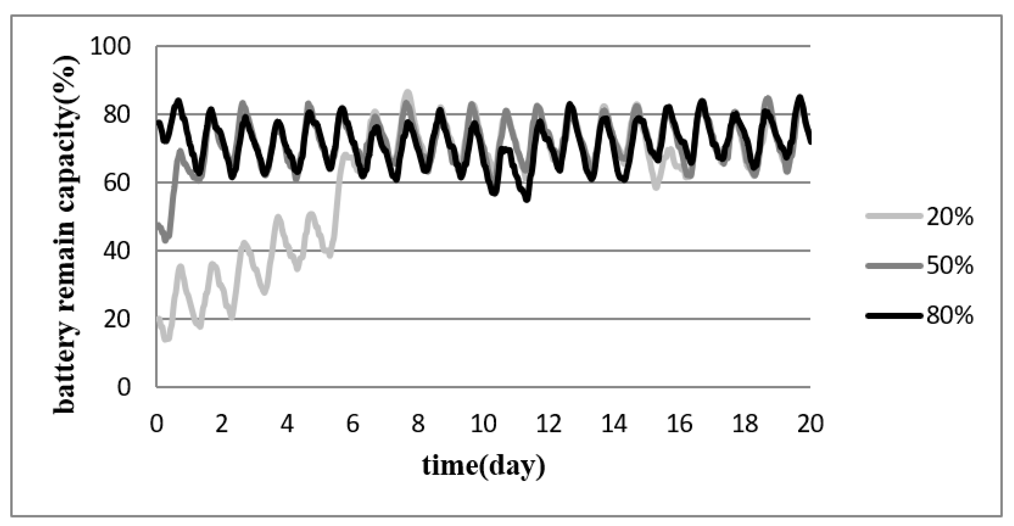
Figure 5 shows the experimental results of the proposed FQLDEM for sustainable operation of EHWSN with the initial battery energy of 20%, 50% and 80% for the first ten days. From the figure, it can be verified that the proposed method can maintain the battery remaining energy at 70% stably under different initial energy conditions. In Figure 5, it can be seen from the light grey line that when the energy is initially 20%, the proposed method can reach the expected battery energy of 70% on the sixth day. When the initial energy is 50% and 80%, the proposed FQLDEM can reach the expected energy on the second day.

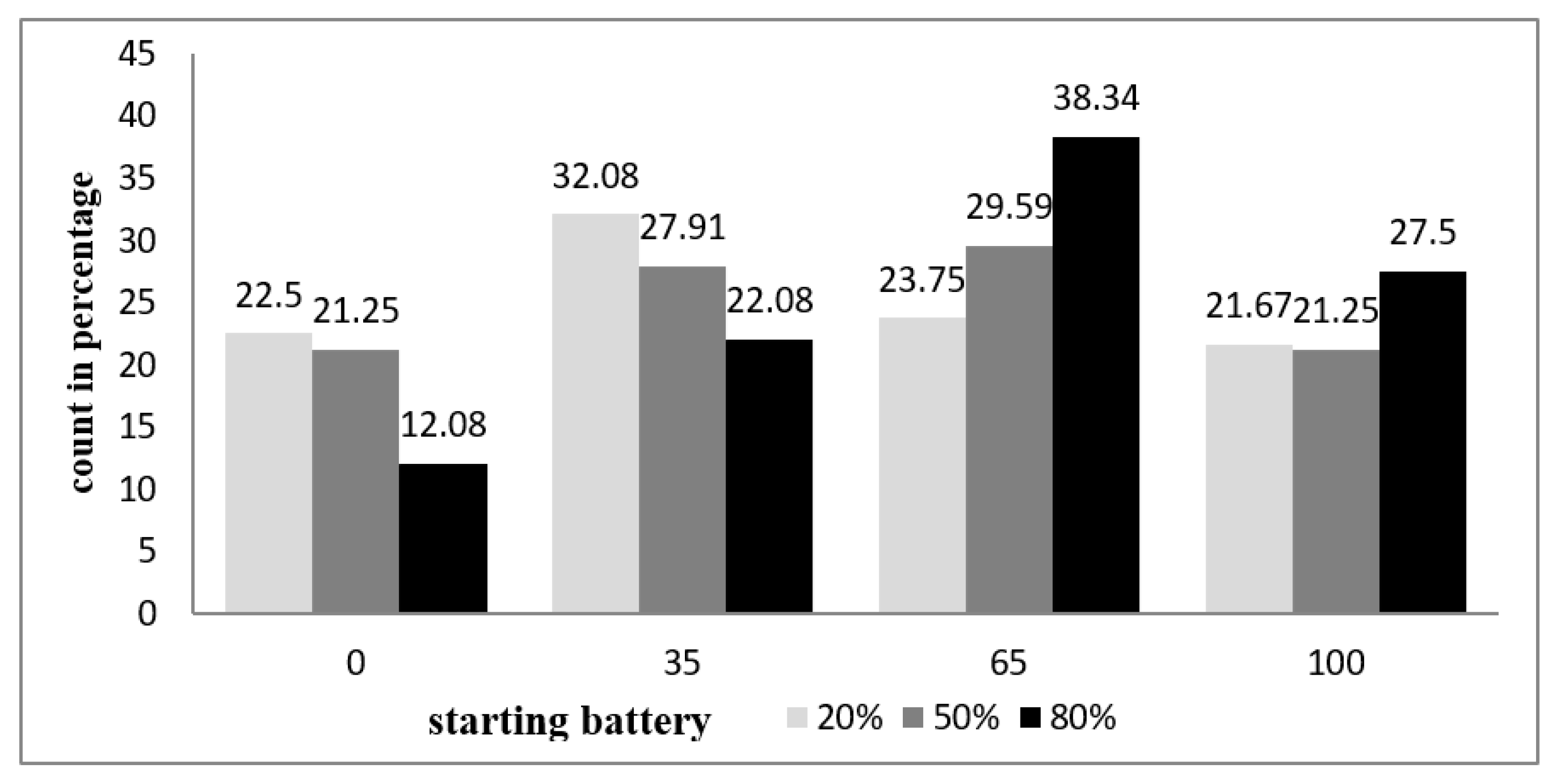
Figure 6 shows the number of selections of working duty cycle in percentage with different initial battery energy. According to Figure 6, the proposed FQLDEM method exhibits different working duty cycle selection strategies for different initial energy level. When the energy level is initially 20%, the selection of working duty cycles of 0% and 35% are higher. When the energy level is 50%, 35% and 65% are mostly adopted. When the initial battery energy is 80%, the selection of working duty cycles of 65% and 100% are higher. It can be seen from the above experimental results that the proposed method can adjust the working duty cycle according to different environmental conditions, and gradually learn and adjust the fuzzy rule base with the reward value, such that the energy-neutral operation of the EHWSN can be achieved and the target of the battery remaining energy is maintained.

4.2. Energy Neutrality Experiment of Comparing Methods

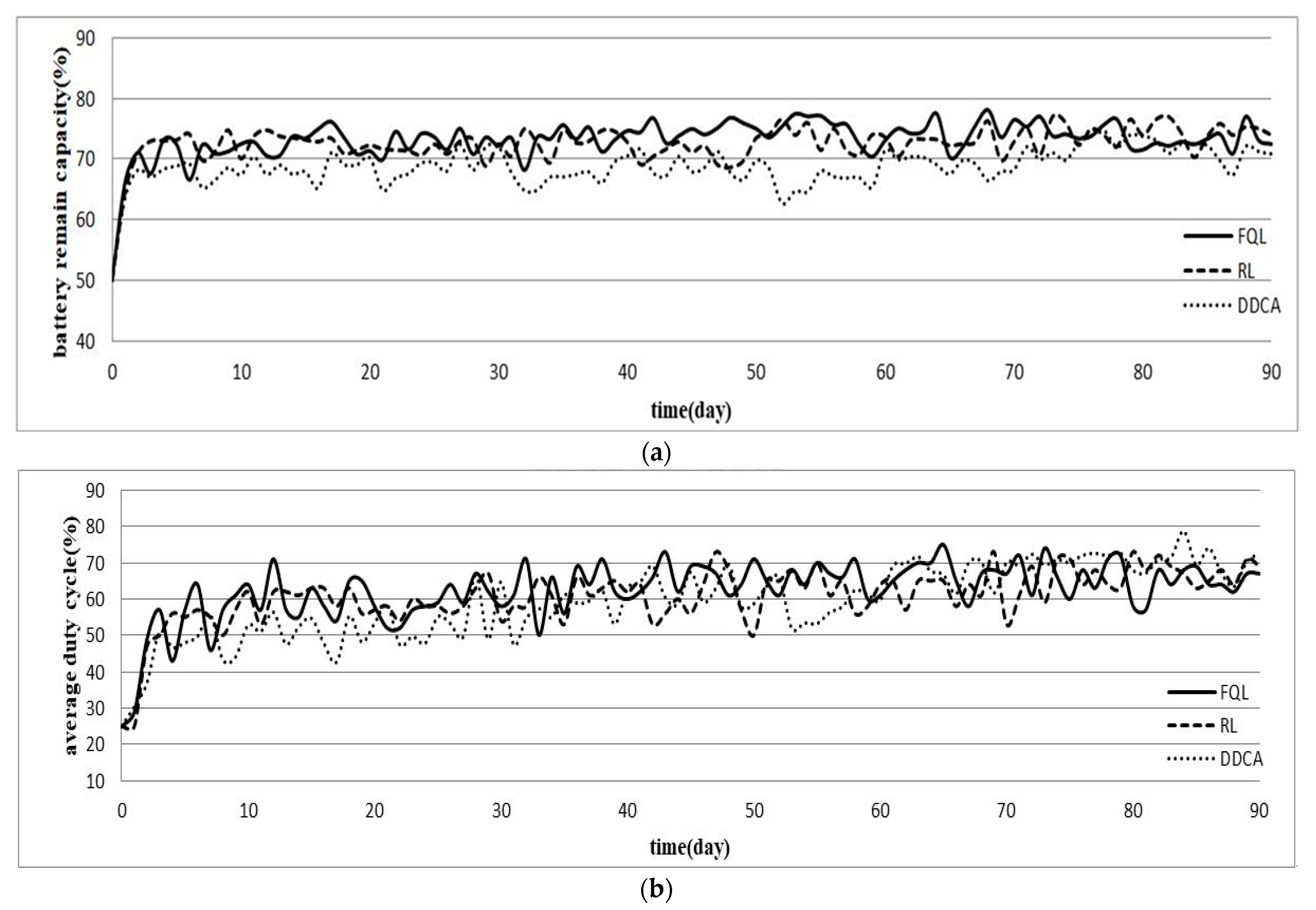
In this section, the experiment results of the proposed FQLDEM will be compared with those of the reinforcement learning (RL) energy management method [8] and the dynamic duty cycle adaption (DDCA) method [11]. The simulation time selection starts at the vernal equinox and ends on the summer solstice, experiment with the same simulated environment of 20%, 50%, and 80% of the initial battery energy, and the changes of the battery remaining energy and working duty cycle for a total of 90 days are recorded and compared. For illustration purposes, only the results of experiments with the same simulated environment of 50% of the initial battery energy are shown, as in Figure 7.

Comparison of Experimental Results and Discussions

It can be observed from Figure 7a that the FQLDEM can reach the expected energy on the second day, but because the FQLDEM is still learning in the early days, the battery energy changes slightly larger, which can be maintained between 70% and 76% until the 7th day. The RL method can also reach the expected energy on the second day and maintain the energy between 68% and 75% starting from the third day. The DDCA method approached the expected energy level on the third day, but the battery remaining energy cannot be stably maintained at 70%. It can be seen from the average working duty cycle chart in Figure 7b that when the initial energy is lower than the expected energy, both the FQLDEM and the RL method choose a lower working duty cycle strategy, such that the battery energy can be increased quickly. Hence, the working duty cycle of the FQLDEM and the RL method is no higher than 45% in the first two days during the energy increase period. After the battery energy is stable, the working duty cycle will be increased to consume excess energy. The DDCA method also uses a low working duty cycle in the early days, and the working duty cycle is increased due to the gradual excess of battery energy in the later period.

The experimental results of the second month are from the 31st to the 60th day as shown in Figure 7. Figure 7a shows that the remaining battery energy of the FQLDEM converges faster than the previous month and is maintained between 71% and 77%, whereas the RL method has a large energy reduction on the 32nd, 41st, and 48th days, and the DDCA method also has a large energy consumption on the 33rd and 52nd days. Figure 7b shows that the working duty cycle of the FQLDEM is slightly higher than the RL method for most of the time. The working duty cycle of the FQLDEM increases on the 32nd and 59th days and the battery energy is greatly decreased, but the working duty cycle is decreased on the next day such that the battery energy can be stabilized, whereas the working duty cycle obtained by the RL method changes a lot on the 32nd, 41st, and 48th days, which consequently affects the stability of the battery remaining energy. The working duty cycle of the DDCA method increases on the 32nd and 51st days, which exhibits the results of energy reduction.

The experimental results of the third month are from the 61st to 90th days. After a long period of training and learning, Figure 7a shows that the average remaining battery energy during this period no longer changes significantly. The FQLDEM’s battery remaining energy is maintained at 70~78%, whereas that of the RL method is maintained at 69~77%, and the DDCA method is maintained at 66~75%. From Figure 7b, it can be understood that in order to consume more electric energy, the average working duty cycle of both FQLDEM and RL methods is slightly higher than that of the previous two months, whereas the DDCA method has a higher working duty cycle, which reduces the remaining battery energy and is lower than those of FQLDEM and RL methods.

Based on the above experimental results,

Table 5. Results of energy neutrality experiment with 50% initial battery energy in three months for three comparative methods.

	Method	RL	DDCA	FQLDEM
Comparison Parameters
1st month	Average Remaining battery energy	72.01%	67.34%	71.96%
	Average Working Duty Cycle	56.6%	52.29%	57.27%
	Standard Deviation of Battery energy	2.01	2.41	2.30
	Battery energy Compared with FQLDEM	−0.6%	+6.86%
	Working Duty Cycle Compared with FQLDEM	+1.1%	+9.52%
2nd month	Average Remaining battery energy	72.49%	67.72%	74.3%
	Average Working Duty Cycle	61.63%	59.5%	64.9%
	Standard Deviation of Battery energy	2.13	2.15	2.04
	Battery energy Compared with FQL	+2.5%	+9.7%
	Working Duty Cycle Compared with FQLDEM	+5.3%	+9%
3rd month	Average Remaining battery energy	73.83%	70.85%	74.04%
	Average Working Duty Cycle	65.5%	69.74%	66.26%
	Standard Deviation of Battery energy	1.99	2.15	1.99
	Battery energy Compared with FQLDEM	+0.2%	+4.5%
	Working Duty Cycle Compared with FQLDEM	+1.1%	−4.9%

shows the comparison of energy neutral experiment with 50% initial energy for three months. It can be seen that although the proposed FQLDEM has a slightly lower average remaining energy in the first month than the RL method has, the FQLDEM has a steady increase in the following two months and is higher than the others. For the RL method of the period, it can be seen from the results of the average working duty cycle that the FQLDEM method slightly outperforms the RL method every month. In addition, compared with the DDCA method, the average remaining battery energy of the last month is slightly better than the average of the previous 2 months. The working duty cycle of FQLDEM is also higher than the DDCA method, but in the third month, DDCA increases the working duty cycle, which in turn increases the average working duty cycle value. Through the calculation of standard deviation for battery remaining energy, it can be seen that as time increases, the FQLDEM’s energy standard deviation continues to decrease, which means that the fluctuation degree of the battery energy is gradually reduced. Although the battery remaining energy of the RL method also tends to converge in the second month, the standard deviation of the battery remaining energy has increased slightly, and the standard deviation of the battery remaining energy of the DDCA method also gradually decreases over time, but it is slightly higher than that of the FQLDEM method.

4.3. Energy-Neutral Experiment with Required Total On-Demand Sensing Measurement

This experiment is to verify that not only the perpetual operation of the EHWSN can be effectively achieved by the proposed FQLDEM method, but the requirements of on-demand sensing measurement can also be met. Therefore, the experiment was conducted for two other comparing methods as well with the simulation time selection starts at the vernal equinox and ends on the summer solstice. The battery remaining energy and the change of the working duty cycle for a total of 90 days are recorded and the experimental results for three comparative methods are analyzed as well. In this experiment, the frequency of the demand for sensing measurement is moderate relatively, and the probability of low working duty cycle requirement is higher than that of the medium and high working duty cycles. The results of the experiment are shown in Figure 8.

Comparison of Experimental Results and Discussions

It can be seen in Figure 8a that the FQLDEM and RL methods maintain a stable energy level during this experimental period, whereas the DDCA method has a continuous decline in energy level on the 5th day. As shown in Figure 8b, it can be seen that the FQLDEM method can be slowly upgraded to meet 65% of the service quality control requirements in the early stage, and after the 12th day, it can be maintained to meet the 68% on-demand measurement requirements. The RL method maintains a steady rise and reaches about 73% on the 5th day. The DDCA method can reach 60% of the demand for on-demand measurement in the early stage, but it cannot maintain stability. It can be seen in Figure 8a that after a long period of training and learning, the battery energy of the FQLDEM method has stabilized at 70%. The RL method has a slight increase in energy on the 84th day and remains stable at 70% during other times. The battery remaining energy of the DDCA method also tends to be stable, but it is slightly lower than that of the other two methods. It can be observed in Figure 8b that both FQLDEM and RL methods can meet about 71% and 72% of on-demand sensing measurement requirements in the later stage of the experiment, whereas the DDCA method meets about 60% of on-demand sensing measurement requirements.

Based on the above experimental results for on-demand sensing measurement requirements, the result comparison of three methods can be summarized quantitively as

Table 6. Comparison of Low demand for on-demand sensing measurement experiment results for three comparative methods.

	Method	RL	DDCA	FQLDEM
Comparison Parameters
1st month	Average battery remaining energy	71.36%	64.48%	67.96%
	Average working duty cycle	56.63%	58.61%	58.53%
	Average on-demand measurement demand fulfillment rate	67.93%	55.27%	66.56%
	Energy offset to FQLDEM	−4.76%	+5.39
	Working duty cycle offset to FQLDEM	+3.35%	−0.13%
	Offset of on-demand sensing measurement demand fulfillment rate to FQLDEM	−2.01%	+20.4%
2nd month	Average battery remaining energy	72.94%	66.16%	68.75%
	Average working duty cycle	62.26%	63.23%	63.36%
	Average on-demand measurement demand fulfillment rate	72.86%	56.6%	68.7%
	Energy offset to FQLDEM	−5.74%	+3.9%
	Working duty cycle offset to FQLDEM	+1.76%	+0.2%
	Offset of on-demand sensing measurement demand fulfillment rate to FQLDEM	−5.7%	+21.3%
3rd month	Average battery remaining energy	72.56%	66.92%	70.03%
	Average working duty cycle	65.66%	66.38%	67.3%
	Average on-demand measurement demand fulfillment rate	72.93%	60.17%	70.9%
	Energy offset to FQLDEM	−3.48%	+4.6%
	Working duty cycle offset to FQLDEM	+2.49%	+1.38%
	Offset of on-demand sensing measurement demand fulfillment rate to FQLDEM	−2.78%	+17.8%

.

It can be seen from Table 6, when the demand for on-demand sensing measurement is low, the average remaining energy of the FQLDEM is slightly lower than that of the RL method by 3~4%, but its average working duty cycle is 2~3% higher than that of the RL method. The impact of imposing demand for on-demand sensing measurement for the FQLDEM is that the choice of fuzzy rules need to be trained by the Q-learning, hence FQLDEM tends to fulfill the on-demand working duty cycle and consequently sacrifices the battery remaining energy such that the values slightly fluctuate away from energy neutrality. As a result, the average on-demand sensing measurement demand achievement rate of the FQLDEM is moderate with that of the RL method. However, the average remaining energy of the FQLDEM is higher than that of the DDCA in 4~5% and the DDCA cannot maintain close to the expected energy level, yet the average working duty cycle of the FQLDEM is slightly higher than the DDCA method in the 2nd and 3rd month period.

5. Conclusions

In this study, a FQLDEM for perpetual operation of EHWSN is proposed. The research method is based on the fuzzy inference system, combined with the reinforcement learning theory to train its fuzzy rule library in adapting the sensing duty cycle for energy neutrality such that the perpetual operation of the EHWSN can be achieved. Experimental results of the FQLDEM shown that even when the demand for on-demand sensing measurement is imposed, not only a stable battery remaining energy can be maintained by the FQLDEM, but the demand for on-demand sensing measurement can also be met. It can be seen from comparing the experimental results with RL-based and DDCA methods that this proposed FQLDEM can maintain the EHWSN at a higher battery remaining energy level than the other two methods. In the on-demand sensing measurement demand experiment, although the average battery remaining energy of the proposed FQLDEM is sometimes moderate with the RL-based method, the working duty cycle of the FQLDEM increased slightly more than those of the RL-based and DDCA methods. The DDCA method is a dynamic programming method; therefore, its performance is easily affected when the environment and climate change, and therefore cannot maintain a stable battery energy. In conclusion, the proposed FQLDEM not only can stably maintain the perpetual operation of the EHWSN, but the system’s requirement for on-demand sensing measurement can also be met. The possible drawback of the FQLDEM is that it takes a certain amount of time to reach the convergent for the q value in the conclusion part of the FQL. To overcome this drawback and serve the purpose of off-line pre-training, one can train the FQLDEM with practical climate data for a certain time period and record the convergent q values for several times. By taking the average among the convergent q values from the pre-training period, a fast convergence reaching the expected battery state of charge can be achieved. Because this study only considers solar energy as the energy harvesting source, other renewable energy sources, such as wind energy, vibration energy, can also be included in the selection of energy harvesting sources in the future, and the FQLDEM can be applied to the hybrid EHWSN to achieve the perpetual operation of WSN as well.

References

- Sharma, H.; Haque, A.; Jaffery, Z.A. Maximization of wireless sensor network lifetime using solar energy harvesting for smart agriculture monitoring. Ad Hoc Netw. 2019, 94, 101966. [Google Scholar] [CrossRef]
- Kansal, A.; Hsu, J.; Srivastava, M.; Raghunathan, V. Harvesting aware power management for sensor networks. In Proceedings of the 43rd Annual Design Automation Conference, New York, NY, USA, 24–28 July 2006; pp. 651–656. [Google Scholar]
- Kansal, A.; Hsu, J.; Zahedi, S.; Srivastacva, M.B. Power management in energy harvesting sensor networks. ACM Trans. Embed. Comput. Syst. 2007, 6, 32. [Google Scholar] [CrossRef]
- Sutton, R.S.; Barto, A.G. Reinforcement Learning: An Introduction, 2nd ed.; The MIT Press: Cambridge, MA, USA, 2017. [Google Scholar]
- Oh, S.-Y.; Lee, J.-H.; Choi, D.-H. A new reinforcement learning vehicle control architecture for vision-based road following. IEEE Trans. Veh. Technol. 2000, 49, 997–1005. [Google Scholar]
- Valasek, J.; Doebbler, J.; Tandale, M.D.; Meade, A.J. Improved Adaptive–Reinforcement Learning Control for Morphing Unmanned Air Vehicles. IEEE Trans. Syst. Man Cybern. Part B 2008, 38, 1014–1020. [Google Scholar] [CrossRef] [PubMed]
- Hsu, R.C.; Liu, C.-T.; Wang, H.-L. A Reinforcement Learning-Based ToD Provisioning Dynamic Power Management for Sustainable Operation of Energy Harvesting Wireless Sensor Node. IEEE Trans. Emerg. Top. Comput. 2014, 2, 181–191. [Google Scholar] [CrossRef]
- Aoudia, F.A.; Gautier, M.; Berder, O. RLMan: An Energy Manager Based on Reinforcement Learning for Energy Harvesting Wireless Sensor Networks. IEEE Trans. Green Commun. Netw. 2018, 2, 408–417. [Google Scholar] [CrossRef] [Green Version]
- Zadeh, L.A. Fuzzy sets. In Fuzzy Sets, Fuzzy Logic, and Fuzzy Systems: Selected Papers by Lotfi A Zadeh; World Scientific: Singapore, 1996; pp. 394–432. [Google Scholar]
- Yager, R.R.; Zadeh, L.A. (Eds.) An Introduction to Fuzzy Logic Applications in Intelligent Systems; Springer Science & Business Media: Berlin/Heidelberg, Germany, 2012. [Google Scholar]
- Kerre, E.E.; Nachtegael, M. (Eds.) Fuzzy Techniques in Image Processing; Springer Science & Business Media: Berlin/Heidelberg, Germany, 2000. [Google Scholar]
- Ye, J. Fuzzy decision-making method based on the weighted correlation coefficient under intuitionistic fuzzy environment. Eur. J. Oper. Res. 2010, 205, 202–204. [Google Scholar] [CrossRef]
- Tektas, M. Weather forecasting using ANFIS and ARIMA models. Environ. Res. Eng. Manag. 2010, 51, 5–10. [Google Scholar]
- Harirchian, E.; Lahmer, T. Developing a hierarchical type-2 fuzzy logic model to improve rapid evaluation of earthquake hazard safety of existing buildings. Structures 2020, 28, 1384–1399. [Google Scholar] [CrossRef]
- Nebot, À.; Mugic Augica, F. Energy performance forecasting of residential buildings using fuzzy approaches. Appl. Sci. 2020, 10, 720. [Google Scholar] [CrossRef] [Green Version]
- Radwan, E.; Nour, M.; Awada, E.; Baniyounes, A. Fuzzy Logic Control for Low-Voltage Ride-Through Single-Phase Grid-Connected PV Inverter. Energies 2019, 12, 4796. [Google Scholar] [CrossRef] [Green Version]
- Shadoul, M.; Yousef, H.; Al Abri, R.; Al-Hinai, A. Adaptive Fuzzy Approximation Control of PV Grid-Connected Inverters. Energies 2021, 14, 942. [Google Scholar] [CrossRef]
- Berenji, H.; Khedkar, P. Learning and tuning fuzzy logic controllers through reinforcements. IEEE Trans. Neural Netw. 1992, 3, 724–740. [Google Scholar] [CrossRef] [PubMed] [Green Version]
- Juang, C.-F.; Lin, J.-Y.; Lin, C.-T. Genetic reinforcement learning through symbiotic evolution for fuzzy controller design. IEEE Trans. Syst. Man Cybern. Part B 2000, 30, 290–302. [Google Scholar] [CrossRef] [PubMed]
- Berenji, H.R.; Vengerov, D. A convergent actor-critic-based FRL algorithm with application to power management of wireless transmitters. IEEE Trans. Fuzzy Syst. 2003, 11, 478–485. [Google Scholar] [CrossRef]
- Wu, S.; Er, M.J.; Gao, Y. A fast approach for automatic generation of fuzzy rules by generalized dynamic fuzzy neural networks. IEEE Trans. Fuzzy Syst. 2001, 9, 578–594. [Google Scholar] [CrossRef]
- Glorennec, P.Y.; Jouffe, L. Fuzzy Q-learning. In Proceedings of the 6th International Fuzzy Systems Conference, Tianjin, China, 14–16 August 1997; pp. 659–662. [Google Scholar]
- Jouffe, L. Fuzzy inference system learning by reinforcement methods. IEEE Trans. Syst. Man Cybern. Part C Appl. Rev. 1998, 28, 338–355. [Google Scholar] [CrossRef]
- Kofinas, P.; Dounis, A.I.; Vouros, G.A. Fuzzy Q-Learning for multi-agent decentralized energy management in microgrids. Appl. Energy 2018, 219, 53–67. [Google Scholar] [CrossRef]
- Maia, R.; Mendes, J.; Araújo, R.; Silva, M.; Nunes, U. Regenerative braking system modeling by fuzzy Q-Learning. Eng. Appl. Artif. Intell. 2020, 93, 103712. [Google Scholar] [CrossRef]
- Zangeneh, M.; Aghajari, E.; Forouzanfar, M. A survey: Fuzzify parameters and membership function in electrical applications. Int. J. Dyn. Control 2020, 8, 1040–1051. [Google Scholar] [CrossRef]
- Preliminary Product Information Sheet Solar Module Power up 1. Available online: http://www.mrsolar.com/content/pdf/PowerUp/BSP-1-12.pdf (accessed on 4 March 2020).
- MICAz MPR2400CA Data Sheet. Available online: http://edge.rit.edu/edge/P08208/public/Controls_Files/MICaZ-DataSheet.pdf (accessed on 4 March 2022).
- OS08A10 Datasheet. Available online: https://www.ovt.com/products/os08a10-h92a-1b/ (accessed on 4 March 2022).
- GP700DHC NiMH Rechargeable Battery. Available online: https://cpc.farnell.com/gp-batteries/gp700dhc/battery-ni-mh-d-7ah-1-2v/dp/BT01867 (accessed on 4 March 2022).
Figure 1.
System architecture of the proposed FQLDEM for the EHWSN.
Figure 2.
The flowchart of the FQLDEM for EHWSN.
Figure 3.
Solar panel power supply for 10 consecutive days.
Figure 4.
Gaussian membership function of (a) solar panel energy harvesting signal and (b) battery remaining energy signal .
Figure 5.
Recordings of the battery remaining energy of the proposed FQLDEM for EHWSN with the initial battery energy of 20%, 50% and 80% for the first twenty days.
Figure 6.
Number of selections of working duty cycle in percentage.
Figure 7.
Comparison of energy neutral experiment with 50% initial battery energy (a) Average remaining battery energy, (b) Average working duty cycle value.
Figure 8.
Comparison of the medium demand of on-demand sensing measurement experiment. (a) Average remaining battery energy. (b) Average on-demand sensing measurement demand achievement rate.