
Analysis of Rostov-II Benchmark Using Conventional Two-Step Code Systems
by
 ,
,
Jaerim Jang
1, 
Mathieu Hursin
2,*,
Woonghee Lee
1,
Andreas Pautz
2,
Marianna Papadionysiou
2,
Hakim Ferroukhi
2 and
Deokjung Lee
1 1
Department of Nuclear Engineering, Ulsan National Institute of Science and Technology, 50 UNIST-gil, Eonyang-eup, Ulju-gun, Ulsan 44919, Korea
2
Nukleare Energie und Sicherheit, Paul Scherrer Institut (PSI), 5232 Villigen, Switzerland
*
Author to whom correspondence should be addressed.
Energies 2022, 15(9), 3318; https://0-doi-org.brum.beds.ac.uk/10.3390/en15093318
Submission received: 4 April 2022
/
Revised: 22 April 2022
/
Accepted: 25 April 2022
/
Published: 2 May 2022
(This article belongs to the Special Issue Computational Techniques of Nuclear Reactor Physics)
Abstract
:This paper presents the steady state analysis of the Rostov-II benchmark using the conventional two-step approach. It involves the STREAM/RAST-K and CASMO-5/PARCS code systems. This paper documents a comprehensive code-to-code comparison between Serpent 2, CASMO-5, and STREAM at the lattice level for the different fuel assemblies (FAs) loaded in the Rostov-II core; and between Serpent 2, PARCS, and RAST-K at the core level in 2D. Finally, the 3D results of both deterministic models are compared to the steady state measurements of the Rostov-II benchmark. With respect to the measurements available in the Rostov-II benchmark, comparable accuracy (30 ppm difference in boron concentration, 2% assembly power) with an industrial calculation scheme (BIPR8) are reported up to 36.73 EFPDs. The calculations reported in the paper showed that the modeling of the resonance self-shielding in the lattice code as well as the geometrical modeling of the reflector are key for an accurate solution (reducing the in-out power tilt). At the core simulator level, a fairly crude 1D reflector model appears to be enough. Overall, this paper provides the detailed models and conditions used in STREAM/RAST-K and CASMO-5/PARCS, and accurate calculation solution for the Rostov-II benchmark with STREAM/RAST-K and CASMO-5/PARCS compared with measurement.
1. Introduction
Currently, a total of 71 Vodo-Vodyanoi Energetichesky Reactors (VVERs) are operated in 24 countries [1,2]; planning is underway for 32 more plants [3]. As the market size of the VVER reactor grows, hexagonal solvers for VVER analysis have been developed in various commercial and academic code systems: HEXTRAN [4], PARCS [5,6], SIMULATE-5 [7], DYN3D [8], KIKO3D [9], BIRP-8 [10], and SKETCH-N [11]. Verification and validation studies have been performed based on various benchmarks: PHARE SRR 1/95 project [12], VALCO project [13], V1000CT benchmark project [14], OECD/NEA benchmark problems (Kalinin-3 [9], and Rostov-II [10]) and AER benchmark books [13]. The Rostov-II benchmark has been recently developed by OECD/NEA to allow validation of novel high-fidelity multi-physics codes developed by various international projects [10], including the consortium for advanced simulation of LWRs (CASL), nuclear energy advanced modeling and simulation (NEAMS), and NURESAFE. Currently a BIPR8 [15] solution to the benchmark is provided by the Kurchatov Institute. BIPR8 has been widely used for VVER analysis [16,17,18].
This paper presents the analysis of the Rostov-II benchmark [10] using conventional two-step approach code systems: CASMO-5/PARCS [19,20], and UNIST in-house code system STREAM/RAST-K [21,22]. This paper has two main purposes. One is the verification and validation (V & V) of the calculation scheme of STREAM/RAST-K and CASMO-5/PARCS for VVERs. The other one is to provide two conventional solutions to the Rostov-II benchmark.
This paper documents a comprehensive code-to-code comparison between Serpent 2, CASMO-5, and STREAM at the lattice level, for the different fuel assemblies (FAs) loaded in the Rostov-II core; and between Serpent 2, PARCS, and RAST-K at the core level in 2D. Finally, the 3D results of both deterministic models are compared to the steady state measurements of the Rostov-II benchmark.
STREAM/RAST-K is the UNIST in-house two-step code system. A VVER analysis module has been developed based on the triangular polynomial expansion nodal (TPEN) kernel [23], to extend the application area to reactors with hexagonal geometry. The core solver RAST-K has been verified using the Kalinin-3 and VVER-440 [24,25] benchmarks. As shown in previous studies, RAST-K has comparable accuracy with other code systems like PARCS, ATHLET/KIKO3D, and DIF [24,25]. Additionally, a conventional VVER analysis scheme is under development at Paul Scherrer Institute (PSI) using CASMO-5 and PARCS [26]. Both CASMO-5 and PARCS have been actively used worldwide for analysis of nuclear power plants. CASMO-5 has been developed by Studsvik Scandpower Incorporated [19] and has been used for analysis of a VVER-1000 with SIMULATE [7]. The VVER analysis module ported in PARCS has been verified with few-group constants generated by HELIOS, nTRACER, and Serpent 2 [6,26].
The remainder of this paper is arranged as follows. Section 2 describes the code systems, and Section 3 presents the description of the Rostov-II benchmark. Section 4 contains the verification results at the assembly and 2D core level. Section 5 deals with the 3D full core results, the comparison to an existing solution produced by BIPR8, and actual measurements performed at the plant: radial and axial power distribution, as well as boron concentration in the coolant, are used as quantities of interest.
2. Code Systems
2.1. STREAM/RAST-K
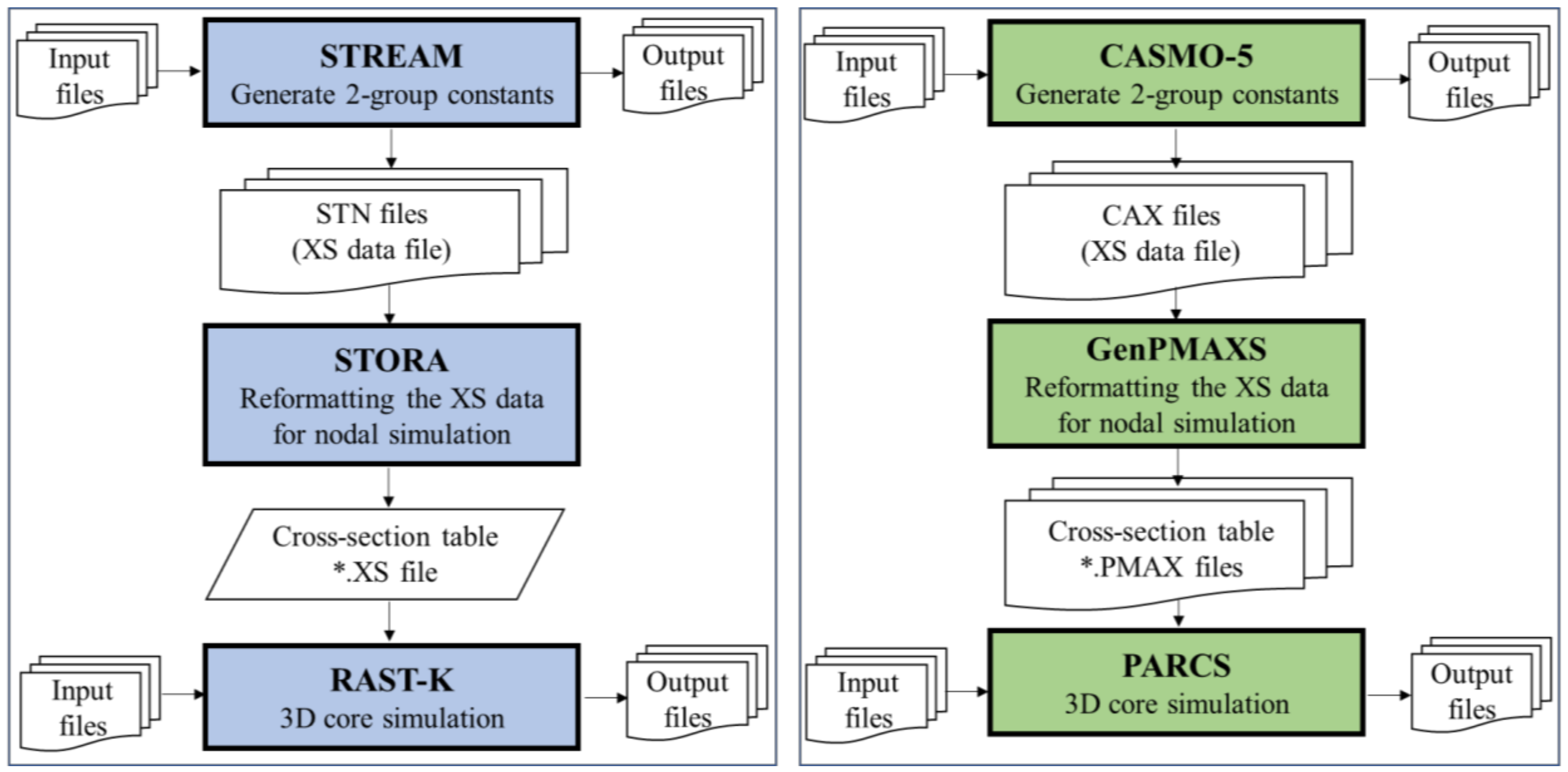
The STREAM/RAST-K two-step approach code system has been utilized to model various types of nuclear reactors (APR-1400 [27], OPR-1000 [27], two-loop and three-loop Westinghouse nuclear power plants [28], and small modular reactors [29,30]). To extend its application area, a VVER analysis module has been recently developed in STREAM/RAST-K. Figure 1 displays the flowchart of STREAM/RAST-K. Few group constants are generated by STREAM and are formatted using the linking code STORA (STREAM TO RAST-K) [27]. The 3D core simulation is performed by a two-group nodal diffusion code, RAST-K. Symbol of * in the figure means the all files (i.e., *.XS means the files with contains the ‘.XS’ letters in end of file name).
STREAM uses the method of characteristic (MOC) for solving the neutron transport problem. The pin-based slowing down method (PSM) is used for the resonance treatment [31,32]. The library uses a 72 energy group (10−5 eV to 20 MeV) structure, with 39 resonance energy groups (0.3 eV to 24,780 eV) [33]. In the present paper, the library is based on the ENDF/B-VII.0 library [34]. Finally, the kappa values (energy released per fission for each fissionable isotope) come from Origen-2 [35]. STREAM uses the coarse mesh finite difference (CMFD), and provides the parallel calculation mode for acceleration as option. Depletion calculations are performed based on the Chebyshev Rational Approximation Method (CRAM). A predictor-corrector algorithm is used for depletion, similar to Serpent 2. The depletion chains of 1640 isotopes are considered. The quadratic depletion method is used for gadolinium isotopes. In addition, the number density and microscopic cross sections of 36 isotopes are provided for microscopic depletion calculations ported in RAST-K [27]. The details of the case matrix for VVER analysis (branch and depletion conditions) are presented in reference [27]. The hexagonal geometry solver of STREAM has been verified with cross sections generated by the TULIP code for the C5G7 [36] and OECD-NEA SFR numerical benchmark [37].
The hexagonal geometry analysis solver in RAST-K is based on multi-group CMFD acceleration with triangular-based polynomial expansion nodal method (TPEN) [22,23]. The TPEN kernel ported in RAST-K has been successfully verified with VVER-440 [24] and VVER-1000 (Kalinin unit 3) benchmark problems [25]. RAST-K performs microscopic depletion calculations considering 36 isotopes (i.e., 22 of heavy nuclides and 12 of fission products). The micro-depletion solver is developed based on CRAM [27]. The micro-depletion solver has been verified with 58 spent fuel pins, and the number densities of the most important isotopes are within ±4%, as shown in reference [38]. The simplified one-dimensional single channel thermal-hydraulic feedback (TH1D) solver is used to provide T/H feedback in this paper. Assembly discontinuity factors (ADF) and corner flux discontinuity factors (CDF) are used in all reported calculations.
2.2. CASMO-5 and PARCS
Figure 1 presents the flowchart of the CASMO-5/PARCS code system. CASMO-5 generates the few-group constants for 3D core simulation, and GenPMAX [39] is used as linking code, to format the few-group constants produced by CASMO-5. The 59 branches (trees) and one reference calculation are used for generation of FA few-group constants: 59 branch conditions are composed by 4 branches of control rod (CR), 32 branches of moderator density, 14 branches of boron concentration, and 9 branches of fuel temperature. PARCS version 3.3.1 is used in this paper. CASMO-5 uses the 586 energy-group ENDF/B-VII.0 library (i.e., e7r0.125.586 library) [34], with 41 resonance groups (the range of energy groups is 10.0 eV to 9118 eV). During the 3D core simulation, internal T/H feedback scheme is used in both of PARCS [40] and RAST-K calculation.
2.3. Serpent 2
The code Serpent 2.1.27 [41] is used to provide reference results for code-to-code comparison at the assembly level and for 2D full core geometries. Serpent 2 is a 3D continuous-energy neutron physics code for particle transport based on the Monte Carlo method. This code has been developed at VTT since 2004, and has been utilized by 809 registered users in 201 organizations for neutronic analysis of reactors [42]. Serpent 2 has been used for 3D full core analysis of VVERs [43]. In addition, few-group constants generated by Serpent 2, have been used for 3D core simulations in previous studies [44,45]. A continuous-energy neutron cross-section library based on the ENDF/B-VII.0 [34] nuclear data is used for the calculations in this paper.
3. Description of Rostov-II Benchmark Problem
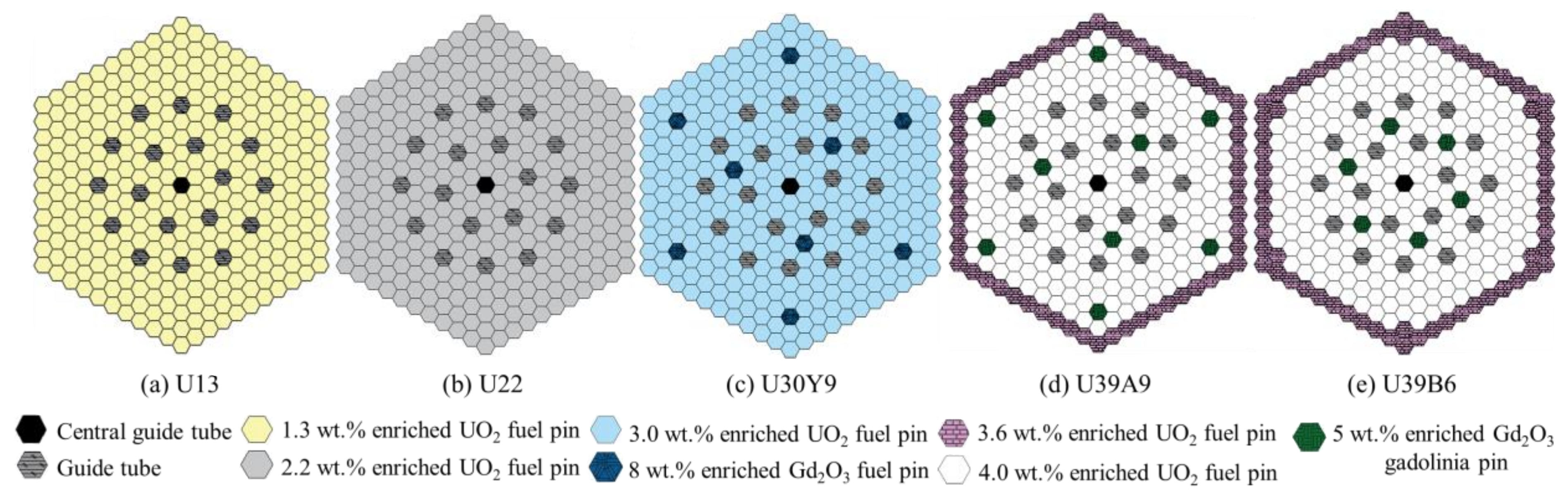
The Rostov-II reactor is a VVER-1000 type reactor, which has been operated since 2010 [46]. The detailed specifications were obtained from the benchmark description [10]. This section deals with specification of FA, core, reflector, and control rod models for analysis of Rostov-II benchmark. Figure 2 presents the radial layouts of five different FAs loaded in the Rostov-II reactor. Table 1 contains the general specifications of the Rostov-II reactor, and Table 2 presents the detailed information of Rostov-II fuel assemblies. A total of 163 fuel assemblies are loaded in the Rostov-II reactor; each assembly consists of 312 fuel rods.
Detailed FA models are presented in Section 3.1. Section 3.2 contains the reflector models, and Section 3.3 deals with the control rod model used in 3D simulation.
3.1. Effect of the Geometry Approximations at the Lattice Level
The current hexagonal analysis solver ported in STREAM has a limitation in modeling the central helium gap and guide tubes (i.e., a radius of guide tube is larger than the fuel pin pitch). For this reason, two approximations were used when modeling the FA. Figure 3 presents the approximated models of the UO2 fuel pin and guide tube. Figure 3a–c are nominal models of the UO2 fuel pin and the guide tube. Figure 3b,d are the approximated models. In the approximated model, the central helium hole (R1) and the fuel material (R2) are homogenized (R6) by using the volume ratio: the number density is defined using the relationship of VR1 * NDR1 + VR2 * NDR2 = VR6 * NDR6, where V is the volume and ND is number density. A total of 18 guide tubes and the central instrument tube have larger outer radius compared with the fuel pitch, namely R7 region of Figure 3c. The volume ratio was used to generate the approximated model, and the outer radius of the guide tube is changed to 0.6370 cm (R8 of approximated model) from 0.6500 cm (R7 of nominal model). The total mass is the same in the nominal model and the approximated model.
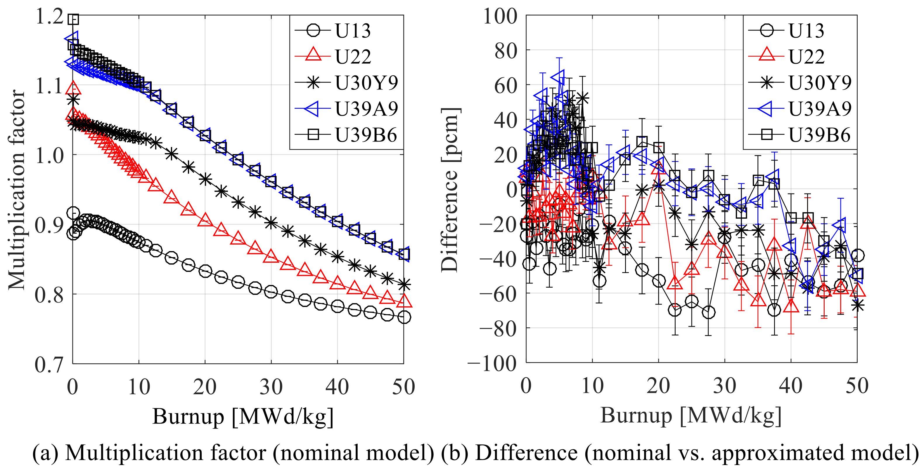
To assess the effect of the approximated models in fuel assembly calculations, a sensitivity study was performed using Serpent 2. Table 3 contains the calculation conditions, and Figure 4 illustrates the results. The k-inf discrepancies are within ±71 pcm for the entire exposure range considered. Figure 3b contains the differences between the nominal model and approximated model (the reference is the nominal model). The geometrical approximations involved in STREAM are shown to have only a minor effect on the reactivity of the FA. The approximated model is used for all calculations in this paper. To maintain the consistency, FA models of CASMO-5 are also designed with the approximated models. In addition, the effect of approximated models in terms of radial power for the 2D core model is within ±0.64%. Details are provided in Appendix A. Comparison is performed with Serpent 2, and the difference of multiplication factor is 2 pcm. Approximated models have a negligible effect on the multiplication factor and radial power in core calculation.
3.2. Reflector Models for Two-Step Approach
This section presents the reflector models for two-step approach calculation. Three different radial reflector types (1D, 2D, and core type) are involved. The 1D, 2D, and core type radial reflectors are shown in Figure 5, Figure 6 and Figure 7, respectively. The 2D type and core type reflector models are provided the XS data based on single assembly calculation and full core model, separately. The sensitivity study about the radial reflector modeling is presented in Section 4.2.2. Smeared reflector material is used for the design of 1D radial reflector, as shown in Figure 5c. The reflector model is produced in Cartesian geometry, as shown in previous study [47]. Figure 6 presents the five different 2D radial reflector models, which are composed of pin-wise smeared materials. The 2D reflector model is designed according to reference [48]. The central red hexagonal mark represents the reflector positions for which the homogenized few group constants are produced. The nominal core type reflector (Figure 7b) is generated by 2D transport calculations with CASMO-5 and STREAM. The reflector is designed based on pin-wise homogenized material, as shown in Figure 7c: the water holes in the heavy reflector (upper graph) are approximated as pin-wise homogenized regions (lower graph).
The active height of the fuel is 370 cm. It is divided in 20 axial layers of 18.5 cm thickness in the diffusion solvers. Two 37 cm thick reflectors are used for both the top and bottom regions of the core. Due to the lack of detailed information about the axial reflectors in the Rostov-II specifications of version 1.5, the description of the axial reflectors of the X2 reactor are used [43]. Axial reflectors are modeled similarly to the 1D radial reflectors. Figure 8 presents the smeared axial reflector model. Figure 8c contains the thickness of each reflector material, and Figure 8d presents the volume ratio of each reflector material. Assessment of designed axial reflectors is performed in Section 5 with the 3D Rostov-II model.
3.3. Control Rod Model
Figure 9 presents the radial layout of the Rostov-II reactor [10]. Figure 9a shows the loading pattern of the Rostov-II reactor, and Figure 9b contains the radial control rod bank positions of Rostov-II. The control rod bank #10 is moved to adjust the excess reactivity during the 3D core simulation. Figure 10 presents the axial configuration of two different CR models: nominal and simplified CR models. The nominal CR model consists of B4C and Dy2O3-TiO2, and the geometry is shown in Figure 10a. The simplified CR model is only built with B4C and the configuration is shown in Figure 10b. The material in the tip region is the difference between the nominal and simplified CR model: Dy2O3-TiO2 of the nominal tip model is replaced by B4C in the simplified CR model.
4. Verification Results
This section contains the verification results for FA and 2D full core calculations. FA results are presented in Section 4.1, and 2D core results in Section 4.2. The analysis at the FA level is focused on the assessment of the STREAM and CASMO-5 respective performances against a reference solution produced with Serpent 2. The quantities of interest are k-inf and the few-group constants. Then 2D full core calculations are carried out and their results are compared to Serpent 2 in terms of k-inf and radial power distributions.
Unless otherwise mentioned in the text, STREAM and CASMO-5 used the inscatter-corrected transport cross section, the thermal expansion was not considered, and the 238U resonance up-scattering correction was turned off for consistency with Serpent 2. General calculation conditions are presented in Table 3. Serpent 2 used a total of 48,000,000 neutron histories, i.e., 400,000 neutrons per cycle with 120 cycles (20 inactive and 100 active). The standard deviations are around 10 pcm and 0.3% in terms of multiplication factor and pin power solutions, respectively.
4.1. Fuel Assembly Calculation
Section 4.1.1 presents the single transport calculations for various conditions. Section 4.1.2 contains the depletion results, and Section 4.1.3 presents the comparison of few-group constants.
4.1.1. Steady State Calculations under Various Conditions
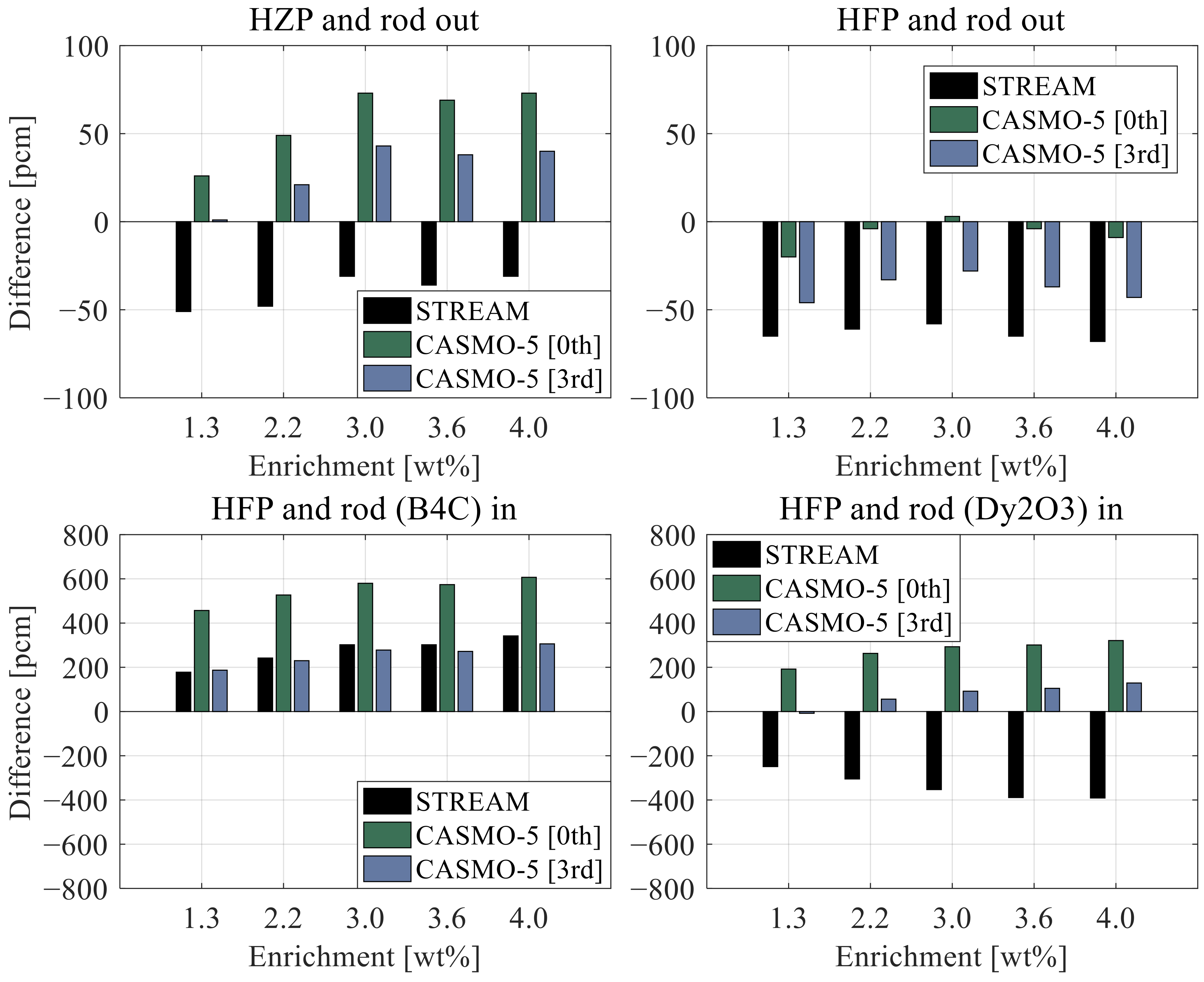
This section presents a comparison of STREAM, CASMO-5, and Serpent 2 k-inf for all FA types at various conditions. Specifically, the following tests are carried out: (1) rod out calculation at hot full power (HFP), (2) B4C rod in at HFP, (3) Dy2O3-TiO2 rod in at HFP, and (4) hot zero power (HZP). Figure 11 presents the comparison of multiplication factors and layouts of FAs used for calculation. Fuel temperature was set as 900 K in case (1), (2), and (3); 600 K was used in case (4). Moderator temperature and boron concentration are 600 K and 1000 ppm, respectively. Five different fuel enrichments are used for comparison: 1.3 wt.%, 2.2 wt.%, 3.0 wt.%, 3.6 wt.%, and 4.0 wt.%. During this sensitivity study, burnable absorber (e.g., gadolinia) was not involved in the calculation, and approximated control rod models were used. Table 3 contains the calculation conditions of STREAM and CASMO-5. Two CASMO-5 solutions are provided with different Pn-scattering orders: 0th (isotropic scattering with transport correction) and 3rd. The results of the 3rd order case give a more accurate solution with respect to Serpent 2; specifically, the control-rod-in caseshave high sensitivity in the Pn-scattering order [49]. The different trends observed between CASMO-5 and the STREAM are caused by the different resonance self-shielding methods involved. STREAM uses the pin-based pointwise energy slowing-down method (PSM), while CASMO-5 uses a distributed resonance integral (DRI) approach [19,31]. The observed k-inf underestimation in STREAM with respect to CASMO-5 is consistent with previous studies [31]. Detailed information about the Figure 11a to 11d are presented in Appendix A.
Finally, it is clear in Figure 11 that STREAM has difficulty predicting capture in the Dy2O3-TiO2 rods accurately. These differences are most likely due to the energy discretization used in CASMO-5 and STREAM. The notation of 0th and 3rd in the CASMO-5 labels of Figure 11 correspond to the 0th and 3rd order Pn-scattering, respectively. For the rod-in case, 18 guide tubes are filled with control rods. The reference is the Serpent 2 solution, and absolute differences are presented in the figure.
Figure 12 presents the energy boundaries of 72 groups and 586 groups used in STREAM and CASMO-5 [50]. The capture cross sections of 162Dy and 10B are included in this figure. CASMO-5 covers the first resonance of 162Dy with narrow energy intervals, and no additional self-shielding treatment is required. In STREAM, self-shielding treatment is needed, and it introduces fairly large discrepancies with respect to the Monte Carlo solution. Such discrepancies should have a negligible effect on 3D core simulations since Dy2O3-TiO2 is only encountered in the tip of the control rods. Details are presented in Section 5.
4.1.2. Depletion Calculations
This section contains verification results of STREAM and CASMO-5 in FA depletion using Serpent 2 as a reference. Calculation conditions are described in Table 3. Figure 13 presents the evolution of the k-inf discrepancies with respect to a Serpent 2 solution for STREAM and CASMO-5 as exposure increases. In Figure 13a, Serpent 2 Q values [51] are used in STREAM. In Figure 13b, Origen-2 Q values are used in STREAM. Figure 13c illustrates the differences between CASMO-5 and Serpent 2. CASMO-5 uses the exposure dependent Q values as described in reference [52]. The differences between STREAM and Serpent 2 are within ±200 pcm with Origen-2 Q values (default option) and are within ±300 pcm with consistent Q values from Serpent 2. In addition, the difference between CASMO-5 and Serpent 2 are within ±300 pcm. This result is similar to previous studies [53,54]. As shown in a previous VERA 1C benchmark analysis [53,54], the use of Origen-2 Q-value leads to higher multiplication factor results than when using the Serpent 2 Q-value cases. As STREAM tends to produce lower multiplication factors than Serpent 2, the use of Origen-2 Q helps reduce the discrepancies between both codes.
Figure 14 contains the difference of pin-wise radial power between STREAM and Serpent 2; U13 FA and U22 FA are used for comparison. The radial power discrepancies are within ±1.3%. Monte Carlo uncertainties in terms of radial power are around 0.3%. Figure 14b,c present the radial power distribution at 10 MWd/kg, and Figure 14f,g show the radial power distribution at 50 MWd/kg. Figure 14d,h contain the relative difference of pin power. Figure 14a,e present the maximum, minimum, and root mean square differences of pin power in U13 and U22 FAs as burnup proceeds. The same analysis has been carried out with CASMO-5 (not shown here for the sake of conciseness) and produces similar results: With respect to Serpent 2, CASMO-5 pin power distributions have 0.51% and 0.42% root mean square (RMS) difference at 10 MWd/kg and 50 MWd/kg, respectively. These results are in line with the typical agreement between deterministic and Monte Carlo codes for PWR assembly problems [55].
4.1.3. Few-Group Constants Comparison
Figure 15 contains the comparison of the few-group constants of STREAM and CASMO-5 compared with Serpent 2. U22 and U39A9 FAs are involved in the comparison. The considered burnup range is 0 to 50 MWd/kg. Group 1 and 2 are the fast and thermal energy groups, respectively. Four different parameters were compared in this study: (1) diffusion coefficient, (2) absorption cross section, (3) removable cross section, and (4) nu-fission cross sections. is the removable cross section calculated by Equation (1) [44].
where the and are the flux of group 1 and group 2, respectively. and are the scattering cross sections. CASMO-5 and STREAM use the inflow transport correction and CM method [49,56] to determine the diffusion coefficients. Serpent 2 uses the hydrogen transport correction curve reported in previous studies [57,58] for the determination of the diffusion coefficients. As shown in the Figure 15, STREAM and CASMO-5 show comparable accuracy with respect to Serpent 2 for few-group constants, with relative differences in the range of ±1% over the exposure range considered. In CASMO-5, the largest difference is observed for the thermal group diffusion coefficient; this is consistent with previously published results [57] targeting PWR lattices. Since the transport cross section affects the power distribution, as mentioned in previous studies [45,57], a detailed comparison is presented in Section 4.2 to assess the magnitude of these discrepancies on the power distribution in VVER type geometries.
4.2. Two-Dimensional Core Results
This section contains the verification results for 2D core calculations. Two main comparisons are contained in this section. One is the comparison of the 2D full core transport results (generated by the lattice codes directly) against Serpent 2, and the other is the comparison of the two-step code systems with Serpent 2.
4.2.1. Transport Solutions
The 0th order Pn scattering with a transport corrected total cross section was used for the CASMO-5 and STREAM calculations. For the Serpent 2 solution, a total of 1,256,000,000 neutron histories were used (i.e., 400,000 neutrons per cycle, 3000 active cycles, and 140 inactive cycles). It resulted in a standard deviation for a multiplication factor of 2 pcm. In addition, average standard deviations for FA and pin power are 0.074% and 0.8%, respectively.
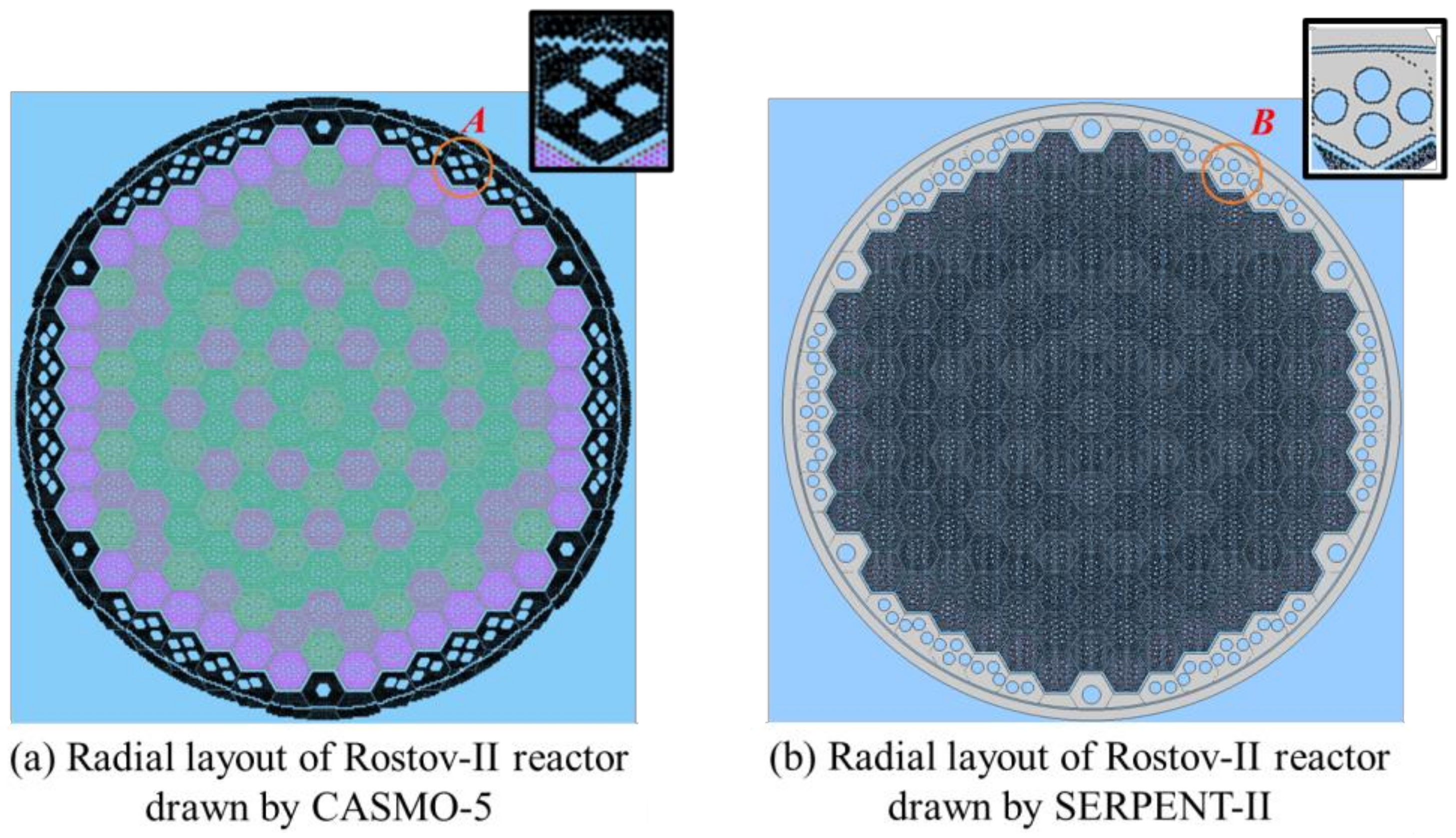
Because STREAM and CASMO-5 cannot model a water hole model of circular geometry in baffle region (see Figure 16b), a simplified reflector model was built using homogeneous pins, preserving the total mass of the reflector materials. The density and volume of the materials are changed according to equation of Nwater × Vwater + Nbaffle × Vbaffle = Nsmeared × Vsmeared, where the N is the number density and V is the volume. The simplified model is shown in Figure 16a, and is used in 2D calculations of STREAM, CASMO-5, and Serpent 2. Table 4 contains the calculated multiplication factors associated with the different calculation cases performed for a range of fuel temperature, moderator temperature, and boron concentration conditions. STREAM and CASMO-5 have within ±37 pcm and ±89 pcm difference compared to Serpent 2, respectively. Radial power profile is compared in Figure 17. Figure 17a contains the radial power distribution of Serpent 2. Figure 17b,c present the relative differences with respect to Serpent 2, of CASMO-5 and STREAM, respectively. The RMS difference of CASMO-5 from the Serpent 2 reference solution is 1.62% and 1.07%, at the assembly and pin level, respectively. For STREAM, the RMS difference is reduced to 0.7% both at the assembly and pin level (see Table 5 for details). These results are in-line with previously published studies, such as the comparison of nTRACER with the Monte Carlo code, McCARD [59] (1.20% RMS), or with Serpent 2 (1.8 % RMS) [26]. The CASMO-5 results are worse than the STREAM ones due to the different resonance treatment. To assess the effect of resonance treatment in radial pin power distribution, a comparison with different resonance treatment is performed with STREAM. PSM and Stamm’ler equivalent two-term method (EQ 2-term) [60] are considered, as the latter is similar to what is used in CASMO-5. As shown in Figure 18, the discrepancies in terms of pinpower due to the different resonance treatment methods are within ±1.6%, e.g., the same range than the discrepancies observed between STREAM and CASMO-5, which can then be explained by the resonance treatment differences.
The effect of the reflector modeling on the pinpower distribution is assessed through two Serpent 2 calculations performed with the simplified and nominal models (see Figure 16a,b). The results are shown in Figure 19: RMS difference is 1.44%, and the maximum differences are found next the edge of reactor (nearby baffle). This result represents that homogenized material description of the heavy reflector could produce significant radial power differences in regions close to the reflector.
4.2.2. Two-Step Calculations
This section presents the verification results of conventional two-step code systems, CASMO-5/PARCS and STREAM/RAST-K. As shown in the previous section, the model of the radial reflector strongly affects the power distribution. Various approaches are considered to produce the reflector cross sections in the two-step calculations: the 1D, 2D, and core type radial reflector models introduced in Section 3.2 are tested in this section.
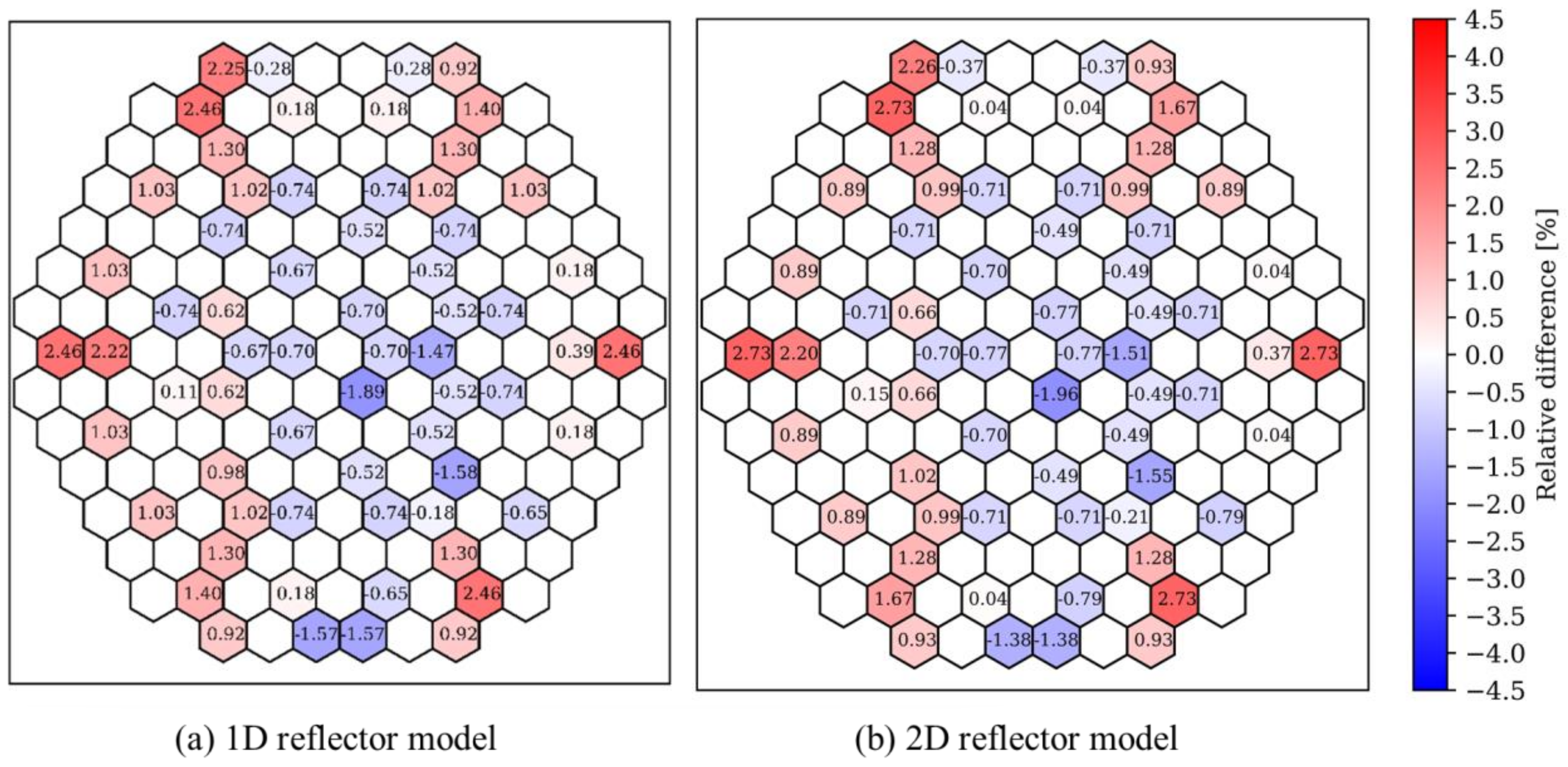
Fixed calculation conditions are used in the 2D core simulations: moderator temperature of 600 K, fuel temperature of 900 K, and boron concentration of 1000 ppm. Figure 20 presents the radial power differences of PARCS compared with CASMO-5 for the three different reflector modeling approaches. The 2D radial reflector model has the lowest in-out tilt, as shown in Figure 20. Although the 1D reflector model has less in-out tilt compared with core reflector model, the accuracies of 1D and core type reflector are similar.
Table 6 contains the summary of radial power differences compared with Serpent 2 assuming a simplified radial reflector model. Calculations with 1D, 2D, and core radial reflector models have results of similar accuracy. Both of CASMO-5/PARCS and STREAM/RAST-K calculations have good performance with 1D radial reflector models. As a result, 1D radial reflector models are used for the 3D core simulations in this paper.
5. Validation Results
This section describes the comparison of the STREAM/RAST-K and CASMO-5/PARCS 3D full core models with measurements during a part of the first Rostov-II cycle. The calculation conditions are presented in Table 3. Fundamental mode buckling calculation was performed for the generation of few-group constants. The 238U resonance up-scattering correction was turned on. As suggested in the benchmark specifications, the calculations are performed without the thermal expansion of fuel and cladding [10].
The locations of the CR banks are presented in Figure 9; only bank #10 is moved during the considered part of the reactor cycle. As described in Section 3.3, a simplified CR model is used. Fuel and coolant thermal hydraulic parameters (temperatures, water density) are obtained using TH1D model in RAST-K, while a similar approach is used in PARCS.
Boundary conditions are obtained from the reference [10,16]: control rod positions are from the reference [16]; the evolution of the thermal power from the reference [10]. A constant flowrate of 18,551.37 kg/s and inlet temperature of 292.2 °C are used as recommended from the Rostov-II benchmark [10] specifications. The first part of the Rostov-II first reactor cycle is simulated from 0 to 36.73 EFPDs. Four quantities of interest are compared in this section: (1) critical boron concentration, (2) outlet moderator temperature, (3) Doppler fuel temperature, and (4) radial and axial power profile. The 1 g/kg boron concentration is converted as 174.88 ppm according to the reference [43].
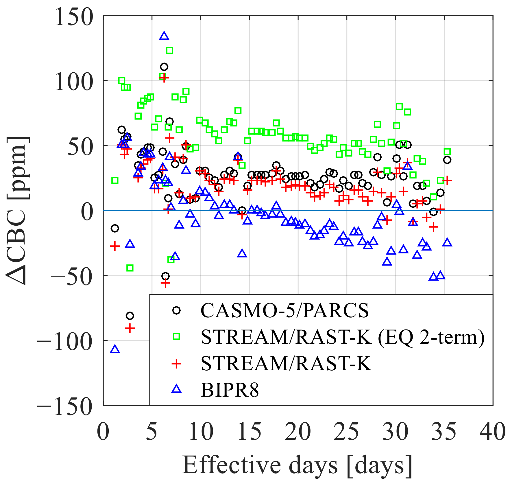
Figure 21 contains differences in terms of critical boron concentration with respect to the measurements. The BIPR8 results from reference [15] are also provided. A total of 76 depletion points are used for comparison. Average RMS differences in terms of boron concentrations are 32, 37, and 32 ppm in STREAM/RAST-K, CASMO-5/PARCS, and BIPR-8 calculations, respectively. Compared with previous VVER-1000 analysis [7], calculation results have comparable accuracy.
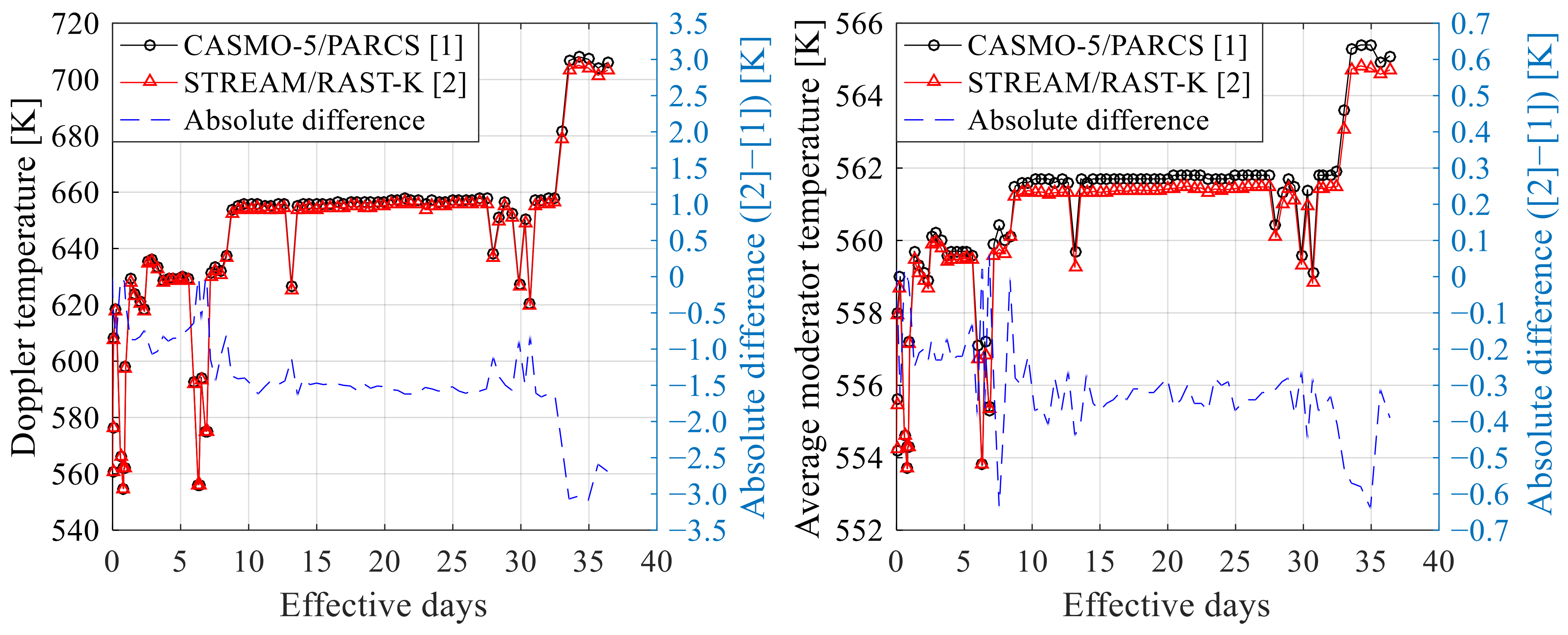
Figure 22 contains the comparison results of T/H parameters, Doppler temperature, and volume average moderator temperature. Same material properties are used in T/H feedback at PARCS and RAST-K calculations. STREAM/RAST-K and CASMO-5/PARCS present good agreement. Figure 23 presents the relative power difference of RAST-K with respect to the measurement [15] at 36.73 EFPDs. The relative differences are within ±2.46% and the RMS difference is 1.23%. Figure 24 contains the same information for the PARCS solution. Relative differences are within ±4.29%, and a RMS difference is 1.58%. As shown in these figures, an in-out tilt is observed in both codes. This effect may be related to the modeling of the radial reflector. The overestimation of the FA power at the core center from the two-step approach as compared to the measurement is consistent with the results of the 2D fresh core calculations shown in Section 3.2. In addition, to assess the effect of radial reflector model in terms of radial power distribution, a comparison is performed with 1D and 2D radial reflectors, as shown in Figure 23. In this calculation, group constants, ADFs, and CDFs of reflectors, are calculated by each reflector model: 1D and 2D cases use those from 1D and 2D reflector models, respectively. Only minor difference is reported.
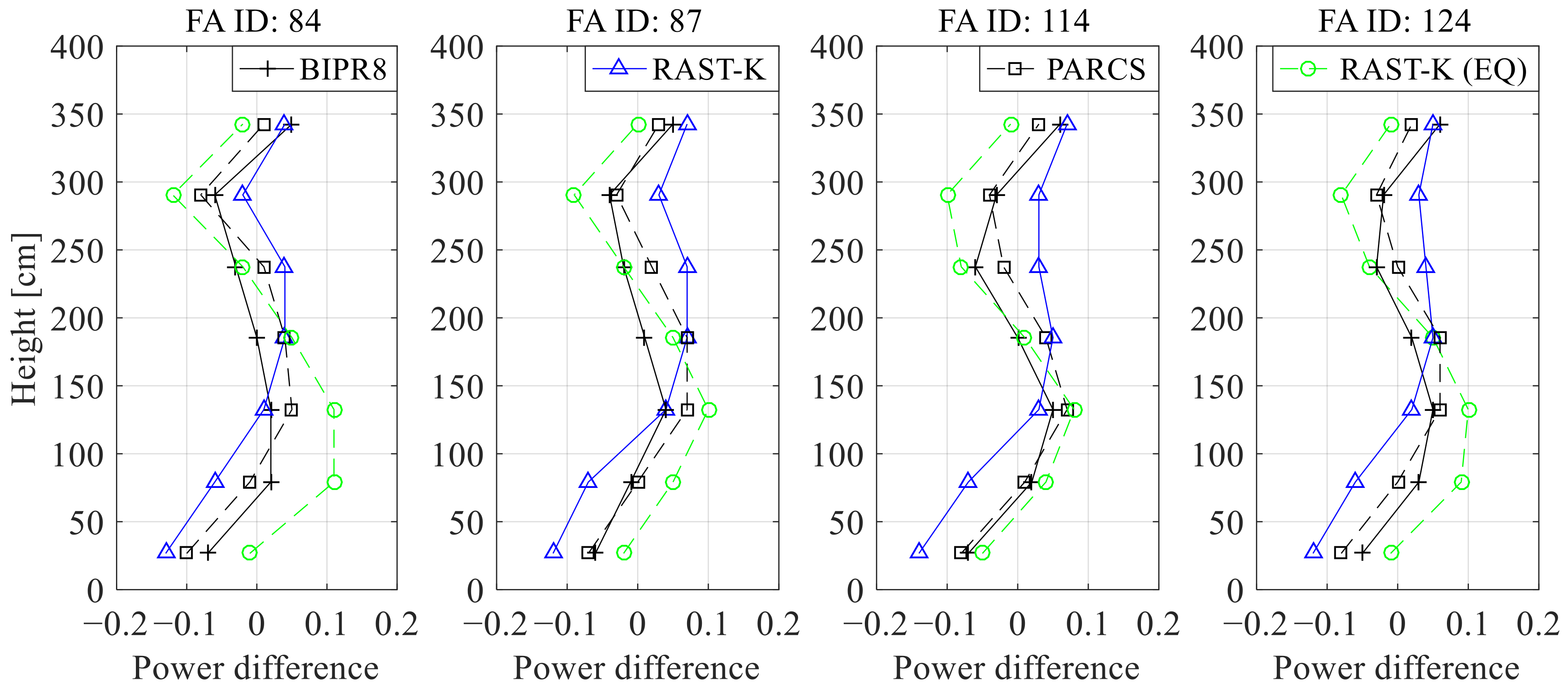
Figure 25 presents the axial power distribution of STREAM/RASTK, CASMO-5/PARCS, and BIPR8 compared with the measurements at 36.73 EFPDs. The normalized axial power for the measurements and BIPR8 solution are obtained from reference [15]. The location of the four FAs used for comparison is shown in Figure 10c. FA IDs are 84, 87, 114, and 124. As shown in the Figure 25, the various axial power profiles considered have large differences near the bottom reflector regions. Table 7 contains the RMS differences and RAST-K has slightly larger difference with respect to the measurements than BIPR8 or PARCS, which show similar performance. Using the same resonance model in STREAM and CASMO-5 tends to reduce this discrepancy.
6. Conclusions
This paper presents the analysis of the Rostov-II benchmark using conventional two-step approach code systems: CASMO-5/PARCS, and UNIST in-house code system STREAM/RAST-K. This paper covers the V&V of the calculation scheme of STREAM/RAST-K and CASMO-5/PARCS for VVERs, and generation of two conventional solutions for the Rostov-II benchmark. Serpent 2 is used for code-to-code comparison at the lattice and 2D core level, and 3D results of both deterministic models are compared to the steady state measurements of the Rostov-II benchmark.
The comprehensive set of calculations performed with STREAM/RAST-K and CASMO-5/PARCS at the FA, 2D, and 3D core levels have shown the good performances of those two conventional code systems. With respect to the measurements available in the Rostov-II benchmark, comparable accuracy (30 ppm difference in boron concentration, 2% assembly power) with BIPR8 is reported up to 36.73 EFPDs. The outcomes of the calculations reported in the paper showed that the modeling of the resonance self-shielding in the lattice code as well as the geometrical modeling of the reflector are key for an accurate solution (reducing the in-out power tilt). At the core simulator level, a fairly crude 1D reflector model appears to be enough.
In addition, the generated few-group constants by the lattice codes show good agreement compared to Serpent 2, by achieving 1% difference except for the diffusion coefficient (~1.5%). This difference has negligible effect on the radial power comparison, achieving assembly power difference within ±2.47% between STREAM/RAST-K and Serpent 2 in the 2D core model. Moreover, sensitivity study of resonance treatment is performed with PSM and EQ two-term. This study concludes that the PSM method has better agreement in terms of multiplication factor and CBC result with the measurement.
Overall, this paper provides detail calculation models and conditions used in STREAM/RAST-K and CASMO-5/PARCS, and accurate calculation solution for the Rostov-II benchmark with STREAM/RAST-K and CASMO-5/PARCS. As future work, the boron dilution transient will be performed by using STREAM/RAST-K and TRACE/PARCS.
Author Contributions
Conceptualization, M.H.; Resources, M.H., A.P., M.P. and H.F.; Software, J.J. and W.L.; Supervision, M.H. and D.L.; Validation, J.J. and W.L.; Visualization, J.J.; Writing—original draft, J.J.; Writing—review & editing, M.H., W.L., A.P., M.P., H.F. and D.L. All authors have read and agreed to the published version of the manuscript.
Funding
This work was supported by the National Research Foundation of Korea (NRF) grant funded by the Korea government (MSIT) (No. NRF-2017M2A8A2018595 and No. NRF-2019K1A3A1A14113717).
Institutional Review Board Statement
Not applicable.
Informed Consent Statement
Not applicable.
Conflicts of Interest
The authors declare no conflict of interest.
Abbreviations
| 1D | one-dimensional |
| 2D | two-dimensional |
| 3D | three-dimensional |
| ADF | assembly discontinuity factor |
| BOR | boron concentration |
| CDF | corner flux discontinuity factor |
| CMFD | coarse mesh finite difference |
| CR | control rod |
| CRAM | Chebyshev rational approximation method |
| DRI | distribution resonance integral |
| EFPD | effective full power day |
| FA | fuel assembly |
| HFP | hot full power |
| HZP | hot zero power |
| MAX | maximum |
| MIN | minimum |
| MOC | method of characteristics |
| NPP | nuclear power plant |
| PSM | point energy slowing-down method |
| PWR | pressurized water reactor |
| Q value | energy release per fission |
| RA | reflector assembly |
| RMS | root mean square |
| TFU | fuel temperature |
| TH1D | Simplified one-dimensional single channel thermal-hydraulic feedback |
| T/H | thermal-hydraulic |
| TPEN | Triangular-based polynomial expansion nodal method |
| TMO | moderator temperature |
| UNM | unified nodal method |
| VVER | Vodo-Vodyanoi Energetichesky Reactor |
| V&V | verification and validation |
| WT.% | weight percent |
Appendix A
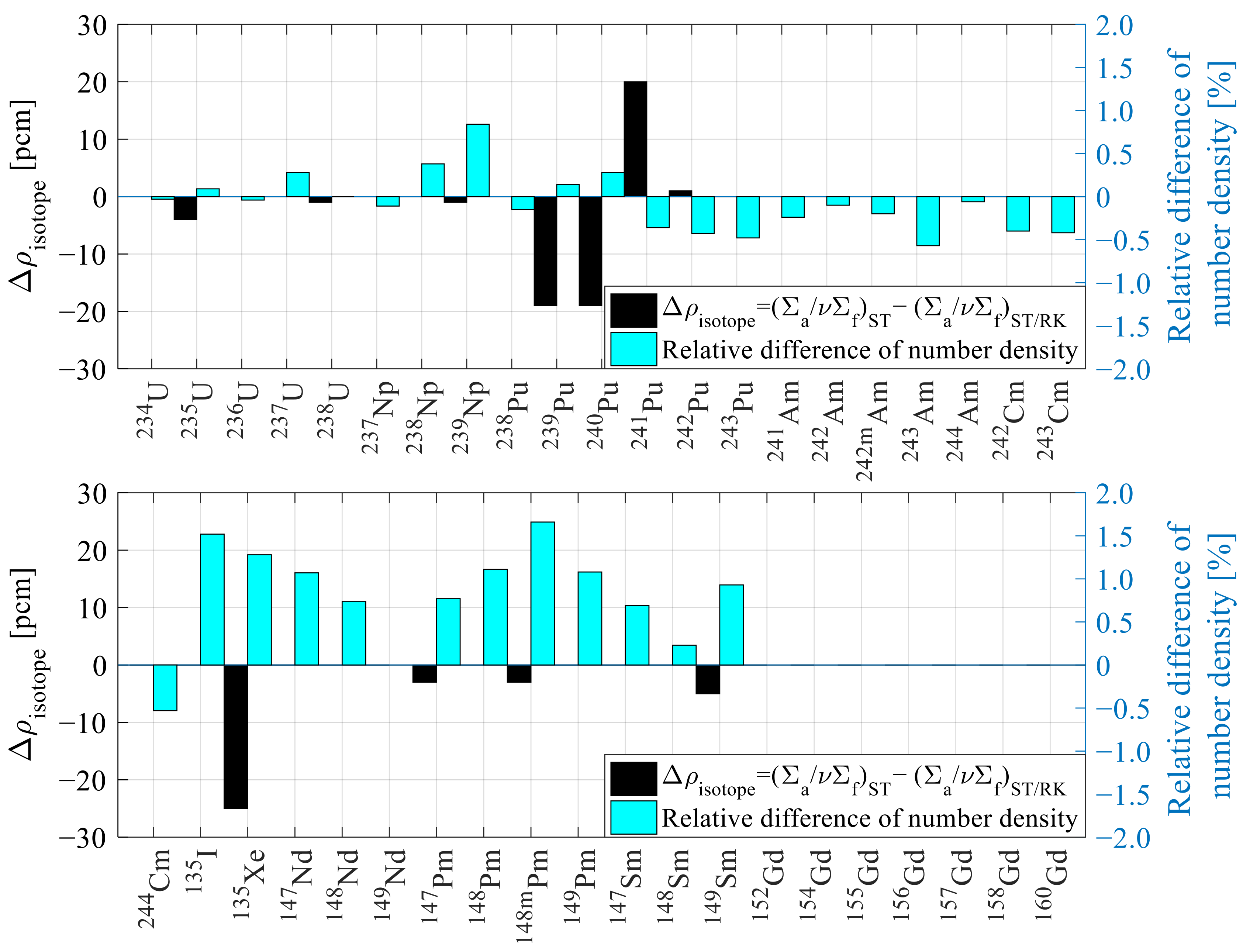
Table A1 contains the detail information of the multiplication factors in various calculation conditions. Sensitivity study of Pn-scattering order also contains in this table. Figure A1 contains the detail information of multiplication factor difference between STREAM and STREAM/RAST-K calculations. Calculation model is U22 FA which is one of Rostov-II FA model and comparison was performed at 20 MWd/kg. Although the differences of 135Xe and 239, 240, and 241Pu are larger than other isotopes, all differences are within ±30 pcm.

Table A1.
Multiplication factor in various calculation conditions.
| Parameter | Serpent 2 [A] | STREAM [B] | CASMO-5 [C] | ||||||
|---|---|---|---|---|---|---|---|---|---|
| 0th Order Pn-Scattering | 3rd Order Pn-Scattering | ||||||||
| Case | wt.% | keff | Std. a [pcm] | keff | Diff. b [pcm] | keff [C] | Diff. c [pcm] | keff [D] | Diff. d [pcm] |
| HZP, rod out | 1.3 | 0.92341 | 6 | 0.92290 | −51 | 0.92367 | 26 | 0.92342 | 1 |
| 2.2 | 1.10309 | 6 | 1.10261 | −48 | 1.10358 | 49 | 1.1033 | 21 | |
| 3.0 | 1.19464 | 5 | 1.19433 | −31 | 1.19537 | 73 | 1.19507 | 43 | |
| 3.6 | 1.24259 | 5 | 1.24223 | −36 | 1.24328 | 69 | 1.24297 | 38 | |
| 4.0 | 1.26815 | 5 | 1.26784 | −31 | 1.26888 | 73 | 1.26855 | 40 | |
| HFP, rod out | 1.3 | 0.91541 | 5 | 0.91476 | −65 | 0.91521 | −20 | 0.91495 | −46 |
| 2.2 | 1.09374 | 6 | 1.09313 | −61 | 1.0937 | −4 | 1.09341 | −33 | |
| 3.0 | 1.18483 | 6 | 1.18425 | −58 | 1.18486 | 3 | 1.18455 | −28 | |
| 3.6 | 1.23253 | 5 | 1.23188 | −65 | 1.23249 | −4 | 1.23216 | −37 | |
| 4.0 | 1.25802 | 5 | 1.25734 | −68 | 1.25793 | −9 | 1.25759 | −43 | |
| HFP, rod in, B4C | 1.3 | 0.64338 | 10 | 0.64516 | 178 | 0.64795 | 457 | 0.64525 | 187 |
| 2.2 | 0.80077 | 9 | 0.80319 | 242 | 0.80604 | 527 | 0.80307 | 230 | |
| 3.0 | 0.88988 | 9 | 0.89290 | 302 | 0.89568 | 580 | 0.89266 | 278 | |
| 3.6 | 0.94005 | 8 | 0.94307 | 302 | 0.94579 | 574 | 0.94277 | 272 | |
| 4.0 | 0.96761 | 8 | 0.97103 | 342 | 0.97368 | 607 | 0.97067 | 306 | |
| HFP, rod in, Dy2O3-TiO2 | 1.3 | 0.69547 | 9 | 0.69298 | −249 | 0.69739 | 192 | 0.69539 | −8 |
| 2.2 | 0.86467 | 10 | 0.86162 | −305 | 0.8673 | 263 | 0.86523 | 56 | |
| 3.0 | 0.95989 | 8 | 0.95636 | −353 | 0.96282 | 293 | 0.96081 | 92 | |
| 3.6 | 1.01280 | 8 | 1.00891 | −389 | 1.01581 | 301 | 1.01385 | 105 | |
| 4.0 | 1.04193 | 7 | 1.03802 | −391 | 1.04514 | 321 | 1.04322 | 129 | |
a. standard deviation of a Monte Carlo simulation; b. difference calculated by [B] − [A]; c. difference calculated by [C] − [A]; d. difference calculated by [D] − [A].
Figure A1.
Calculation difference between STREAM and STREAM/RAST-K (calculation model: U22, burnup: 20 MWd/kg).
Figure A1.
Calculation difference between STREAM and STREAM/RAST-K (calculation model: U22, burnup: 20 MWd/kg).

References
- The VVER Today, ROSATOM. Available online: https://rosatom.ru/upload/iblock/0be/0be1220af25741375138ecd1afb18743.pdf (accessed on 31 May 2018).
- Current Status of Russian Nuclear Power Development and Cooperation with Europe: The Issue of Human Resource Development Rosatom Technical Academy. Available online: https://enen.eu/wp-content/uploads/2019/08/13-artisiuk_01_03_18_brussel.pdf (accessed on 1 March 2018).
- Russian Nuclear Power 2018, Bellona, P17. Available online: https://network.bellona.org/content/uploads/sites/2/2018/08/Russian-Nuclear-Power-2018.pdf (accessed on 2 August 2018).
- Sahlberg, V. Calculating V-1000 Core Model with Serpent 2—HEXTRAN Code Sequence. In Proceedings of the M&C 2017, Jeju, Korea, 16–20 April 2017. [Google Scholar]
- Vojackova, J.; Novotny, F.; Katovsky, K. Safety analyses of reactor VVER 1000. In Proceedings of the International Youth Nuclear Congress 2016, IYNC2016, Hangzhou, China, 24–30 July 2016. [Google Scholar]
- Bznuni, S.; Amirjanyan, A.; Baghdasaryan, N.; Baiocco, G.; Petruzzi, A.; Kohut, P.; Ramsey, J. Comparative analysis of WWER-440 Reactor core with PARCS/Helios and PARCS/Serpent Codes. In Proceedings of the IAEA Conference on Topical Issues of Nuclear Safety of Nuclear Power Plants: Safety Demonstration of Advanced Water-Cooled Nuclear Power Plants, Vienna, Austria, 6–9 June 2017; Available online: https://www-pub.iaea.org/MTCD/Publications/PDF/STIPUB1829_volOneWeb.pdf (accessed on 6 June 2017).
- Ferrer, R.; Bahadir, T. Validation of new CMS5-VVER nuclear data library using critical experiments and X2 full-core benchmark. Kerntechnik 2020, 85, 205–212. [Google Scholar] [CrossRef]
- Grundmarin, U.; Kiem, S.; Ko7menkov, Y.; Minag, S.; Rohde, U.; Weiss, F.-P. Transient Simulations in Vver-1000—Comparison between Dyn3d-Athlet and Dyn3d-Relap5, Gesellschaft für Anlagenund Reaktorsicherheit (GRS) mbH, Forschungszentrum Rossendorf, P.O.Box 510119, D-01314 Dresden. 2004. Available online: https://inis.iaea.org/collection/NCLCollectionStore/_Public/36/107/36107104.pdf?r=1&r=1 (accessed on 2 August 2004).
- Hegyi, G.; Keresztúri, A.; Trosztel, I.; Elter, Z. ATHLET/KIKO3D results of the OECD/NEA benchmark for coupled codes on KALININ-3 NPP measured data. In Proceedings of the NENE, Portoroz, Slovenia, 8–11 September 2014. [Google Scholar]
- Avramova, M.; Ivanov, K.; Velkov, K.; Nikonov, S.; Gordienko, P.; Shumskiy, B.; Kavun, O. Benchmark on Reactivity Compensation of Boron Dilution by Stepwise Insertion of Control Rod Cluster into the VVER-1000 Core, Version 1.5; OECD Nuclear Energy Agency: Paris, France, March 2020.
- Ojinnaka, C.A.S.; Zimin, V.G.; Strashnykh, V.P.; Nikonov, S.P. Analysis of the Kalinin-3 coolant transient benchmark by SKETCH-N/SKAZKA code system. Ann. Nucl. Energy 2020, 147, 107716. [Google Scholar] [CrossRef]
- Weiss, F.P.; Mittag, S. Validation of Coupled Neutron-Kinetic/Thermal-Hydraulic Codes against Transients Measured in VVER Reactors. Phare SRR-1/95: Final Technical Report FZR/SRR195/FIN2.1; Forschungszentrum Rossendorf: Brussels, Belgium, 2000. [Google Scholar]
- Mittag, S.; Grundmann, U.; Kliem, S.; Kozmenkov, Y.; Rindelhardt, U.; Rohde, U.; Weiss, F.-P.; Langenbuch, S.; Krzykacz-Hausmann, B.; Schmidt, K.-D.; et al. Validation of Coupled Neutronic/Thermal-Hydraulic Codes for VVER Reactors FINAL Report; FZR-408; Forschungszentrum Rossendorf e.V. (FZR): Dresden, Germany, 2004. [Google Scholar]
- AER Benchmark Book; Atomic Energy Research (AER): Budapest, Hungary, 1999; Available online: http://aerbench.kfki.hu (accessed on 15 April 1999).
- Gordienko, P.; Shumsky, B. Rostov-2. Neutron-physical modeling of the initial state and updating data to prepare constants. In Proceedings of the 2nd Rostov-2 Workshop, Garching, Germany, 20 November 2020. [Google Scholar]
- Gordienko, V.P.; Kiryukhin, K.P.; Shcherbakov, A.A. Benchmark calculation AER VVER-1000—ETE using BIPR8. J. Phys. Conf. Ser. 2018, 1133, 012043. [Google Scholar] [CrossRef]
- Kotsarev, A.; Lizorkin, M.; Shumskiy, B. The results of the certification of the code ATHLET/BIPR-VVER version 1.0. In Proceedings of the 29th Symposium of AER on VVER Reactor Physics and Reactor Safety, Energoland, Mochovce NPP, Kalná nad Hronom, Slovakia, 14–18 October 2019. [Google Scholar]
- Gado, J. BIPR Program for the Calculation of the VVER-440 Type Nuclear Power Reactor Calculations; KFKI-1978-72; Kozponti Fizikai Kutato Intezet: Budapest, Hungary, 1978. [Google Scholar]
- CASMO-5 a Fuel Assembly Burnup Program User’s Manual; Proprietary SSP-07/431; Studsvik Scandpower, Inc.: Waltham, MA, USA, 2015.
- Downar, T.; Xu, Y.; Seker, V.; Hudson, N. PARCS NRC—v3.3.1 Volume I: Input Manual; RES/U.S. NRC: Rockville, MD, USA, 2018. [Google Scholar]
- Choi, S.; Kim, W.; Choe, J.; Lee, W.; Kim, H.; Ebiwonjumi, B.; Jeong, E.; Lee, H.; Yun, D.; Lee, D. Development of High-Fidelity Neutron Transport Code STREAM. Comput. Phys. Commun. 2021, 264, 107915. [Google Scholar] [CrossRef]
- Park, J.; Jang, J.; Kim, H.; Choe, J.; Yun, D.; Zhang, P.; Cherezov, A.; Lee, D. RAST-K v2- Three Dimensional Nodal Diffusion Code for Pressurized Water Reactor Core Analysis. Energies 2020, 13, 6324. [Google Scholar] [CrossRef]
- Cho, J.Y.; Kim, C.H. Higher Order Polynominal Expansion Nodal Method for Hexagonal Core Neutronics Analysis. Ann. Nucl. Energy 1998, 25, 1021–1031. [Google Scholar] [CrossRef]
- Jang, J.; Quoc, T.T.; Dzianisau, S.; Lee, W.; Lee, D. Verification of RAST-K hexagonal analysis module with SNR and VVER-440 benchmarks. In Proceedings of the KNS Winter Meeting, Online, 16–18 December 2020. [Google Scholar]
- Jang, J.; Chezerov, A.; Jo, Y.; Tran, T.Q.; Dzianisau, S.; Lee, W.; Park, J.; Lee, D. Verification of RAST-K hexagonal transient solver with OCED/NEA benchmark problem of KALININ-3 NPP. In Proceedings of the KNS Winter Meeting, Online, 16–18 December 2020. [Google Scholar]
- Papadionysiou, M.; Kim, S.; Hursin, M.; Vasiliev, A.; Ferroukhi, H.; Pautz, A.; Joo, H.G. Assessment of nTRACER and PARCS Performance for VVER Configurations. Nucl. Sci. Eng. 2020, 194, 1056–1066. [Google Scholar] [CrossRef]
- Choe, J.; Choi, S.; Zhang, P.; Park, J.; Kim, W.; Shin, H.C.; Lee, H.S.; Jung, J.; Lee, D. Verification and Validation of STREAM/RAST-K for PWR Analysis. Nucl. Eng. Technol. 2019, 51, 356–368. [Google Scholar] [CrossRef]
- Jang, J.; Choe, J.; Choi, S.; Park, J.; Lemaire, M.; Lee, D.; Shin, H.C. Westinghouse 2-loop Plant Loading Pattern Optimization for Last Few Cycles Before Shutdown. In Proceedings of the M&C 2019, Portland, OR, USA, 25–29 August 2019. [Google Scholar]
- Jang, J.; Choe, J.; Choi, S.; Lemaire, M.; Lee, D.; Shin, H.C. Conceptual Design of Long-cycle Boron-free Small Modular Pressurized Water Reactor with Control Rod Operation. Int. J. Energy Res. 2020, 44, 6463–6482. [Google Scholar] [CrossRef]
- Jang, J.; Choe, J.; Choi, S.; Lee, H.; Ebiwonjumi, B.; Shin, H.C.; Lee, D. Boron-free SMPWR Analysis with MCS and STREAM codes. In Proceedings of the RPHA17, Chengdu, China, 24–25 August 2017. [Google Scholar]
- Choi, S.; Lee, C.; Lee, D. Resonance Treatment Using Pin-Based Pointwise Energy Slowing-Down Method. J. Comput. Phys. 2017, 330, 134–155. [Google Scholar] [CrossRef] [Green Version]
- Choi, S.; Choe, J.; Jang, J.; Lee, D. Extension of PSM for Ring-Type Burnable Absorber Containing Resonant Nuclides. In Proceedings of the RPHA17, Chengdu, China, 24–25 August 2017. [Google Scholar]
- Choi, S.; Choe, J.; Nguyen, K.; Lee, W.; Kim, W.; Kim, H.; Ebiwonjumi, B.; Jeong, E.; Kim, K.; Lee, D. Developments of STREAM [ppt file], UNIST. 2020. Available online: https://drive.google.com/file/d/1O0sfSxcg5DeNOqFSOHkm6TGV47WwoAif/view (accessed on 31 May 2018).
- Chadwick, M.; Obložinský, P.; Herman, M.; Greene, N.; McKnight, R.; Smith, D.; Young, P.; MacFarlane, R.; Hale, G.; Frankle, S.; et al. ENDF/B-VII.0: Next Generation Evaluated Nuclear Data Library for Nuclear Science and Technology. Nucl. Data Sheets 2006, 107, 2931–3060. [Google Scholar] [CrossRef] [Green Version]
- Croff, A.G. A User’s Manual for the ORIGEN2 Computer Code, Oak Ridge National Laboratory, ORNL/TM-7175. 1980. Available online: https://inis.iaea.org/collection/NCLCollectionStore/_Public/11/560/11560149.pdf (accessed on 31 May 2018).
- Du, X.; Choe, J.; Choi, S.; Cherezov, A.; Lee, W.; Quoc, T.T.; Park, J.; Lee, D. Recent Progress on Fast Reactor Analysis in UNIST CORE Laboratory. In Proceedings of the KNS Spring Meeting, Jeju, Korea, 22–24 May 2019. [Google Scholar]
- Du, X.; Choe, J.; Quoc, T.T.; Lee, D. Neutronic Simulation of China Experimental Fast Reactor Start-up Test. Part I: SARAX Code Deterministic Calculation. Ann. Nucl. Energy 2020, 136, 107046. [Google Scholar] [CrossRef]
- Jang, J.; Ebiwonjumi, B.; Kim, W.; Park, J.; Lee, D. Verification and Validation of Isotope Inventory Prediction for Back-End Cycle Management by Two-Step Method. Nucl. Eng. Technol. 2021, 53, 2104–2125. [Google Scholar] [CrossRef]
- Ward, A.; Xu, Y.; Downar, T. GenPMAXS—v6.2: Code for Generating the PARCS Cross Section Interface File PMAXS; University of Michigan: Ann Arbor, MI, USA, 2016. [Google Scholar]
- Downar, T.; Ward, A.; Xu, Y.; Seker, V.; Hudson, N.; Barber, D.; Roth, G. PARCS, NRC-v3.3.0 Release, Volume II: User’s Guide; University of Michigan: Ann Arbor, MI, USA, 2018. [Google Scholar]
- Leppänen, J.; Pusa, M.; Viitanen, T.; Valtavirta, V.; Kaltiaisenaho, T. The Serpent Monte Carlo code: Status, development and applications in 2013. Ann. Nucl. Energy 2013, 82, 142–150. [Google Scholar] [CrossRef]
- Leppänen, J. Greetings from the Serpent developer team & current status and future plans for Serpent 2. In Proceedings of the 8th International Serpent UGM, Espoo, Finland, 29 May–1 June 2018. [Google Scholar]
- Bilodid, Y.; Fridman, E.; Lötsch, T. X2 VVER-1000 benchmark revision: Fresh HZP core state and the reference Monte Carlo solution. Ann. Nucl. Energy 2020, 144, 107558. [Google Scholar] [CrossRef]
- Jo, Y.; Hursin, M.; Lee, D.; Ferroukhi, H.; Pautz, A. Analysis of simplified BWR full core with serpent-2/simulate-3 hybrid stochastic/deterministic code. Ann. Nucl. Energy 2018, 111, 141–151. [Google Scholar] [CrossRef]
- Hursin, M.; Vasiliev, A.; Pautz, A. Comparison of SERPENT and CASMO-5M for Pressurized Water Reactors Models. In Proceedings of the M&C 2013, Sun Valley, ID, USA, 5–9 May 2013. [Google Scholar]
- IAEA Power Reactor Information system, IAEA. Available online: https://pris.iaea.org/PRIS/CountryStatistics/ReactorDetails.aspx?current=505 (accessed on 31 May 2018).
- Bahadir, T.; Geogieva, E. ‘FULLCORE’ and ‘MIDICORE’ VVER-1000 Benchmark Evaluations with Studsvik’s CMS5-VVER Codes. In Proceedings of the 28th Symposium of AER on VVER Reactor Physics and Reactor Safety, Olomouc, Czechia, 8–12 October 2018. [Google Scholar]
- Usheva, K.I.; Kuten, S.A.; Khruschinsky, A.A.; Babichev, L.F. Generation of XS library for the reflector of VVER reactor core using Monte Carlo code Serpent. IOP Conf. Ser. J. Phys. Conf. Ser. 2017, 781, 012029. [Google Scholar] [CrossRef] [Green Version]
- Ferrer, R.; Hykes, J.; Rohodes, J., III; Kropaczek, D. CASMO-5 a Fuel Assembly Burnup Program Methodology Manual; Studsvik Scandpower, Inc.: Waltham, MA, USA, 2015. [Google Scholar]
- Rhodes, J. ENDF/B-VII.0 586 Group Neutron Data Library for CASMO-5 and CASMO-5M; SSP-07/402 Rev 5; Studsvik: Waltham, MA, USA, 2009. [Google Scholar]
- Tuominen, R. New energy deposition treatment in Serpent 2. In Proceedings of the Serpent User Group Meeting, Espoo, Finland, 29 May–1 June 2018; Available online: http://montecarlo.vtt.fi/mtg/2018_Espoo/Tuominen1.pdf (accessed on 31 May 2018).
- Rhodes, J.; Smith, K.; Xu, Z. CASMO-5 Energy Release per Fission Model, Studsvik Scandpower Inc. Available online: https://www.studsvik.com/SharepointFiles/CASMO-5%20Energy%20Release%20per%20Fission%20Model.pdf (accessed on 31 May 2018).
- Park, J.; Kim, W.; Choi, S.; Lee, H.; Lee, D. Comparative Analysis of VERA Depletion Problems. In Proceedings of the Transactions of the Korean Nuclear Society Autumn Meeting, Gyeongju, Korea, 27–28 October 2016; Available online: https://www.kns.org/files/pre_paper/36/16A-113%EB%B0%95%EC%A7%84%EC%88%98.pdf (accessed on 27 October 2016).
- Park, J.; Lee, D. Consistent Code-to-Code Comparison of Pin-cell Depletion Benchmark Suite. In Proceedings of the 6th International Serpent User Group Meeting, Milan, Italy, 26–29 September 2016; Available online: http://montecarlo.vtt.fi/mtg/2016_Milan/Park.pdf (accessed on 27 September 2016).
- Kang, S.; Cole, A.G.; Andrew, T.G.; Yuxuan, L.; Scott, P. Development of the multigroup cross section library for the CASL neutronics simulator MPACT: Verification. Ann. Nucl. Energy 2019, 132, 1–23. [Google Scholar]
- Choi, S.; Smith, K.S.; Kim, H.; Tak, T.; Lee, D. On the diffusion coefficient calculation in two-step light water reactor core analysis. J. Nucl. Sci. Technol. 2017, 54, 705–715. [Google Scholar] [CrossRef]
- Herman, B.R.; Forget, B.; Smith, K. Improved Diffusion Coefficients Generated from Monte Carlo Codes. In Proceedings of the M&C 2013, Sun Valley, ID, USA, 5–9 May 2013. [Google Scholar]
- Fridman, E.; Leppänen, J.; Wemple, C. An Updated Approach to Calculation of Diffusion Coefficients. In Proceedings of the Serpent International User Group Meeting, Berkeley, CA, USA, 6–8 November 2013; Available online: http://montecarlo.vtt.fi/mtg/2016_Milan/Fridman1.pdf (accessed on 31 May 2018).
- Kim, S.; Joo, G.H. nTRACER Solutions of the Two-Dimensional VVER Benchmark Problems. In Proceedings of the Transactions of the Korean Nuclear Society Virtual Spring Meeting, Virtual, 9–10 July 2020. [Google Scholar]
- Stamm’ler, R.J.J.; Abbate, M.J. Methods of Steady-State Reactor Physics in Nuclear Design; Academic Press: London, UK, 1983. [Google Scholar]
Figure 1.
Flowchart of STREAM/RAST-K and CASMO-5/PARCS code system.

Figure 2.
Radial layouts of five different Rostov-II fuel assemblies.

Figure 3.
FA modeling approximation.

Figure 4.
Differences between nominal models and approximated models with Serpent 2.

Figure 5.
Radial layout of 1D radial reflector model.

Figure 6.
Radial layout of 2D radial reflector model.

Figure 7.
Radial layout of Rostov-II nominal radial reflector model.

Figure 8.
Composition of axial reflectors.

Figure 9.
Radial layout of Rostov-II reactor.

Figure 10.
Axial composition of simplified control rod and measured fuel assembly positions.

Figure 11.
Multiplication factors of STREAM and CASMO-5 in various simulation conditions.

Figure 12.
Capture cross section of 162Dy and 10B.

Figure 13.
Evolution of k-inf discrepancies during depletion calculations. Reference is Serpent 2.

Figure 14.
Comparison of radial power distribution.

Figure 15.
STREAM few-group constants compared with Serpent 2 and CASMO-5.

Figure 16.
Radial layout of the nominal and simplified reflector model.

Figure 17.
Radial power distribution of Serpent 2, STREAM and CASMO-5.

Figure 18.
Pin power difference with different resonance treatment.

Figure 19.
Radial power distribution of Serpent 2 with different reflector models.

Figure 20.
Radial power differences of PARCS with respect to CASMO-5 for different reflector models.
Figure 20.
Radial power differences of PARCS with respect to CASMO-5 for different reflector models.

Figure 21.
Absolute difference of boron concentration with measurement.

Figure 22.
T/H Feedback—inlet, flowrate, fuel temperature (doppler).

Figure 23.
Relative radial power difference of RAST-K compared with measurement.

Figure 24.
Relative radial power difference of PARCS compared with measurement.

Figure 25.
Axial power difference at 36.73 effective days.

Table 1.
Specification of Rostov-II.
| Parameter | Value | Unit |
|---|---|---|
| Nominal thermal power | 3000 | MW |
| Fuel assembly type | TBC-2M | |
| Fuel assembly pitch | 23.4 | cm |
| Pin pitch | 1.275 | cm |
| Number of fuel assemblies | 163 | |
| Active core height | 370 | cm |
Table 2.
Specification of Rostov-II fuel assemblies.
| FA Type | Number of Fuel Pins/Enrichment (wt.% 235U) | Number of Gadolinia Pins (wt.% Gd2O3/235U) | Number of Fuel Assembly in the Core |
|---|---|---|---|
| U13 | 312/1.3 | - | 48 |
| U22 | 312/2.2 | - | 42 |
| U30Y9 | 303/3.0 | 9 (8.0/2.4) | 37 |
| U39A9 | 243/4.0, 60/3.6 | 9 (5.0/3.3) | 24 |
| U39B6 | 240/4.0, 66/3.6 | 6 (5.0/3.3) | 12 |
Table 3.
Calculation condition for sensitivity study.
| Parameter | Value | |
|---|---|---|
| Fuel temperature | 900 K | |
| Moderator temperature | 600 K | |
| Boron concentration | 1000 ppm | |
| Calculated burnup range | 0–50 MWd/kg | |
| Number of depletion steps | 39 | |
| Number of fuel rod rings | 5 rings for UO2 fuel pin 10 rings for Gadolinia pin | |
| Particle histories in Serpent 2 | Histories/cycle | 400,000 |
| Inactive cycles | 20 | |
| Active cycles | 100 | |
| MOC Ray condition in STREAM | Ray spacing | 0.03 cm |
| Polar angles in π | 6 | |
| Azimuthal angles in 2π | 96 | |
| MOC Ray condition in CASMO-5 | Ray spacing | 0.05 cm |
| Polar angles in π | 8 | |
| Azimuthal angles in 2π | 64 | |
Table 4.
Multiplication factor of three difference test cases.
| Case (TFU a, TMO b, BOR c) | Serpent 2 | STREAM | CASMO-5 | ||
|---|---|---|---|---|---|
| keff | keff | Diff. [pcm] | keff | Diff. [pcm] | |
| CASE01 (900 K a, 600 K b, 1000 ppm c) | 1.01707 ± 0.00001 | 1.01726 | 19 ± 1 | 1.01796 | 89 ± 1 |
| CASE02 (900 K a, 600 K b, 0 ppm c) | 1.14575 ± 0.00001 | 1.14538 | −37 ± 1 | 1.14579 | 4 ± 1 |
| CASE03 (600 K a, 600 K b, 0 ppm c) | 1.15543 ± 0.00001 | 1.15534 | −9 ± 1 | 1.15566 | 23 ± 1 |
a is fuel temperature; b is moderator temperature; c is boron concentration.
Table 5.
Relative power difference compared with Serpent 2.
| Code | CASMO-5 | STREAM | ||
|---|---|---|---|---|
| Parameter | Pin Power | FA Power | Pin Power | FA Power |
| Minimum | −3.08 | −3.11 | −1.99 | −1.30 |
| Maximum | 2.45 | 3.12 | 2.25 | 1.66 |
| RMS | 1.07 | 1.62 | 0.70 | 0.70 |
Table 6.
Comparison of three different code systems for the 2D Rostov-II model.
| Code | Reflector Type | keff | Difference a [pcm] | Relative Power Difference [%] | ||
|---|---|---|---|---|---|---|
| Min | Max | RMS | ||||
| Serpent 2 | Nominal reflector | 1.01749 ± 0.00002 | - | - | - | - |
| CASMO-5/PARCS | 1D | 1.01822 | 73 ± 2 | −1.93 | 1.85 | 0.97 |
| 2D | 1.01839 | 90 ± 2 | −1.60 | 1.71 | 0.87 | |
| Core | 1.01820 | 71 ± 2 | −1.61 | 1.62 | 0.83 | |
| STREAM/RAST-K | 1D | 1.01732 | −17 ± 2 | −2.47 | 2.21 | 1.23 |
| 2D | 1.01767 | 18 ± 2 | −2.04 | 1.78 | 1.07 | |
| Core | 1.01786 | 37 ± 2 | −2.29 | 1.50 | 0.95 | |
a reference is Serpent 2.
Table 7.
Relative RMS difference of axial power profile.
| FA ID | 84 | 87 | 114 | 124 |
|---|---|---|---|---|
| BIPR8 | 5.30% | 5.36% | 6.04% | 5.94% |
| RAST-K | 7.49% | 8.68% | 8.82% | 7.77% |
| PARCS | 5.52% | 5.20% | 5.03% | 5.02% |
| RAST-K (EQ) a | 5.77% | 4.56% | 4.96% | 4.84% |
a EQ is the cross section generated with EQ 2-term method in lattice code.
Publisher’s Note: MDPI stays neutral with regard to jurisdictional claims in published maps and institutional affiliations. |
© 2022 by the authors. Licensee MDPI, Basel, Switzerland. This article is an open access article distributed under the terms and conditions of the Creative Commons Attribution (CC BY) license (https://creativecommons.org/licenses/by/4.0/).
Share and Cite
MDPI and ACS Style
Jang, J.; Hursin, M.; Lee, W.; Pautz, A.; Papadionysiou, M.; Ferroukhi, H.; Lee, D. Analysis of Rostov-II Benchmark Using Conventional Two-Step Code Systems. Energies 2022, 15, 3318. https://0-doi-org.brum.beds.ac.uk/10.3390/en15093318
AMA Style
Jang J, Hursin M, Lee W, Pautz A, Papadionysiou M, Ferroukhi H, Lee D. Analysis of Rostov-II Benchmark Using Conventional Two-Step Code Systems. Energies. 2022; 15(9):3318. https://0-doi-org.brum.beds.ac.uk/10.3390/en15093318
Chicago/Turabian StyleJang, Jaerim, Mathieu Hursin, Woonghee Lee, Andreas Pautz, Marianna Papadionysiou, Hakim Ferroukhi, and Deokjung Lee. 2022. "Analysis of Rostov-II Benchmark Using Conventional Two-Step Code Systems" Energies 15, no. 9: 3318. https://0-doi-org.brum.beds.ac.uk/10.3390/en15093318
Note that from the first issue of 2016, this journal uses article numbers instead of page numbers. See further details here.