Three-Phase Unbalance Improvement for Distribution Systems Based on the Particle Swarm Current Injection Algorithm

Abstract

The aim of this study is to improve the three-phase unbalanced voltage at the secondary side of a distribution transformer. The proposed method involves compensation sources injecting three different single-phase currents into the connected point of a grid. The computations of optimal single-phase currents are performed using the circuit analysis method and particle swarm optimization algorithm. An unbalanced three-phase power distribution system model is constructed, including a transformer Δ–Δ connection, V–V connection, load balance, load unbalance combination, and three single-phase compensation current sources. The results show that the voltage unbalance rate of the electricity user side is improved to less than 1%, and the three-phase total compensation apparent power is approximately 0 VA. In the future, the application of the model as an auxiliary service could be achieved by adding an energy storage system.

1. Introduction

Voltage and current unbalances are common throughout electricity distribution networks. The factors causing unbalances can be separated into normal factors and abnormal factors. Normal factors include single-phase loads and three-phase transformer banks with open wye (Y–Y) and open delta (V–V) connections. Abnormal factors are caused by critical damage situations for systems and equipment [1,2]. Even in symmetric structures, with proper system design and suitable equipment and device installation, the diversity in different single phases can cause an unbalanced load and neutral current at any time [3].

The impacts of unbalances include efficiency reduction, damage increase, and malfunction accidents. For example, the voltage unbalance, containing zero- and negative-phase sequence voltages, can cause three-phase induction motors to reduce their torque output and increase losses. Furthermore, the voltage unbalance, containing a zero-sequence current, flows into the neutral line and can trip the low energy overcurrent (LCO) protective relay or zero-sequence relay, as well as increase the neutral-to-ground voltage [3]. The unbalanced voltage can limit the operation of distributed generation systems [4].

From the literature survey, the available methods for solving unbalance problems can be separated into reconfiguration in the design stage and the control of power flows in the operation stage. For reconfiguration methods in the design stage, the average load of each phase distribution is evaluated by long-term profiles, then the optimal connection of the feeder, transformer, or bus is determined. A particle swarm optimization (PSO) algorithm was applied to rearrange the phase connection of distribution transformers with the aim of minimizing the neutral current [3]. A mixed-integer programming model with binary variables solved the line-switching statuses and tap positions [4]. In general, these methods are automated, but failure may occur because of frequent load variations.

For power flow control methods in the operation stage, several power electronic devices have been proposed that smoothly control the power flow, such as an active power filter (APF), distribution static compensator (DSTATCOM), auto-balancing transformer, electric spring circuit, and soft open points. These approaches can improve unbalance issues caused by load variations in real time. APF and DSTATCOM can be used for the compensation of unbalanced loads in distribution systems. The principle of load balancing is achieved by balancing the source reference current [5,6]. An auto-balancing transformer, based on multilevel converters, can prevent voltage and current unbalances arising on the primary side system [7]. A three-phase electric spring circuit in series with noncritical loads can be used to reduce the power imbalance of electric power infrastructures in buildings [8]. A novel method, soft open points (SOPs), can connect different feeders to mitigate the three-phase unbalance of the upper-level grid [9,10,11,12]. Similar to SOPs, a rail power conditioner (RPC) can mitigate the unbalance caused by two single phases [13].

To summarize the above techniques, APF and DSTATCOM can balance the current, but the voltage may still be unbalanced if the source is connected to an unbalanced transformer. Power electronic transformers do not have a capacity as high as conventional transformers. Furthermore, the electric spring requires noncritical loads and it limits the applications of power flow control methods. SOPs appear useful but must be installed in the switch of the feeder. Hence, existing solutions for unbalance issues still have limitations.

Therefore, this study proposes a method that produces three single-phase currents to eliminate the unbalance component by steady control. This method is different to APF and DSTATCOM, which are based on instantaneous control, such as proportional–integral–derivative (PID) or fuzzy controller.

The rest of this paper is organized as follows. First, the simulation circuit model is introduced and worst-case unbalance situations are presented. Second, the compensation source model is designed and the PSO algorithm is implemented to provide a solution for each unbalance situation. The responses of varying loads and releasing the constraint are then analyzed and discussed.

2. Measurement of Unbalances

The definitions, approaches, and parameters of voltage unbalances in various fields are not consistent. There are some standards and regulations for definitions of voltage unbalances, such as IEC 34-1 (1983), NEMA MG1-1993, IEEE Std. 141-1993, IEEE Std. 936-1987, IEEE Std. 1159-2009, and IEC 1000-2-1/2. Despite the use of unground three-phase systems, for ground three-phase systems (i.e., $d_0\%$ ≠ 0), the $d_2\%$ and two-approximation equations are suggested to avoid misjudgment in evaluating voltage unbalance conditions [1].

The phase voltage unbalance (VU%) based on IEEE Std. 141-1993 is defined as the ratio of the maximum deviation of the phase voltage to the average phase voltage [14]. The voltage unbalance factor (VUF) describes the unbalance in the magnitudes and phase displacements of the sequence components, and is known as the “true definition” of the voltage unbalance [1], shown in Equation (1). The negative-sequence VUF,$d_2\%$, is defined as the ratio of the negative-sequence voltage component to the positive-sequence voltage component. However, the zero-sequence VUF, $d_0\%$, is the ratio of the zero-sequence voltage component to the positive-sequence voltage component.

$$\{\begin{array}{c}{d}_0\%=\frac{\left|V_0\right|}{\left|V_1\right|}\times 100\%\\ d_2\%=\frac{\left|V_2\right|}{\left|V_1\right|}\times 100\%\end{array}$$

(1)

where,

$\left|V_0\right|$ is the zero-sequence voltage magnitude;

$\left|V_1\right|$ is the positive-sequence voltage magnitude;

$\left|V_2\right|$ is the negative-sequence voltage magnitude.

According to IEEE Std. 141-1993, a PVUR% of 3.5% can result in 25% additional heating on the motors, and thus a voltage unbalance greater than 2% should be reduced. Most regulations adopt VUF rather than RVUR, and the common limits of voltage unbalance are in the range of 1~2% [1].

3. Compensation of Unbalanced Voltage

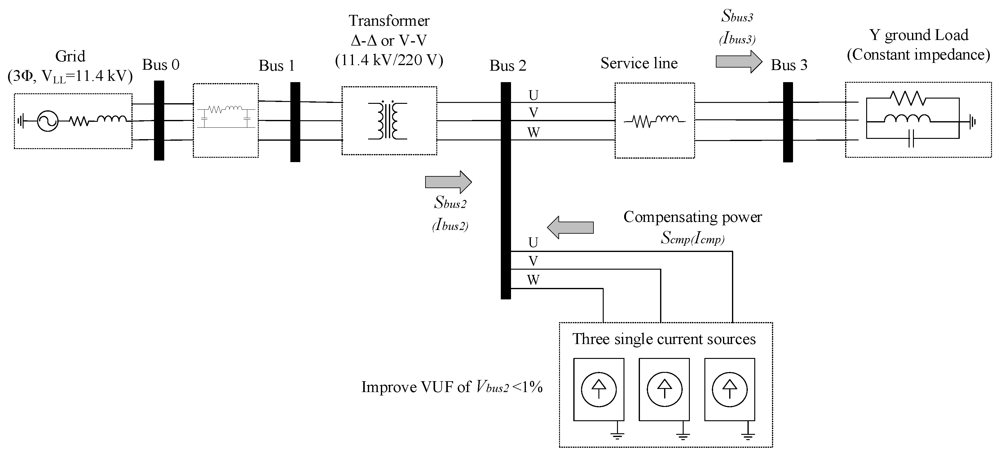
This study designed a simple three-bus distributed system to simulate the power flow of a three-phase unbalanced circuit, as shown in Figure 1. From left to right, the components are the equivalent grid, underground transmission line, transformer (connected by delta or open delta), service wires, and the equivalent impedance of lumped load. The proposed unbalance source, consisting of three single-phase current sources, is also shown.

The specific parameters of each part are described as follows. The equivalent grid was represented by a line-to-line voltage of 11.4 kV and a short capacity of 250 MVA, X/R ratio of 17.4, and it has four three-phase wires. The underground transmission line was represented by 500 MCM, a length of 10 km, an impedance of $0.2536+\mathrm{j}0.1464\Omega /\mathrm{km}$, and a rated current of 600 A, and it was simulated by the p model. Three-phase pole-mounted transformers were developed with two different structures. First, three single transformers were used to form a delta–delta connection. Second, two single transformers were used to form an open–delta to open–delta connection, which lacked the transformer of phase c. The single transformer was represented by $\frac{11.4}{\sqrt{3}}$ kV/220 V, impedances R₁ = R₂ = 0.365 (%, pu) and X₁ = X₂ = 1.58 (%, pu), R_m = 588.237 pu, and L_m = 162.075 pu. The service wires, connecting the transformer to the user meter, were represented by a resistance of 35 (Ω/m) and a length of 80 m. The maximum lumped load depended on the connection of the transformers. The loads were 500 kVA (167 kVA × 3) and 289.2 kVA (167 kVA × $\sqrt{3}$) for the delta–delta connection and the open–delta to open–delta connection, respectively. This study used Matlab/Simulink version 2020a to simulate the dynamic reaction during the unbalanced voltage improvement in the above circuits.

The user side was defined behind Bus 2, including the service wires and lumped load. The proposed compensation current source was connected to Bus 2. The injected three-phase currents were determined by the PSO algorithm to balance the voltage at Bus 2.

To simplify the study, only the situations of severe unbalance voltages were selected. These situations were among 60~100% of the total three-phase load, with a step change of 5%. The power factors were pure, 0.8 lagging, or 0.8 leading. As mentioned above, the rating capacity of the three-phase transformers were 500 kVA for the delta–delta connection and 289.2 kVA for the open–delta to open–delta connection. The voltage regulations at the load side were constrained with ±10% for the industrial user. In general, higher loads experienced higher unbalanced voltages.

The representative situations of severe unbalance factors were selected, and are shown in

Table 1. Loads of three single-phase currents for severe voltage unbalance cases.

Case	A	B	C
Structure	Transformer Δ–Δ connection supplies unbalance load	Transformer V–V connection supplies unbalance load	Transformer V–V connection supplies balance load
Power factor (pf)	1	1	0.8 lag
phase load (a, b, c) (%)	95, 65, 80	90, 70, 80	100, 100, 100
$\mathrm{VUF}{d}_0$ (%)	10.56	7.03	0
$\mathrm{VUF}{d}_2$ (%)	0.34	1.67	1.88

The power ratings of Cases A, B, and C were 167 kVA, 96.4 kVA, and 96.4 kVA, respectively.

. For the Δ–Δ connected transformer (Case A), the worst unbalanced voltages occurred at phase loads of 95%, 65%, and 80%, in phases a, b, and c, respectively. This resulted in VUFs of 10.56% and 0.34% in $d_0$ and $d_2$, respectively. On the contrary, both $d_2$% and $d_0$% were zero if the transformer supplied the balanced load. It is clear that the zero-sequence voltage is the most important factor.

The other two situations were the open–delta to open–delta connected transformers, supplying balanced loads (Case B) and unbalanced loads (Case C). For Case B, unbalanced voltages occurred at phase loads of 90%, 70%, and 80% in phases a, b, and c, respectively. This resulted in VUFs of 7.03% and 1.67% in $d_0$ and $d_2$, respectively. For Case C, unbalanced voltages occurred at three-phase balanced loads that resulted in VUFs of 0% and 1.88% in $d_0$ and $d_2$, respectively. Note that the voltage was unbalanced, even if the load was three-phase balanced. However, this situation is a common and difficult problem in practice.

4. Improvement of Unbalanced Voltage

The circuit analysis method was presented before using the algorithm method. Circuit analysis is a simple method that compensates each phase current by the difference between the phase current and the average current. The voltage of Bus 2, behind the transformer secondary side, could become balanced if the total current through Bus 2 was three-phase balanced. However, this method is only feasible for Δ–Δ and Y–Y connections, because the impedances of the transformer are balanced.

Equation (2) assumes the load is balanced, so that each phase load, $S_{bal}^{abc}$, became the average of three original single phases, $S_{bal}^{ave}$. The average load was the target of compensating each phase load. The compensating power of each phase was the original load minus the average load, as in Equation (3). Then, the command of the compensating power unit (VA) was transferred to the current unit (A) for the acceptable instruction of the device. The response was simulated by power flow analysis, where the voltage of Bus 2 was solved and was equal to the voltage of the compensation device, $V_{bal}^{abc}$. Then, the compensating current was found by dividing by the voltage, as in Equation (4).

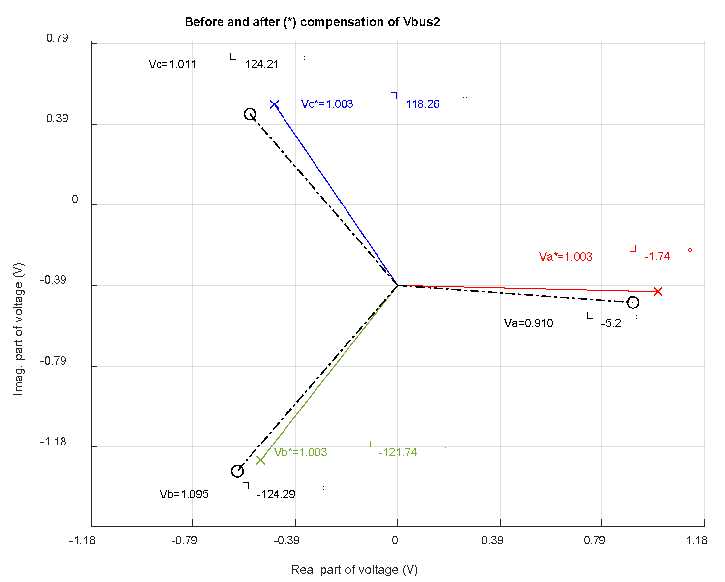
For Case A in Table 1, the Δ–Δ connection supplying unbalanced loads, the phase voltages Va, Vb, and Vc were 0.910 $\angle$ −5.2° pu, 1.095 $\angle$ −124.29° pu, and 1.011 $\angle$ 124.21° pu, respectively. These magnitudes of voltage are proportional to the load conditions. The lowest voltage, Va, was in phase a, with the highest load, 90%. The highest voltage, Vb, was in phase b, with the lowest load, 65%. Larger loads had lower voltaged because the voltage dropped on the impedance of lines.

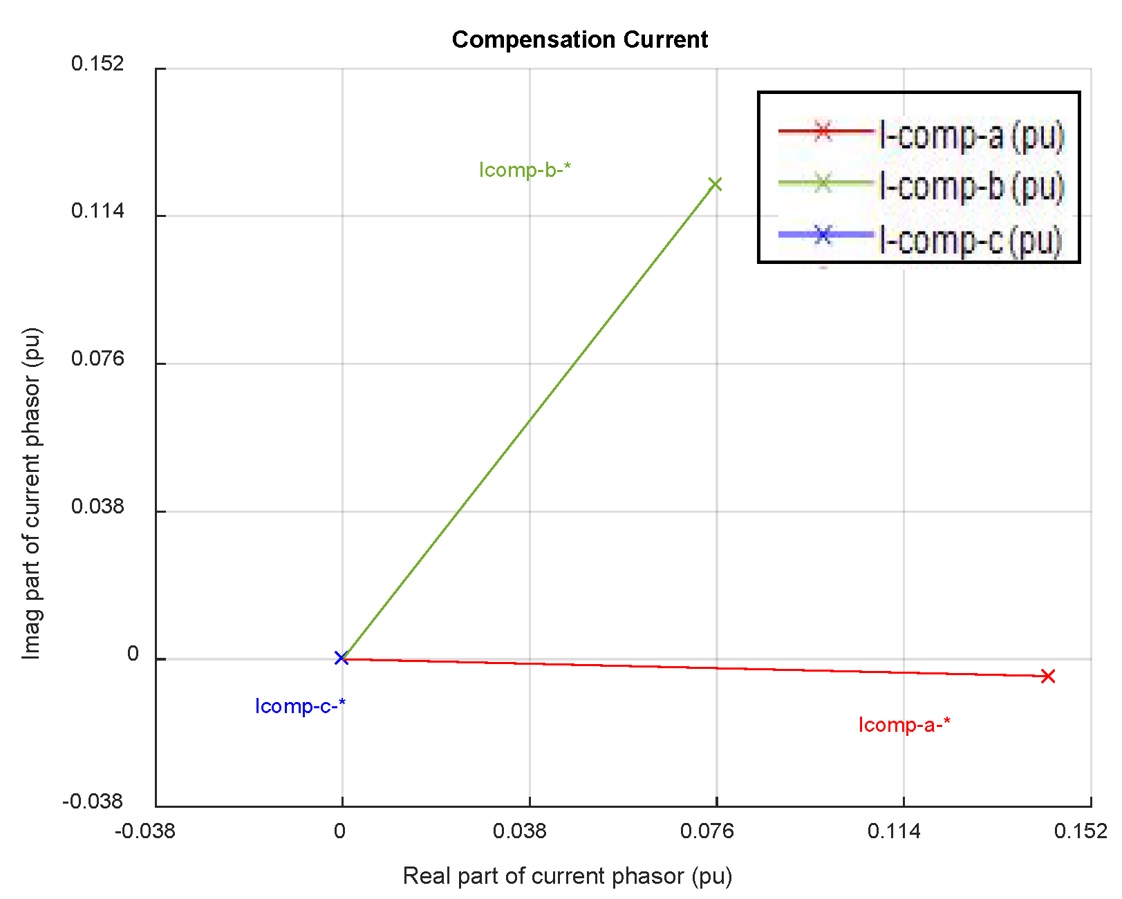
According to Equations (2)–(4), the compensation current, $I_{comp}^{abc}$, was calculated as $0.144\angle -1.74°$ pu, $0.144\angle 58.26°$ pu, and $0.0004\angle 118.24°$ pu, where the current base was 1312.2 A. These compensated currents are shown in Figure 2 through the current phasor diagram. These currents are also related to the load conditions, where a higher load received a higher compensation current in the phase line at Bus 2. The currents A and B were higher because their loads were higher than average load. The load C was equal to the average load, such that current C was almost zero. Note that the compensation currents were in a negative sequence.

$$S_{bal}^{ave}=\frac{S_{load}^a+S_{load}^b+S_{load}^c}{3}$$

(2)

$$\{\begin{array}{c}{S}_{comp}^a=S_{load}^a-S_{bal}^{ave}\\ S_{comp}^b=S_{load}^b-S_{bal}^{ave}\\ S_{comp}^c=S_{load}^c-S_{bal}^{ave}\end{array}$$

(3)

$$\{\begin{array}{c}{I}_{comp}^a={\left(\frac{S_{comp}^a}{V_{bal}^a}\right)}^{*}\\ I_{comp}^b={\left(\frac{S_{comp}^b}{V_{bal}^b}\right)}^{*}\\ I_{comp}^c={\left(\frac{S_{comp}^c}{V_{bal}^c}\right)}^{*}\end{array}$$

(4)

After compensating, the currents of the secondary side of the transformer were balanced. The voltages at the secondary side of the transformer became balanced because of the balanced transformer structure and balanced currents. The phasors of the original and compensated voltages are compared in Figure 3. The compensated voltages were 1.003$\angle$ −1.74° V, 1.003$\angle$ −121.74° V, and 1.003$\angle$ 118.26° V, which are shown in red, green, and blue color, respectively. The VUF was improved from 10.56% to 0%. Each phase voltage was 1.003, which is similar to a nominal voltage 1.0 pu, and each phase was shifted by 120°.

Table 2. Power flow with compensation by the circuit analysis method in Case A.

	Power at Secondary Side of Transformer (pu)	Power at Compensator (pu)	Power at Load (pu)
Phase a	$0.262\angle$ 0.0°	$0.048\angle$ 0.00°	$0.310\angle$ 0°
Phase b	$0.262\angle$ 0.0°	$0.048\angle$ −180°	$0.214\angle$ 0°
Phase c	$0.262\angle$ 0.0°	$0.000\angle$ 0.00°	$0.262\angle$ 0°
Three-phase power	$0.787\angle$ 0°	0	$0.787\angle$ 0°

Sbase was 500 kVA.

shows the apparent power at the transformer, compensator, and load after compensation. The apparent three-phase power was approximately equal to 0.262 pu. The loads of phases a, b, and c were 0.310, 0214, and 0.262, respectively, equal to 95%, 65%, and 80% of rating power with the same setting value. The compensating power of phases a and b were 0.048$\angle$0° and 0.048$\angle$−180°, respectively, with the same magnitude but opposite phasor angles. Note that the total apparent power of the compensator was approximately zero for the constraint setting. The zero power represents that no energy was dissipated and developed in the compensator.

Although the circuit analysis method provided solutions for a balanced transformer with unbalanced load, it could not solve the unbalanced connection of transformers in this study. As the assumption was that the measurement of voltage and current were at the secondary side, the effect of the unbalanced impedance of the transformer was not accounted for. Even if balanced currents are easily achieved, the unbalanced impedance of the transformer may cause unbalanced voltages. In addition, the parameters of the whole circuit should be known while using the circuit analysis method. However, the parameters are not available in practice. Hence, this study proposed a PSO algorithm to solve the compensation current.

5. Compensation Based on PSO Algorithm

5.1. Setting of the PSO Algorithm

In contrast to the circuit analysis method, the optimal algorithm reaches the optimal solution according to the feedback from the previous response of the circuit network. Compared with PID control, the benefits of this method are not reliant upon the parameters of whole circuit devices.

There are many popular optimal algorithms for nonlinear problems, such as particle swarm optimization (PSO) [15], moth–flame optimization (MFO) [16], ant colony optimization (ACO) [17], and genetic algorithms (GA) [18]. The selection of an optimal algorithm could be an avenue for further study because this study focuses on the improvement of unbalanced voltages. The comparison of different optimal algorithms was not considered in this study. This study used PSO due to the advantages of a fast searching duration, higher dimensional variables, and acceptance of a nonoptimal solution [19,20,21].

The fitness function of PSO, shown in Equation (5), is related to Equation (1) because it is more suitable in a grounding system. To accelerate the speed of searching, each term of Equation (1), $d_0$ and $d_2$, are quadratic.

$$fitness={(d_{0,\mathrm{bus}2})}^2+100{(d_{2,\mathrm{bus}2})}^2$$

(5)

where $d_{0,\mathrm{bus}2}$ and $d_{2,\mathrm{bus}2}$ are the unbalanced factors of the zero sequence and negative sequence of Bus 2, respectively.

In total, six controllable variables were used to represent three magnitudes and three phase angles of three-phase compensation current phasors. The controllable variables were $\left|I_{comp}^0\right|$, $\left|I_{comp}^1\right|$, $\left|I_{comp}^2\right|$, ${\theta }_{comp}^0$, ${\theta }_{comp}^1$, and ${\theta }_{comp}^2$ in compensation currents. The constraints were current limits, reasonable phase angles, and three-phase apparent powers, as in Equations (6)–(8). In Equation (6), the current limits, 200 A, were approximately 15% of the rated load. The maximum power of the single-phase compensator was 165 kVA.

$$\{\begin{array}{c}0\le \left|I_{comp}^0\right|\le 200\\ 0\le \left|I_{comp}^1\right|\le 200\\ 0\le \left|I_{comp}^2\right|\le 200\end{array}$$

(6)

where $\left|I_{comp}^0\right|,\left|I_{comp}^1\right|$, $\mathrm{and}\left|I_{comp}^2\right|$ are the magnitudes of compensation currents, (A).

In Equation (7), the reasonable angles were set to prevent wasting time searching with a large angle shift. The angles of the compensation current were negative-sequence because of the unbalanced current. The possible range of symmetric phases was (−120°)~(120°).

$$\{\begin{array}{c}-120°\le {\theta }_{comp}^0\le 120°\\ -120°\le {\theta }_{comp}^1\le 120°\\ -120°\le {\theta }_{comp}^2\le 120°\end{array}$$

(7)

where ${\theta }_{comp}^a$, ${\theta }_{comp}^b$, and ${\theta }_{comp}^c$ are the angles of compensation currents, (degree).

In Equation (8), the net three-phase apparent powers were restricted to zero, such that the power was not developed and dissipated in the compensator.

$$\sum \left|S_{comp}^a+S_{comp}^b+S_{comp}^c\right|=0$$

(8)

where $S_{comp}^a$, $S_{comp}^b$, $\mathrm{and}{S}_{comp}^c$ are the compensating apparent power (VA).

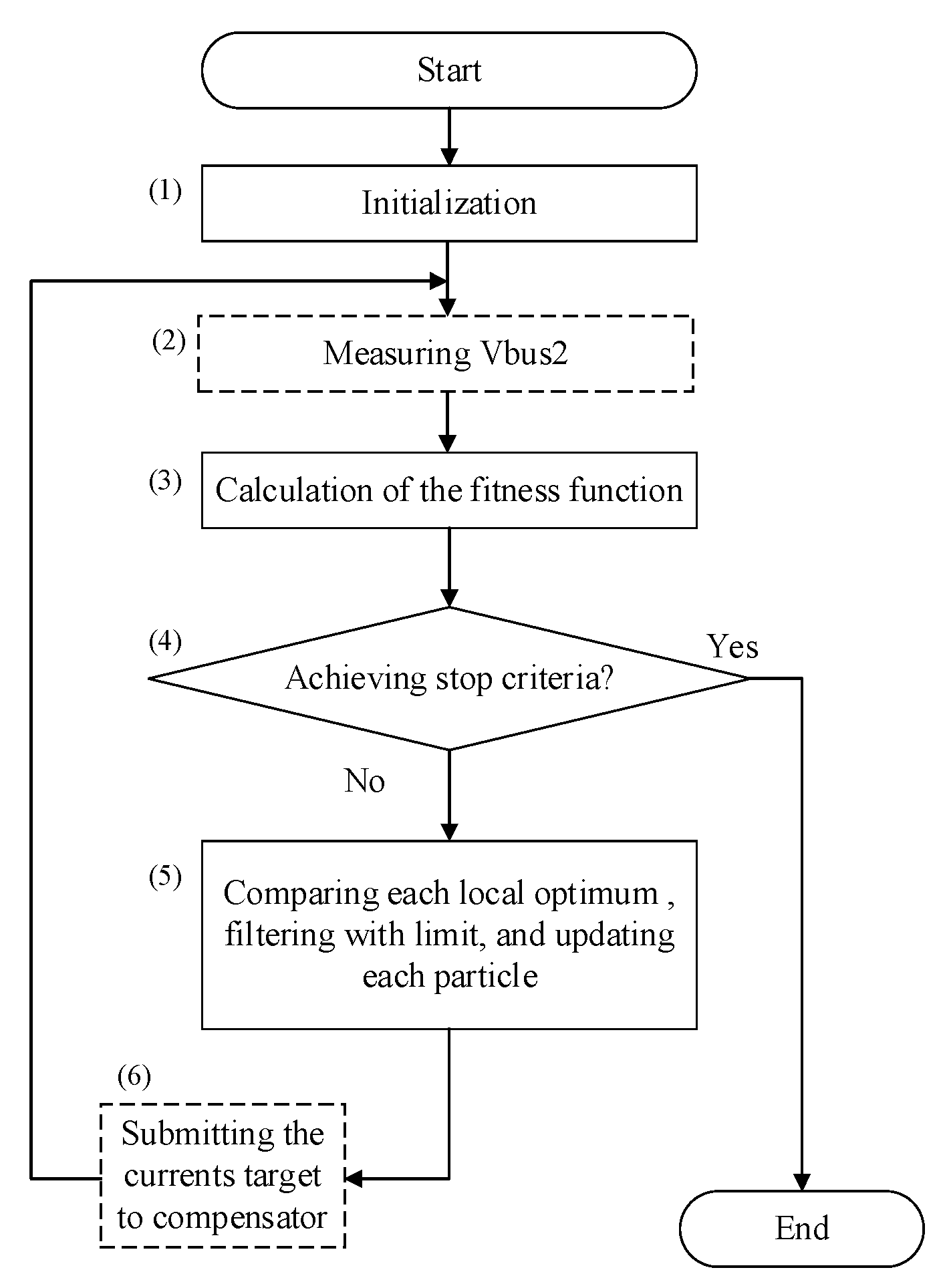
Figure 4 shows a flow chart of the PSO process utilized in this study. Each step was introduced as follows. The blocks drawn by dashed lines are related to the power grid.

• Step 1: Initialize the variables in PSO, such as setting the number of particles at 20. Each particle was in six-dimensional space, denoted as $x_i^t=\left[x_{i1}^t,x_{i1}^t,\dots ,x_{iD}^t\right]$. The velocity of the particle was denoted as $v_i^t=\left[v_{i1}^t,v_{i1}^t,\dots ,v_{iD}^t\right]$. The iteration times, $t$, were limited to $MaxItr$, 20.
• Step 2: Measure the current voltages of Bus 2 for calculating the VUF. Note that the voltage could change after the response of the compensator reacted in Step 6.
• Step 3: Calculate the fitness function of each particle at the current state, as in Equation (5).
• Step 4: Check the stopping criteria:
  Target requirement satisfied that VUF is lower than 1%.
  Target requirement not satisfied but iteration times $t>MaxItr$.
• Step 5: If the local optimum was less than the global optimum, the global optimum was replaced by the local optimum to maintain the current state. Then, the learning factors ($c_{1}and{c}_2)$ and inertia coefficient ($w$) were updated, and the powers of $\alpha ,\beta$, and $\gamma$ were used to accelerate the convergence rate and increase accuracy, as expressed in Equations (9)–(11). Each particle was updated as in Equations (12)–(13) to generate new optimums.
  If the optimums did not satisfy Equation (8), then the modification was conducted by Equation (14).
• Step 6: Submit the new current target, as solved using PSO, to the compensator.

Figure 4. Flow chart of PSO.

Figure 4. Flow chart of PSO.

$$w=w_{min}+{\left(\frac{\left(MaxItr-t\right)}{MaxItr}\right)}^{\alpha }\left(w_{max}-w_{min}\right)$$

(9)

$$c_1=c_1{}_{min}+{\left(\frac{\left(MaxItr-t\right)}{MaxItr}\right)}^{\beta }\left(c_1{}_{max}-c_1{}_{min}\right)$$

(10)

$$c_2=c_2{}_{max}+{\left(\frac{\left(MaxItr-t\right)}{MaxItr}\right)}^{\gamma }\left(c_2{}_{min}-c_2{}_{max}\right)$$

(11)

where the inertia coefficient,$w$, had a default setting of 0.2; $w_{max}$ and $w_{min}$ are the boundaries of $w$, with defaults of −0.8 and 0.2. Learning factors, $c_1$ and $c_2$, had defaults of 2.5 and 0.5. The maximum and minimum, $c_{max}$ and $c_{min},$ were 2.5 and 0.5; $\alpha$, $\beta$, $\mathrm{and}\gamma$ are the powers of $w$, $c_1$, and $c_2$, set at 1.2, 1.5, and 2, respectively.

$$x_i^{t+1}=x_i^t+v_i^{t+1}$$

(12)

$$v_i^{t+1}=w{v}_i^t+c_1{R}_1\left(x_{i,PB}^t-x_i^t\right)+c_2{R}_2\left(x_{i,GB}^t-x_i^t\right)$$

(13)

where $x_{PB}^t$ was the best in one particle, and $x_{GB}^t$ was the best in whole particles.

$$\{\begin{array}{c}ave=\frac{V_2^a{x}_i^a+V_2^b{x}_i^b+V_2^c{x}_i^c)}{3}\\ x_i^a={\left(\frac{V_2^a{x}_i^a-\mathrm{ave}}{V_2^a}\right)}^{*}\\ x_i^b={\left(\frac{V_2^b{x}_i^b-\mathrm{ave}}{V_2^b}\right)}^{*}\\ x_i^c={\left(\frac{V_2^c{x}_i^c-\mathrm{ave}}{V_2^c}\right)}^{*}\end{array}$$

(14)

5.2. Simulation Results

The situations of Case B and Case C in Table 1 are discussed. These cases can simply demonstrate the effect of compensation.

(1)

Case A: delta–delta connection supplying unbalanced loads

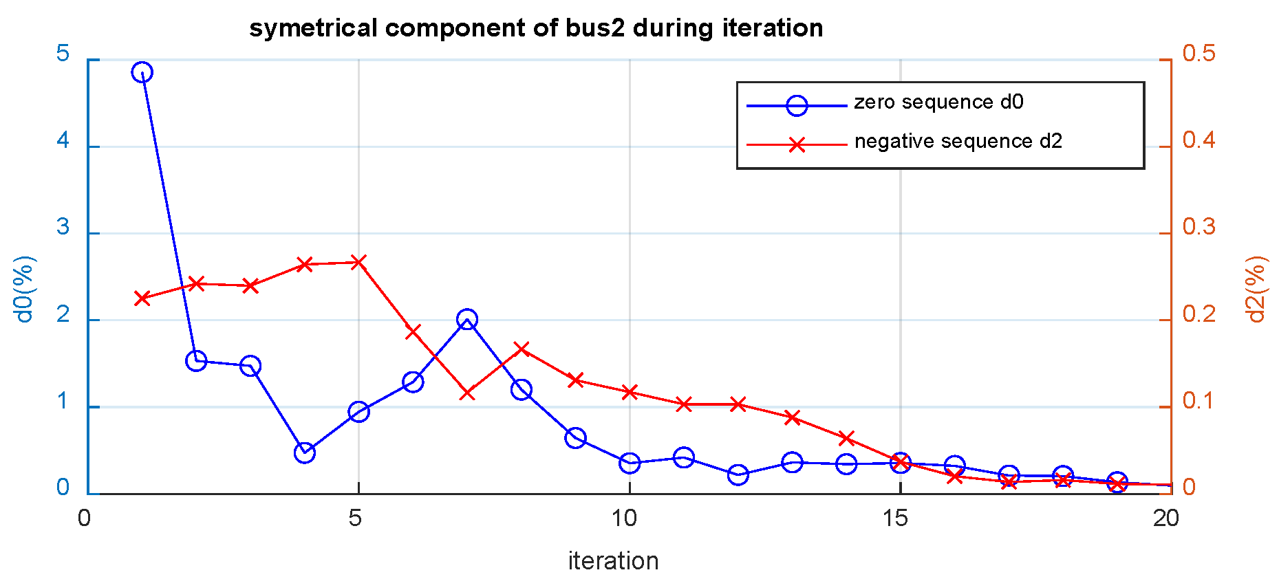
Figure 5 shows the zero-sequence $d_0\%$ and negative-sequence $d_2\%$ in each iteration from the PSO algorithm. The scale of the right vertical axis is ten times that of the left vertical axis. The $d_0\%$ decreased promptly in the beginning and then followed a peak of fluctuations before finally decreasing gradually. The trend of $d_2\%$ was the opposite of $d_0\%$ in early iterations, before decreasing gradually in later iterations. A total of 13 iterations were required to achieve $d_0\%$ and $d_2\%$ values that were both lower than 1.0%. Furthermore, the minimum values were 0.01% and 0.10% for $d_0\%$ and $d_2\%,$ respectively, at the end of the simulation. The evolution of the zero sequence and negative sequence showed that they experience opposite changes in the short term and similar changes in the long term.

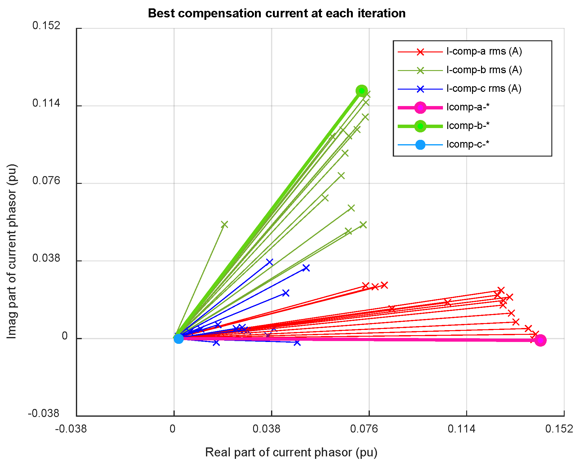
Figure 6 shows the best compensation current phasors in 20 iterations. The phasors with marker circles are the best values of all iterations; for phases a, b, and c, these were $0.143\angle -0.37°$ pu, $0.142\angle 58.9°$ pu, and $0.002\angle -5.0°$ pu, respectively, where the current base was 1312.2 A. The best solution is approximately the same as that shown in Figure 2, solved by the circuit analysis method. The phasors with marker crosses show the searching process and the trend from the initial solution to the best solution. The searching ability of PSO was proved through many successful results which began from different initial solutions.

Table 3. Voltage unbalanced factor and voltage variation in Case A.

		$\mathbf{W}/\mathbf{O}\mathbf{Compensation}\left(\mathit{i}\right)$	$\mathbf{With}\mathbf{Compensation}\left(\mathit{j}\right)$	Change $\mathbf{k}=\left|\mathit{j}\right|-\left|\mathit{i}\right|$
$\mathrm{bus}2\_d_0$(%)		10.56	0.10	−10.46
$\mathrm{bus}2\_d_2$(%)		0.34	0.01	−0.33
Voltage	Phase a	0.910 ∠ −5.2°	1.002 ∠ −1.7°	0.092
	Phase b	1.095 ∠ −124.3°	1.002 ∠ −121.8°	−0.093
	Phase c	1.011 ∠ 124.2°	1.003 ∠ 118.3°	−0.007
Variation (%)	Phase a	−9.00	0.18	−8.82
	Phase b	9.51	0.19	−9.32
	Phase c	1.05	0.34	−0.71

shows the comparison with and without compensations. The $d_0\%$ of Bus 2 greatly decreased from 10.56% to 0.10%, with an improvement of 10.46%. The $d_2\%$ of Bus 2 slightly decreased from 0.34% to 0.01%, with an improvement of 0.33%. The improved $d_0\%$ was slightly higher than the improved $d_2\%$, although they were both less than 1%. This reveals that the zero-sequence voltage is the major problem, even in the approximate balancing load.

For a–b–c phase analysis, the voltage phasors without compensation were unbalanced. The voltage of phase a, 0.910 pu, was much smaller because of the heavy load. In contrast, the voltage of phase b, 1.095 pu, was higher because of the lighter load. The voltage of phase c, 1.011 pu, was closest to the nominal value.

In the case with compensation, it is clear that the magnitudes of phasors Va, Vb, and Vc were corrected to 1.002, 1.002, and 1.003 pu. Thus, the magnitude of each phase became very similar. The magnitudes of phases a and b saw the greatest changes. In addition, the difference of phase angles between nearby phasors became approximately 120°. The phase shift was approximately −1.9°.

It is an ancillary benefit that voltage variations of each phase were reduced to less than 0.34%. Note that without compensation, the voltage variations of phase a, with the heaviest load, and phase b, with the lightest load, were –9.00% and +9.51%, respectively, almost opposite, with a change of ±10%. Thus, the tap changer of the transformer cannot significantly improve the voltage variations because either increasing or decreasing the position of the tap causes the opposite criterion in each side.

Table 4. Apparent power at transformer, compensator, and load in Case A.

	Power at Secondary of Transformer (pu)	Power at Compensator (pu)	Power at Load (pu)
Phase a	0.262 ∠ 0°	0.048 ∠ −1.3°	0.310 ∠ 0°
Phase b	0.261 ∠ 0°	0.048 ∠ 179.3°	0.214 ∠ 0°
Phase c	0.263 ∠ 0°	0.001 ∠ 123.3°	0.263 ∠ 0°
Three phase	0.787 ∠ 0°	0 ∠ 0°	0.787 ∠ 0°

Sbase was 500 kVA.

shows the power flow at the secondary of the transformer, compensator, and load. The three single-phase powers of the transformer secondary were approximately the ideal target, $0.267\angle$0° pu. The phase loads were 0.310 pu, 0.214 pu, and 0.263 pu, equal to the ratio of each phase and a single rating by 93.0%, 64.2%, and 78.9%, respectively. Note that the sum of the three-phase compensation power was approximately zero, obeying the constraints in the algorithm. The compensation power of phase a, 0.048 ∠ −1.3° pu, included a higher real power that was supplied to decrease the load in phase a. The compensation power of phase b, 0.048 ∠ 179.3° pu, included a higher negative real power to increase the load in phase b. The compensation power of phase c, 0.001 ∠ 123.3° pu, included a higher reactive power to act against the compensation reactive power of phases a and b.

(2)

Case B: open–delta to open–delta connection supplying unbalanced loads

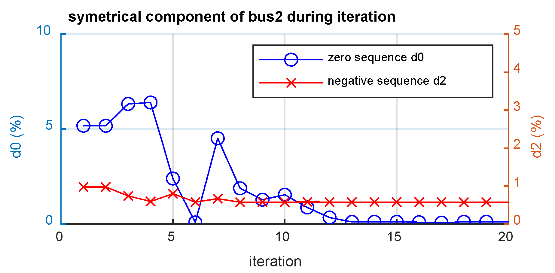
In Case B, the open–delta to open–delta connection lacked a transformer of phase c, hence, the circuit analysis method was probably not feasible. Figure 7 shows that the PSO algorithm took six iterations and decreased abruptly to less than 1.0%, and the minimum value was 0.84% at the 12th iteration.

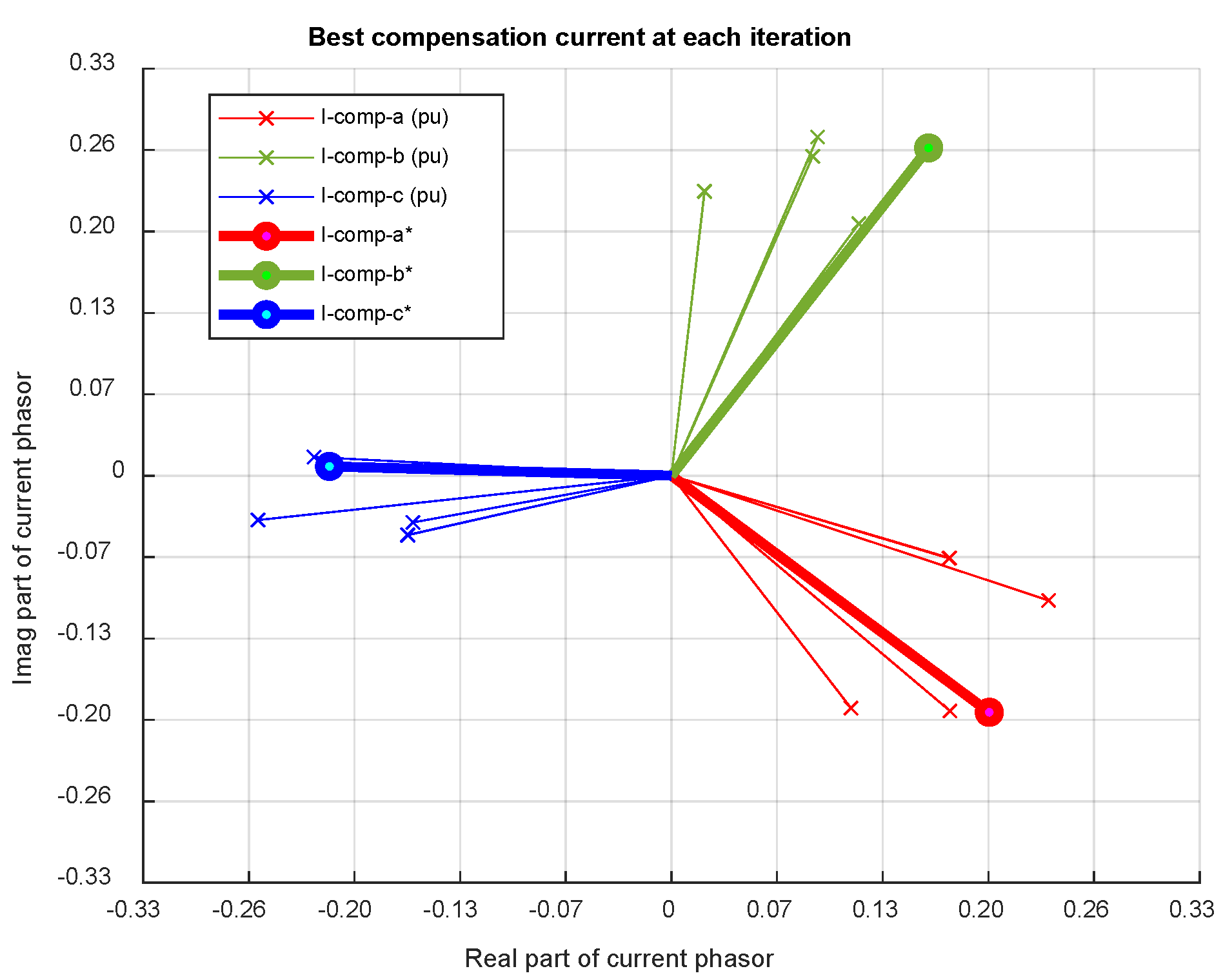
Figure 8 shows the best compensation current of each iteration. The phasors with marker circles were the best values of all iterations; for phases a, b, and c, these were $0.276\angle -44.0°$ pu, $0.311\angle 58.8°$ pu, and 0.214$\angle 178.0°$ pu, respectively, where the current base was 757.6 A. The current of phase b was larger than other phases, even though the load of phase b was the smallest. The reason is the lack of a transformer connecting to phases a and c, thus, the current of phase b was equal to the sum of currents in phases a and c. The compensation of phases a and c were higher because of the heavier loads, 90% and 80%, respectively. However, the compensation of phase c was smaller because of the smaller load, 70%.

Table 5. Voltage unbalanced factor and voltage variation in Case B.

		$\mathbf{W}/\mathbf{O}\mathbf{Compensation}\left(\mathit{i}\right)$	$\mathbf{With}\mathbf{Compensation}\left(\mathit{j}\right)$	Change $\mathbf{k}=\left|\mathit{j}\right|-\left|\mathit{i}\right|$
$\mathrm{bus}2\_d_0$(%)		7.03	0.11	−6.92
$\mathrm{bus}2\_d_2$(%)		1.67	0.58	−1.09
Voltage	Phase a	0.927 ∠ −4.4°	0.997 ∠ −1.7°	0.070
	Phase b	1.068 ∠ −122.9°	1.005 ∠ −121.3°	−0.063
	Phase c	1.016 ∠ 121.5°	1.009 ∠ 118.2°	−0.007
Variation (%)	Phase a	−7.28	−0.28	−7.00
	Phase b	6.79	0.53	−6.24
	Phase c	1.64	0.87	−0.75

shows the comparison with and without compensations. The $d_0\%$ of Bus 2 greatly decreased from 7.03% to 0.26%, which improved by 6.77%. The $d_2\%$ of Bus 2 slightly decreased from 1.67% to 0.88%. Note that, in contrast to Case A, the $d_2\%$ was slightly higher than $d_0\%$. This reveals that the negative-sequence voltage is the major problem in the unbalanced connection of a transformer.

The voltage variations of phase a, with the heaviest load, and phase b, with the lightest load, were –7.28% and +6.79%, respectively, almost opposite, with a change of ±10%. Thus, the tap changer of the transformer cannot significantly improve the voltage variations.

In

Table 6. Apparent power at transformer, compensator, and load in Case B.

	Power at Secondary of Transformer (pu)	Power at Compensator (pu)	Power at Load (pu)
Phase a	0.235 ∠ −15.3°	0.092 ∠ 42.3°	0.294 ∠ 0°
Phase b	0.338 ∠ −0.1°	0.104 ∠ 179.8°	0.234 ∠ 0°
Phase c	0.240 ∠ 15.0°	0.072 ∠ −59.8°	0.268 ∠ 0°
Three phase	0.796 ∠ 0.0°	0 ∠ 0°	0.796 ∠ 0°

Sbase was 289.3 kVA.

, the power supplied into the phase loads were 0.294 pu, 0.234 pu, and 0.268 pu, equal to the ratio of each phase and a single rating by 88.2%, 70.2%, and 80.4%, respectively. The sum compensation power of phase a, 0.092 $\angle$ 42.3° pu, consisted of a real power to supply energy. In contrast, the compensation power of phase b, 0.104 $\angle$ 179.8° kVA, consisted of a negative real power to absorb energy. The sum of the three-phase compensation power was approximately 0 VA, which obeys the constraints of the algorithm.

Although the voltage of the secondary of the transformer was approximately balanced, the power of the transformer was unbalanced. The phase b of the transformer supplied the highest power, 0.338 pu, which was approximately 93.2% of the single-phase rating. The overcurrent of the cable should be improved in the open–delta connection transformer.

(3)

Case C: open–delta to open–delta connection supplying balanced loads

The performance of the algorithm was verified above. Hence, the study of Case C focused on the variation of load, including low, medium, and high degrees.

Constant power factor, 0.8 lagging, of balanced load connected to open–delta transformer

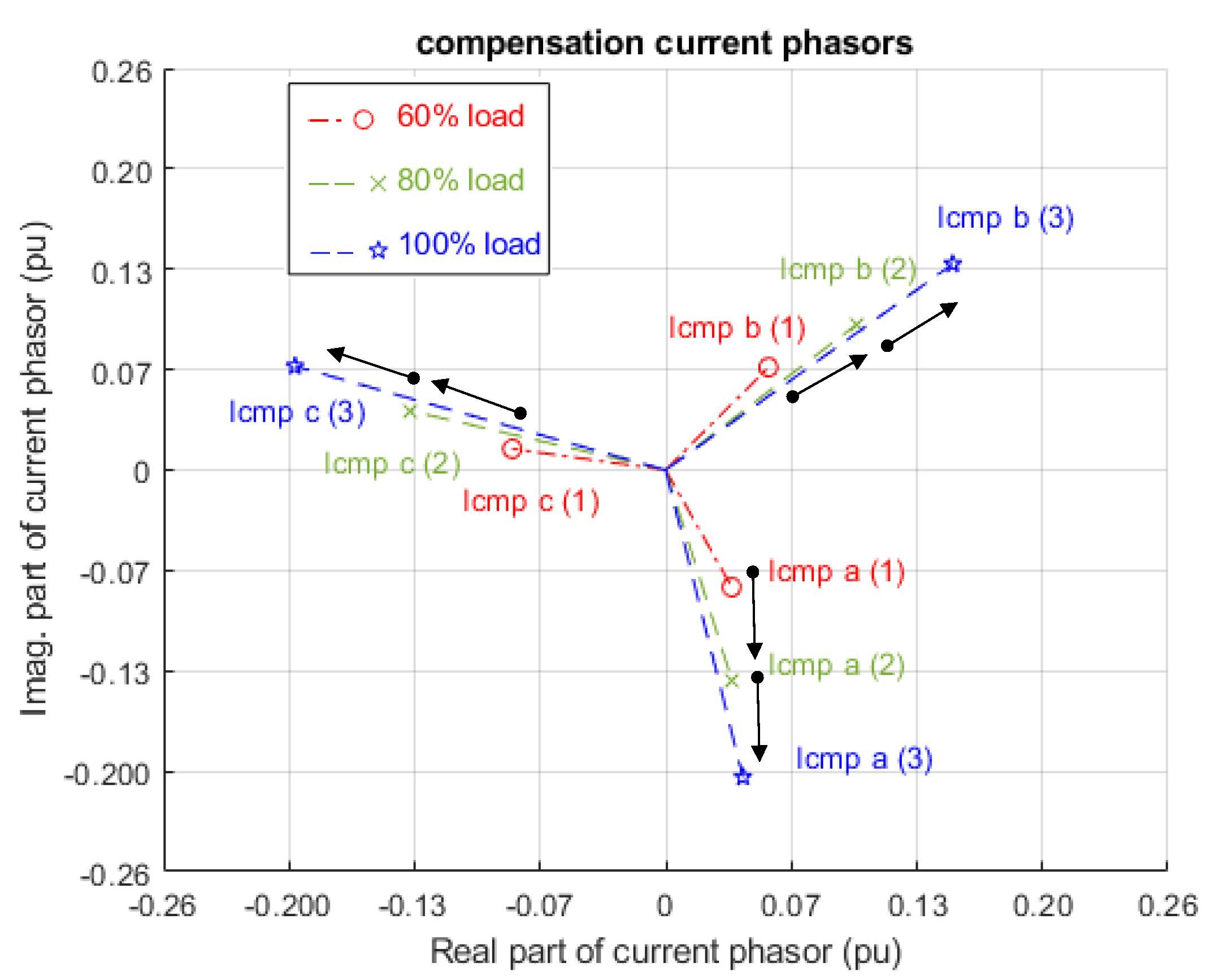
Figure 9 shows the relationship of compensation currents with increasing inductive loads, where the total loads of three phase were set at 60%, 80%, and 100%. Note that the unbalance factor was lower than 1% when the total load was lower than 60%; thus, they were not considered. The unbalanced factor in each load could be corrected to less than 1.0%. It was found that the phasors of compensation currents expectedly increased while increasing the total load. The magnitude of compensation currents increased, but the angle of compensation currents remained similar. This relationship might be useful to predict the compensation current when the load is changing.

Constant power factor, 0.8 leading, of balanced load connected to open–delta transformer

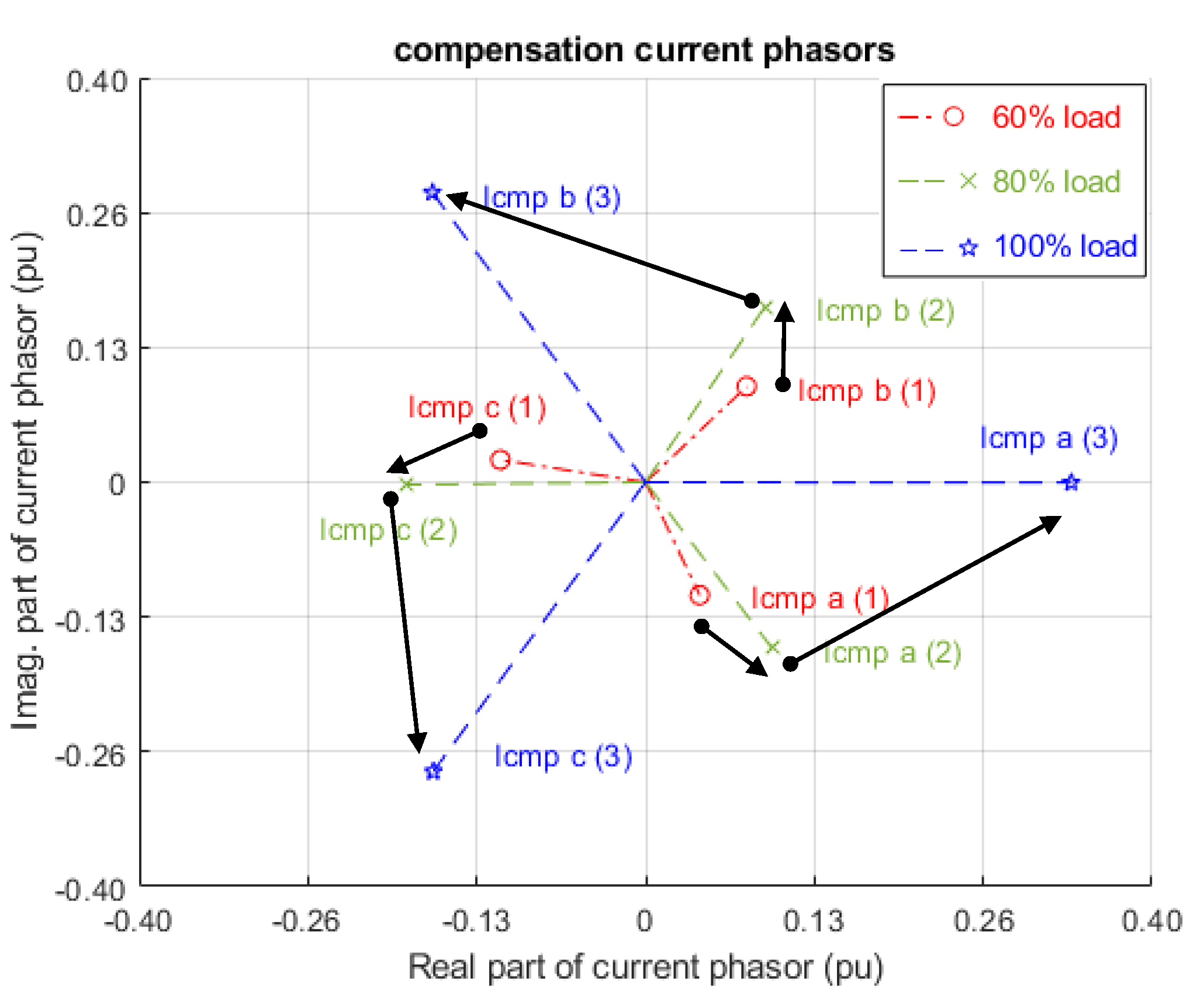
Figure 10 shows the relationship of compensation currents with increasing capacitive loads, where the total loads of three phase were set at 60%, 80%, and 100%. The magnitude of compensation currents increased from 0.12 pu to 0.33 pu. In contrast to the inductive load with a consistent angle, the angle of phasors decreased with increasing load. Thus, the phasors rotated counterclockwise when the load increased.

6. Discussion

In practice, the main target of improvement is that the $d_0\%$ and $d_2\%$ of VUF should both be less than 1%, which is within the regulation. Otherwise, the higher power and cost of devices would be overinvested for minimal improvement.

For real applications, the values of particles in each iteration are the command of the power compensator. After responses are finished, the measured voltages are used to calculate the unbalanced factor as the feedback. The reaction of the proposed method is feasible if the searching optimal solution is shorter than the variations of load, which are usually in the order of minutes.

The number of iterations of the searching optimal solution is affected by the setting of the maximum iterations, according to Equations (10)–(12) and the number of particles. The relationship of maximum iterations and particles in Case B (open–delta connections), for a statistically iterated number, are shown in

Table 7. Effect of expended iterations related to maximum iterations and particle number.

Mean/ Standard	Particle Number
	10		20	40	80
Max Iterations	10	NaN	5.6/2.3 *	6.7/1.6	5.5/1.6
	20	14.6/4.3 *	11.7/2.2	8.6/1.8	7.0/1.7
	40	12.6/2.9	13.6/4.4	9.7/2.8	6.41/9
	80	16.5/5.5	15.2/4.2	10.8/2.0	7.3/2.4

. The mean and standard deviation were calculated from the results of 10 simulations. For example, the average iterated number was 7.3 and the standard deviation was 2.4, with the PSO setting of 80 particles and 80 maximum iterations. Whole tests were failed if the settings of particles and maximum iterations were both 10. There were few failures in cases of lower particle and maximum iteration settings, marked with “*”.

It was found that the higher the maximum iterations, the more iterations, and the higher the particle number, the fewer iterations. Additionally, the higher the maximum iterations, the lower the particle number required. The suggested settings in this study were 20~40 for maximum iterations and 10~40 for the particle number.

Additionally, the maximum current of the compensator was approximately 0.25 pu in Case B. Hence, the capacity of the compensator was suggested to be approximately 25% of the load. The performance of the compensation is worse with a lower power of the compensator.

The unbalance voltage factor is influenced by the connection of the transformer and the magnitude of each phase load. As well as the delta–delta and open–delta to open–delta connections, the open–delta to open–Y connection, known as a U–V connection, is widely used in distributed networks. The proposed method could also be feasible for this connection.

7. Conclusions

A three-phase voltage balancing method using a PSO controller was presented in this paper. This method can improve the unbalanced factors ($d_0$ and $d_2$) to both be less than 1% in the delta–delta transformer and the open–delta to open–delta transformer. Meanwhile, the net compensation power of three phases can be almost zero, so that no energy is released or dissipated inside the compensator.

The proposed method was checked for similar performance to the analysis method. However, this method does not require the circuit parameters as the analysis method does, thus, it is feasible to be used in practice. Note that the PSO can be replaced by other optimal algorithms because this paper focused on the improvement of unbalanced voltages.

In further research, other connections of transformers can be verified. In addition, the three-phase voltage balancing function presented in this paper can be included in an energy storage system (ESS). This type of ESS has a small capacity that can be installed in the distribution grid. The aggregation of such a large number of ESSs is an avenue for further study.

References

- Chen, T.-H.; Yang, C.-H.; Yang, N.-C. Examination of the definitions of voltage unbalance. Int. J. Electr. Power Energy Syst. 2013, 49, 380–385. [Google Scholar] [CrossRef]
- Liao, R.-N.; Yang, N.-C. Evaluation of voltage imbalance on low-voltage distribution networks considering delta-connected distribution transformers with a symmetrical NGS. IET Gener. Transm. Distrib. 2018, 12, 1644–1654. [Google Scholar] [CrossRef]
- Lee, Y.-D.; Jiang, J.-L.; Ho, Y.-H.; Lin, W.-C.; Chih, H.-C.; Huang, W.-T. Neutral Current Reduction in Three-Phase Four-Wire Distribution Feeders by Optimal Phase Arrangement Based on a Full-Scale Net Load Model Derived from the FTU Data. Energies 2020, 13, 1844. [Google Scholar] [CrossRef]
- Tan, Y.; Wang, Z. Incorporating Unbalanced Operation Constraints of Three-Phase Distributed Generation. IEEE Trans. Power Syst. 2019, 34, 2449–2452. [Google Scholar] [CrossRef]
- Liu, Y.; Li, J.; Wu, L. Coordinated Optimal Network Reconfiguration and Voltage Regulator/DER Control for Unbalanced Distribution Systems. IEEE Trans. Smart Grid 2019, 10, 2912–2922. [Google Scholar] [CrossRef]
- Singh, B.; Solanki, J. A Comparison of Control Algorithms for DSTATCOM. IEEE Trans. Ind. Electron. 2009, 56, 2738–2745. [Google Scholar] [CrossRef]
- Salmeron, P.; Litrán, S.P. Improvement of the Electric Power Quality Using Series Active and Shunt Passive Filters. IEEE Trans. Power Deliv. 2010, 25, 1058–1067. [Google Scholar] [CrossRef]
- Wang, D.; Mao, C.; Lu, J.; He, J.; Liu, H. Auto-balancing transformer based on power electronics. Electr. Power Syst. Res. 2010, 80, 28–36. [Google Scholar] [CrossRef]
- Yan, S.; Tan, S.-C.; Lee, C.-K.; Ron Hui, S.Y. Reducing Three-Phase Power Imbalance with Electric Springs. In Proceedings of the 5th International Symposium on Power Electronics for Distributed Generation Systems (PEDG), Galway, Ireland, 24–27 June 2014; IEEE Publications: New York, NY, USA, 2014. [Google Scholar]
- Li, P.; Ji, H.; Wang, C.; Zhao, J.; Song, G.; Ding, F.; Wu, J. Optimal Operation of Soft Open Points in Active Distribution Networks Under Three-Phase Unbalanced Conditions. IEEE Trans. Smart Grid 2019, 10, 380–391. [Google Scholar] [CrossRef]
- Sun, F.; Ma, J.; Yu, M.; Wei, W. Optimized Two-Time Scale Robust Dispatching Method for the Multi-Terminal Soft Open Point in Unbalanced Active Distribution Networks. IEEE Trans. Sustain. Energy 2021, 12, 587–598. [Google Scholar] [CrossRef]
- Wang, J.; Zhou, N.; Chung, C.Y.; Wang, Q. Coordinated Planning of Converter-Based DG Units and Soft Open Points Incorporating Active Management in Unbalanced Distribution Networks. IEEE Trans. Sustain. Energy 2020, 11, 2015–2027. [Google Scholar] [CrossRef]
- Guo, P.; Xu, Q.; Yue, Y.; Ma, F.; He, Z.; Luo, A.; Guerrero, J.M. Analysis and Control of Modular Multilevel Converter With Split Energy Storage for Railway Traction Power Conditioner. IEEE Trans. Power Electron. 2020, 35, 1239–1255. [Google Scholar] [CrossRef]
- Cooper, C.B. IEEE Recommended Practice for Electric Power Distribution for Industrial Plants. IEEE Stand. 1993, 141, 658. [Google Scholar]
- Del Valle, Y.; Venayagamoorthy, G.K.; Mohagheghi, S.; Hernandez, J.C.; Harley, R.G. Particle Swarm Optimization: Basic Concepts, Variants and Applications in Power Systems. IEEE Trans. Evol. Comput. 2008, 12, 171–195. [Google Scholar] [CrossRef]
- Mirjalili, S. Moth-flame optimization algorithm: A novel nature-inspired heuristic paradigm. Knowl. Based Syst. 2015, 89, 228–249. [Google Scholar] [CrossRef]
- Colorni, A.; Dorigo, M.; Maniezzo, V. Distributed optimization by ant colonies. In Proceedings of the First European Conference on Artificial Life, Paris, France, 11–13 December 1991; pp. 134–142. [Google Scholar]
- Holland, J.H. Genetic algorithms. Sci. Am. 1992, 267, 66–72. [Google Scholar] [CrossRef]
- Parsopoulos, K.E.; Vrahatis, M.N. Particle Swarm Optimization and Intelligence: Advances and Applications, 1st ed.; IGI Global: Hershey, PA, USA, 2007; pp. 28–29. [Google Scholar] [CrossRef]
- Huayu, F.; Hao, Z. A Fast PSO Algorithm Based on Alpha-Stable Mutation and Its Application in Aerodynamic Optimization. In Proceedings of the 9th International Conference on Mechanical and Aerospace Engineering (ICMAE), Budapest, Hungary, 10–13 July 2018; pp. 225–232. [Google Scholar]
- Sarangi, A.; Samal, S.; Sarangi, S.K. Comparative Analysis of Cauchy Mutation and Gaussian Mutation in Crazy PSO. In Proceedings of the 3rd International Conference on Computing and Communications Technologies (ICCCT), Chennai, India, 21–22 February 2019; pp. 68–72. [Google Scholar]
Figure 1.
Distribution network and balancing compensating device.
Figure 2.
Current phasors compensated by the circuit analysis method.
Figure 3.
Voltage phasors at Bus 2 with/without compensation by the circuit analysis method.
Figure 5.
Minimum fitness functions during iterations in Case A.
Figure 6.
Best compensation current of each iteration in Case A.
Figure 7.
Minimum fitness functions during iterations in Case B.
Figure 8.
Best compensation current of each iteration in Case B.
Figure 9.
The compensation current phasors relating to increasing inductive load (the current base was 757.6 A).
Figure 10.
The compensation current phasors relating to increasing capacitive load (the current base was 757.6 A).