Short-Term Load Forecasting of the Greek Power System Using a Dynamic Block-Diagonal Fuzzy Neural Network

Abstract

A dynamic fuzzy neural network for short-term load forecasting of the Greek power system is proposed, and an hourly based prediction for the whole year is performed. A DBD-FELF (Dynamic Block-Diagonal Fuzzy Electric Load Forecaster) consists of fuzzy rules with consequent parts that are neural networks with internal recurrence. These networks have a hidden layer, which consists of pairs of neurons with feedback connections between them. The overall fuzzy model partitions the input space in partially overlapping fuzzy regions, where the recurrent neural networks of the respective rules operate. The partition of the input space and determination of the fuzzy rule base is performed via the use of the Fuzzy C-Means clustering algorithm, and the RENNCOM constrained optimization method is applied for consequent parameter tuning. The performance of DBD-FELF is tested via extensive experimental analysis, and the results are promising, since an average percentage error of 1.18% is attained, along with an average yearly absolute error of 76.2 MW. Moreover, DBD-FELF is compared with Deep Learning, fuzzy and neurofuzzy rivals, such that its particular attributes are highlighted.

1. Introduction

In the third decade of the 21st century, the issues of green energy and renewable energy sources are pivotal worldwide. Power generation and the coordination of power plants have been gaining considerable attention in the economic policies of developed countries. Moreover, the impact of the recent war in the European continent and the fear for energy poverty exacerbate the need for effective operation of energy management systems [1,2,3,4]. Therefore, accurate forecasts in relation to power demands are a necessity for national operators and the power market.

Nowadays, Machine Learning and Computational Intelligence are two pillars of nonlinear identification and prediction. As far as electric load forecasting is concerned, the first intelligent tools were proposed more than thirty years ago, initially with feedforward neural networks [5,6] and subsequently with fuzzy models or neurofuzzy schemes [7,8,9].

Machine learning methods, such as support vector machines, multiple linear regression, or random forest regressors, have turned out to be promising forecasters [10,11,12,13]. Additionally, genetic algorithms and particle swarm optimization have contributed to the arsenal of load forecasters [14,15].

The advent of Deep Learning has created a new path in many scientific fields, including smart energy management and power systems. All of the established Deep Learning models have been used to perform accurate electric load prediction, leading to forecasters based on Convolutional Neural Networks (CNN), Long-Short-Term-Memory models (LSTM), Recurrent Neural Networks (RNN), and Gated Recurrent Unit schemes (GRU) [16,17,18,19,20].

One of the most challenging tasks in the prediction of problems is the formation of an appropriate and representative set of inputs, which will not lead to huge models with excessive computational burden. Since, in STLF, the inputs are usually past load values, climate variables, and temperatures, it would be quite helpful to employ dimensionality reduction or transformation methods in an attempt to provide a moderate input vector [21,22].

In light of the above, the DBD-FELF forecasting model (Dynamic Block-Diagonal Fuzzy Electric Load Forecaster) is proposed for the Greek power system. It is a modified fuzzy model, since the consequent parts of its fuzzy rules have internal recurrence; they are block-diagonal recurrent neural networks, wherein there are feedback connections only between pairs of neurons in the hidden layer. This local output feedback, though limited, is able to identify the dynamics of electric load time-series. The Fuzzy C-Means clustering algorithm is employed to perform input space partition and determine the parameters of the premise parts of the fuzzy rules. The consequent parameters are tuned by the use of RENNCOM, which is a constrained optimization algorithm that takes into account the temporal relations of the recurrent structures and overcomes the failings of the typical gradient-based methods. In an attempt to explore the capability of identifying the Greek load time-series based only on past load values, neither temperature inputs nor other climate variables are used. Moreover, DBD-FELF is fed with a single past load value, thus addressing the issue of input selection. Despite these two differences with respect to established load forecasters, the proposed scheme performs quite effectively, both on working days and weekends throughout the whole year, while having a significantly reduced structural complexity, especially compared to Deep Learning approaches.

The rest of this paper is structured as follows: The architectural and structural attributes of DBD-FELF are presented in Section 2. The next section hosts the clustering and learning algorithms. The experimental results are detailed in Section 4, where a comparative analysis with established models is conducted. The pool of competing rivals includes static and recurrent fuzzy and neurofuzzy systems, along with LSTM, GRU, and RNN schemes. In this analysis, the particular characteristics of DBD-FELF are highlighted, and its performance on the load time-series of the Greek power system is evaluated. Conclusions are drawn in the last section.

2. The Architecture of DBD-FELF

DBD-FELF belongs to a class of fuzzy models that can be considered as generalizations of the Takagi–Sugeno–Kang fuzzy model (TSK [23]). The forecaster’s fuzzy rule base consists of rules that contain fuzzy sets in the premise part, while the consequent parts are not linear functions of their inputs, as is the case in a classic TSK model, but instead, they consist of neural structures. In the present case, the consequent parts are small neural networks with internal recurrence comprising block-diagonal modules [24]. The overall fuzzy scheme was introduced in [25] for system identification, and has been employed in various real-world applications, such as separation of lung sounds [26], adaptive noise cancellation [27], and telecommunications call volume forecasting [28,29]. It is described as follows:

• For the general case of a multiple-input-simple-output model, the fuzzy rules base has r fuzzy rules in the form:

  $$\begin{array}{cc}{R}^{(i)}:& IF x_1(n) \mathrm{is} A_1^i \mathrm{AND} \dots \mathrm{AND} x_m(n) \mathrm{is} A_m^i\hfill \\ & THEN g_i(n)=BDRN{N}_i\left(\mathit{x}(n)\right)\hfill \end{array}$$

  (1)

  where $R^{(i)}$ denotes the i-th rule, $\mathit{x}\left(n\right)={[x_1\left(n\right),\dots ,x_m\left(n\right)]}^T$ is the input vector, n represents the sample index, and $A_j^i$ corresponds to the fuzzy set of the j-th input for the i-th rule.
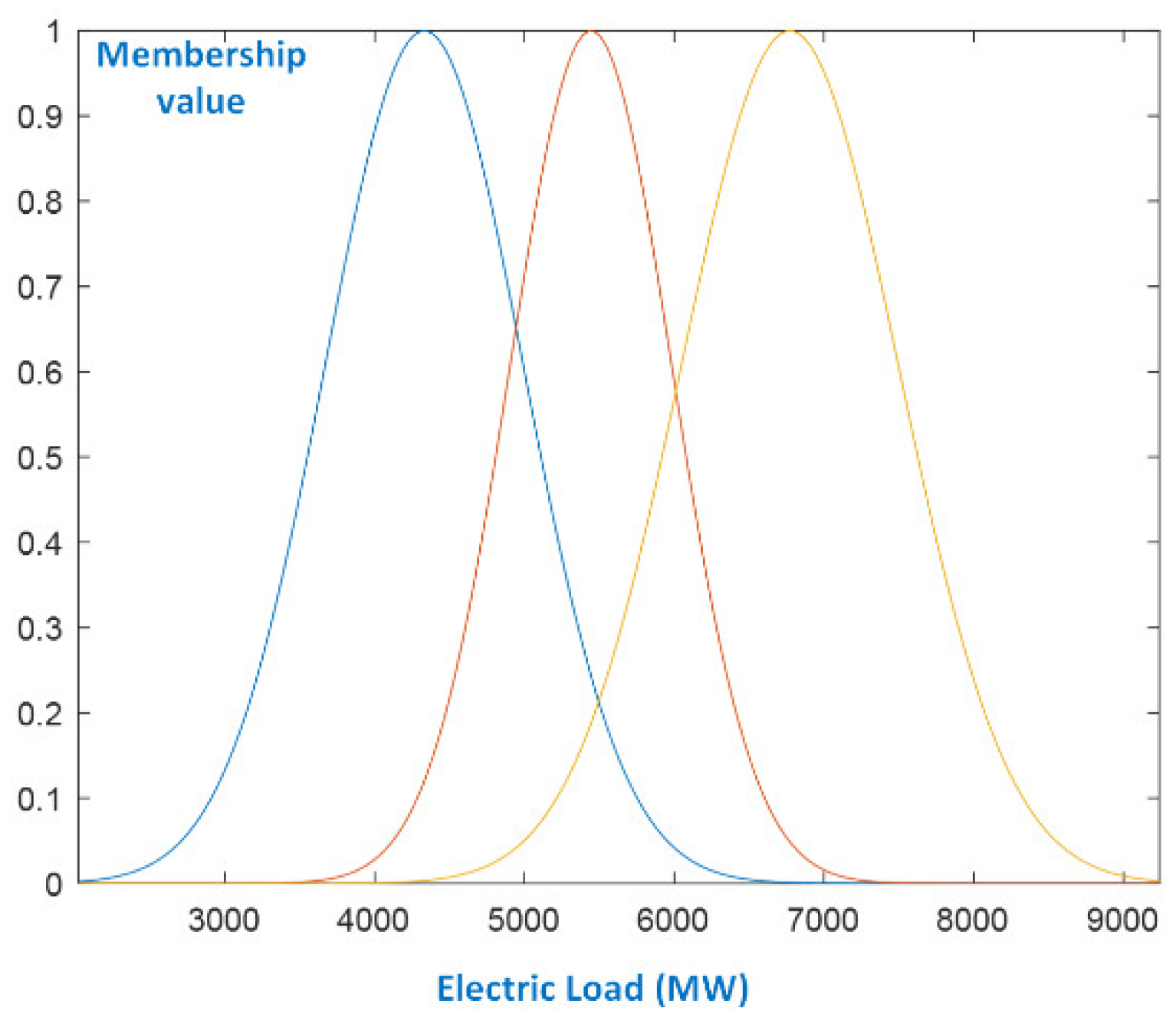
• The fuzzy sets are implemented by Gaussian membership functions as follows:

$$\begin{array}{ccc}{\mu }_{A_j^i}(x_j(n))=\exp \left\{-\frac{1}{2}\cdot \frac{{(x_j(n)-m_{ij})}^2}{{\sigma }_{ij}^2}\right\}& i=1,\dots ,r,& j=1,\dots ,m\end{array}$$

(2)

• The tuning parameters of the premise parts are the mean values, $m_{ij}$, and the standard deviations, ${\sigma }_{ij}$, of the membership functions. It becomes evident from Equation (2) that the premise parts of the fuzzy rules are of a static nature.
• The degree of fulfillment of each rule is the algebraic product of the Gaussian membership functions:

$$\begin{array}{cc}\hfill {\mu }_i(n)=& {\displaystyle \prod _{j=1}^m{\mu }_{A_j^i}(x_j(n))}={\displaystyle \prod _{j=1}^m\exp \left\{-\frac{1}{2}\cdot \frac{{(x_j(n)-m_{ij})}^2}{{\sigma }_{ij}^2}\right\}}=\hfill \\ & \exp \left\{-\frac{1}{2}\cdot {\displaystyle \sum _{j=1}^m\frac{{(x_j(n)-m_{ij})}^2}{{\sigma }_{ij}^2}}\right\}=f\left(\mathit{x}\left(n\right),m_{i1},\dots ,m_{im},{\sigma }_{i1},\dots ,{\sigma }_{im}\right)\hfill \end{array}$$

(3)

• Equation (3) is an m-dimensional Gaussian function. Therefore, the degree of fulfillment corresponds to the membership function of a fuzzy hyper-region. The fuzzy rule-base partitions the input space into operating regions, where each rule can be considered as a local sub-model, which contributes to the overall fuzzy system’s output according to the degree of fulfillment, and produces its own output as a result of the operation of its BDRNN.
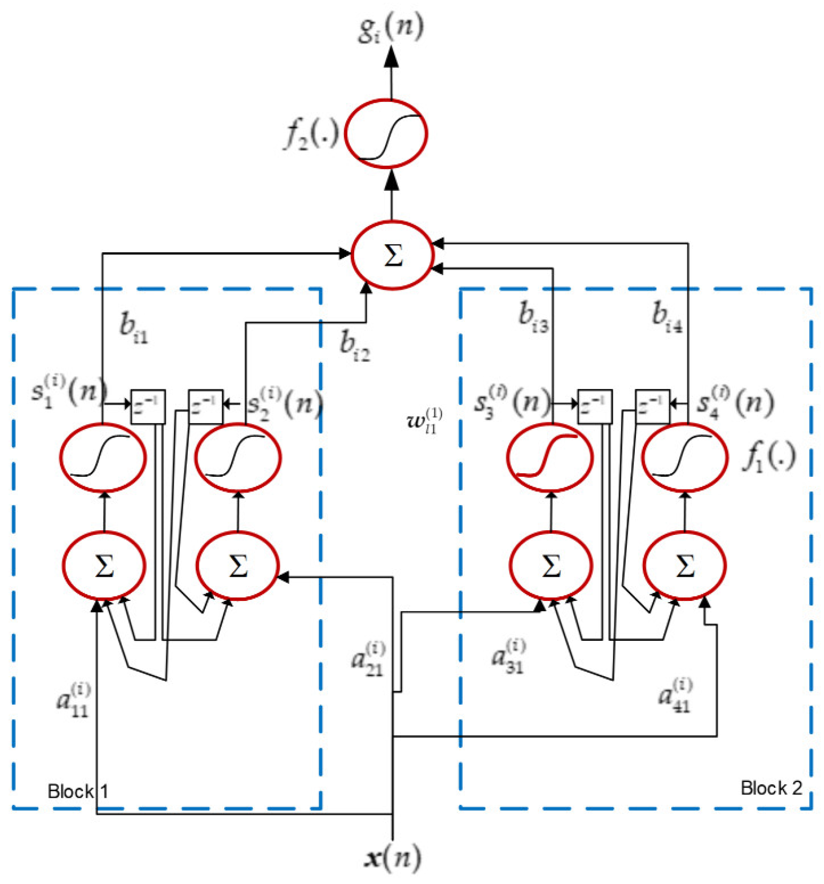
• The consequent parts of the rules are block-diagonal recurrent neural networks. The structure of a two-block BDRNN is presented in Figure 1. The input signal is fed to the blocks of neurons, where each block contains a pair of neurons. There are no connections between neurons that belong to different blocks, while neurons of the same block feedback both to themselves and to each other, with unit delays. This network structure is of a dynamic nature, having internal recurrence (local output feedback, [30]).
  For a BDRNN with N neurons, the outputs of the neurons are given by the following state equations:

  $$s_{2k-1}^{(i)}(n)=f_1\left[{\displaystyle \sum _{j=1}^m{a}_{2k-1,j}^{(i)}\cdot x_j(n)+w_{1,k}^{(i)}\cdot s_{2k-1}^{(i)}(n-1)}+w_{2,k}^{(i)}\cdot s_{2k}^{(i)}(n-1)\right]$$

  (4)

  $$s_{2k}^{(i)}(n)=f_1\left[{\displaystyle \sum _{j=1}^m{a}_{2k,j}^{(i)}\cdot x_j(n)-w_{2,k}^{(i)}\cdot s_{2k-1}^{(i)}(n-1)}+w_{1,k}^{(i)}\cdot s_{2k}^{(i)}(n-1)\right]$$

  (5)

  $i=1,\dots ,r, k=1,\dots ,\frac{N}{2}$.
  The output of the BDRNN for the i-th fuzzy rule is calculated as follows:

  $$g_i(n)=f_2\left[{\displaystyle \sum _{j=1}^N{b}_{ij}\cdot s_j^{(i)}(n)}\right]$$

  (6)

  where the notation given below is used:

  ➢

  The typical sigmoid function, $f\left(z\right)=\frac{1-e^{-z}}{1+e^{-z}}$, implements the activation functions $f_1$ and $f_2$.

  ➢

  $s_{2k-1}^{(i)}(n)$ and $s_{2k}^{(i)}(n)$ are the outputs of neurons that form the k-th block when the n-th sample is processed.

  ➢

  $g_i(n)$ is the output of the i-th fuzzy rule.

  ➢

  $a_{2k-1,j}^{(i)}$ and $a_{2k,j}^{(i)}$ are the synaptic weights of the neurons that form the k-th block, and j is the dimension index of the input vector.

  ➢

  $b_{ij}$ are the synaptic weights of the output neuron.

  ➢

  $w_{1,k}^{(i)}, w_{2,k}^{(i)}$ are the feedback weights of the k-th block of neurons of BDRNN. In order to reduce the number of tuning parameters by half, the scaled orthogonal form is selected. As described in [24], the feedback weights of each block comprise the following feedback matrix:

$$W_k^{(i)}=\left[\begin{array}{cc}{w}_{1,k}^{(i)}& w_{2,k}^{(i)}\\ -w_{2,k}^{(i)}& w_{1,k}^{(i)}\end{array}\right],\hspace{1em}k=1,\dots ,\frac{N}{2}$$

(7)

• The defuzzification part of DBD-FELF produces the model’s output. The weighted average defuzzification scheme is employed, since it is the most popular in TSK fuzzy models, requiring a low computational burden:

$$y(n)=\frac{{\displaystyle \sum _{i=1}^r{\mu }_i(n)\cdot g_i(n)}}{{\displaystyle \sum _{i=1}^r{\mu }_i(n)}}$$

(8)

The architecture of DBD-FELF belongs to a class of dynamic fuzzy neural models where dynamics exist only at the consequent parts of the rules, leaving the premise and defuzzification parts static [31,32]. Moreover, there are no external feedback connections that blur the interpretability of the overall model. This class aims to preserve the local character of TSK modeling, since the rules in these models can be considered as local subsystems that are interconnected through the defuzzifier. The advantages of this class over models with (a) feedback of the total output [33], (b) recurrence in the premise parts of the fuzzy rules [34], or (c) recurrent modules in a cascade connection [35] are highlighted in [36,37,38]. In [39], a similar recurrent neurofuzzy system was introduced as a very efficient load forecaster, having reduced complexity compared to its Deep Learning counterparts. In this context, DBD-FELF is an alternative approach in this path.

3. The Model-Building Process

In the model-building process, the fuzzy rule base is constructed by partitioning the input space, and the forecaster’s parameters are calculated. In an attempt to create a moderately sized fuzzy rule base, the Fuzzy C-Means (FCM) (Dunn [40] and Bezdek [41]) clustering method is applied in order to explore the input space and extract the most appropriate clusters that will determine (a) the number of fuzzy rules and (b) the fuzzy hyper-region of the premise parts.

FCM is a distance-based clustering method, which provides the most appropriate cluster centers in terms of minimum distances between the data samples that belong to each cluster. Since each cluster center corresponds to a fuzzy hyper-region, the resulting clusters produce fuzzy rules so that each one of them is focused on a part of the data set. For a given number of clusters, r, and a data set of P m-dimensional samples, the cluster centers are derived as follows:

$$\begin{array}{ccc}{m}_{ij}=\frac{{\displaystyle \sum _{n=1}^P{\left(u_{in}(n)\right)}^c\cdot x_j(n)}}{{\displaystyle \sum _{n=1}^P{\left(u_{in}(n)\right)}^c}},& i=1,\dots ,r,& j=1,\dots ,m\end{array}$$

(9)

c is a fuzziness parameter within $\left[1,+\infty \right]$ and $u_{in}$ is the membership degree that the n-th data sample belongs to the i-th cluster:

$$u_{in}=\frac{1}{{{\displaystyle \sum _{k=1}^r\left[\sqrt{{\displaystyle \sum _{j=1}^m{\left(m_{ij}-x_j(n)\right)}^2}}\cdot \sqrt{{\displaystyle \sum _{j=1}^m{\left(m_{kj}-x_j(n)\right)}^2}}\right]}}^{\frac{2}{m-1}}}$$

(10)

According to the above, the number of clusters, r, determines the size of the fuzzy rule base. Using Gaussian membership functions for each input axis, Equation (9) provides their mean values. The standard deviations are calculated as proposed in [42]:

$${\sigma }_{ij}=\frac{{\displaystyle \sum _{n=1}^P{u}_{in}\cdot {\left(m_{ij}-x_j(n)\right)}^2}}{{\displaystyle \sum _{n=1}^P{u}_{in}}}$$

(11)

Once the mean values and the standard deviations of the membership functions are determined, the premise parts of the fuzzy rules remain fixed. Thus, the weights of BDRNNs at the consequent parts remain to be tuned.

The training algorithm for the synaptic weights of BDRNN is RENNCOM [43]. It is a constrained optimization method wherein various constraints regarding the learning process can be incorporated. In the present case, the methods based on gradient descent do not guarantee stable learning since, at the hidden layer of BDRNN, there exist feedback connections. Therefore, a constraint relevant to stable learning can be introduced in the form of an appropriate function, which will be optimized simultaneously with the standard error function. Such an approach was followed in [26], where both the premise and consequent parameters were calculated via RENNCOM. In DBD-FELF, the algorithm is applied only to consequent weights and is briefly presented below.

According to the analysis given in [43], regarding the type of feedback matrices in Equation (7), their eigenvalues should fulfill the following constraint for stability to be ensured:

$$\begin{array}{l}\left|{\lambda }_{ik}\right|\le 1\iff \sqrt{{\left(w_{1,k}^{(i)}\right)}^2+{\left(w_{2,k}^{(i)}\right)}^2}\le 1\iff {\left(w_{1,k}^{(i)}\right)}^2+{\left(w_{2,k}^{(i)}\right)}^2\le 1\\ i=1,\dots ,r, k=1,\dots ,\frac{N}{2}\end{array}$$

(12)

A suitable stability function for incorporating Equation (12) is the sigmoid function, which is smooth and continuously differentiable, therefore making it robust to problems caused by parasitic oscillations. Thus, the stability function is written as follows:

$$p_{ik}=f_d(z_{ik})=\frac{1-e^{-a_s\cdot \left({\left|{\lambda }_{ik}\right|}^2-1\right)}}{1+e^{-a_s\cdot \left({\left|{\lambda }_{ik}\right|}^2-1\right)}}=\frac{1-e^{-a_s\cdot \left[{\left(w_{1,k}^{(i)}\right)}^2+{\left(w_{2,k}^{(i)}\right)}^2-1\right]}}{1+e^{-a_s\cdot \left[{\left(w_{1,k}^{(i)}\right)}^2+{\left(w_{2,k}^{(i)}\right)}^2-1\right]}}$$

(13)

The model is stable when the eigenvalues lie within the unit circle. Since parameter $a_s$ controls the slope of the sigmoid function in Equation (13), and consequently, its active region, $a_s$ takes a value within [4,8].

Let all the consequent parameters of Equations (4)–(6) comprise the parameter vector of each fuzzy rule, ${\mathit{\theta }}_{con}$. The RENNCOM algorithm aims to achieve the following three objectives:

(1)

The error measure, E, should be minimized so that the electric load time-series, $\widehat{y}(n)$, is identified. The Mean Squared Error is selected to be the error measure:

$$MSE=\frac{1}{P}\cdot {\displaystyle \sum _{n=1}^P{\left[y(n)-\widehat{y}(n)\right]}^2}$$

(14)

The error measure is minimized through an iterative process, where, at each iteration, $E$ is decremented by a certain amount, $\delta E$. This change is selected in an adaptive way so that, after a succession of iterations, the accumulated changes lead to the establishment of an accurate input-output representation.

(2)

A second function, called the pay-off function, Φ, should be minimized so that stability during the learning process is preserved. In the present case, the pay-off function includes the constraints given by Equation (12) and has the following form:

$$\Phi =\frac{1}{2}\cdot {\displaystyle \sum _{i=1}^r{\displaystyle \sum _{k=1}^{\frac{N}{2}}{\left(-1-p_{ik}\right)}^2}}=\frac{1}{2}\cdot {\displaystyle \sum _{i=1}^r{\displaystyle \sum _{k=1}^{\frac{N}{2}}\left\{\frac{2}{1+e^{-a_s\cdot \left[{\left(w_{1,k}^{(i)}\right)}^2+{\left(w_{2,k}^{(i)}\right)}^2-1\right]}}\right\}}}$$

(15)

From Equation (15), it can be inferred that minimizing Φ means maximizing the denominators and, consequently, forcing the sums ${\left(w_{1,k}^{(i)}\right)}^2+{\left(w_{2,k}^{(i)}\right)}^2-1$ to be negative. Therefore, the consequent weights are updated so that the eigenvalues of the block submatrices lie within the unit circle.

(3)

An extra condition is imposed, which facilitates a search in the weight space [43]:

$${\Phi }_w=d{\mathit{\theta }}^T\cdot {({\Delta }^2)}^{-1}\cdot d\mathit{\theta }-1=0$$

(16)

$d\mathit{\theta }$ is the amount by which the consequent parameter vector is changed at each iteration. Matrix Δ is a diagonal matrix that hosts the maximum parameter change (MPC) of each weight. Equation (16) describes a hyper-ellipsoid, which is centered on the current consequent weight vector, and a search for the new values of the weights is restricted by this hyper-ellipsoid. For given values of $\delta E$ and Δ, the optimal $d\mathit{\theta }$ is the vector that maximizes $d\mathit{\Phi }$.

An analysis of the consequent updates in the parameters is fully described in [43]. The set of equations that implement the learning scheme is as follows:

$${\mathit{\theta }}_{new}={\mathit{\theta }}_{old}+d\mathit{\theta }$$

(17)

$$\begin{array}{cc}\hfill d\mathit{\theta }=& -{\Delta }^2\cdot \sqrt{\frac{\left[{\left(\frac{\partial E}{\partial \mathit{\theta }}\right)}^T\cdot {\Delta }^2\cdot \frac{\partial E}{\partial \mathit{\theta }}\right]-{(\delta E)}^2}{\left[{\left(\frac{\partial \Phi }{\partial \mathit{\theta }}\right)}^T\cdot {\Delta }^2\cdot \frac{\partial \Phi }{\partial \mathit{\theta }}\right]\cdot \left[{\left(\frac{\partial E}{\partial \mathit{\theta }}\right)}^T\cdot {\Delta }^2\cdot \frac{\partial E}{\partial \mathit{\theta }}\right]-{\left[{\left(\frac{\partial \Phi }{\partial \mathit{\theta }}\right)}^T\cdot {\Delta }^2\cdot \frac{\partial E}{\partial \mathit{\theta }}\right]}^2}}\hfill \\ & \cdot \left[{(\frac{\partial \Phi }{\partial \mathit{\theta }})}^T-{\left(\frac{\partial E}{\partial \mathit{\theta }}\right)}^T\cdot \frac{{\left(\frac{\partial \Phi }{\partial \mathit{\theta }}\right)}^T\cdot {\Delta }^2\cdot \frac{\partial \Phi }{\partial \mathit{\theta }}}{{\left(\frac{\partial E}{\partial \mathit{\theta }}\right)}^T\cdot {\Delta }^2\cdot \frac{\partial E}{\partial \mathit{\theta }}}\right]+{\Delta }^2\cdot {\left(\frac{\partial E}{\partial \mathit{\theta }}\right)}^T\cdot \frac{\delta E}{{\left(\frac{\partial E}{\partial \mathit{\theta }}\right)}^T\cdot {\Delta }^2\cdot \frac{\partial E}{\partial \mathit{\theta }}}\hfill \end{array}$$

(18)

The decrement $\delta E$ is expressed as a function of the gradient $\frac{\partial E}{\partial \theta }$, the MPC matrix, and a constant ξ within [0, 1]:

$$\delta E=-\xi \cdot \left[{\left(\frac{\partial E}{\partial \mathit{\theta }}\right)}^T\cdot {\Delta }^2\cdot \frac{\partial E}{\partial \mathit{\theta }}\right]$$

(19)

Due to the dynamic nature of the neurons and the existence of temporal relations, the gradients $\frac{\partial E}{\partial \mathit{\theta }}$ and $\frac{\partial \Phi }{\partial \mathit{\theta }}$ are extracted using ordered derivatives [44] and Lagrange multipliers, which facilitate the process. Moreover, the multipliers with respect to the feedback weights create difference Equations (21) and (23), which are solved recursively, starting from the last data sample (Equations (22) and (24)):

$${\lambda }_{g,i}(n)=\frac{2}{P}\cdot (y(n)-\widehat{y}(n))\cdot \frac{{\mu }_i(n)}{{\displaystyle \sum _{j=1}^r{\mu }_j(n)}}$$

(20)

$$\begin{array}{cc}\hfill {\lambda }_{s,2k-1}^{(i)}(n)& ={\lambda }_{g,i}(n)\cdot b_{i,2k-1}\cdot f_2^{\prime }(n,i)+{\lambda }_{s,2k-1}^{(i)}(n+1)\cdot w_{1,k}^{(i)}\cdot f_1^{\prime }(n+1,i,2k-1)\hfill \\ & -{\lambda }_{s,2k}^{(i)}(n+1)\cdot w_{2,k}^{(i)}\cdot f_1^{\prime }(n+1,i,2k)\hfill \end{array}$$

(21)

$${\lambda }_{s,2k-1}^{(i)}(P)={\lambda }_{g,i}(P)\cdot b_{i,2k-1}\cdot f_2^{\prime }(P,i)$$

(22)

$$\begin{array}{cc}\hfill {\lambda }_{s,2k}^{(i)}(n)& ={\lambda }_{g,i}(n)\cdot b_{i,2k}\cdot f_2^{\prime }(n,i)+{\lambda }_{s,2k-1}^{(i)}(n+1)\cdot w_{2,k}^{(i)}\cdot f_1^{\prime }(n+1,i,2k-1)\hfill \\ & +{\lambda }_{s,2k}^{(i)}(n+1)\cdot w_{1,k}^{(i)}\cdot f_1^{\prime }(n+1,i,2k)\hfill \end{array}$$

(23)

$${\lambda }_{s,2k}^{(i)}(P)={\lambda }_{g,i}(P)\cdot b_{i,2k}\cdot f_2^{\prime }(P,i)$$

(24)

$f_1^{\prime }(n+1,i,2k-1)$, $f_1^{\prime }(n+1,i,2k)$, and $f_2^{\prime }(n,i)$ are the derivatives of the neurons of the hidden and output layers, with respect to their arguments.

At each iteration, each consequent parameter update, $d{\theta }_i$, varies from the other updates since it fulfills the constraint $\left|d{\theta }_i\right|\le {\Delta }_i$. The MPCs are adaptable, and their values are changed via the following adaptation mechanism: Initially, all the consequent weights take a value ${\Delta }_0$. The gradients of E with respect to each weight $d{\theta }_i$ at the present and the previous iterations are monitored, and their product is calculated. If the product is positive, MPC increases by a factor $n^{+}\in \left[1.1, 1.3\right]$, else it diminishes by a factor $n^{+}\in \left[0.5, 0.8\right]$. The MPCs are bounded by a small positive number in the range ${10}^{-5}-{10}^{-3}$ so that the weights retain nonzero values.

According to the above, at each iteration, the learning process involves the following steps: First, the aforementioned adaptation mechanism calculates the new MPCs. Next, the consequent parameters are updated using Equations (17)–(24), and the current MSE is calculated. If a predefined threshold for MSE is attained, the learning process ends; otherwise, it is repeated. The whole model-building process is depicted by the flow-chart in Figure 2.

4. Experimental Results

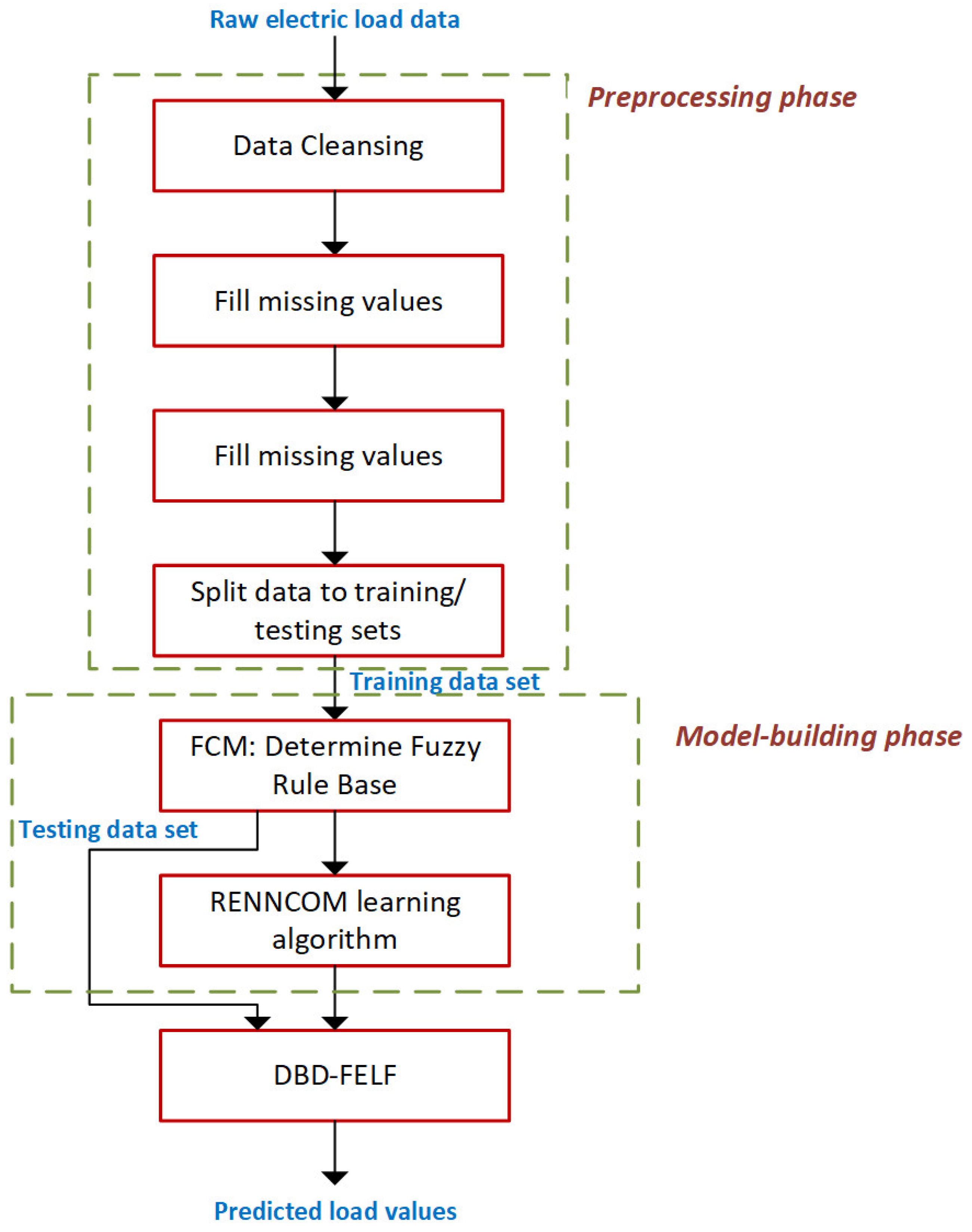
4.1. Problem Statement—Data Preprocessing Phase

The DBD-FELF described in the previous section is applied to predict one-day-ahead hourly loads of the Greek power system. In an attempt to investigate whether a recurrent system is capable of identifying the temporal relations of the electric load time-series, two decisions were made regarding the forecasting scenario:

(a)

The data set is not divided into seasons and the whole annual electric load time-series is examined. Moreover, there is no separation between working days and weekends.

(b)

A single input is used—the actual load value at hour h of the previous day, ${\widehat{L}}_{d-1,h}$ (MW)—with DBD-FELF predicting the load at the same hour of day d. In this way, the forecaster attempts to identify the mapping

$$L_{d,h}=f\left({\widehat{L}}_{d-1,h}\right)$$

(25)

without resorting to climate and temperature variables. d = 1, …, 365 and h = 1, …, 24 are the day and hour indices, respectively. This decision is made to provide a very economical model in terms of parameters and computational burden. Therefore, no feature selection (a rather demanding preprocessing step) is required based either on the expertise of the system operators or on statistical methods and regression models [45]. DBD-FELF intends to model the dependence of current load on past loads by taking advantage of the recurrent nature of BDRNNs.

Two error measures are selected in order to evaluate the forecasting performance of DBD-FELF. The first one is the Root Mean Squared Error, which is the root of MSE (Equation (14)). It is the most common metric in the area of modeling, measuring, in a quadratic manner, the discrepancy between the actual data and the output of the forecaster.

The second metric is the Average Percentage Error (APE) with respect to the daily peak:

$$APE=\frac{1}{M}{\displaystyle \sum _{d=1}^M\left[\frac{1}{24}\cdot {\displaystyle \sum _{h=1}^{24}\frac{\left|L_{d,h}-{\widehat{L}}_{d,h}\right|}{L_{\max ,d}}}\right]\cdot 100\%}$$

(26)

where M is the number of days in the data set and ${\widehat{L}}_{\max ,d}$ is the maximum actual load of day d.

The data set contains hourly load values from four consecutive years, 2013–2016, which are publicly available on the Greek Independent Power Transmission Operator website [46]. The total amount of data (35,064 samples) is split into training and testing data sets by a ratio of 3 to 1, respectively. The first three years constitute the training data set (26,280 samples), and the leap year, 2016, which contains 8784 samples, is the testing set. A preprocessing stage was necessary to deal with missing or irregular values, integrate the data in a common format, and perform normalization so that they can be used by BDRNNs. When a missing or irregular value occurred, it was filled by the average of the value at the same hour of the previous day and the next one. When there were consecutive missing values, cubic spline interpolation was employed to fill the gaps.

As far as normalization is concerned, data are within $\left[-0.8, 0.8\right]$, meaning that load data fall within the slopes of the activation function of the neurons at the consequent parts of the fuzzy rules.

The final data file contains 1461 lines (three regular years and one leap year) and 25 feature columns (one for the data serial number and twenty-four for the hourly loads). Apart from these columns, some more were added, containing metadata regarding the day of the week and season of the year. These additions were necessary in order to perform evaluation tests, partition the results into seasonal data or to working days and weekends, etc.

4.2. DBD-FELF’s Features

The tuning parameters of a DBD-FELF, with Gaussian membership functions, r rules, and N hidden neurons at each rule, are hosted in

Table 1. Parameters of DBD-FELF.

Parameter	Number
m	r
σ	r
a	r·N
b	r·N
w	r·N
Premise	2·r
Consequent	3·r·N
Total	2·r +3·r·N

.

The FCM partition algorithm leads to a fuzzy rule base with 3 rules. It should be noted that the same dataset used in [39] is employed; therefore, the conclusions regarding the selection of the number of rules based on the Davies–Bouldin index [47] and the respective arguments apply here as well. Please refer to [39] for a detailed analysis. Moreover, since a comparative analysis with the forecaster proposed in [39] is presented in the sequel, the same input partition facilitates the comparison. The input space partition is presented in Figure 3.

It can be concluded from Figure 3 that the three fuzzy sets adequately cover the input space, which is centered at 4306, 5428, and 6751 MW, meaning that the three cluster centers are placed where the load values appear most of the time. The first and third fuzzy sets have Gaussian membership functions with higher standard deviations than the set in the middle in an attempt to cover the lower and upper values of the universe of discourse. As far as overlapping is concerned, the first and second fuzzy sets have an overlapping factor of 65%, and the second and third sets have an overlapping factor of 59%. Moreover, in the central region of loads, all three rules operate with an overlapping factor of 22% between the first set and the third one. These high overlapping factors are necessary for the rules to operate cooperatively in a wide range of electric loads.

BDRNNs with 1 to 5 blocks were examined. As shown in Section 4.3, a single block is sufficient to accurately perform predictions. Therefore, N is set to 2, and the parameter set is limited to 24 parameters. Since the premise parameters are determined by Equations (9) and (11), only 18 consequent weights (75% of the total number of parameters) need to be tuned by RENNCOM.

The learning parameters of RENNCOM are shown in

Table 2. Learning parameters of RENNCOM.

${\mathit{n}}^{+}$	${\mathit{n}}^{-}$	${\mathbf{\Delta }}_{\mathbf{min}}$	${\mathbf{\Delta }}_{\mathbf{max}}$	${\mathbf{\Delta }}_{\mathbf{0}}$	${\mathit{a}}_{\mathit{s}}$	$\mathit{\xi }$	Iterations
1.05	0.5	1 × 10−4	0.5	1 × 10−2	6	0.9	1000

.

4.3. Experimental Results

In order to depict the effect of network complexity to forecasting performance, the yearly forecast APE and RMSE, attained by DBD-FELFs with 1 to 5 blocks of recurrent neurons in their consequent parts of their rules, are summarized in

Table 3. Yearly APE and RMSE.

No of Blocks	APE Training	RMSE Training	APE Testing	RMSE Testing	No of Param.
1	1.05%	107	1.18%	112	24
2	1.10%	104	1.22%	110	42
3	1.09%	107	1.20%	110	60
4	1.05%	107	1.18%	111	78
5	1.13%	108	1.18%	108	96

. The RMSE is calculated on the denormalized (actual) values and is expressed in MW. All the results are averaged over 10 trials. Taking into consideration that, usually, an electric load prediction is considered reliable when its APE value falls below 2%, it becomes evident that all five versions of DBD-FELF operate very effectively. Moreover, the existence of internal feedback at each rule and the efficient partition of the input space are reflected on the size of BDRNN necessary for a fuzzy rule to track the time-series dynamics. The simplest BDRNN performs practically the same compared to bigger networks; therefore, in the sequel, the DBD-FELF with a single block of recurrent neurons will be employed.

The seasonal forecasting results are reported in

Table 4. Seasonal APE and RMSE.

Season	APE Training	RMSE Training	APE Testing	RMSE Testing
Winter	1.03%	125	1.04%	121
Spring	1.36%	118	1.66%	131
Summer	0.81%	90	0.96%	104
Autumn	1.00%	88	1.03%	88

. Despite the fact that a single model is used for the whole year, DBD-FELF predicts well below 2% in all seasons, with Spring being the most difficult season, where the highest deviation between the training and the testing error values occurs. The behavior of the forecaster is very similar for the three remaining seasons, with APE values vary in a very small range, 0.08%.

In terms of the absolute error for the testing data set, a yearly average of 76.2 MW is attained, with its standard deviation being 81.8 MW, which means that the forecast error is less than 158 MW for most of the hours in 2016 (8784 h as it was a leap year). The absolute error duration curve is hosted in

Table 5. Absolute error duration curve.

Electric Load	>100 MW	>200 MW	>400 MW	>500 MW
Hours	2686	718	62	15
Time	30.58%	8.17%	0.70%	0.18%

. This curve depicts the percentage of hours of the year in which the absolute value of the forecast error is greater than the values given in the first row. It becomes evident that DBD-FELF performs very efficiently since, for nearly 69.5% and 92% of the time, the forecast error is less than 100 and 200 MW, respectively. Moreover, the forecast error exceeds 500 MW for 15 h throughout the year. It should be noted that 9 out of these 15 h belong to Orthodox Easter and Assumption days, which are highly irregular days, as will be discussed in the sequel.

The daily evolution of electric load for weekdays and Sundays, regarding all seasons, is shown in Figure 4, Figure 5, Figure 6 and Figure 7, and a winter week is hosted in Figure 8. Moreover, Figure 9 presents the three major holidays in Greece: Christmas, Orthodox Easter, and Assumption days. In these charts, the blue solid lines are the actual load data series, and the red dashed lines refer to the predictions made by DBD-FELF.

From Figure 4, Figure 5, Figure 6, Figure 7, Figure 8 and Figure 9, the following observations can be made:

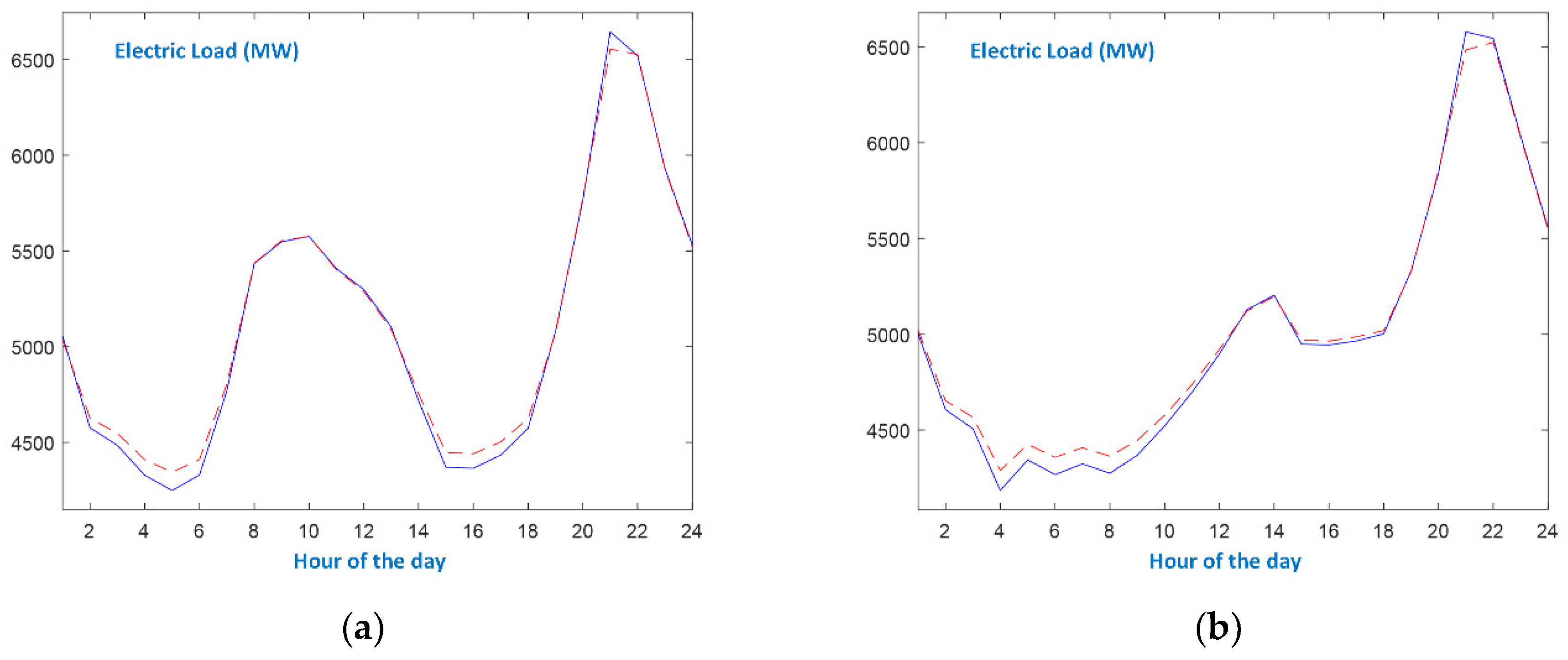
• In the case of working days, the appearances of morning and evening peaks, as well as the first minimum load, are similar at all seasons. During Spring and Autumn working days, the evening minimum is more discrete than during Winter and Summer.
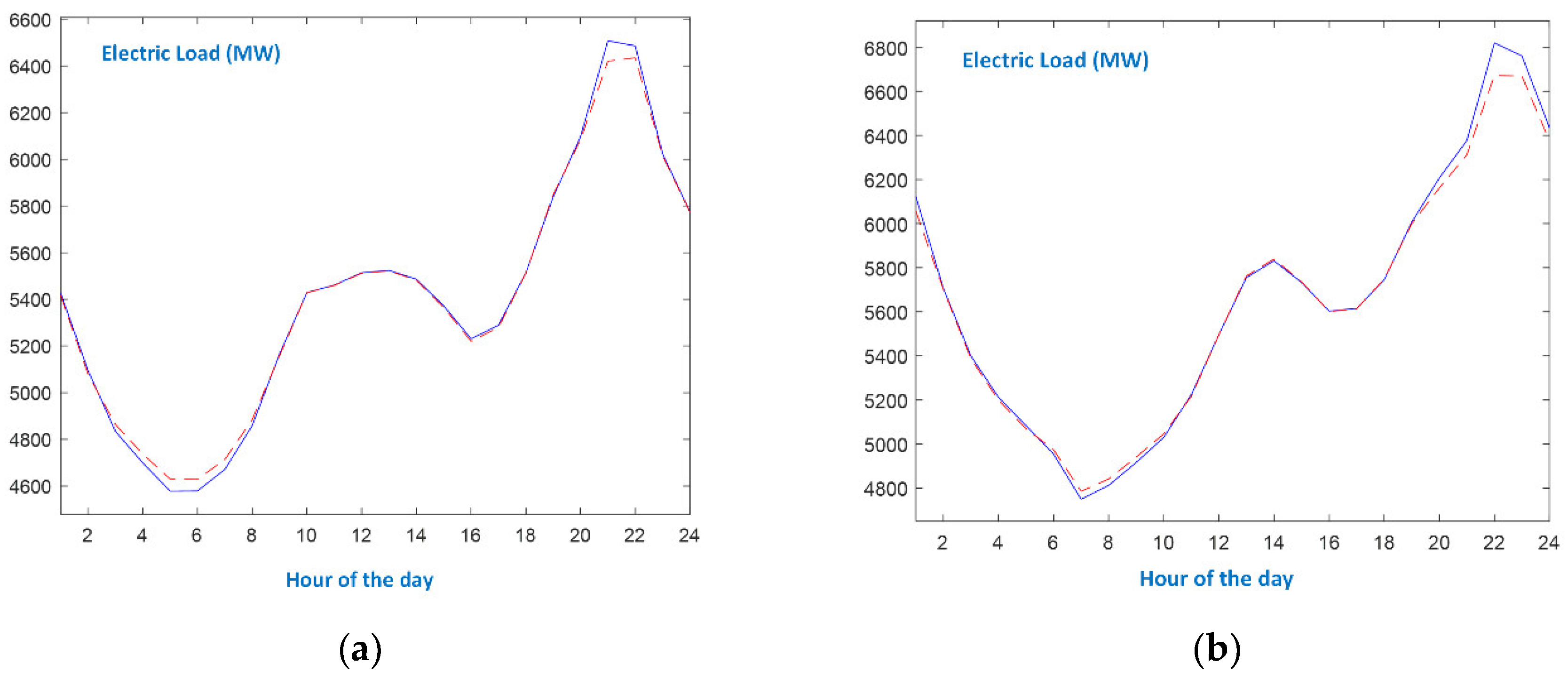
• As expected, the evolution of the load curve on Sundays is quite different from the one of working days. Additionally, the seasonal patterns are also different. Autumn and Spring Sundays follow the evolution of the respective working day load curves after 6 p.m.
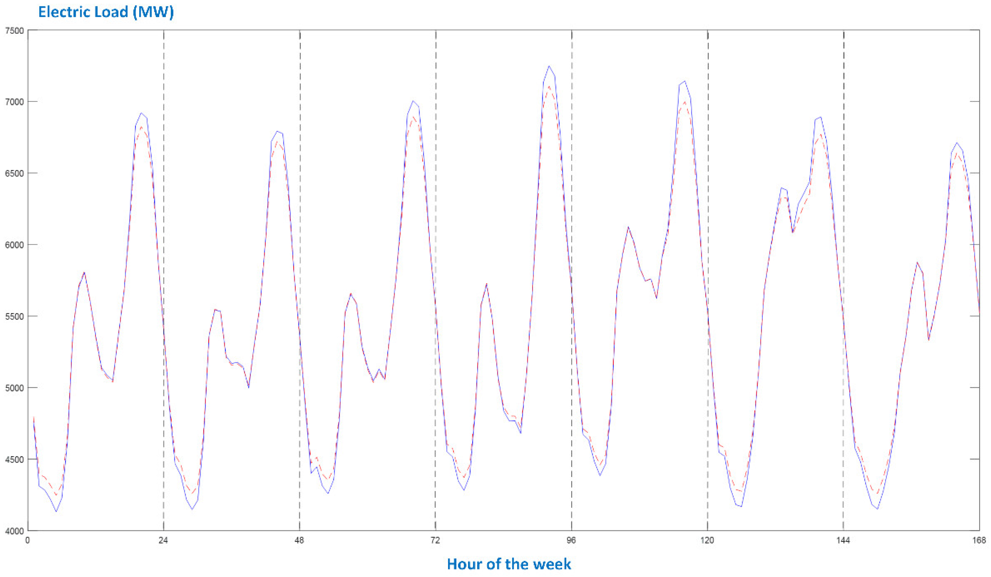
• Even though there exist differences between seasonal patterns, as well as between the types of days, the proposed forecaster efficiently models the actual load curves since it identifies the peaks and the minimum loads and accurately predicts the values at the slopes. As shown in Figure 8, the single-input forecaster is capable of tracking the transition from weekend days to working days and vice versa.
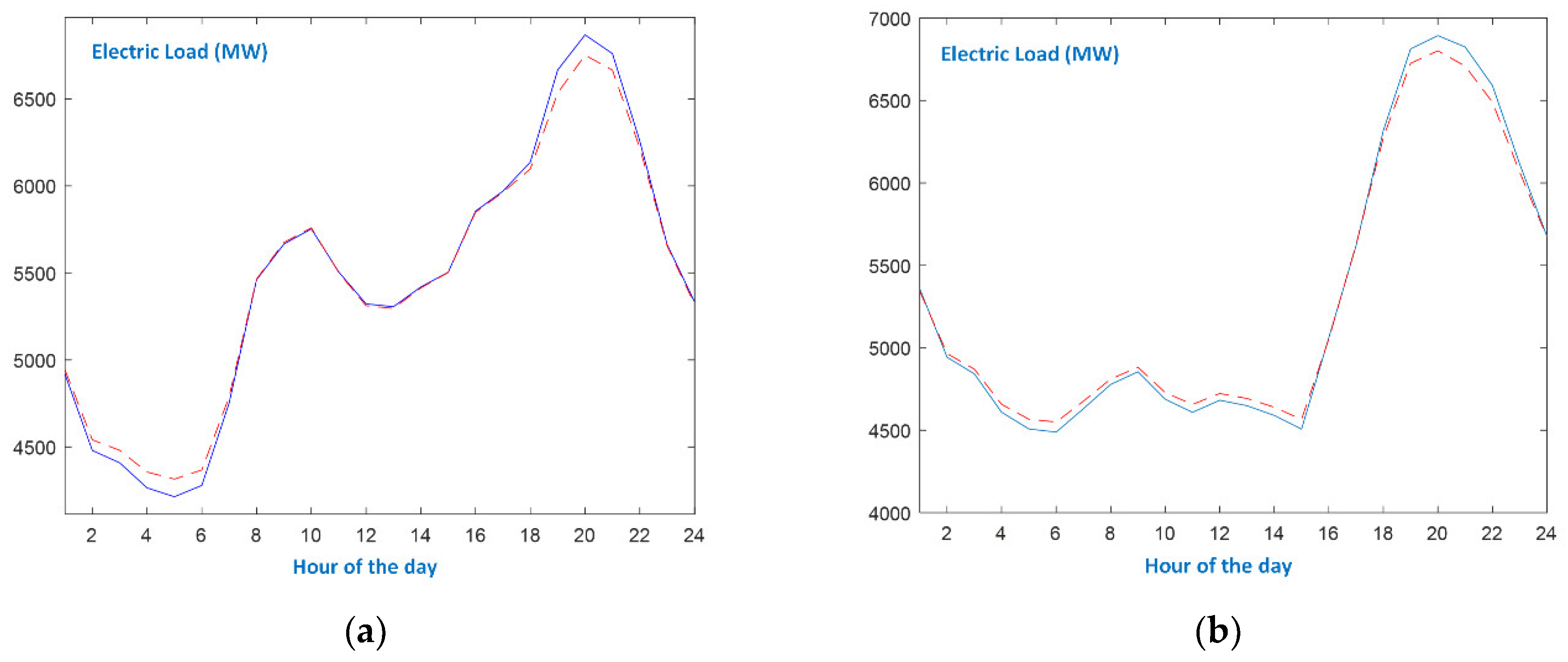
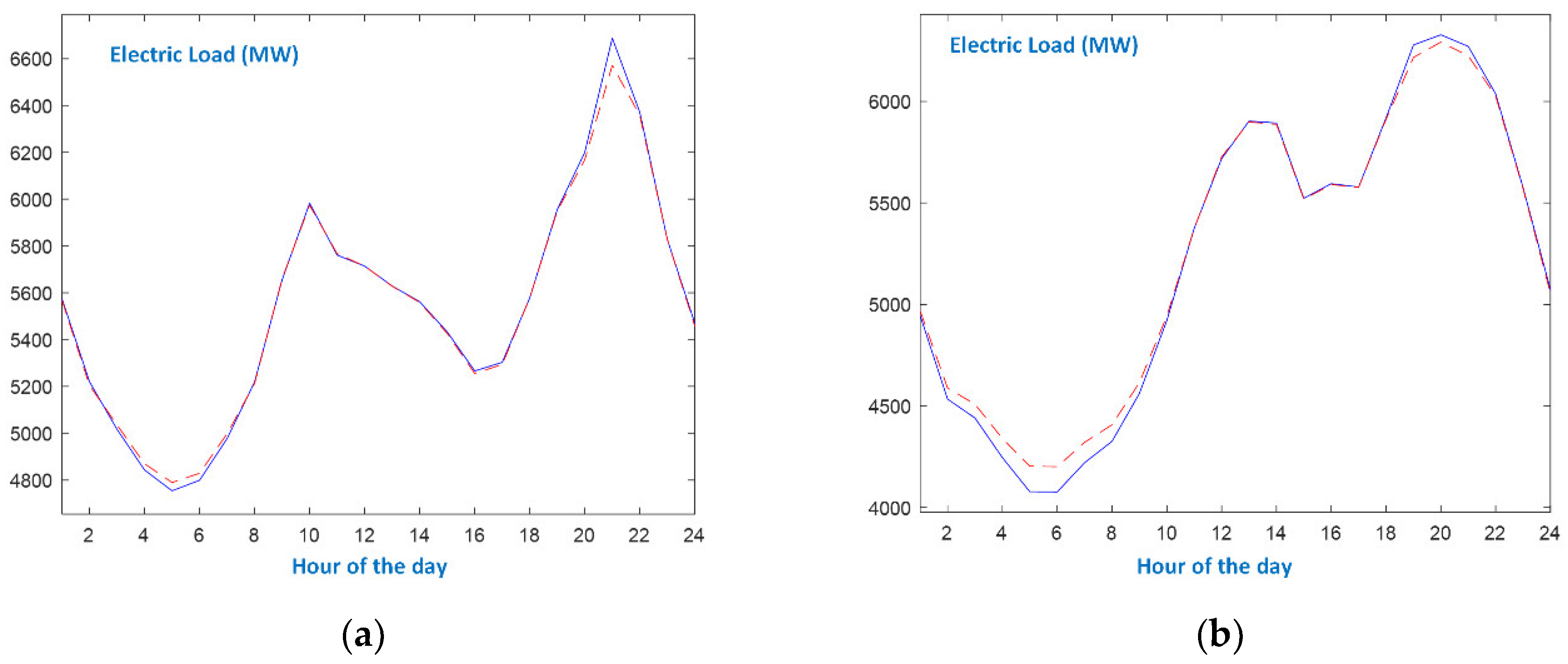
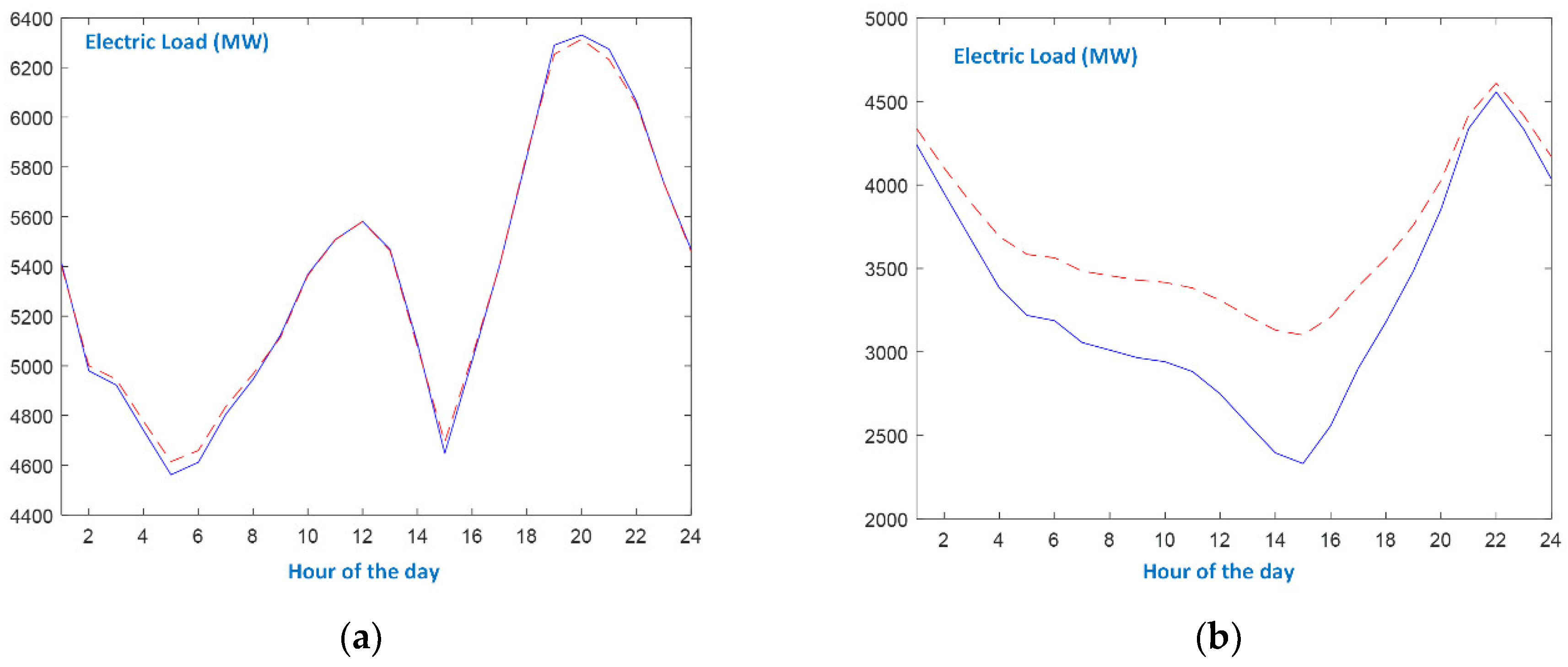
• As far as Holidays are concerned, it can be seen in Figure 9a that the Christmas load curve is tracked by DBD-FELF very efficiently. The average percentage error for Christmas day is 0.31%. This behavior can be attributed to the fact that, during Christmas, Greeks stay at home or pay visits; therefore, the household loads compensate the industrial ones. The two minima occur at 5 a.m. and 3 p.m., and the first peak load at 10 a.m., at the same hours as the previous day. Moreover, the load evolution is quite similar on these two days, leading to the conclusion that the temporal relation of past loads has been effectively identified.
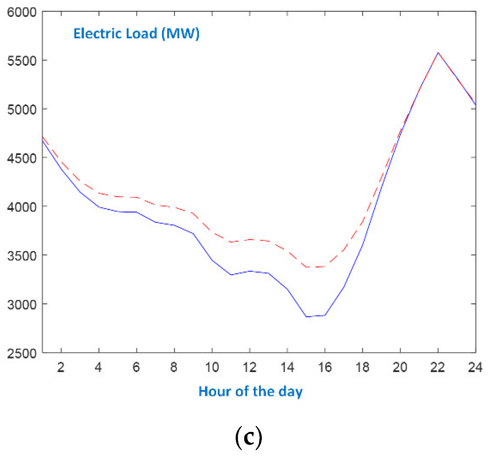
• On the contrary, the Easter and Assumption holidays are quite a different story. The day of Easter is a highly irregular day, as shown in Figure 9b. There is no morning peak, and there is a continuous decrease in load demand until 3 p.m. Moreover, the load values are significantly reduced (2331 MW at 3 p.m.) with respect to the previous day (3405 MW) and to the previous Sunday (3392 MW), leading to enormous errors, including the following: 735.9 MW at 2 p.m., 770 MW at 3 p.m. and 652.6 at 4 p.m., and an average percentage error of 8.11%. This unusual load curve reflects the fact that, during Easter, no industrial activity takes place, and Greek people leave their homes and celebrate outdoors. The evening peak attains 4500 MW, whereas, in a typical Spring Sunday, the respective peak is around 6500 MW (Figure 5b). In the case of 15 August (Assumption day), DBD-FELF is not accurate, at least until 6p.m. Even though it tracks the dynamics, the predicted load takes fairly bigger values, leading to errors up to 507 MW. The load curve is quite similar to that of Easter, as there is no morning peak as well, and load keeps more or less reducing to a minimum below 3000 MW around 3 p.m. (lunch time). Assumption day is at the heart of summer vacations for Greek people; most are on leave and spend the morning at the beach, returning to their summer houses or to hotels late in the evening. However, the load profile returns to normal at around 6 p.m., and the performance DBD-FELF is significantly ameliorated. The average percentage error for 15 August is 3.53%.

DBD-FELF is tested in comparison to six Computational Intelligence-based static and dynamic models, namely, ANFIS [48], LSTM forecaster [45,49], GRU and RNN models [17], the DFNN [36], and the ReNFuzz-LF [39] neurofuzzy models. ANFIS is selected as a well-established static neurofuzzy system, LSTM is an effective Deep Learning model in modeling applications, and GRU and Recurrent Neural Networks are popular dynamic schemes with enhanced learning capabilities. The pool of competing rivals includes two dynamic neurofuzzy systems, DFNN and ReNFuzz-LF, which are based on generalized TSK fuzzy rules such as DBD-FELF but have different network structures of the consequent parts, as described in [39]. The criteria employed in the comparative analysis are the prediction accuracy and model complexity. All models are applied to the same data sets of the Greek power system. Several setups of the LSTM scheme are tested: networks with one and two layers, each layer consisting of 25, 50, or 500 units. The results from four of them are included below, having been averaged over 10 trials. A GRU with two layers and 500 units per layer, along with two RNNS with two hidden layers and 40/200 neurons per layer, respectively, are also included in the test pool. Their other hyperparameters are summarized in

Table 6. Parameters of the competing forecasters.

DFNN	Structural Parameters
$O_u$	$O_{y_1}$	$O_{y_2}$	$O_{y_3}$	H	Membership function	Activation function
1	2	2	1	2	Gaussian	tanh
Learning parameters
$n^{+}$	$n^{-}$		${\Delta }_{\min }$		${\Delta }_0$	$\xi$
1.05	0.5		0.0001		0.01	0.85
ReNFuzz-LF	Structural Parameters
H	Membership function			Activation function
2	Gaussian			tanh
Learning parameters
Temp	$a_1$	$a_2$	$n^{+}$	$n^{-}$	${\Delta }_{\min }$	${\Delta }_0$
1.2	0.01	0.4	1.05	0.5	0.0001	0.01
ANFIS	Learning parameters
Initial Step size	Step size increase rate			Step size decrease rate
0.01	1.1			0.9
Membership function: Gaussian
GRU	Hyperparameters
Activation function	Bias	Dropout	Batch size	Optimizer		learning rate
tanh	Yes	0.35	16	Adam		0.001
LSTM-1	Hyperparameters
Activation function	Bias	Dropout	Batch size	Optimizer		learning rate
tanh	Yes	0.35	16	Adam		0.001
LSTM-2,3,4	Hyperparameters
Activation function	Bias	Dropout	Batch size	Optimizer		learning rate
tanh	Yes	0.2	24	Adam		0.001
RNN-1	Hyperparameters
Activation function	Bias	Dropout	Batch size	Optimizer		learning rate
tanh	Yes	0.35	80	Adam		0.001
RNN-2	Hyperparameters
Activation function	Bias	Dropout	Batch size	Optimizer		learning rate
tanh	Yes	0.35	24	Adam		0.001

, where the structural and learning parameters of DFNN and ReNFuzz-LF are also given—taken from [39]. The FCM partition applied to DBD-FELF is used for DFNN and ReNFuzz-LF. The input vector of the ANFIS model comprises two inputs, $\left[L_{d-1,h},L_{d-1,h-1}\right]$, in an attempt to compensate for its static nature. Among the several ANFIS structures that were investigated, the one containing nine fuzzy sets per input, grid partition, and a fuzzy rule base of eighty-one rules is selected. All forecasters are trained for 1000 iterations. The results are reported in

Table 7. Results of the competing forecasters.

Model	APE (Testing)	No. of Parameters
DBD-FELF	1.18%	24
ReNFuzz-LF	1.35%	33
DFNN	1.36%	48
ANFIS	1.48%	279
LSTM-4 (1 layer, 25 units)	1.73%	2726
RNN-2 (40 neurons)	1.72%	4961
LSTM-3 (1 layer, 50 units)	1.51%	10,451
LSTM-2 (2 layers, 50 units)	1.23%	30,651
RNN-1 (200 neurons)	1.71%	120,801
GRU	1.17%	2,258,001
LSTM-1 (2 layers, 500 units)	1.18%	3,006,501

.

From the aforementioned results, it becomes evident that all seven types of models and all eleven forecasters attained APE values below 2%, with six of them predicting with APE less than 1.40%. DBD-FELF, GRU, and LSTM-1 exhibit a similar performance, with the proposed forecaster requiring a parameter set that is a fraction of those of the other two rivals. Moreover, all three dynamic neurofuzzy forecasters proved to be very efficient despite their small size.

Additionally, recurrent neural networks are the least effective, even with a very complex structure. These observations highlight the following: (a) the advantage that local recurrence offers one tasked with identifying the temporal relations of data series, even with a limited number of units, and (b) the enhanced learning capabilities with low computational complexity that the fuzzy blending of small scale recurrent sub-systems can create. Moreover, DBD-FELF outperforms ReNFuzz-LF in terms of prediction accuracy and structure complexity.

In order to further highlight the characteristics of the tested models, the times required to complete the training and testing phases are given in

Table 8. Duration of the training and testing phases for the forecasters with the best performance.

Model	Training Phase (Seconds)	Testing Phase (Seconds)
DBD-FELF	49.87	0.72
GRU	347.8	7.187
LSTM-1 (2 layers, 500 units)	584.4	8.973

, where the most efficient forecasters are included. All models were executed using Google Colab. Its sessions were initialized with a K80 GPU and 12 GB of RAM. All the results were averaged over 10 trials. According to the reported times, it becomes evident that the small structure of DBD-FELF reflects the duration of the training phase and the fast operation of the resulting system.

Hence, it can be stated that the block-diagonal feedback structure of the consequent parts of the fuzzy rules can model the internal dependencies of the load time-series better than the respective consequent parts of ReNFuzz-LF, which are recurrent neural networks with simple local output feedback. An interesting conclusion can be drawn from the forecast error duration curves of DBD-FELF and ReNFuzz-LF; in Figure 10, the reduction in terms of hours that DBD-FELF has produced over the curve of ReNFuzz-LF is shown. Even though, in the area of 100 MW, the value is very low (just 3.62%), which means that these forecasters practically operate in the same way where their prediction results are most accurate, the difference in the amount of hours increase as less accurate forecasts are produced. For instance, ReNFuzz-LF has 40 h with a prediction error over 500 MW [39], while DBD-FELF has 15 h—showing a 62.50% reduction. The results in Figure 10 show that the proposed forecaster is more robust, preventing large errors.

In conclusion, DBD-FELF has the following characteristics:

• It produces accurate forecasts for the electric load data of the Greek Power System.
• It is an economical model with reduced computational complexity with regard to its rivals.
• The model-building process does not require a preprocessing step for selecting appropriate past load values.
• The model operates effectively without climate variables.
• A single model is applied for forecasting the whole year, independent of the nature of the day. The results justify this decision in general; however, the effect of highly irregular days such as Easter and 15 August (Assumption day) are clear.

5. Conclusions

A block-diagonal fuzzy neural network for short-term electric load forecasting of the Greek power system has been suggested. DBD-FELF is a fuzzy system with rules that have small-scale block-diagonal recurrent structures as consequent parts. Unit feedback connections exist between the pairs of neurons that constitute each block. The FCM clustering method performs the partition of the single input’s space, determining the size of the fuzzy rule base and the values of the premise parameters. The RENNCOM iterative method guarantees stable learning of the consequent weights. Climate and temperature variables are not included in the input vector, while past load values are kept to the minimum. These decisions led to an economical and fast forecaster, while the experimental results have shown that DBD-FELF produces very accurate predictions, equal or superior to Computational Intelligence-based models of significantly higher complexity. Obviously, this approach has limitations regarding performance in cases of highly irregular days, where the load evolution is very different from the one in previous days. In the future, the effect of highly irregular days should be dealt with, possibly by introducing some expert knowledge in the form of typical fuzzy rules that will be activated when such a day is recognized.

References

1. Hoang, A.; Vo, D. The balanced enegy mix for achieving environmental and economic goals in the long run. Energies 2020, 13, 3850. [Google Scholar] [CrossRef]
2. Sgouras, K.; Dimitrelos, D.; Bakirtzis, A.; Labridis, D. Quantitative risk management by demand response in distribution networks. IEEE Trans. Power Syst. 2018, 33, 1496–1506. [Google Scholar] [CrossRef]
3. Halkos, G.; Gkampoura, E. Assessing fossil fuels and renewable’s impact on energy poverty conditions in Europe. Energies 2023, 16, 560. [Google Scholar] [CrossRef]
4. Marneris, I.; Ntomaris, A.; Biskas, P.; Basilis, C.; Chatzigiannis, D.; Demoulias, C.; Oureilidis, K.; Bakirtzis, A. Optimal Participation of RES aggregators in energy and ancillary services markets. IEEE Trans. Ind. Appl. 2022, 59, 232–243. [Google Scholar] [CrossRef]
5. Park, D.C.; El-Sharkawi, M.; Marks, R.; Atlas, L.; Damborg, M. Electric load forecasting using an artificial neural network. IEEE Trans. Power Syst. 1991, 6, 442–449. [Google Scholar] [CrossRef]
6. Papalexopoulos, A.; How, S.; Peng, T. An implementation of a neural network based load forecasting model for the EMS. IEEE Trans. Power Syst. 1994, 9, 1956–1962. [Google Scholar] [CrossRef]
7. Bansal, R. Bibliography on the fuzzy set theory applications in power systems. IEEE Trans. Power Syst. 2003, 18, 1291–1299. [Google Scholar] [CrossRef]
8. Dash, P.; Liew, A.; Rahman, S.; Dash, S. Fuzzy and neuro-fuzzy computing models for electric load forecasting. Eng. Appl. Artif. Intell. 1995, 8, 423–433. [Google Scholar] [CrossRef]
9. Shah, S.; Nagraja, H.; Chakravorty, J. ANN and ANFIS for short term load forecasting. Eng. Technol. Appl. Sci. Res. 2018, 8, 2818–2820. [Google Scholar] [CrossRef]
10. Ibrahim, B.; Rabelo, L.; Gutierrez-Franco, E.; Clavijo-Buritica, N. Machine learning for short-term load forecasting in smart grids. Energies 2022, 15, 8079. [Google Scholar] [CrossRef]
11. Lahouar, A.; Ben Hadj Slama, J. Day-ahead Load forecast using Random Forest and expert input selection. Energy Convers. Manag. 2015, 103, 1040–1051. [Google Scholar] [CrossRef]
12. Madrid, E.; Nuno, A. Short-term electricity load forecasting with machine learning. Information 2021, 12, 50. [Google Scholar] [CrossRef]
13. Zhang, S.; Zhang, N.; Zhang, Z.; Chen, Y. Electric power load forecasting method based on a support vector machine optimized by the improved seagull optimization algorithm. Energies 2022, 15, 9197. [Google Scholar] [CrossRef]
14. Giasemidis, G.; Haben, S.; Lee, T.; Singleton, C.; Grindrod, P. A genetic algorithm approach for modelling low voltage network demands. Appl. Energy 2017, 203, 463–473. [Google Scholar] [CrossRef]
15. Yang, Y.; Shang, Z.; Chen, Y.; Chen, Y. Multi-objective particle swarm optimization algorithm for multi-step electric load forecasting. Energies 2020, 13, 532. [Google Scholar] [CrossRef]
16. Shohan, J.; Faruque, O.; Foo, S. Forecasting of electric load using a hybrid LSTM—Neural prophet model. Energies 2022, 15, 2158. [Google Scholar] [CrossRef]
17. Abumohse, M.; Owda, A.; Owda, M. Electrical load forecasting using LSTM, GRU, and RNN algorithms. Energies 2023, 16, 2283. [Google Scholar] [CrossRef]
18. Bianchi, F.; Maiorino, E.; Kampffmeyer, M.; Rizzi, A.; Jenssen, R. Recurrent Neural Networks for Short-Term Load Forecasting—An Overview and Comparative Analysis; Springer: Cham, Switzerland, 2017. [Google Scholar] [CrossRef]
19. Vanting, N.; Ma, Z.; Jorgensen, B. A scoping review of deep neural networks for electric load forecasting. Energy Inform. 2021, 4, 49. [Google Scholar] [CrossRef]
20. Farsi, B.; Amayri, M.; Bouguila, N.; Eicker, U. On short-term load forecasting using machine learning techniques and a novel parallel deep LSTM-CNN approach. IEEE Access 2021, 9, 31191–31212. [Google Scholar] [CrossRef]
21. Pirbazari, A.; Chakravorty, A.; Rong, C. Evaluating feature selection methods for short-term load forecasting. In Proceedings of the 2019 IEEE International Conference on Big Data and Smart Computing, Kyoto, Japan, 27 February–2 March 2009. [Google Scholar] [CrossRef]
22. Yang, Y.; Wang, Z.; Gao, Y.; Wu, J.; Zhao, S.; Ding, Z. An effective dimensionality reduction approach for short-term load forecasting. Electr. Power Syst. Res. 2022, 210, 108150. [Google Scholar] [CrossRef]
23. Takagi, T.; Sugeno, M. Fuzzy identification of systems and its applications. IEEE Trans. Syst. Man Cybern. 1985, 15, 116–132. [Google Scholar] [CrossRef]
24. Sivakumar, S.; Robertson, W.; Phillips, W. On-line stabilization of block-diagonal recurrent neural networks. IEEE Trans. Neural Netw. 1999, 10, 167–175. [Google Scholar] [CrossRef]
25. Mastorocostas, P. A Block-diagonal recurrent fuzzy neural network for dynamic system identification. In Proceedings of the 16th IEEE International Conference on Fuzzy Systems, London, UK, 23–26 July 2007. [Google Scholar] [CrossRef]
26. Mastorocostas, P.; Hilas, C. A block-diagonal recurrent fuzzy neural network for system identification. Neural Comput. Appl. 2009, 18, 707–717. [Google Scholar] [CrossRef]
27. Mastorocostas, P.; Hilas, C. A Block-diagonal dynamic fuzzy filter for adaptive noise cancellation. In Innovations and Advanced Techniques in Systems, Computing Sciences and Software Engineering; Springer: Dordrecht, The Netherlands, 2007. [Google Scholar] [CrossRef]
28. Mastorocostas, P.; Hilas, C.; Varsamis, D.; Dova, S. A telecommunications call volume forecasting system based on a recurrent fuzzy neural network. In Proceedings of the 2013 IEEE International Joint Conference on Neural Networks, Dallas, TX, USA, 4–9 August 2013. [Google Scholar] [CrossRef]
29. Mastorocostas, P.; Hilas, C.; Varsamis, D.; Dova, S. Telecommunications call volume forecasting with a block-diagonal recurrent fuzzy neural network. Telecommun. Syst. 2016, 63, 15–25. [Google Scholar] [CrossRef]
30. Tsoi, A.; Back, A. Locally recurrent Ggobally feedforward networks: A critical review of architectures. IEEE Trans. Neural Netw. 1994, 5, 229–239. [Google Scholar] [CrossRef]
31. Shihabudheen, K.; Pillai, G. Recent advances in neuro-fuzzy system: A Survey. Knowl. Based Syst. 2018, 152, 136–162. [Google Scholar] [CrossRef]
32. Ojha, V.; Abraham, A.; Snasel, V. Heuristic design of fuzzy inference systems: A review of three decades of research. Eng. Appl. Artif. Intel. 2019, 85, 845–864. [Google Scholar] [CrossRef]
33. Jassar, S.; Liao, Z.; Zhao, L. A recurrent neuro-fuzzy system and its application in inferential sensing. Appl. Soft Comput. 2011, 11, 2935–2945. [Google Scholar] [CrossRef]
34. Juang, C.-F.; Lin, Y.-Y.; Tu, C.-C. A recurrent self-evolving fuzzy neural network with local feedbacks and its application to dynamic system processing. Fuzzy Sets Syst. 2010, 161, 2552–2568. [Google Scholar] [CrossRef]
35. Stavrakoudis, D.; Theocharis, J. Pipelined recurrent fuzzy networks for nonlinear adaptive speech prediction. IEEE Trans. Syst. Man Cybern. B Cybern. 2007, 37, 1305–1320. [Google Scholar] [CrossRef]
36. Mastorocostas, P.; Theocharis, J. A Recurrent fuzzy neural model for dynamic system identification. IEEE Trans. Syst. Man Cybern. B Cybern. 2002, 32, 176–190. [Google Scholar] [CrossRef] [PubMed]
37. Samanta, S.; Suresh, S.; Senthilnath, J.; Sundararajan, N. A new neuro-fuzzy inference system with dynamic neurons (NFIS-DN) for system identification and time series forecasting. Appl. Soft Comput. 2019, 82, 105567. [Google Scholar] [CrossRef]
38. Mastorocostas, P.; Hilas, C. ReNFFor: A recurrent neurofuzzy forecaster for telecommunications data. Neural Comput. Appl. 2013, 22, 1727–1734. [Google Scholar] [CrossRef]
39. Kandilogiannakis, G.; Mastorocostas, P.; Voulodimos, A. ReNFuzz-LF: A recurrent neurofuzzy system for short-term load forecasting. Energies 2022, 15, 3637. [Google Scholar] [CrossRef]
40. Dunn, J. A fuzzy relative of the ISODATA process and its use in detecting compact, well-separated clusters. J. Cybernet. 1974, 3, 32–57. [Google Scholar] [CrossRef]
41. Bezdek, J. Cluster validity with fuzzy sets. J. Cybernet. 1973, 3, 58–73. [Google Scholar] [CrossRef]
42. Zhou, T.; Chung, F.-L.; Wang, S. Deep TSK fuzzy classifier with stacked generalization and triplely concise interpretability guarantee for large data. IEEE Trans. Fuzzy Syst. 2017, 25, 1207–1221. [Google Scholar] [CrossRef]
43. Mastorocostas, P.; Theocharis, J. A stable learning method for block-diagonal recurrent neural networks: Application to the analysis of lung sounds. IEEE Trans. Syst. Man. Cybern. B Cybern. 2006, 36, 242–254. [Google Scholar] [CrossRef]
44. Werbos, P. Beyond Regression: New Tools for Prediction and Analysis in the Behavioral Sciences. Ph.D. Thesis, Harvard University, Cambridge, MA, USA, 1974. [Google Scholar]
45. Veeramsetty, V.; Chandra, D.R.; Grimaccia, F.; Mussetta, M. Short term electric load forecasting using principal component analysis and recurrent neural networks. Forecasting 2022, 4, 149–164. [Google Scholar] [CrossRef]
46. Greek Independent Power Transmission Operator. Available online: https://www.admie.gr/en/market/market-statistics/detail-data (accessed on 22 April 2023).
47. Davies, D.; Bouldin, D. A clustering separation measure. IEEE Trans. Pattern Anal. Mach. Intell. 1979, 1, 224–227. [Google Scholar] [CrossRef]
48. Jang, J.-S.R. ANFIS: Adaptive-network-based fuzzy inference system. IEEE Trans. Syst. Man Cybern. 1993, 23, 665–685. [Google Scholar] [CrossRef]
49. Veeramsetty, V.; Chandra, D.R.; Salkuti, S.R. Short-term electric power load forecasting using factor analysis and long short-term memory for smart cities. Int. J. Circuit Theory Appl. 2021, 49, 1678–1703. [Google Scholar] [CrossRef]
Figure 1. A two-block BDRNN as the consequent part of the i-th fuzzy rule.
Energies 16 04227 g001
Figure 2. Flow-chart of the model-building process.
Energies 16 04227 g002
Figure 3. Input space partition with FCM.
Energies 16 04227 g003
Figure 4. Presentation of winter days: (a) working day; (b) Sunday.
Energies 16 04227 g004
Figure 5. Presentation of spring days: (a) working day; (b) Sunday.
Energies 16 04227 g005
Figure 6. Presentation of summer days: (a) working day; (b) Sunday.
Energies 16 04227 g006
Figure 7. Presentation of autumn days: (a) working day; (b) Sunday.
Energies 16 04227 g007
Figure 8. A winter week.
Energies 16 04227 g008
Figure 9. Presentation of holidays: (a) Christmas day; (b) Easter day; (c) Assumption day.
Energies 16 04227 g009aEnergies 16 04227 g009b
Figure 10. Comparison of DBD-FELF’s and ReNFuzz-LF’s error duration curves.
Energies 16 04227 g010