
The Solar Energy Potential of Greece for Flat-Plate Solar Panels Mounted on Double-Axis Systems


1
Atmospheric Research Team, Institute of Environmental Research and Sustainable Development, National Observatory of Athens, Lofos Nymphon, GR-11810 Athens, Greece
2
Soft Energy Systems and Environmental Protection Laboratory, Department of Mechanical Engineering, University of West Attica, P. Ralli & Thivon 250, GR-12244 Egaleo, Greece
3
Municipality of Ancient Olympia, Ch. Kosmopoulou 1, GR-27065 Ancient Olympia, Greece
*
Author to whom correspondence should be addressed.
Energies 2023, 16(13), 5067; https://0-doi-org.brum.beds.ac.uk/10.3390/en16135067
Submission received: 29 April 2023
/
Revised: 12 June 2023
/
Accepted: 25 June 2023
/
Published: 30 June 2023
(This article belongs to the Special Issue Advances in Solar Thermal Energy Storage Technologies)
Abstract
:The aim of the present work is to investigate the efficiency of flat-plate solar panels in Greece for delivering solar energy. In this study, the solar panels are mounted on a two-axis tracker, which follows the daily path of the sun. In this context, the annual energy sums are estimated on such surfaces from hourly solar horizontal radiation values at forty-three locations, covering all of Greece. The solar horizontal radiation values are embedded in the typical meteorological years of the sites obtained from the PVGIS tool. All calculations use near-real surface-albedo values for the sites, and isotropic and anisotropic models are used to estimate the diffuse-inclined radiation. The analysis provides non-linear regression expressions for the energy sums as a function of time (month, season). The annual energy sums are found to vary between 2247 kWhm−2 and 2878 kWhm−2 under all-sky conditions with the anisotropic transposition model. Finally, maps of Greece showing the distribution of the annual and seasonal solar energy sums under all- and clear-sky conditions are derived for the first time, and these maps constitute the main innovation of this work.
1. Introduction
Installations with solar panels inclined toward the local horizon that exploit solar energy have long existed on the market. Solar panels with flat surfaces are widely used to convert solar energy into electricity (e.g., PV installations). Such systems consist of solar collectors that receive solar radiation on flat-plate surface(s) and can operate in three different modes: (i) at fixed-tilt angles facing south (or north) in the northern (or southern) hemisphere, (ii) at fixed-tilt angles on a vertical axis (one-axis or single-axis) system that continuously follows the sun, and (iii) at varying tilt angles on a two-axis (double-axis or dual-axis) system that continuously tracks the sun. Mode-I installations are also known as fixed-tilt systems, and they are widely used because of their simpler construction and low maintenance costs. The installation of mode-II systems produces higher solar energy on the tilted surface, but these are associated with slightly higher costs because of the necessary maintenance for their moving parts. Mode-III systems are considered the most effective because the solar radiation is always normal to the plane of the surface. These systems provide a higher performance; however, they involve higher maintenance costs because they include moving parts. Mode-I solar systems are also known as stationary or static, while the other two are dynamic because they have the ability to track the sun. Recently, Kambezidis and Psiloglou [1] examined the performance of the mode-I static systems in Greece (i.e., flat-plate solar collectors at a fixed-tilt angle toward the south). However, an investigation of solar energy potential across Greece for mode-II and -III systems has never been conducted. For the first time in Greece, the present work studies the mode-III dynamic systems concerning the solar energy potential received on flat-plate solar panels.
Nowadays, the use of static solar systems is widespread in solar energy applications worldwide because of their simple structure and low maintenance costs. For this reason, these systems have received great attention from researchers (c.f., solar energy potential, solar availability, e.g., [2,3]). Another study reported that dynamic mode-II solar systems have a relatively higher solar energy imprint [4]. Dynamic mode-III solar systems have been used for roughly the last 25 years because they provide a higher performance in comparison to that of mode-I and mode-II solar systems [5,6]. Much effort has been invested, however, in the improvement of both the mechanical and electronic parts of the sun-tracking apparatus and sensors, respectively [7,8], which are involved in the configuration of dynamic solar systems. Nevertheless, the solar energy received by such systems must always be evaluated against solar radiation measurements [9]. However, the shortage of solar radiation measuring stations worldwide has initiated the development of solar radiation models [10,11,12,13]. Such models are capable of deriving the optimum tilt angle and orientation of flat-plate solar panels mounted on static systems for obtaining maximum solar energy. Except modeling alone, there exist other methods that combine ground-based solar data and modeling [14], or that utilize solar radiation data from international platforms [15,16].
Studies similar to the present work have already been carried out in Greece. Tsalides and Thanailakis [17] computed the optimum azimuth and tilt angles of PV arrays at nine locations in Greece. They found that PV arrays with azimuth angles in the range of ±30° (0° south) receive about 40–60% more solar energy than those with tilt angles approximating the latitudes of the sites. Koronakis [18] found an optimum tilt angle of 25° toward the south for flat-plate collectors and of 30° for concentrated solar cells in Athens year-round. Balouktsis et al. [19] analyzed the optimum tilt angle of PV installations at certain locations in Greece and found it to be around 25° toward the south. Synodinou and Katsoulis [20] estimated an inclination equal to the latitude of Athens for optimum solar energy harvesting at this location. Darhmaoui and Lahjouji [21], by analyzing the solar radiation databases of 35 sites around the Mediterranean, estimated the optimum tilt angles with a south orientation. For Irakleio, Athens, and Mikra in Greece, these angles were 35.1°, 36.8°, and 38.7°, respectively. Kaldellis et al. [22] found that an optimum tilt angle for south-oriented surfaces in Athens and central Greece is 15° during the summer. Jacobson and Jadhav [23] derived a review for the optimum tilt angles with a south orientation in the northern hemisphere. They used the PV-Watts algorithm for this purpose, and for Athens, they found it to be at 29°. Raptis et al. [24] estimated the optimum tilt angle in the Athens area to be at 39° for maximum energy potential on flat-plate collectors with a south orientation. Recently, Kambezidis and Psiloglou [1] suggested a new methodology for estimating the optimum tilt angle for south-oriented flat-plate solar collectors in Greece. By applying the method, they estimated the optimum tilt angles to be in the range of 25° to 30°, thus agreeing with the results of Koronakis [18], Balouktsis et al. [19], and Jacobson and Jadhav [23]. In 1996, the European Solar Radiation Atlas was derived [25], and it was published in 2001 [26]. The Atlas includes maps of the solar energy potential on horizontal and inclined surfaces across almost all of Europe, including Greece. The maps were derived from solar radiation databases across the continent, covering the period 1981–1990, with a resolution of 10 km. Additionally, a Global Solar Atlas was generated [27] covering almost all of the world, including Greece. These maps concern global solar horizontal irradiation, direct normal solar irradiation, and the PV power potential. Calculations for these maps were conducted using data from the periods 1994, 1999, and 2007–2018, depending on the region. Moreover, a map of the solar potential over Greece on the horizontal plane based on typical meteorological years (TMYs) was developed by Kambezidis et al. [28]. Finally, a study about the future of solar resources in Greece due to climate change has appeared in the literature [29].
From the above, it is easy to see that thus far, no attempts have been made to derive solar maps for Greece by using mode-III systems to depict the solar energy potential. The present work was conducted to fill this gap. For the first time, solar maps of Greece, showing the energy on mode-III flat-plate surfaces, are constructed, constituting the main achievement of this study.
The structure of the remainder of this paper is as follows. Section 2 provides a description of the data collection procedure and information about the data analysis. Section 3 presents the results of the study, and they are discussed in Section 4. Section 5 outlines the main conclusions and important achievements of the work, and the acknowledgements and references follow.
2. Materials and Methods
2.1. Data Collection
Hourly solar radiation values were obtained from the PV—Geographical Information System (PVGIS) tool [30], which used the Surface Solar Radiation Data Set-Heliosat (SARAH) 2005–2016 database (i.e., 12 years) [31,32] to generate solar radiation values. The PVGIS platform provides solar radiation data in a user-friendly manner for almost every location in the world (Greece included). The methodology used by the PVGIS tool for estimating solar radiation from satellites has been described in various publications, e.g., [33,34].
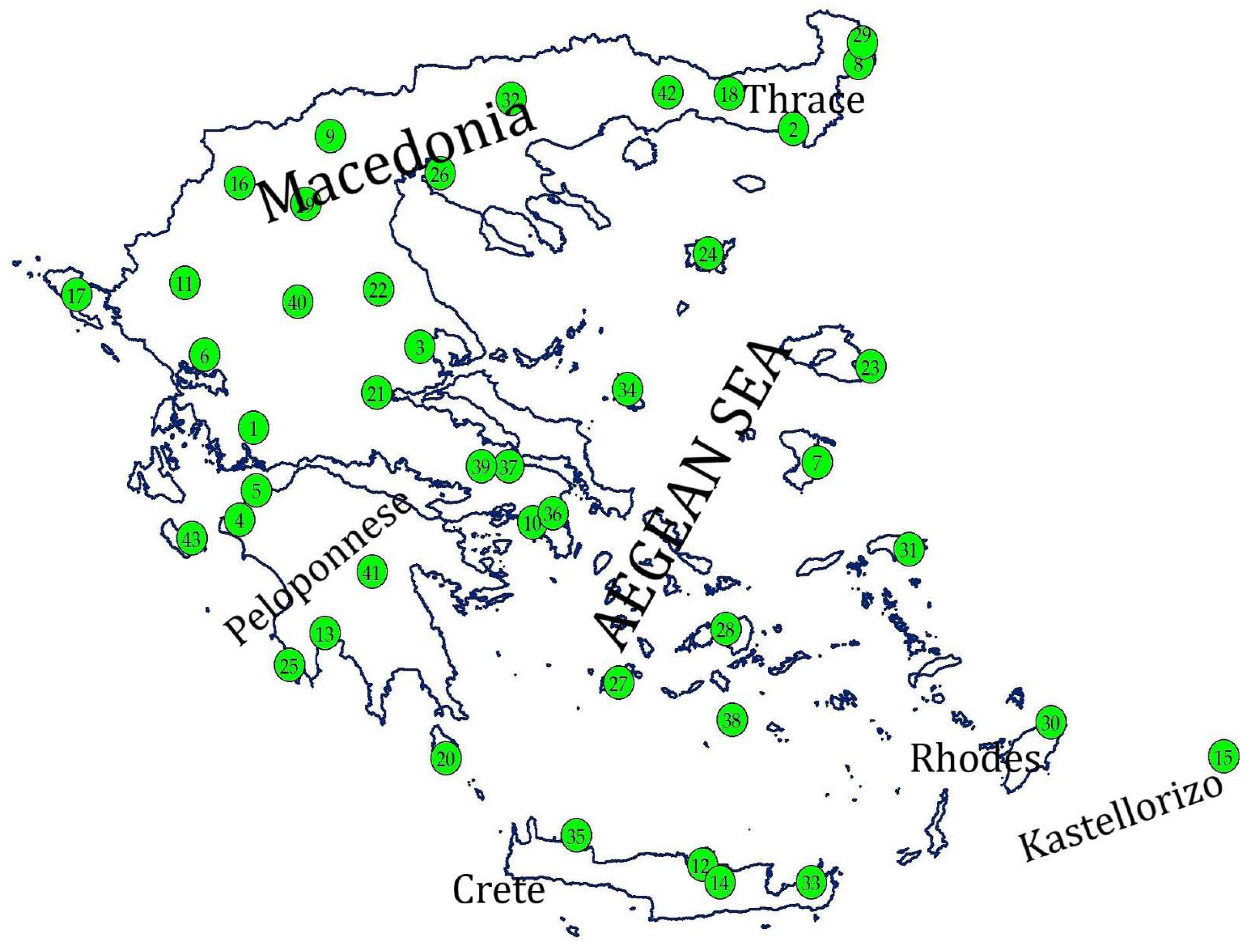
In the present work, a group of 43 sites was formed, which were arbitrarily chosen to cover the entire territory of Greece. The location of these sites was adopted from a recent study on the solar radiation climate of Greece [14]. Table 1 shows the names and geographical coordinates of the sites, while Figure 1 depicts their locations on a map of Greece.
TMYs for the above sites were obtained using the PVGIS tool; these TMYs include hourly values of: (a) air temperature (in degrees C); (b) relative humidity (in %); (c) horizontal infra-red irradiance (in Wm−2); (d) wind speed (in ms−1) and wind direction (in degrees); (e) surface barometric pressure (in Pa); (f) global horizontal solar irradiance, Hg (in Wm−2); (g) direct normal solar irradiance, Hbn (in Wm−2); and (h) diffuse horizontal solar irradiance, Hd (in Wm−2). The latter three parameters were considered in this study. The TMYs derived in the PVGIS platform resulted from simulations for the period 2005–2016.
2.2. Data Processing and Analysis
The data of the solar radiation parameters in the TMYs of the 43 sites were processed as follows.
Step 1. The hourly data downloaded from the PVGIS platform were converted from the universal time coordinate (UTC) into the local standard time (LST = UTC + 2 h for Greece) system. It should be noted here that the PVGIS solar radiation values were given at UTC times differentiating among the 43 sites; this means that they were given at hh:48 or hh:09, with hh = any hour between 00 and 23.
Step 2. The solar azimuths and altitudes for all TMYs and sites were derived using the solar code SUNAE (introduced by Walraven [35]). However, additional modifications to SUNAE to include atmospheric refraction and right ascension effects [36,37] have resulted in the XRONOS code (XRONOS = TIME in Greek, X is pronounced CH). Therefore, XRONOS was run for all 43 sites by inputting their geographical coordinates; the outputs of the algorithm were the solar altitudes, γ, at all LST times calculated in step 1 within their TMY. Nevertheless, inconsistencies (gaps) in the solar azimuth angles, ψ, at both instances of sunrise and sunset were found during the calculations using the XRONOS code. This discrepancy was overcome by implementing a modified XRONOS (mXRONOS) code in MATLAB; a Fourier series approximation of the expression for ψ at the sunrise and sunset instances was derived and applied to all 43 sites. The mXRONOS algorithm is described in detail in an article recently published in the journal Sun and Geosphere [38].
Step 3. The hourly direct horizontal solar irradiance, Hb, values were further estimated at all sites using the expression Hb = Hbn·sin γ.
Step 4. All solar radiation and solar geometry values were allocated to the nearest LST hour; this means that values at hh:48 LST or hh:09 LST were characterized as hh:00 LST, meaning they were accommodated at integer hours.
Step 5. Hourly solar irradiance values ≥ 0 Wm−2 or those corresponding to γ ≥ 5° (to avoid the cosine effect) were excluded from further analysis. In addition, another quality-test criterion (Hd ≤ Hg) was set at the hourly level.
To estimate the global solar irradiance on a flat-plate solar collector mounted on a dual-axis solar tracker, Hg,t (in Wm−2), one isotropic (Liu-Jordan (L-J) [39]) and one anisotropic (Hay [40,41]) models were adopted (subscript t = tracking). These models were used to estimate (i) the ground-reflected radiation on the sloping solar panels from the surrounding terrain, Hr,t (in Wm−2), and (ii) the diffuse-inclined radiation, Hd,t (in Wm−2). These models were adopted in the present work because of their simplicity and effectiveness in providing the tilted total solar radiation; a second reason for using both transposition models was to compare their results. The satisfactory performance of the L-J and Hay models has been verified in relevant publications, e.g., [42,43].
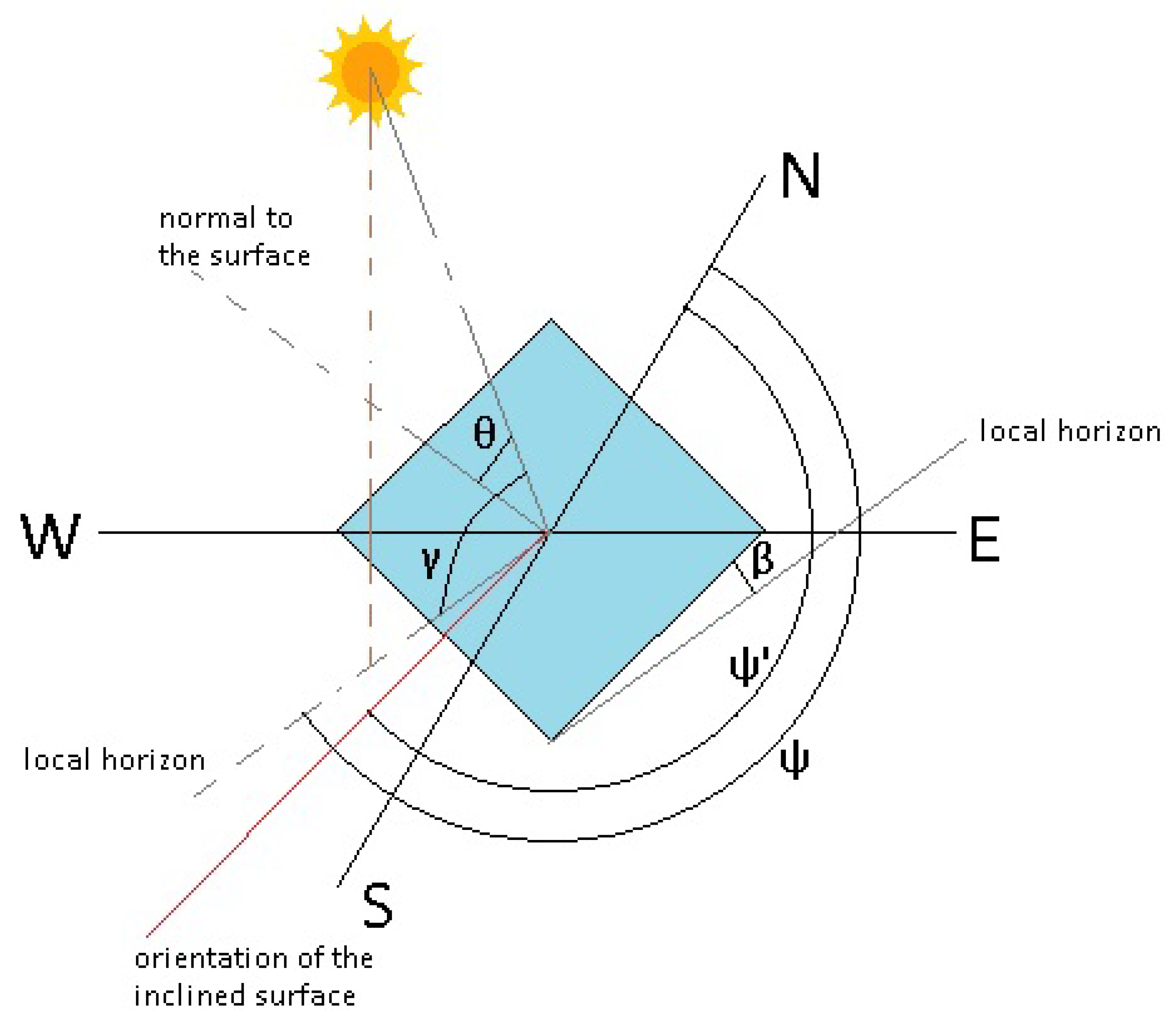
Figure 2 shows a schematic of solar rays incident on a tilted surface. The tilted surface was deliberately not aligned with the direction of the sun; this was done to show the various angles formed (the tilt angle of the inclined surface, β, the solar altitude, γ, the incidence angle, θ (the angle between the normal to the sloping surface and the direction toward the sun), the solar azimuth, ψ, and the azimuth of the sloping plane, ψ′.
For a surface mounted on a dual-axis solar tracker, the received global solar radiation is:
Hg,t = Hb,t + Hd,t + Hr,t,
The solar radiation components in Equation (1) are calculated by the following analytical expressions:
where, in this case, θ = 0° and β = 90° − γ (the sloping surface is always normal to the direct solar rays, see Figure 2); also, ψ = ψ′, because of the sun-tracking feature of the mode-III system. Rd = sky-configuration factor, Rr = ground-inclined plane-configuration factor, S = sun–earth distance correction factor, and N = day number of the year (N = 1 for January 1, and N = 365 for December 31 in a non-leap year or N = 366 in a leap year). The L-J model usually considers a ground albedo of ρg0 equal to 0.2 (see Equation (2)). Nevertheless, in the present study, ρg0 was replaced with the near-real ground albedo value, ρg, for all 43 sites. Therefore, monthly mean ρg values for the 43 sites were retrieved from the Giovanni portal [44] for pixels centered over each of the 43 sites (0.5° × 0.625°spatial resolution) during 2005–2016. These ρg values were subsequently used to calculate Hg,t at all the sites.
Hr,t = Hg·Rr·ρg,
Rr = (1 − cosβ)/2 = (1 − sinγ)/2,
Hd,t = Hd·Rd,model, (model = L-J or HAY),
Rd,L-J = (1 + cosβ)/2 = (1 + sinγ)/2,
Rd,Hay = Kb·Rb + (1 − Kb) ·Rd,L-J,
Rb = max(cosθ/sinγ,0),
Kb = min(Hb/Hex,1),
Hb,t = Hb·cosθ/sinγ = Hb·cos0/sinβ = Hb/cosγ,
cosθ = sinβ·cosγ·cos(ψ − ψ′) + cosβ·sinγ,
Hex = H0·S·sinγ,
H0 = 1361.1 Wm−2 (recent solar constant),
S = 1 + 0.033·cos(2·π·N/365),
Hb,t = Hb·cosθ/sinγ = Hb·cos0/sinβ = Hb/cosγ,
To isolate the solar radiation values that corresponded to clear-sky conditions only, the modified clearness index, k′t, was used, as in [45]. The significance of this modified index is that it does not depend on air mass [46]. Its definition is as follows:
where m is the optical air mass. Kambezidis and Psiloglou [45] defined the range of clear skies as 0.65 < k′t ≤ 1. This range was used in the present study, whereas the all-sky conditions were characterized by the full range of 0 < k′t ≤ 1. The atmospheric extinction index, ke, was adopted from [47] and is defined as ke = Hd/Hb [48]. This means that it provides information about the percentage (%) contribution of both Hd and Hb components to solar applications over a site, particularly to PV installations. In other words, it shows the significance of the fractional contribution of each solar radiation component to solar harvesting.
k′t = kt/{0.1 + 1.031· exp[−1.4/(0.9 + (9.4/m))]},
m = 1/[sinγ + 0.50572 · (γ + 6.07995)−1.6364],
kt = Hg/S · H0 · sinγ,
Equations (1)–(3), (4a), (5) and (10) are after [49]; Equation (4b) is according to [39]; Equations (4c)–(4e) follow [40,41]; Equations (6) and (7) are after [50]; Equation (8) is after [51], Equation (9) is after [52], and Equation (12) is according to [53].
For every site, Equation (1) was applied twice to estimate the hourly values of Hg,t; the first time by using Equations (4a) and (4b) for the L-J model and the second time by using Equations (4a)–(4e) for the Hay model. Annual/seasonal/monthly solar energy sums (in kWhm−2) under all- and clear-sky conditions were then calculated for all sites from the hourly Hg,t values. To implement all the above calculations, another MATLAB code was developed, which included the routine mXRONOS.
3. Results
3.1. Annual Solar Energy Potential
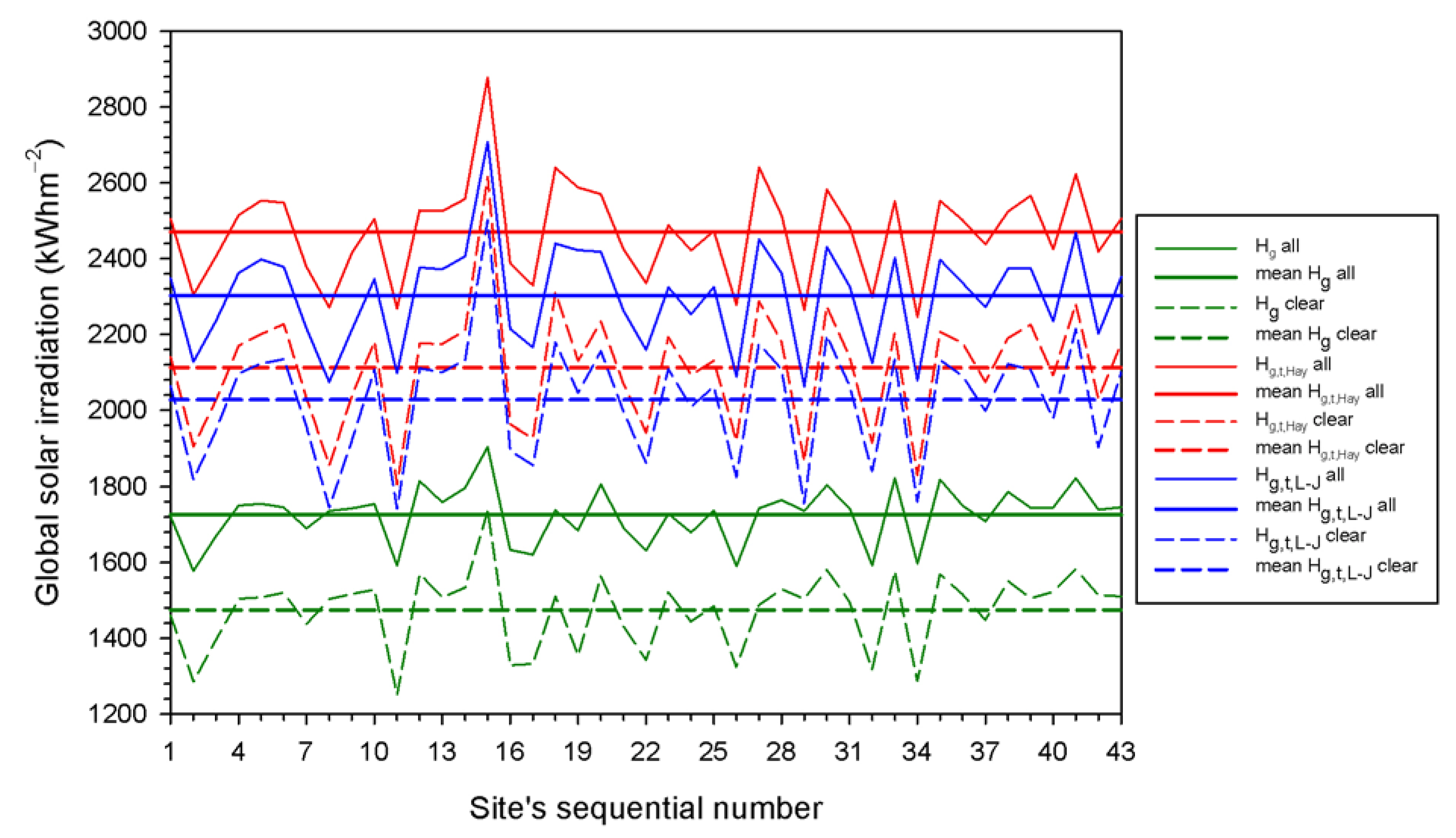
The annual solar energy sums were calculated from the database of each site using Equation (2) with ρg. By summing all hourly solar radiation values within the TMY for each site, the annual solar energy sum was derived for that location. The variation in the annual mean solar energy sums on horizontal and inclined flat-plate collectors mounted on mode-III solar trackers at the 43 sites in the examined period is depicted in Figure 3, and the diffuse solar radiation irradiation was estimated using both the transposition models of L-J and Hay. The difference in the average global solar irradiation value for the mode-III system compared to that on a horizontal surface is as follows: (i) the L-J model ≈572 kWhm−2 (or ≈33% increase) for all skies and ≈549 kWhm−2 (or ≈37% increase) in clear-sky conditions, and (ii) with the Hay model ≈745 kWhm−2 (or ≈43% increase) for all skies and ≈638 kWhm−2 (or ≈43% increase) under clear-sky conditions. The above results show that the Hay model estimates higher global inclined irradiation in all cases of weather conditions compared to the L-J model. Nevertheless, real solar radiation measurements on mode-III-configuration solar trackers do not officially exist in Greece, which means that the simulated results of the present study cannot be compared with real measurements. At first instance, these high differences indicate a preference for using mode-III solar systems instead of just horizontal solar collectors; this outcome would, however, be expected.
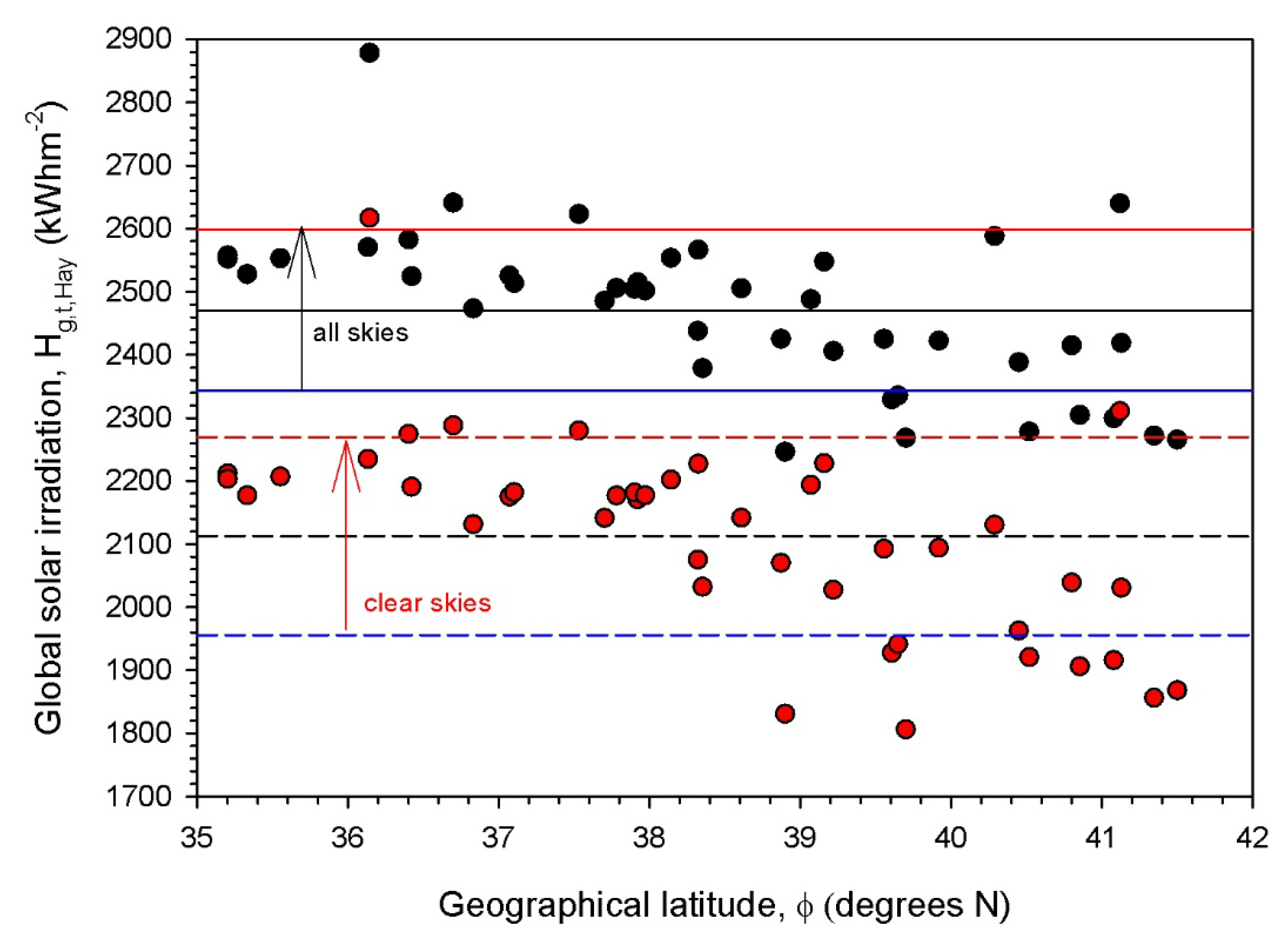
From Figure 3, one can see that Hg,t,L-J varies between 2064 kWhm−2 and 2709 kWhm−2 [(average) 2298 kWhm−2 ± (1σ) 133 kWhm−2 = 2165 kWhm−2 to 2431 kWhm−2] for all skies and between 1743 kWhm−2 and 2502 kWhm−2 [(average) 2023 kWhm−2 ± (1σ) 154 kWhm−2 = 1869 kWhm−2 to 2177 kWhm−2] for clear skies (σ = standard deviation); these values become for Hg,t,Hay 2247 kWhm−2 to 2878 kWhm−2 [(average) 2471 kWhm−2 ± (1σ) 127 kWhm−2 = 2344 kWhm−2 to 2598 kWhm−2, all skies] and 1806 kWhm−2 to 2617 kWhm−2 [(average) 2113 kWhm−2 ± (1σ) 156 kWhm−2 = 1956 kWhm−2 to 2269 kWhm−2, clear skies]. Figure 4 shows the above Hay-modeled findings in diagrammatic form. It can be seen that the standard-deviation band is narrower under all skies rather than clear ones, that is, higher dispersion of the clear-sky Hg,t,Hay values than the all-sky ones exists. This may be attributed to the selection process of the Hg,t,Hay values that fall in the clear-sky zone (i.e., 0.65 < k′t ≤ 1, Equation (11)); any criterion such as k′t cannot ensure 100% accuracy that the selected values of the variable will fully obey the criterion, but there may be other values of the variable that will falsely be classified in the clear-sky zone. Another observation from the graph in Figure 4 is that the solar irradiation values that lie outside the ±1σ band occur at higher latitudes, that is, for φ > 39° N. This finding may be attributed to the higher weather variability in the northern part of Greece than in the southern part, particularly under clear skies. More specifically, under all-sky conditions, seven (or 16.3%) Hg,t,Hay data points lie outside the ±1σ band for φ < 39° N and 8 (18.6%) for φ > 39° N, while under clear-sky conditions, only four (9.3%) Hg,t,Hay data points lie outside the ±1σ band for φ < 39° N and 9 (20.9%) for φ > 39° N.
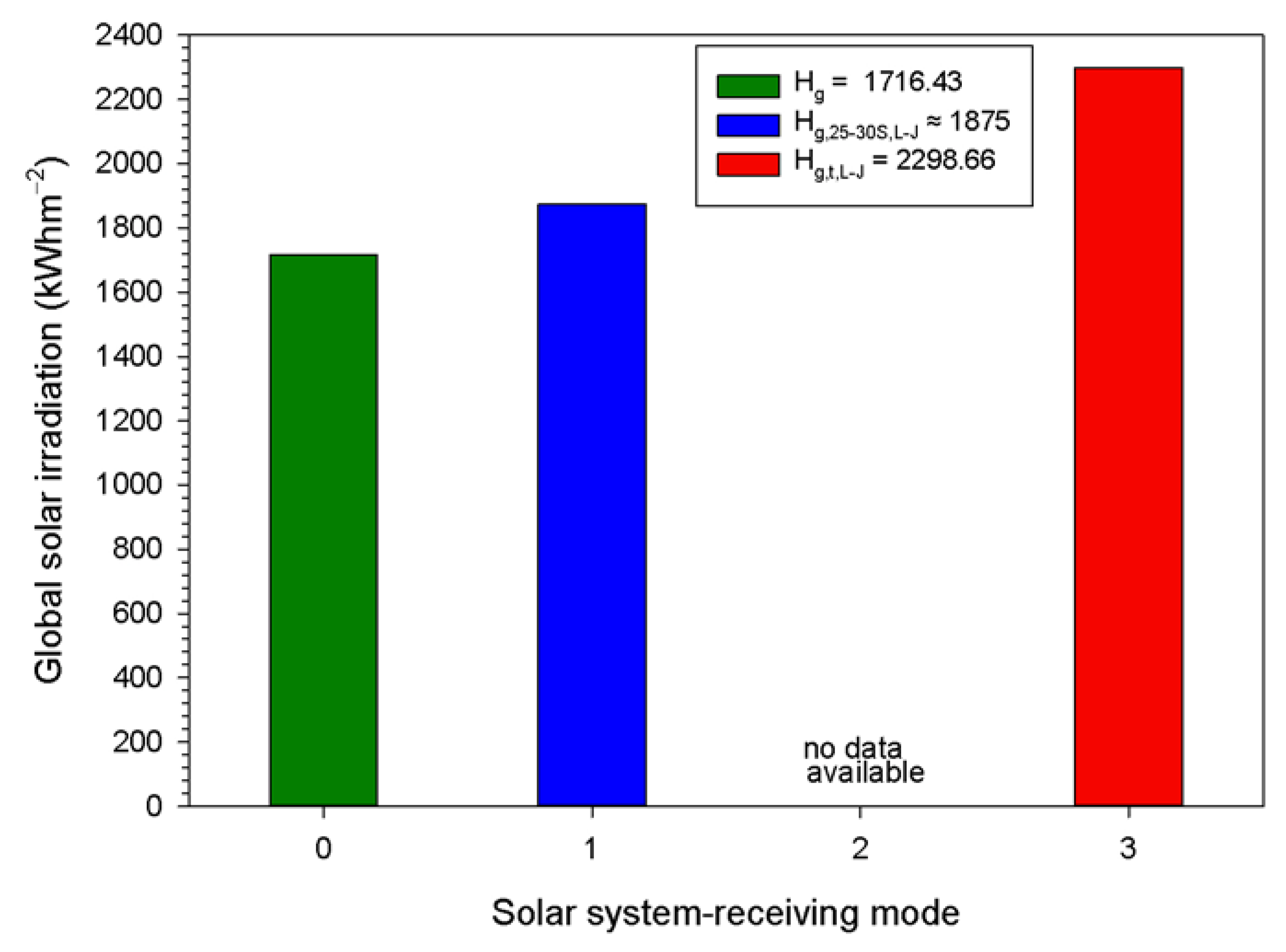
On the other hand, Kambezidis and Psiloglou [1], in their study on the solar energy efficiency of mode-I systems in Greece, did not report an annual average global solar irradiation value; nevertheless, this average was extracted from their Figure 6 resulting in ≈1875 kWhm−2 under all-sky conditions (the authors used the L-J model with ρg0 only). This gives a 9.23% increase with reference to the horizontal case and a 22.59% deficit in relation to mode-III systems (present study with L-J model and ρg). It is worth mentioning here that the above work was based on TMY data from 33 sites in Greece; the locations of the sites in that work coincide with the corresponding ones in the present 43-site study. For compatibility reasons, the locations of those 33 sites are considered in the calculations of this issue. To make the results more documentary, Figure 5 shows the superiority of mode-III solar systems in terms of solar-energy harvesting. Now, the differences between the modes are Hg,t,L-J/ρg − Hg,25-30S,L-J/ρg0 = 423.66 kWhm−2, Hg,t,L-J/ρg − Hg = 582.23 kWhm−2, and Hg,25-30S,L-J/ρg0 − Hg = 158.57 kWhm−2. As discussed in Section 3.3, any of these three differences are comparable to or even double the monthly mean global solar irradiation for a mode-III tracker across all 43 sites in Greece for all-sky conditions. This outcome gives another credit to investing in type-III solar trackers because an extra month or two is gained if maintenance costs are excluded. Farahat et al. [54] compared the three modes of solar harvesting in Saudi Arabia. They concluded that the Hay model should be preferred to the L-J model if a mode-III tracking system is used for solar energy capture. Therefore, the rest of the calculations and analyses in the present work were conducted with the Hay model alone.
Working with the Hay transposition model and near-real albedo values for the 33 sites in Greece, the annual solar energy potential on flat-plate solar collectors mounted on a dual-axis system was estimated at Hg,t,Hay/ρg = 83,440 kWhm−2 ± 108.19 kWhm−2 (all skies). For the 25°–30°-tilt, flat-plate solar collectors toward the south (1875 kWhm−2 per site × 33 sites), Hg,25-30S,L-J/ρg0 = 61,875 kWhm−2. The ratio of Hg,t,Hay/ρg over Hg,25-30S,L-J/ρg0 is 1.3485, which shows that the dual-axis system is ≈34.9% more efficient than the fixed-tilt system in Greece.
Table 2 shows the total annual solar energy yield per site for flat-plate solar collectors fixed on a two-axis solar tracker under all- and clear-sky conditions in Greece.
3.2. Monthly Solar Energy Potential
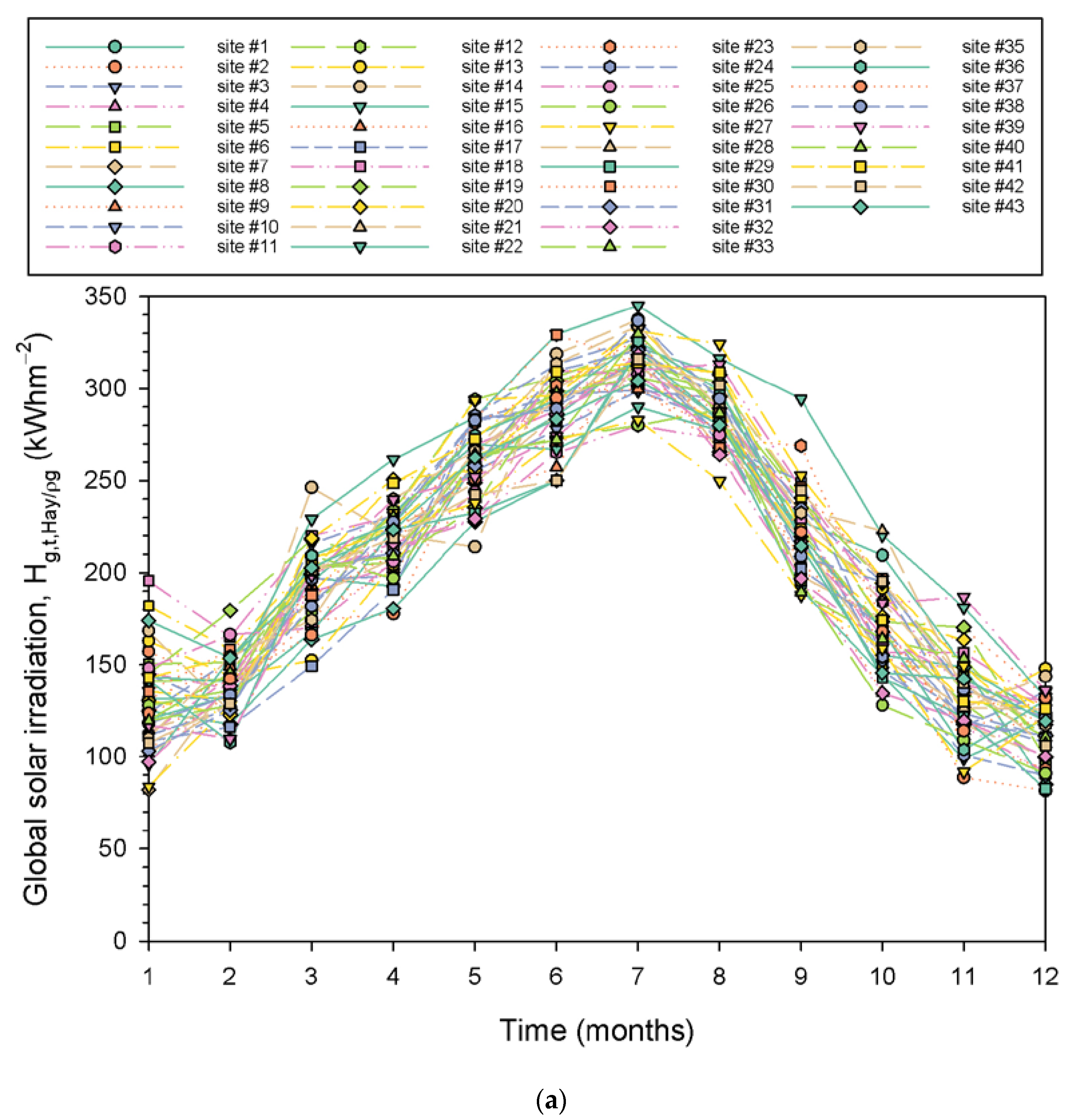
The intra-annual variations in Hg,t,Hay/ρg for the 43 sites are shown in Figure 6, The curves for almost all sites are remarkably close to each other, creating a bundle (zone) under all- (Figure 6a) and clear- (Figure 6b) sky conditions. The amplitude of this band (i.e., dispersion of the monthly mean values) is ≈150 Wm−2 in both cases. This can be confirmed by the comparable standard deviations in the average Hg,t,Hay/ρg values for all- (127 Wm−2) and clear- (157 Wm−2) sky conditions (third line from bottom in Table 2).
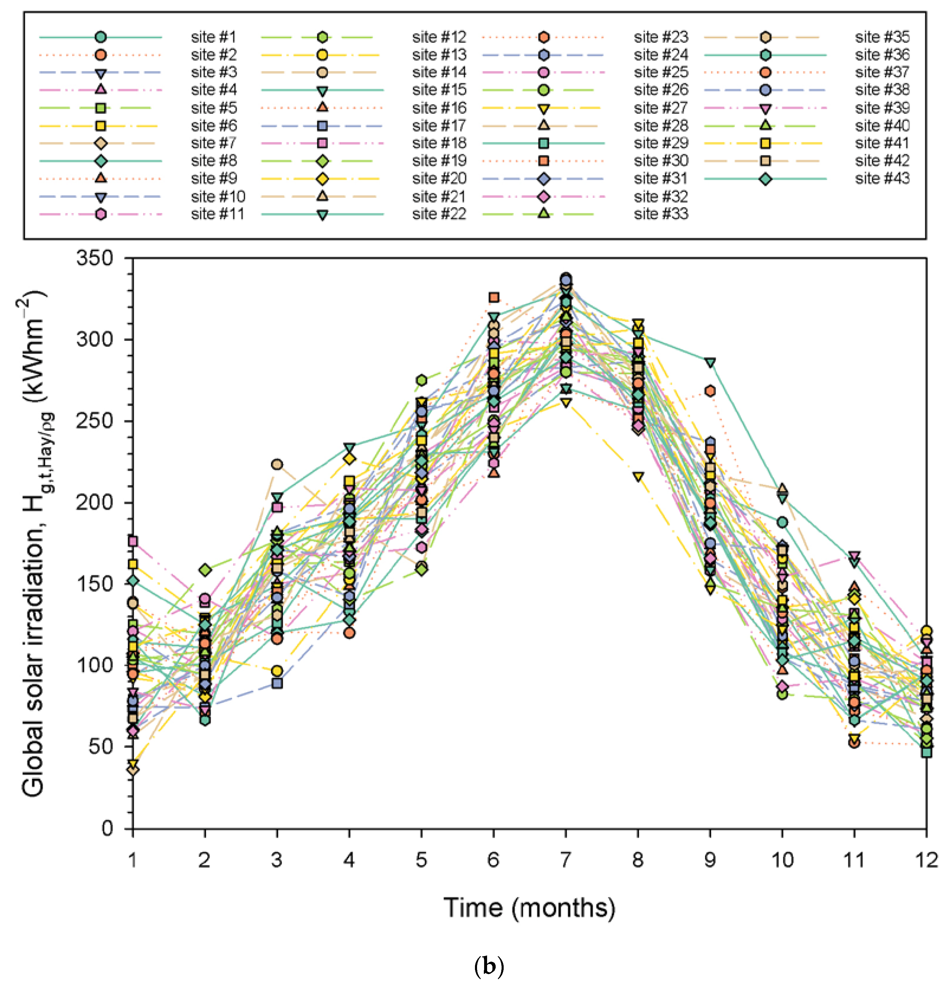
From Figure 6, information about the solar energy sum per site and month can be extracted. Nevertheless, this visual task may not be satisfactory for solar energy engineers and investors/entrepreneurs because they would be happy to have a guide that would provide them with a more precise estimate of the monthly solar energy. In this context, the monthly energy yields averaged over all sites and in their TMYs were estimated; Figure 7 shows their average intra-annual variation for all of Greece. The graphs also show the ±1σ curves around the mean curves and the polynomial curves that fit the mean curves. It is easy to see that both mean and polynomial fit curves lie within the ±1σ band; this implies that there are no abnormal (outliers) monthly values that would result in drifting of the mean and/or the fitted lines outside the ±1σ bands in all or certain months. Moreover, the peak Hg,t,Hay/ρg values occurred in July (Figure 6 and Figure 7), as anticipated. This is because Greece is a country not close to the equator; on the contrary, countries closer to the equator provide a different intra-annual solar energy potential with higher values in spring and autumn than in summer, for example [55], which is due to solar paths (solar analemmas [56,57]) over such locations year-round. Figure 7 shows the curves that best fit the mean ones in the form of sixth-order polynomials; their regression expressions are shown in Table 3. This order of polynomials was selected to provide the highest R2.
3.3. Seasonal Solar Energy Potential
In the Northern Hemisphere, the minimum and maximum energies received by solar receiving systems occur during winter and summer, respectively. Therefore, this section is dedicated to analyzing the seasonal solar energy availability during springtime (months of March–April–May), summertime (June–July–August), autumn (September–October–November), and winter (December–January–February). By summing all hourly solar radiation values in a season, the corresponding solar energy at each site can be calculated, and by averaging the seasonal solar energy values across the 43 sites, the seasonal mean energy is received.
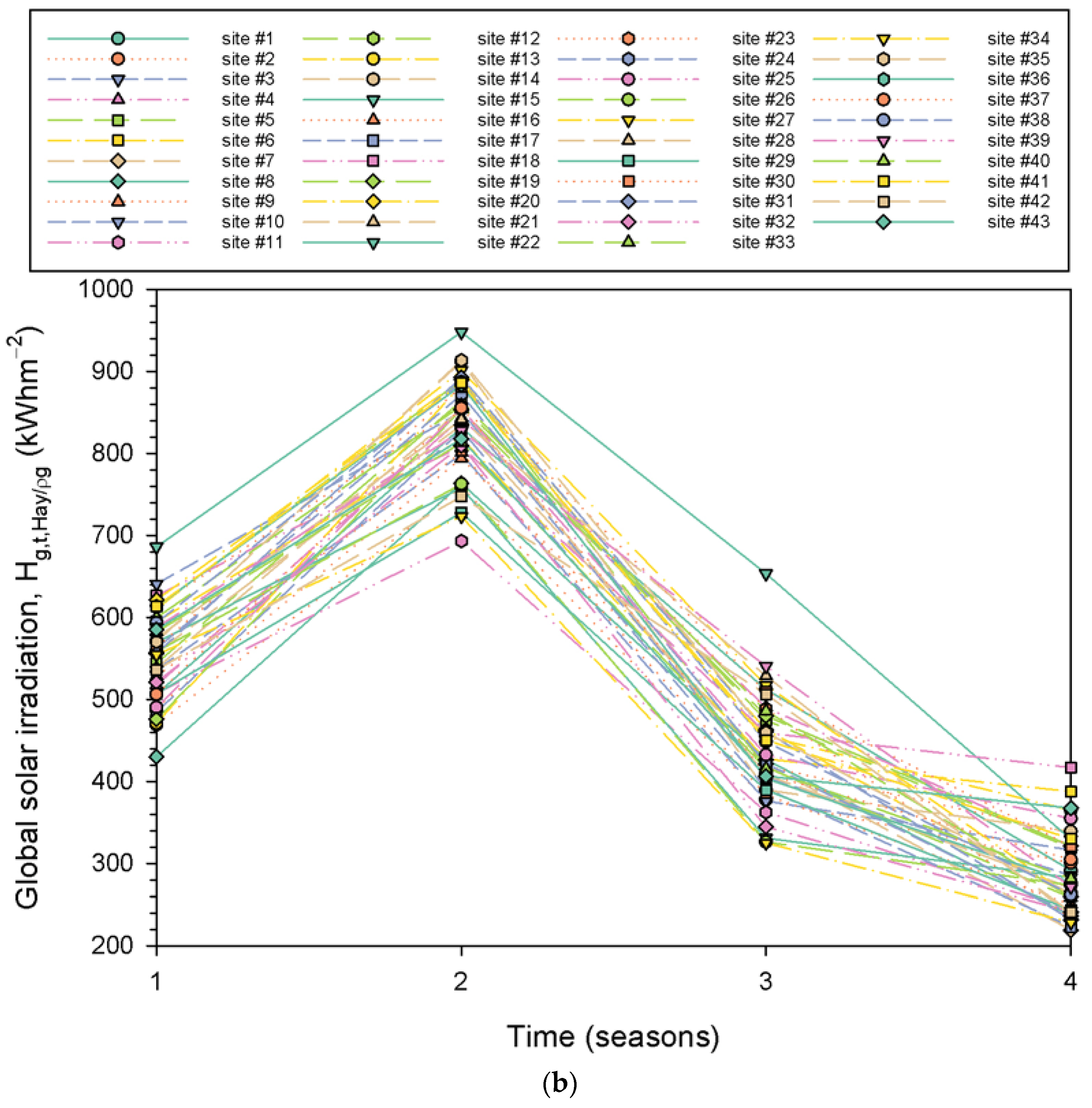
Similar to the presentation of the intra-annual (i.e., monthly) variation in the Hg,t,Hay/ρg levels (cf. Figure 6), Figure 8 presents the seasonal solar energy potential across all sites in Greece. As expected, the solar energy potential peaks during summer for all sites. Exceptionally higher Hg,t,Hay/ρg levels occur at the Kastellorizo site (site #15 on the map of Greece in Figure 1, a site at the southeastern corner of the country). The high annual solar energy potential of Kastellorizo is depicted in Figure 4 (black and red dots at φ = 36.14° N), and in Table 2 (site #15).
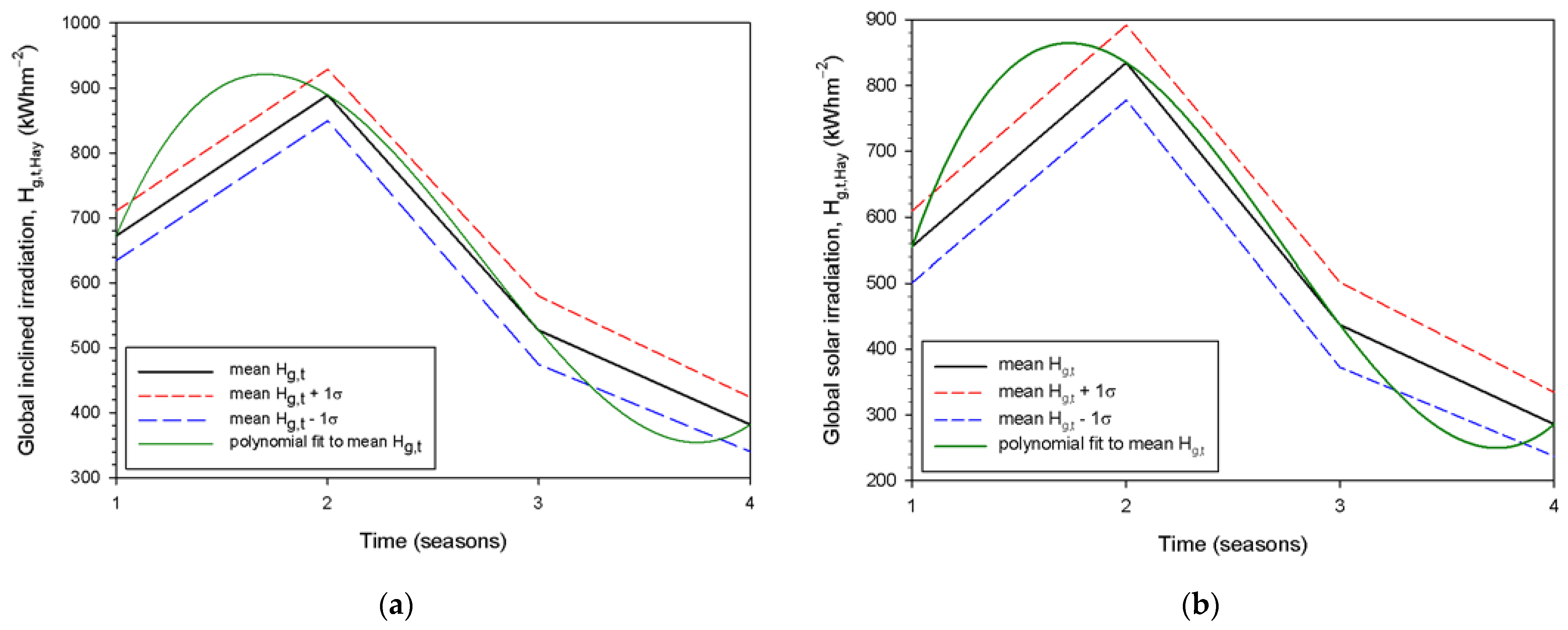
To derive a single expression for the average seasonal energy yield in Greece, the energy values for the same season from all sites were averaged over their TMYs but separately under all- and clear-sky conditions; the results are presented in Figure 9. Table 3 provides the non-linear regression equations for the curves that best fit the seasonal mean solar energy values. It should be noted that all fits are ideal (R2 = 1).
3.4. Maps of Annual Solar Energy Potential
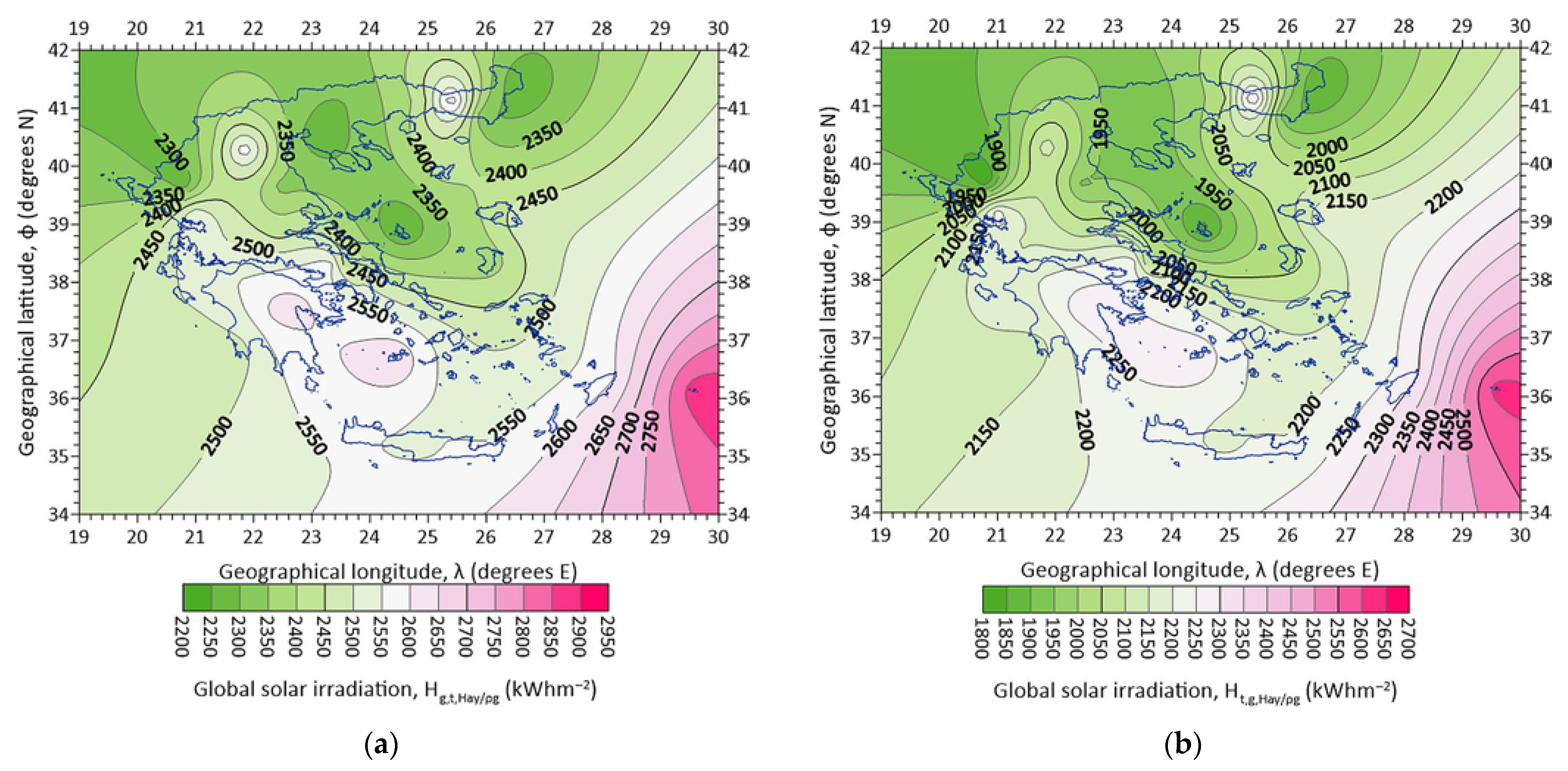
Figure 10 shows the solar energy potential over Greece with respect to the annual Hg,t,Hay/ρg yields. A gradual increase is observed in the annual solar energy potential in the direction N-S for both all- (Figure 10a) and clear- (Figure 10b) sky conditions. Such a trend was found for the solar horizontal irradiances in Greece (see Figure 10b in [14]), as well as for the solar radiation received on flat-plate collectors tilted to the south at 25°–30° (see Figure 11a in [1]). From Figure 10a,b of the present work, one can easily realize that, in both cases, an (imaginary) horizontal line at φ ≈ 39° N divides the country into a northern part with lower solar energy availability and a southern one with higher Hg,t,Hay/ρg levels. This was confirmed by a study of the solar radiation climate of Greece [14], in which the dividing line was also placed at φ = 39° N. Amazingly, the Hg,t,Hay/ρg patterns in Figure 10a,b are almost identical. The remarkable similarity may be attributed to two factors. (i) Latitude: at higher latitudes, lower solar radiation levels are received by a horizontal plane on the surface of the earth and consequently on inclined flat-plate surfaces. (ii) Meteorology: more frequent cloudiness occurs in the northern part of the country; indeed, a relevant study for the cloudiness over the Mediterranean region shows a similar pattern over Greece on an annual basis to that in our Figure 10a (cf. Figure 1i in [58]).
3.5. Specialized Analysis
This section focuses on specific issues that were not included in the previous analysis. The topics to be addressed are as follows: (i) accuracy of the PVGIS simulations and variation in Hg,t,Hay/ρg versus Hg,t,L-J/ρg for all- and clear-sky conditions; (ii) effect of the ke index on solar harvesting (i.e., Hg,t,Hay/ρg); (iii) seasonal and monthly variation in ke; (iv) dependence of the annual Hg,t,Hay/ρg values on φ, z, or ρg; (v) seasonal maps of Hg,t,Hay/ρg; (vi) 3D maps of the annual Hg,t,Hay/ρg values versus φ and ρg; and (vii) intra-annual variation in ρg. All these are examined under all-sky conditions, except for (i).
- (i)
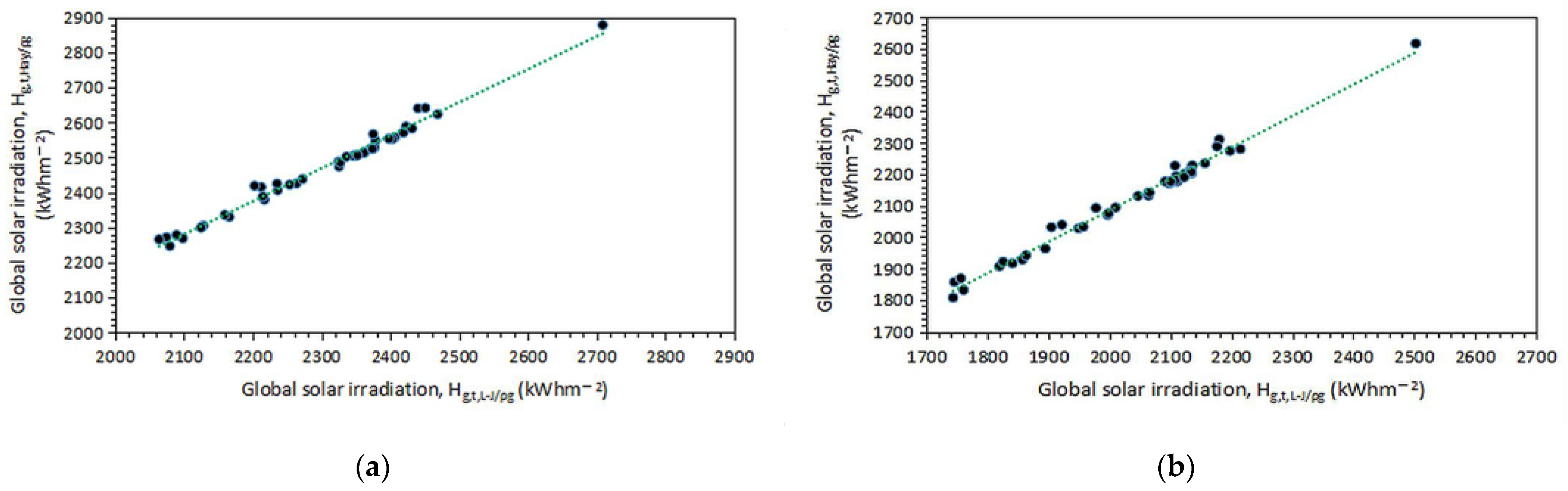
- Various researchers [33,34,59,60] have shown that the PVGIS tool simulates values for a solar horizontal radiation with an accuracy between −14% and +11% (a median value of −1.5% is, therefore, very comparable to the ±3% accuracy of most pyranometers). This was done by comparing the PVGIS-simulated solar radiation values with real measurements. Thus, no new evaluation was required for the PVGIS tool. As far as the interdependence of the Hg,t,Hay/ρg- and Hg,t,L-J/ρg-estimated values is concerned, this is shown in Figure 11a for all- and Figure 11b for clear-sky conditions. In both cases, the interdependence is linear, as anticipated.
- (ii)
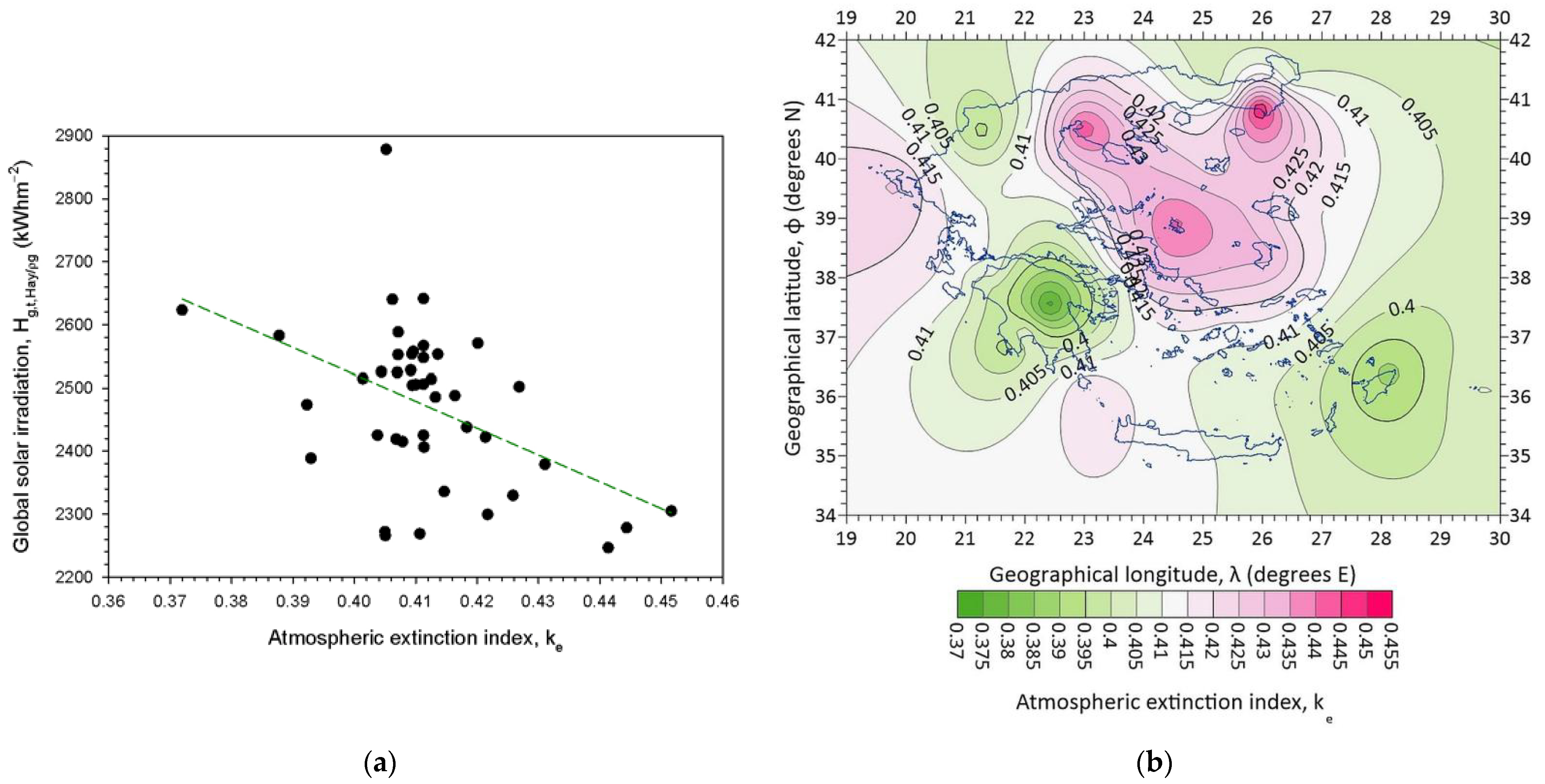
- Figure 12a shows the dependence of Hg,t,Hay/ρg on ke. A linear fit to the data points was derived with a negative slope, which implies decreasing solar irradiation values with an increasing atmospheric extinction index. In other words, a 0.1 increase in ke results in an almost 1273 kWhm−2 decrease in Hg,t,Hay/ρg (calculated by applying the linear expression in Figure 12a twice for ke1 = 0.38 and ke2 = 0.48, computing the Hg,t,Hay/ρg1 and Hg,t,Hay/ρg2 values, and taking their difference (Hg,t,Hay/ρg2 − Hg,t,Hay/ρg1). As these energy values concern the entire Greek territory (i.e., the average value for all 43 sites), then a decrease of about 30 kWhm−2 (=1273/43) per site in a year-round is calculated or a decrease of ≈2.5 kWhm−2 (=30/12) per site and per month. From Figure 7a, one sees that the average energy yield for January (worst case) is about 130 kWhm−2 for all 43 sites or about 3.0 kWhm−2 (=130/43) per site, and 330 kWhm−2 in July (best case) for all 43 sites or 7.8 kWhm−2 (=330/43) per site. The site-month values of 3.0 (or 7.8) kWhm−2 are comparable to (or 3 times higher than) the 2.5 kWhm−2 decrease in Hg,t,Hay/ρg due to a 0.1 increase in ke. Since ke = Hd/Hb (consider Hb = constant), a 0.1 increase in ke means a 10% increase in Hd and a subsequent decrease in Hg,t,Hay/ρg equal to 1273 kWhm−2 (or 14% equivalently). Therefore, any solar energy investor in Greece should consult not only the solar energy potential map of Greece (Figure 10a) but also the corresponding map of ke in Figure 12b. In the latter map, higher ke values occur over the northern Aegean Sea, Macedonia, and Thrace regions and lower ones over Peloponnese, Crete, and Rhodes. Considering that a constant Hb value indicates that favorable areas for solar harvesting in Greece are those of Peloponnese, Crete, and Rhodes because the contribution of the diffuse solar component is less important than in the northern areas, no extra cost in the solar panel material is anticipated to exploit the higher diffuse radiation in northern Greece with respect to the Hb component.
- (iii)
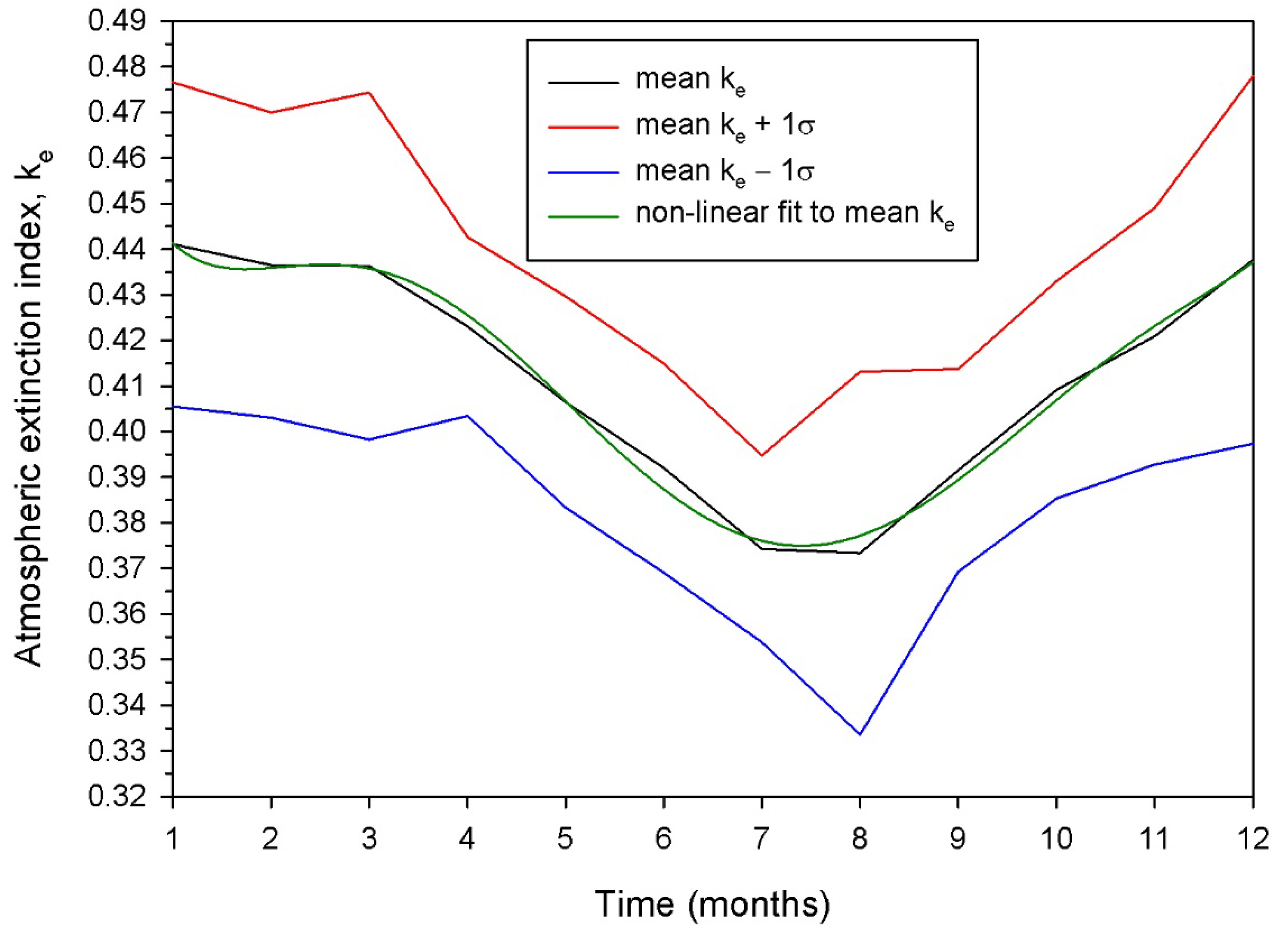
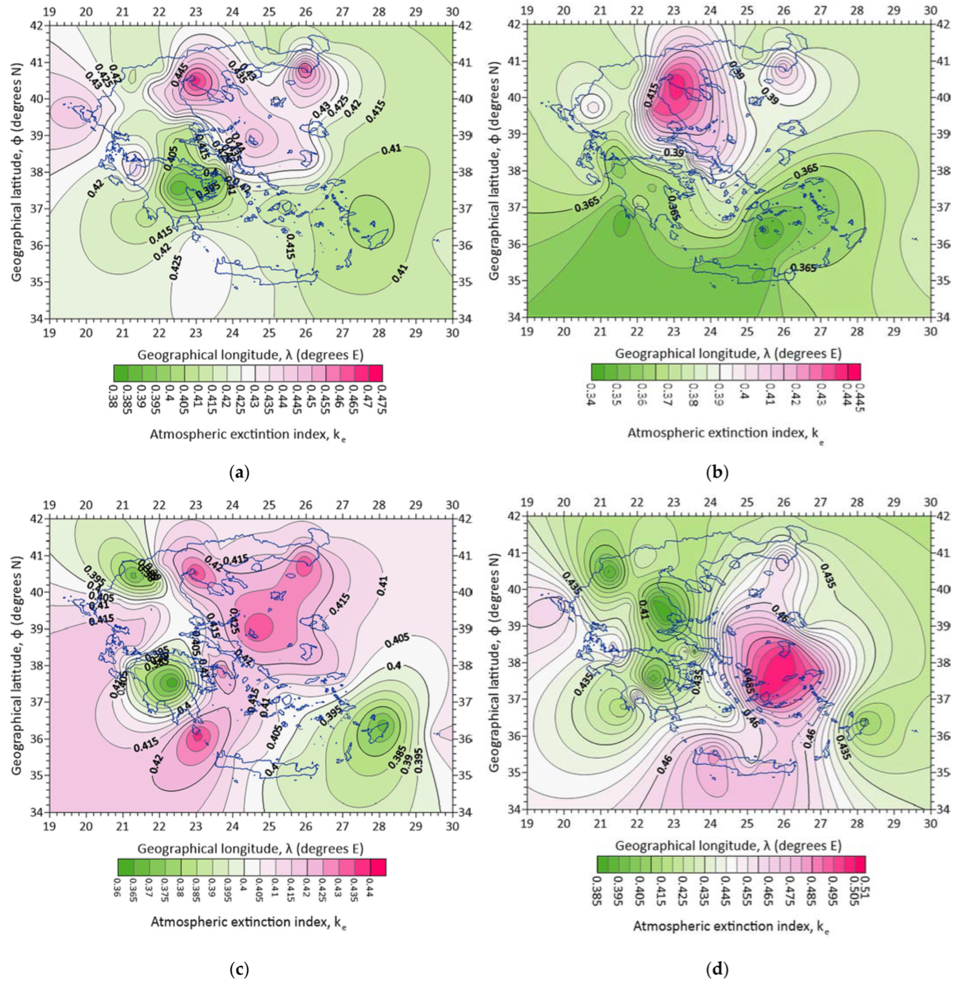
- Now that the importance of the ke index in solar harvesting has been established, it is useful to derive and present the monthly and seasonal mean variation in the index for Greece. Figure 13 shows the intra-annual variations in the ke. It is interesting to observe that minimum values occur in the summertime due to lower Hd/Hb values; this is also because, on the one hand, the Hd levels are lower than in the other seasons (less frequent cloudiness), and, on the other hand, the Hb levels are higher in this season. The above observations are also confirmed by Figure 14, which presents the seasonal variation in ke under all-sky conditions in Greece. The spring and summer ke patterns are remarkably similar, with higher values in the northern part of Greece and lower values in the south. The lower ke values imply lower diffuse radiation in comparison to the direct one; therefore, solar panels need to exploit the direct solar component without paying attention to the diffuse component in southern Greece. In contrast, diffuse radiation becomes more dominant in northern Greece, and this must be considered in PV installations. This outcome indicates a preference for solar harvesting below the latitude of φ ≈ 39° N (same conclusion in Section 3.4 for the annual values of Hg,t,Hay/ρg) during spring and summer. In contrast, the autumn and winter patterns differ; some relatively high values are observed over the northern Aegean Sea, Macedonia, Thrace, and south of Peloponnese (autumn), Crete, and almost all of the Aegean Sea (winter). In these two seasons, the rule of an imaginary dividing line at φ ≈ 39° N is not obeyed.
- (iv)
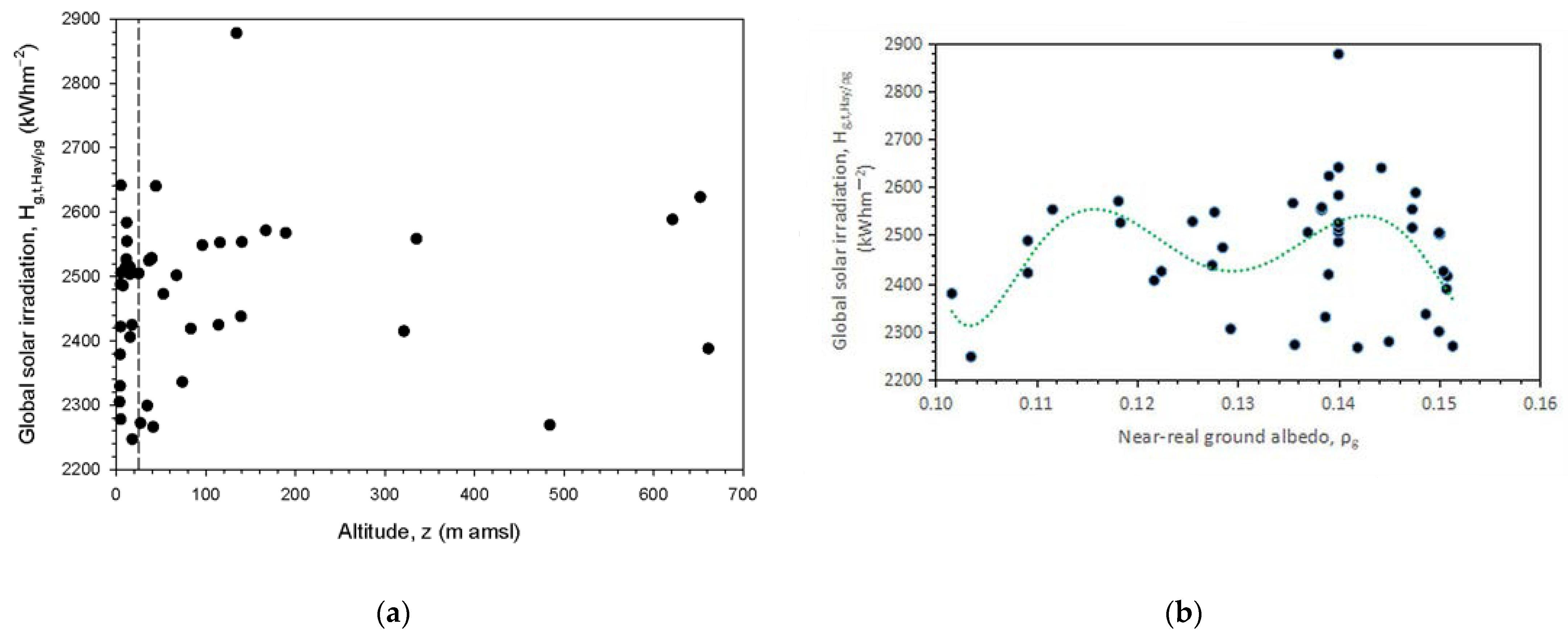
- The variations in the annual Hg,t,Hay/ρg values versus φ were presented in Figure 4. Here, analogous plots were derived with respect to z and ρg. The variation in the annual Hg,t,Hay/ρg values versus z is shown in Figure 15a, while the variation in Hg,t,Hay/ρg versus ρg is shown in Figure 15b. In both figures, a wide dispersion of the Hg,t,Hay values versus z or ρg is observed; moreover, many Hg,t,Hay values occur at lower elevations (below 25 m amsl, vertical dashed line in Figure 15a), which shows that the global solar irradiation is not strictly related to the altitude of the site (at least in the range of 0–700 m amsl). Indeed, 16 of 43 sites (37.2%) are at altitudes lower than 25 m amsl. A similar conclusion is drawn from Figure 15b; here, the sixth-order polynomial fit is shown to form two peaks at ρg ≈ 0.116 and ≈ 0.144. The very loose dependence of solar irradiation (for flat-plate solar panels fixed on dual-axis systems in Greece) either on the site location (i.e., geographical latitude) or the type of ground (i.e., ground albedo) concludes that the general rule for solar energy system installation is only the region (northern or southern Greece, see Figure 10 and Figure 16).
- (v)
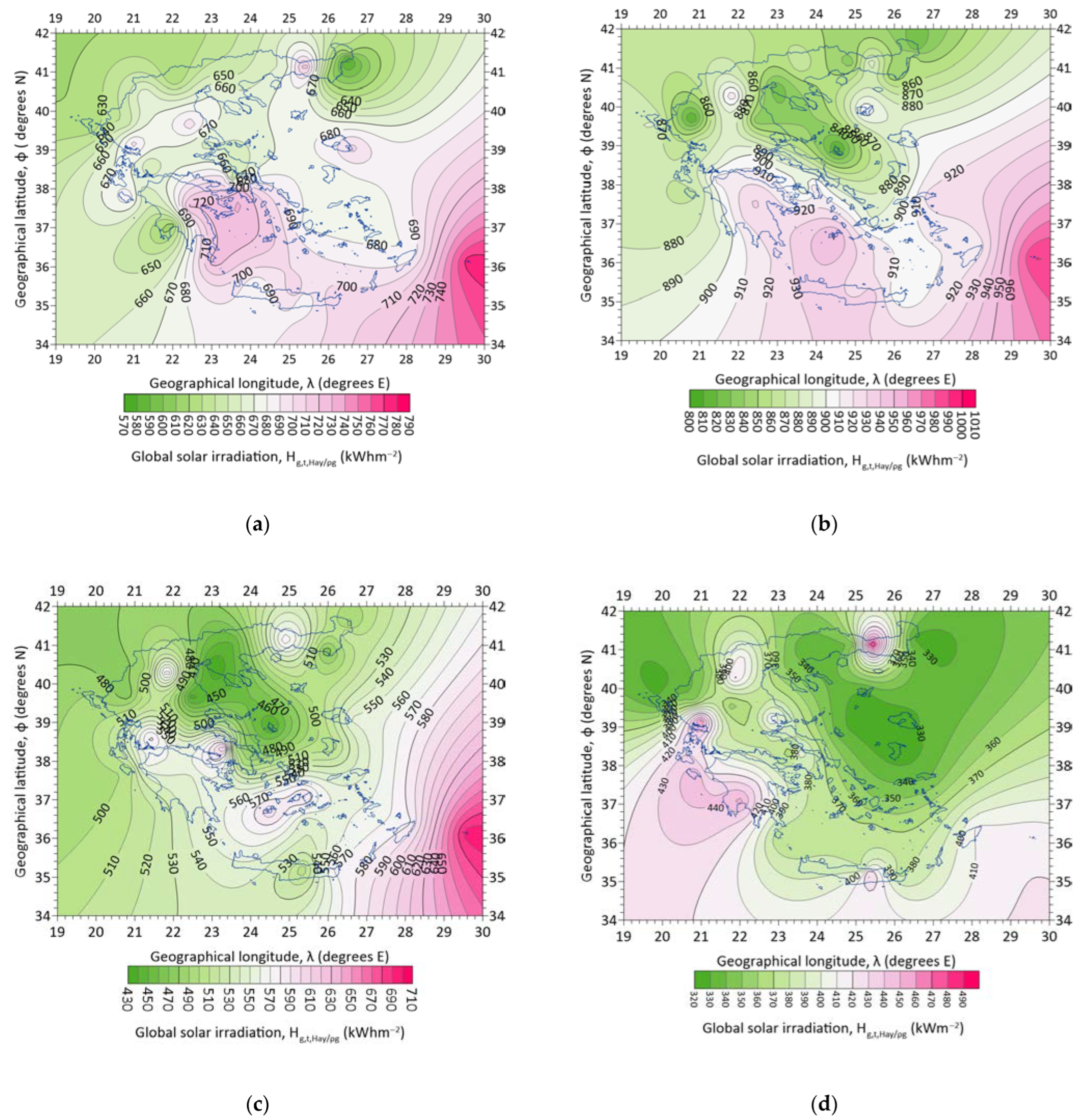
- Four seasonal maps of Hg,t,Hay/ρg over Greece under all-sky conditions are presented in Figure 16. The Hg,t,Hay/ρg patterns are the opposite of those for ke in the corresponding seasons. This is quite logical because high global solar radiation consists mainly of direct solar component and less of diffuse solar radiation; this is equivalent to low ke (i.e., Hd/Hb) values and vice versa.
- (vi)
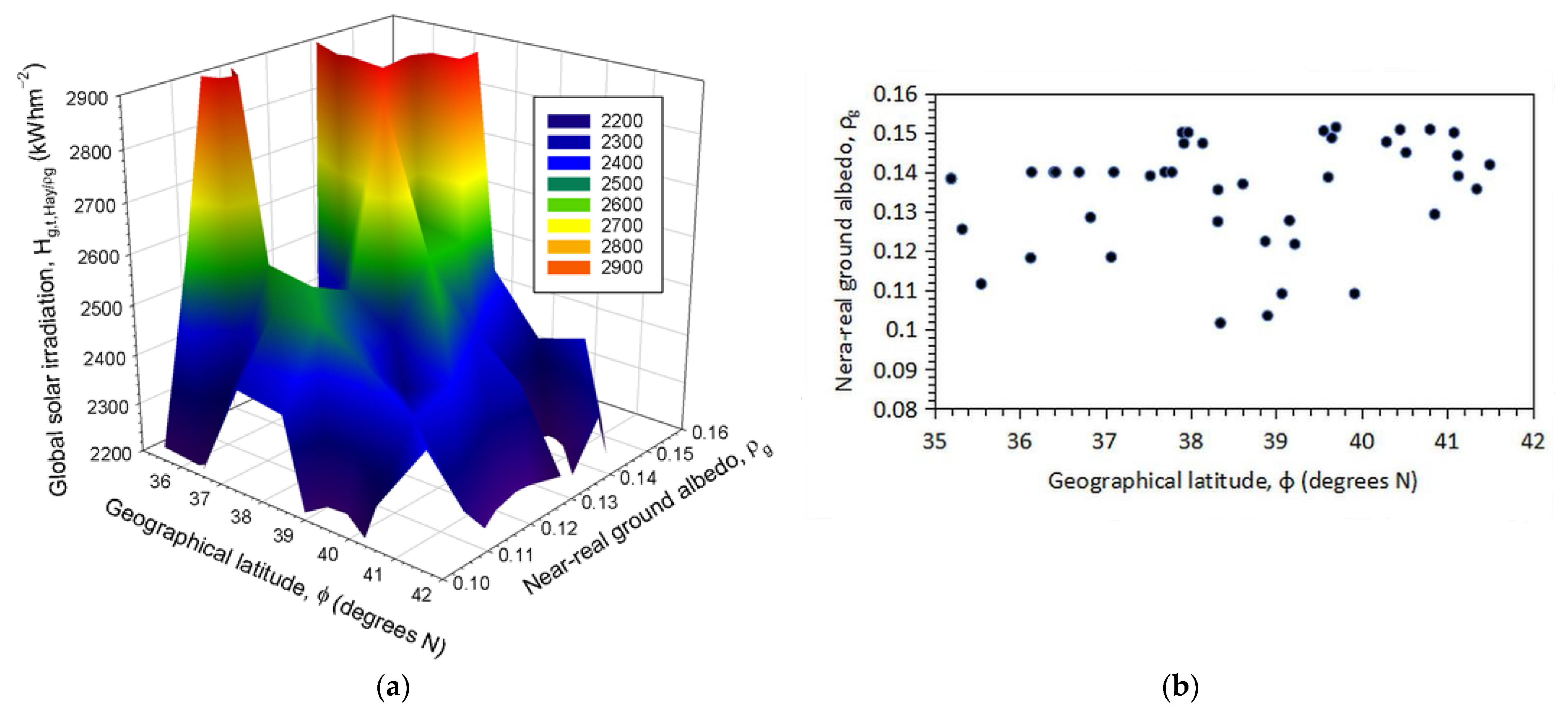
- A 3D graph of Hg,t,Hay/ρg versus φ is presented in Figure 17a, and a scatter plot of ρg versus φ in Figure 17b, both under all-sky conditions. The Hg,t,Hay/ρg pattern has a wave-like shape, as confirmed by the 2D plot, in which the green line is a sixth-order polynomial fit to the data points. This is an interesting result and shows that reflections from the ground play a role in the performance of a double-axis solar system. The large scatter in the data points of Figure 17b implies that the ground reflections do not depend directly on the geographical latitude; however, two peaks in the ρg values can be observed for φ ≈ 38° N and φ ≈ 41° N, which correspond to sites located in central and northern Greece, where green lands (forests or cultivated areas) exist that reflect more radiation than the bare soil in most parts of the southern territories of the country (for φ < 38° N). Apart from the general territory rule of φ ≈ 39° N (see Figure 10 and Figure 16) in investing solar energy systems in Greece formulated in (iv) above, one should also consider that a system installed at a site with φ = 38° N or φ = 41° N may receive almost 1.4 times higher ground reflection than other sites at φ ≈ 36° N or φ ≈ 39° N. However, a combination of Figure 15b and Figure 17b results in Figure 17a, in which the solar irradiation levels over Greece take a waveform pattern.
- (vii)
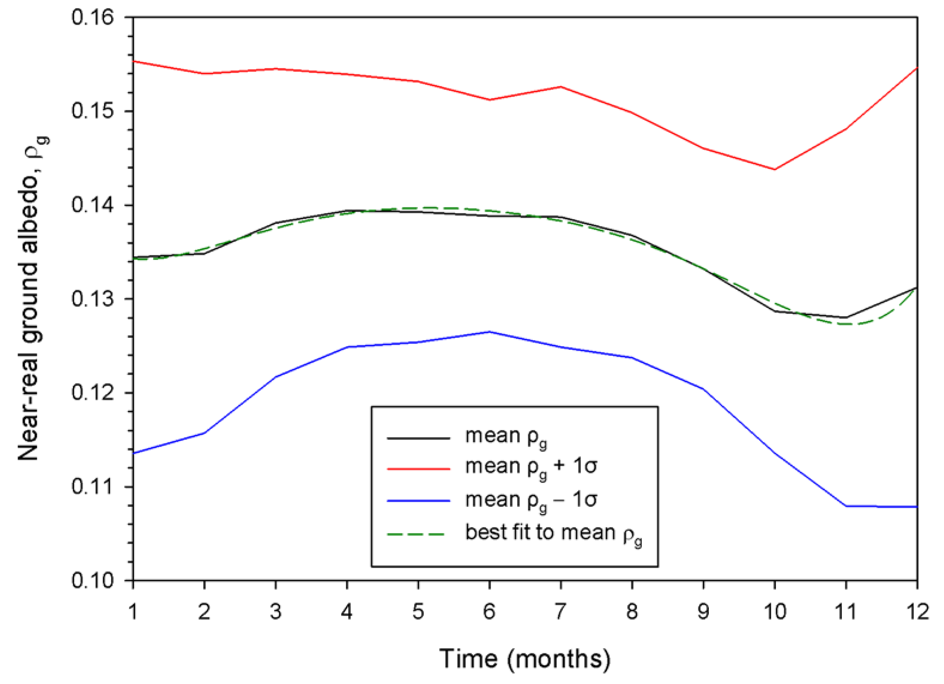
- Figure 18 presents the intra-annual (i.e., monthly) variation in the near-real ground albedo over Greece. The mean ρg ± 1σ band is also shown, which implies a ρg variation in the range of 0.108–0.155. This broad ±1σ band is justified by the wide dispersion of the annual ρg values in relation to φ shown in Figure 17b. Nevertheless, the annual mean ρg value for Greece was estimated to be 0.135. Psiloglou and Kambezidis [61] estimated an annual ground albedo value for Athens of 0.145 from solar radiation measurements performed at the Actinometric Station, National Observatory of Athens, Greece, in the period 1999–2008.
4. Discussion
This section discusses the results obtained by other researchers.
Hammad et al. [62] compared the performance and cost of static (fixed-tilt) and dynamic (two-axis) systems. They found that the dual-axis systems produced 31.29% more energy than the static ones, a figure quite comparable to our 34.85% (or 1.3485 times) increase found in Section 3.1. Further, the authors calculated the payback period and found it to be 27.6 months for dynamic and 34.9 months for static systems, with corresponding electricity costs of $0.080 kWh−1 and $0.100 kWh−1.
Lazaroiu et al. [63] found that a double-axis solar system produces 12–20% more energy than a fixed-tilt one in Romania, quite lower than our ≈35%.
In Saudi Arabia, Kambezidis et al. [64] found that mode-III systems produce 4.22% more solar energy than mode-II systems, 28.81% more solar energy than mode-I systems, and 37% more solar energy than a flat-plate receiving surface on horizontal plane. Their result of 28.81% is close to our value of 34.85%.
Drury et al. [65] showed that for mode-II tracking systems in the USA, the generated solar energy can increase by 12–25% in relation to fixed-tilt ones, while the operation of mode-III tracking systems increases by 30–45%; the latter finding includes our ≈35%. These researchers estimated the installation cost to be $0.25 W−1 for fixed-tilt, $0.82 W−1 for one-axis, and $1.23 W−1 for two-axis systems. They also estimated the operation and maintenance costs at $25 kW−1year−1 for fixed-tilt, $32 kW−1year−1 for one-axis, and $37.5 kW−1year−1 for two-axis systems.
Eke and Senturk [66], in their study on Spain, concluded that a two-axis solar system may result in an electricity increase of 30.7% in comparison with a fixed-tilt system (a finding close to our 34.9%).
Vaziri Rad et al. [67] studied the techno-economic features and environmental impact of different solar-tracking systems in Iran; they concluded that double-axis systems are the most efficient as they produce 32% more power on average compared to the fixed-tilt mode (a figure quite comparable to our ≈35%).
From the above discussion, it can be concluded that the additional solar energy gain on solar panels fixed on mode-III systems in comparison with mode-I systems depends on the terrain (surface albedo) surrounding the site in question and not on the absolute values of solar radiation received at the location. This is confirmed by the comparable figures of 31.29% in Jordan, 30.7% in Spain, and 32% in Iran to 34.9% in the present study. On the contrary, the diverging figures of 12–20% in Romania and 28.81% in Saudi Arabia may be attributed to the different landscape morphology, in these cases, compared to that of Greece. Further confirmation of this conclusion may be demonstrated by the wide range of solar energy gain within the USA (30–45%) due to the high variety in their surface morphology (deserts, high mountains, coastal regions, and plains). However, the range of solar energy gain is 34.9% (equal to ours), implying that this result has been extracted for locations with similar terrain to the Greek territory.
5. Conclusions
The current study examined the solar energy potential in Greece using flat-plate solar collectors mounted on two-axis systems which receive solar radiation normally to their surfaces on a daily basis. Estimating the annual amount of solar energy available in this operation mode under both all-sky and clear-sky conditions was the main objective of this study. The annual energy yield across Greece received on flat-plate surfaces that track the sun continually was calculated to achieve this; solar energy received on a horizontal plane was also included for reference. In this case, hourly solar irradiance data for 43 sites in Greece were collected from the PVGIS website for typical meteorological years calculated from 2005 to 2016. The energy received on the slanted surfaces used near-real ground albedo values, which were downloaded from the Giovanni website.
In Greece, it was discovered that the annual solar energy received by such (dynamic) mode-III systems varied between 2247 kWhm−2 and 2878 kWhm−2 for all skies and between 1806 kWhm−2 and 2617 kWhm−2 under clear-sky conditions. The HAY model was used to calculate these values. The aforementioned figures become 2064–2709 kWhm−2 for all- and 1743–2502 kWhm−2 for clear-sky conditions in the case of the L-J model. The comparable numbers on the horizontal plane are 1726 kWhm−2 and 1474 kWhm−2, respectively. In comparison to a fixed-tilt (mode-I) system, it was discovered that flat-plate solar panels set on a dual-axis tracking system in Greece produce 1.3485 times more energy. The modified clearness index, k′t, was used in the calculations to distinguish between clear skies. In the rest of the analysis, only the HAY model was used by incorporating near-real ground albedo values, ρg.
The annual and monthly solar energy sums averaged over the 43 locations, and their corresponding TMYs, were estimated in all-sky conditions. A non-linear regression equation was derived as a best-fit curve to the monthly mean solar energy sums; this way, the estimate of the solar energy potential at any location in Greece is now possible with great accuracy (R2 > 0.98). This expression may prove especially useful for architects, engineers (civil or solar energy), and solar energy systems investors who wish to assess the solar energy availability in Greece throughout the year by using mode-III solar receiving systems.
Seasonal solar energy sums were also estimated. They were derived by averaging the seasonal values over all sites and their TMYs under all-sky conditions. A new non-linear regression curve was derived that best fits the mean values, passing through the four seasonal data points (R2 = 1). Maximum yields were found in the summer (527 kWm−2) and minimum in the winter (382 kWm−2), as anticipated.
Unified curves were derived for the monthly and seasonal solar energy yields for the 43 sites in Greece (for their numerical expressions see Table 3). Nevertheless, individual monthly and seasonal curves for the 43 sites were also presented in Figure 6 and Figure 8, respectively; this way, the interested engineer/scientist can examine visually the individual solar energy yield variation.
Annual maps of Hg,t,Hay/ρg were derived from the annual mean solar energy sums of the 43 sites using the kriging geospatial interpolation method under all- and clear-sky conditions. In both cases, higher solar energy levels were found in southern Greece, a finding that may divide the country into two imaginary parts (northern and southern) at a latitude of φ ≈ 39° N.
The atmospheric extinction index, ke, was also used in the present study introduced by [47]. This index provides information about the contribution of the diffuse and direct solar radiation components to solar harvesting. A plot of the annual mean Hg,t,Hay/ρg values versus ke showed a declining trend. Therefore, a map with annual mean ke values over Greece under all-sky conditions revealed an almost opposite pattern to that for Hg,t,Hay/ρg. Moreover, the intra-annual variation in the monthly mean ke values was established. Seasonal maps for the atmospheric extinction index over Greece were derived. A best-fit curve was produced for the intra-annual variation. The seasonal ke maps showed patterns quite opposite to those for Hg,t,Hay/ρg, at least for spring and summer.
A 3D graph of Hg,t,Hay/ρg versus φ and ρg presented a waveform pattern. That was attributed to the combination of the variation in both independent parameters (see Figure 14a and Figure 16a). Intra-annual variation in the ground albedo over Greece was also shown.
The results of the present study (in the form of maps) may play the role of a guide to those scientists/engineers whose profession is related to solar potential in Greece (i.e., architects, civil engineers, building engineers, solar energy engineers, solar radiation scientists, and solar energy investors). This constitutes the innovation of the work as such maps were presented for the first time in Greece. Nevertheless, the accuracy of the presented results must be taken into account because of the HAY model used. A more complicated transposition model would be expected to be more precise, but this may have an additional computational cost and user-unfriendly impact.
Author Contributions
Conceptualization, methodology, and original draft preparation, H.D.K.; data collection, data analysis, writing—review and editing, K.M.; writing—review and editing, K.A.K. All authors have read and agreed to the published version of the manuscript.
Funding
This research received no external funding.
Institutional Review Board Statement
Not applicable.
Informed Consent Statement
Not applicable.
Data Availability Statement
The solar radiation data together with the ground albedo values for Greece are publicly available; they were downloaded from the PVGIS platform (https://ec.europa.eu/jrc/en/pvgis, accessed on 1 July 2020) and the Giovanni website (https://giovanni.gsfc.nasa.gov/giovanni/ accessed on 1 August 2020), respectively.
Acknowledgments
The authors should thank to the Giovanni platform staff, the MODIS-mission scientists, and the associated NASA personnel for producing the ground albedo data used in this research. They are also thankful to the personnel of the PVGIS platform for providing the necessary solar horizontal irradiances over Greece.
Conflicts of Interest
The authors declare no conflict of interest.
References
- Kambezidis, H.D.; Psiloglou, B.E. Estimation of the Optimum Energy Received by Solar Energy Flat-Plate Convertors in Greece Using Typical Meteorological Years. Part I: South-Oriented Tilt Angles. Appl. Sci. 2021, 11, 1547. [Google Scholar] [CrossRef]
- Demain, C.; Journée, M.; Bertrand, C. Evaluation of Different Models to Estimate the Global Solar Radiation on Inclined Surfaces. Renew. Energy 2013, 50, 710–721. [Google Scholar] [CrossRef]
- Barbón, A.; Bayón, L.; Díaz, G.; Silva, C.A. Investigation of the Effect of Albedo in Photovoltaic Systems for Urban Applications: Case Study for Spain. Energies 2022, 15, 7905. [Google Scholar] [CrossRef]
- Akbar, H.S.; Fathallah, M.N.; Raoof, O.O. Efficient Single Axis Sun Tracker Design for Photovoltaic System Applications. IOSR J. Appl. Phys. 2017, 09, 53–60. [Google Scholar] [CrossRef]
- Heslop, S.; MacGill, I. Comparative Analysis of the Variability of Fixed and Tracking Photovoltaic Systems. Sol. Energy 2014, 107, 351–364. [Google Scholar] [CrossRef]
- Abdallah, S.; Nijmeh, S. Two Axes Sun Tracking System with PLC Control. Energy Convers. Manag. 2004, 45, 1931–1939. [Google Scholar] [CrossRef]
- El-Sebaii, A.A.; Al-Hazmi, F.S.; Al-Ghamdi, A.A.; Yaghmour, S.J. Global, Direct and Diffuse Solar Radiation on Horizontal and Tilted Surfaces in Jeddah, Saudi Arabia. Appl. Energy 2010, 87, 568–576. [Google Scholar] [CrossRef]
- Akbar, H.S. Design of Sun Tracker System for Solar Energy Applications. J. Phys. Res. 2015, 1, 29–34. [Google Scholar]
- Hafez, A.Z.; Yousef, A.M.; Harag, N.M. Solar Tracking Systems: Technologies and Trackers Drive Types—A Review. Renew. Sustain. Energy Rev. 2018, 91, 754–782. [Google Scholar] [CrossRef]
- Altarawneh, I.S.; Rawadieh, S.I.; Tarawneh, M.S.; Alrowwad, S.M.; Rimawi, F. Optimal Tilt Angle Trajectory for Maximizing Solar Energy Potential in Ma’an Area in Jordan. J. Renew. Sustain. Energy 2016, 8, 033701. [Google Scholar] [CrossRef]
- Talebizadeh, P.; Mehrabian, M.A.; Abdolzadeh, M. Prediction of the Optimum Slope and Surface Azimuth Angles Using the Genetic Algorithm. Energy Build. 2011, 43, 2998–3005. [Google Scholar] [CrossRef]
- Evseev, E.G.; Kudish, A.I. The Assessment of Different Models to Predict the Global Solar Radiation on a Surface Tilted to the South. Sol. Energy 2009, 83, 377–388. [Google Scholar] [CrossRef]
- Kambezidis, H.D.; Kampezidou, S.I.; Kampezidou, D. Mathematical Determination of the Upper and Lower Limits of the Diffuse Fraction at Any Site. Appl. Sci. 2021, 11, 8654. [Google Scholar] [CrossRef]
- Kambezidis, H.D. The Solar Radiation Climate of Greece. Climate 2021, 9, 183. [Google Scholar] [CrossRef]
- Kaddoura, T.O.; Ramli, M.A.M.; Al-Turki, Y.A. On the Estimation of the Optimum Tilt Angle of PV Panel in Saudi Arabia. Renew. Sustain. Energy Rev. 2016, 65, 626–634. [Google Scholar] [CrossRef]
- Ohtake, H.; Uno, F.; Oozeki, T.; Yamada, Y.; Takenaka, H.; Nakajima, T.Y. Estimation of Satellite-Derived Regional Photovoltaic Power Generation Using a Satellite-Estimated Solar Radiation Data. Energy Sci. Eng. 2018, 6, 570–583. [Google Scholar] [CrossRef]
- Tsalides, P.; Thanailakis, A. Direct Computation of the Array Optimum Tilt Angle in Constant-Tilt Photovoltaic Systems. Sol. Cells 1985, 14, 83–94. [Google Scholar] [CrossRef]
- Koronakis, P.S. On the Choice of the Angle of Tilt for South Facing Solar Collectors in the Athens Basin Area. Sol. Energy 1986, 36, 217–225. [Google Scholar] [CrossRef]
- Balouktsis, A.; Tsanakas, D.; Vachtevanos, G. On the Optimum Tilt Angle of a Photovoltaic Array. Int. J. Sol. Energy 1987, 5, 153–169. [Google Scholar] [CrossRef]
- Synodinou, B.M.; Katsoulis, B.D. A Comparison of Three Models for Estimation of Global Solar Irradiation on Tilted and Oriented Surfaces in Athens. Int. J. Sol. Energy 1996, 18, 83–102. [Google Scholar] [CrossRef]
- Darhmaoui, H.; Lahjouji, D. Latitude Based Model for Tilt Angle Optimization for Solar Collectors in the Mediterranean Region. Energy Procedia 2013, 42, 426–435. [Google Scholar] [CrossRef] [Green Version]
- Kaldellis, J.K.; Kapsali, M.; Kavadias, K.A. Temperature and Wind Speed Impact on the Efficiency of PV Installations. Experience Obtained from Outdoor Measurements in Greece. Renew. Energy 2014, 66, 612–624. [Google Scholar] [CrossRef]
- Jacobson, M.Z.; Jadhav, V. World Estimates of PV Optimal Tilt Angles and Ratios of Sunlight Incident upon Tilted and Tracked PV Panels Relative to Horizontal Panels. Sol. Energy 2018, 169, 55–66. [Google Scholar] [CrossRef]
- Raptis, I.-P.; Moustaka, A.; Kosmopoulos, P.; Kazadzis, S. Selecting Surface Inclination for Maximum Solar Power. Energies 2022, 15, 4784. [Google Scholar] [CrossRef]
- Palz, W.; Greif, J. Introduction to the Tables for Daily Global and Diffuse Radiation Incident on Slopes. In European Solar Radiation Atlas; Springer: Berlin/Heidelberg, Germany, 1996; pp. 25–27. [Google Scholar] [CrossRef]
- Page, J.; Albuisson, M.; Wald, L. The European Solar Radiation Atlas: A Valuable Digital Tool. Sol. Energy 2001, 71, 81–83. [Google Scholar] [CrossRef] [Green Version]
- ESMAP. Global Solar Atlas 2.0; ESMAP: Washington, DC, USA, 2019; Available online: www.solargis.com (accessed on 12 June 2021).
- Kambezidis, H.D.; Psiloglou, B.E.; Kavadias, K.A.; Paliatsos, A.G.; Bartzokas, A. Development of a Greek Solar Map Based on Solar Model Estimations. Sun Geosph. 2016, 11, 137–141. [Google Scholar]
- Katopodis, T.; Markantonis, I.; Politi, N.; Vlachogiannis, D.; Sfetsos, A. High-Resolution Solar Climate Atlas for Greece under Climate Change Using the Weather Research and Forecasting (WRF) Model. Atmosphere 2020, 11, 761. [Google Scholar] [CrossRef]
- Huld, T.; Müller, R.; Gambardella, A. A New Solar Radiation Database for Estimating PV Performance in Europe and Africa. Sol. Energy 2012, 86, 1803–1815. [Google Scholar] [CrossRef]
- Urraca, R.; Gracia-Amillo, A.M.; Koubli, E.; Huld, T.; Trentmann, J.; Riihelä, A.; Lindfors, A.V.; Palmer, D.; Gottschalg, R.; Antonanzas-Torres, F. Extensive Validation of CM SAF Surface Radiation Products over Europe. Remote Sens. Environ. 2017, 199, 171–186. [Google Scholar] [CrossRef] [Green Version]
- Urraca, R.; Huld, T.; Gracia-Amillo, A.; Martinez-de-Pison, F.J.; Kaspar, F.; Sanz-Garcia, A. Evaluation of Global Horizontal Irradiance Estimates from ERA5 and COSMO-REA6 Reanalyses Using Ground and Satellite-Based Data. Sol. Energy 2018, 164, 339–354. [Google Scholar] [CrossRef]
- Mueller, R.W.; Matsoukas, C.; Gratzki, A.; Behr, H.D.; Hollmann, R. The CM-SAF Operational Scheme for the Satellite Based Retrieval of Solar Surface Irradiance—A LUT Based Eigenvector Hybrid Approach. Remote Sens. Environ. 2009, 113, 1012–1024. [Google Scholar] [CrossRef]
- Amillo, A.G.; Huld, T.; Müller, R. A New Database of Global and Direct Solar Radiation Using the Eastern Meteosat Satellite, Models and Validation. Remote Sens. 2014, 6, 8165–8189. [Google Scholar] [CrossRef] [Green Version]
- Walraven, R. Calculating the Position of the Sun. Sol. Energy 1978, 20, 393–397. [Google Scholar] [CrossRef]
- Kambezidis, H.D.; Papanikolaou, N.S. Solar Position and Atmospheric Refraction. Sol. Energy 1990, 44, 143–144. [Google Scholar] [CrossRef]
- Kambezidis, H.D.; Tsangrassoulis, A.E. Solar Position and Right Ascension. Sol. Energy 1993, 50, 415–416. [Google Scholar] [CrossRef]
- Kambezidis, H.D.; Mimidis, K.; Kavadias, K.A. Correction of the Solar Azimuth Discontinuity at Sunrise and Sunset. Sun Geosph. 2022, 15, 19–34. [Google Scholar] [CrossRef]
- Liu, B.; Jordan, R.C. The Long-Term Average Performance of Flat-Plate Solar-Energy Collectors. Sol. Energy 1963, 7, 53–74. [Google Scholar] [CrossRef]
- Hay, J.E. Calculation of Monthly Mean Solar Radiation for Horizontal and Inclined Surfaces. Sol. Energy 1979, 23, 301–307. [Google Scholar] [CrossRef]
- Hay, J.E. Calculating Solar Radiation for Inclined Surfaces: Practical Approaches. Renew. Energy 1993, 3, 373–380. [Google Scholar] [CrossRef]
- Kambezidis, H.D.; Psiloglou, B.E.; Gueymard, C. Measurements and Models for Total Solar Irradiance on Inclined Surface in Athens, Greece. Sol. Energy 1994, 53, 177–185. [Google Scholar] [CrossRef]
- Pandey, C.K.; Katiyar, A.K. Hourly Solar Radiation on Inclined Surfaces. Sustain. Energy Technol. Assess. 2014, 6, 86–92. [Google Scholar] [CrossRef]
- Acker, J.G.; Leptoukh, G. Online Analysis Enhances Use of NASA Earth Science Data. Eos Trans. Am. Geophys. Union 2007, 88, 14–17. [Google Scholar] [CrossRef]
- Kambezidis, H.D.; Psiloglou, B.E. Climatology of the Linke and Unsworth-Monteith Turbidity Parameters for Greece: Introduction to the Notion of a Typical Atmospheric Turbidity Year. Appl. Sci. 2020, 10, 4043. [Google Scholar] [CrossRef]
- Perez, R.; Ineichen, P.; Seals, R.; Zelenka, A. Making Full Use of the Clearness Index for Parameterizing Hourly Insolation Conditions. Sol. Energy 1990, 45, 111–114. [Google Scholar] [CrossRef] [Green Version]
- Farahat, A.; Kambezidis, H.D.; Labban, A. The Solar Radiation Climate of Saudi Arabia. Climate 2023, 11, 75. [Google Scholar] [CrossRef]
- Kafka, J.L.; Miller, M.A. A Climatology of Solar Irradiance and Its Controls across the United States: Implications for Solar Panel Orientation. Renew. Energy 2019, 135, 897–907. [Google Scholar] [CrossRef]
- Iqbal, M. An Introduction to Solar Radiation; Academic Press: Cambridge, MA, USA, 1983. [Google Scholar]
- Kambezidis, H.D. The Solar Resource. In Comprehensive Renewable Energy; Letcher, T.M., Ed.; Elsevier: Oxford, UK, 2022; Volume 3, pp. 26–117. [Google Scholar] [CrossRef]
- Gueymard, C.A. A Reevaluation of the Solar Constant Based on a 42-Year Total Solar Irradiance Time Series and a Reconciliation of Spaceborne Observations. Sol. Energy 2018, 168, 2–9. [Google Scholar] [CrossRef]
- Spencer, J.W. Fourier Series Representation of the Position of the Sun. Search 1971, 2, 172. [Google Scholar]
- Kasten, F. A New Table and Approximation Formula for the Relative Optial Air Mass. Arch. Meteorol. Geophys. Bioklimatol. Ser. B 1965, 14, 206–223. [Google Scholar] [CrossRef]
- Farahat, A.; Kambezidis, H.D.; Almazroui, M.; Ramadan, E. Solar Energy Potential on Surfaces with Various Inclination Modes in Saudi Arabia: Performance of an Isotropic and an Anisotropic Model. Appl. Sci. 2022, 12, 5356. [Google Scholar] [CrossRef]
- Esbond, G.I.; Funmilayo, S.W.O. Solar Energy Potential in Yola, Adamawa State, Nigeria 2 The Problem 3 Literature Review. Int. J. Renew. Energy Sources 2019, 4, 48–55. [Google Scholar]
- Raisz, E. The Analemma. J. Geogr. 1941, 40, 90–97. [Google Scholar] [CrossRef]
- Lynch, P. The Equation of Time and the Analemma. Ir. Math. Soc. Bull. 2021, 69, 47–56. [Google Scholar] [CrossRef]
- Kambezidis, H.D.; Larissi, I.K.; Nastos, P.T.; Paliatsos, A.G. Spatial Variability and Trends of the Rain Intensity over Greece. Adv. Geosci. 2010, 26, 65–69. [Google Scholar] [CrossRef] [Green Version]
- Farahat, A.; Kambezidis, H.D.; Almazroui, M.; Ramadan, E. Solar Potential in Saudi Arabia for Southward-Inclined Flat-Plate Surfaces. Appl. Sci. 2021, 11, 4101. [Google Scholar] [CrossRef]
- Farahat, A.; Kambezidis, H.D.; Almazroui, M.; Al Otaibi, M. Solar Potential in Saudi Arabia for Inclined Flat-Plate Surfaces of Constant Tilt Tracking the Sun. Appl. Sci. 2021, 11, 7105. [Google Scholar] [CrossRef]
- Psiloglou, B.E.; Kambezidis, H.D. Estimation of the Ground Albedo for the Athens Area, Greece. J. Atmos. Sol.-Terr. Phys. 2009, 71, 943–954. [Google Scholar] [CrossRef]
- Hammad, B.; Al-Sardeah, A.; Al-Abed, M.; Nijmeh, S.; Al-Ghandoor, A. Performance and Economic Comparison of Fixed and Tracking Photovoltaic Systems in Jordan. Renew. Sustain. Energy Rev. 2017, 80, 827–839. [Google Scholar] [CrossRef]
- Lazaroiu, G.C.; Longo, M.; Roscia, M.; Pagano, M. Comparative Analysis of Fixed and Sun Tracking Low Power PV Systems Considering Energy Consumption. Energy Convers. Manag. 2015, 92, 143–148. [Google Scholar] [CrossRef]
- Kambezidis, H.D.; Farahat, A.; Almazroui, M.; Ramadan, E. Solar Potential in Saudi Arabia for Flat-Plate Surfaces of Varying Tilt Tracking the Sun. Appl. Sci. 2021, 11, 11564. [Google Scholar] [CrossRef]
- Drury, E.; Lopez, A.; Denholm, P.; Margolis, R. Relative Performance of Tracking versus Fixed Tilt Photovoltaic Systems in the USA. Prog. Photovolt. Res. Appl. 2014, 22, 1302–1315. [Google Scholar] [CrossRef]
- Eke, R.; Senturk, A. Performance Comparison of a Double-Axis Sun Tracking versus Fixed PV System. Sol. Energy 2012, 86, 2665–2672. [Google Scholar] [CrossRef]
- Vaziri Rad, M.A.; Toopshekan, A.; Rahdan, P.; Kasaeian, A.; Mahian, O. A Comprehensive Study of Techno-Economic and Environmental Features of Different Solar Tracking Systems for Residential Photovoltaic Installations. Renew. Sustain. Energy Rev. 2020, 129, 109923. [Google Scholar] [CrossRef]
Figure 1.
Location of the 43 sites selected in Greece. The sites are represented as green circles with numbers that correspond to those in Table 1 (column 1). The site #19 is partially hidden by the word Macedonia.
Figure 1.
Location of the 43 sites selected in Greece. The sites are represented as green circles with numbers that correspond to those in Table 1 (column 1). The site #19 is partially hidden by the word Macedonia.

Figure 2.
Surface of an inclined PV array; β = angle of inclination with respect to the local horizon and a radial orientation. East, west, north, and south are the four main geographical directions, which are symbolized as E, W, N, and S, respectively. In the schematic diagram, γ = solar altitude, ψ = solar azimuth, ψ′ = tilted surface’s azimuth, and θ = incidence angle.

Figure 3.
Variation in the annual mean solar energy sum at the 43 sites in Greece, as calculated by the diffuse transposition models L-J (blue lines) and Hay (red lines) on flat-plate surfaces mounted on mode-III dynamic systems and on horizontal surfaces (green lines). Solid lines show the variation in annual yields (sums) under all-sky conditions, while short-dashed lines show the variation under clear-sky situations. The horizontal straight lines are the average values over the 43 sites and their TMYs.

Figure 4.
Variation in the annual mean solar energy yield, Hg,t,Hay, versus the geographical latitude, φ, over their TMYs at the 43 sites in Greece using flat-plate solar collectors installed on a mode-III solar tracker in both all-sky (black circles) and clear-sky (red circles) conditions. The annual averages are represented by the solid black horizontal lines for all skies and dashed lines for clear skies. The arrows (black for all skies and red for clear skies) indicate the ±1σ deviation from the mean.

Figure 5.
Annual mean solar energy generation for each installation mode over 33 sites in Greece for each installation mode; 0: horizontal surface; 1: mode-I static system (optimum tilt angles between 25°and 30° south); 2: mode-II dynamic system (ability to track the sun with optimum tilt angle); 3: mode-III dynamic system (ability to track the sun with varying-tilt angle); data for the mode-II configuration are not available. In this instance, the L-J model was used to evaluate the diffuse solar energy for mode-I and mode-III systems.

Figure 6.
Monthly mean Hg,t,Hay/ρg variation under (a) all- and (b) clear-sky conditions for the 43 sites in Greece. The monthly values are derived from the summation of the hourly solar irradiance ones for each site. The site numbers in the legend correspond to those in Table 1 (column 1). Numbers 1 to 12 on the x-axis indicate months (1 = January to 12 = December).


Figure 7.
Variation in the monthly mean Hg,t,Hay/ρg values under (a) all- and (b) clear-sky conditions averaged over the 43 sites in Greece and in their TMYs. The black solid lines represent the average monthly Hg,t,Hay/ρg yields. The red lines correspond to the mean Hg,t,Hay/ρg + 1σ curves; the blue lines refer to the mean Hg,t,Hay/ρg − 1σ ones. The green lines show the curves that best fit the mean Hg,t,Hay/ρg ones. The grey lines denote the 95% confidence interval. Numbers 1 to 12 on the x-axis indicate months (1 = January to 12 = December).

Figure 8.
Seasonal mean Hg,t,Hay/ρg variation under (a) all- and (b) clear-sky conditions for all 43 sites in Greece. The seasonal values are sums of the hourly irradiance ones for each site. The site numbers in the legend (i.e., site #) correspond to those solar radiation ones for each site. Numbers 1 to 4 on the x-axis indicate seasons (1 = spring to 4 = winter).


Figure 9.
Seasonal variation in Hg,t,Hay/ρg in Greece. The black lines represent the seasonal means. The red dashed lines refer to the mean Hg,t,Hay/ρg + 1σ curves, and the blue dashed ones to the mean Hg,t,Hay/ρg − 1σ curves, under (a) all- and (b) clear-sky conditions. The Hg,t,Hay/ρg values have been averaged over all 43 sites, and over each season in their TMYs. The green lines refer to the curves that best fit the mean ones. Numbers 1 to 4 on the x-axis indicate seasons (1 = spring to 4 = winter).

Figure 10.
Distribution of the annual Hg,t,Hay/ρg sums across Greece; averaged over their TMYs: (a) all- and (b) clear-sky conditions. The kriging geospatial interpolation method was used to draw isolines from the available 43 values.
Figure 10.
Distribution of the annual Hg,t,Hay/ρg sums across Greece; averaged over their TMYs: (a) all- and (b) clear-sky conditions. The kriging geospatial interpolation method was used to draw isolines from the available 43 values.

Figure 11.
Interdependence of the annual mean Hg,t,Hay/ρg and Hg,t,L-J/ρg values for (a) all- and (b) clear-sky conditions. The data points are the averages of the TMY for each site. The linear fits to the data points have the following expressions: (a) Hg,t,Hay/ρg = 0.9436·Hg,t,L-J/ρg + 298.4800 with R2 = 0.9848 and (b) Hg,t,Hay/ρg = 1.0017·Hg,t,L-J/ρg + 81.5810 with R2 = 0.9860 both at a 95% confidence interval. The distant data points on the best-fit green dotted lines correspond to Kastellorizo (site #15 in Table 1 and Table 2 and Figure 1).

Figure 12.
(a) Scatter plot of the annual mean data point values of (Hg,t,Hay/ρg, ke) over Greece under all-sky conditions and averaged over their TMYs. The green dashed straight line provides the best fit to the data points with equation Hg,t,Hay/ρg, = −4256.9347·ke + 4224.0925 and R2 = 0.2148 at a 95% confidence interval. (b) Map of the annual mean ke values under all-sky conditions across Greece, averaged over their TMYs. The kriging geospatial interpolation method was used to draw isolines from the available 43 values. The distant data point at Hg,t,Hay/ρg ≈ 2900 kWhm−2 in (a) corresponds to Kastellorizo (site #15 in Table 1 and Table 2, and in Figure 1).

Figure 13.
Intra-annual variation in ke over Greece under all-sky conditions. The monthly values are the averages over all 43 sites within their TMYs. The black line represents the mean ke variation, the red line is the mean ke + 1σ curve, the blue line is the mean ke − 1σ curve, and the green line shows the non-linear curve that best fits the mean ke curve with equation ke = −1.1927t6 − 823.7400t5 − 26,324.0000t4 − 3 × 10⁶t3− 4 × 10⁷t2 − 18 × 108t − 4 × 10⁹ and R2 = 0.9908 at a 95% confidence interval. Numbers 1 to 12 on the x-axis indicate months (1 = January to 12 = December).

Figure 14.
Maps of the atmospheric extinction index, ke, over Greece under all-sky conditions for (a) spring, (b) summer, (c) autumn, and (d) winter. The ke values are the seasonal averages of the TMYs. The kriging geospatial interpolation method was used to draw isolines from the available 43 values.

Figure 15.
(a) Scatter plot of the annual mean Hg,t,Hay/ρg values as a function of (a) the altitude, z (m amsl), and (b) the near-real ground albedo, ρg, at the 43 sites in Greece under all-sky conditions, and averaged over their TMYs. The vertical black dashed line in (a) shows the altitude of z = 25 m amsl, and the green dotted line in (b) is the curve that best fits the (Hg,t,Hay/ρg, ρg) data points with equation Hg,t,Hay/ρg = 4 × 10¹²ρg6 − 3 × 10¹²ρg5 + 1 × 10¹²ρg4 − 2 × 10¹¹ρg3 + 2 × 10¹⁰ρg2 − 9 × 10⁸ρg + 2 × 10⁷ and R2 = 0.2224 at a 95% confidence interval. The distant data points of Hg,t,Hay/ρg ≈ 2900 kWhm−2 in both graphs correspond to Kastellorizo (site #15 in Table 1 and Table 2, and Figure 1).

Figure 16.
Maps of the global solar irradiation, Hg,t,Hay/ρg, over Greece under all-sky conditions, for (a) spring, (b) summer, (c) autumn, and (d) winter. All values are seasonal averages of the TMYs. The kriging geospatial interpolation method was used to draw isolines from the available 43 values.

Figure 17.
(a) Three-dimensional plot of Hg,t,Hay/ρg versus φ and ρg; (b) scatter plot of ρg versus φ. In both graphs, the Hg,t,Hay/ρg and ρg values are the annual averages for each site in the TMY under all-sky conditions.
Figure 17.
(a) Three-dimensional plot of Hg,t,Hay/ρg versus φ and ρg; (b) scatter plot of ρg versus φ. In both graphs, the Hg,t,Hay/ρg and ρg values are the annual averages for each site in the TMY under all-sky conditions.

Figure 18.
Intra-annual variation in the near-real ground albedo, ρg; the monthly values are averages over all 43 sites and their TMYs under all-sky conditions. The black line shows the mean ρg curve, the red and blue lines represent the mean ρg + 1σ and mean ρg − 1σ curves, respectively; the green dashed line represents the curve that best fits the mean ρg curve with equation ρg = −1.1927 t6 − 823.7400t5 − 2.6324 × 10⁴t4 − 3 × 10⁶t3 − 4 × 10⁷t2 − 18 × 108ρg − 2 × 10⁹ with R2 = 0.9846 at a 95% confidence interval. Numbers 1 to 12 on the x-axis indicate months (1 = January to 12 = December).


Table 1.
The 43 sites selected over Greece to cover the entire territory of the country. This table is a reproduction of Table 1 in [14]. φ = geographical latitude (in the WGS84 geodetic system); λ = geographical longitude (in the WGS84 geodetic system); z = altitude; amsl = above mean sea level. East denotes longitudes east of the Greenwich meridian, and North implies latitudes above the equator.
| Site Number | Site Name/Region/z (in m amsl) | λ (° East) | φ (° North) |
|---|---|---|---|
| 1 | Agrinio/western Greece/25 | 21.383 | 38.617 |
| 2 | Alexandroupoli/eastern Macedonia and Thrace/3.5 | 25.933 | 40.850 |
| 3 | Anchialos/Thessaly/15.3 | 22.800 | 39.067 |
| 4 | Andravida/western Greece/15.1 | 21.283 | 37.917 |
| 5 | Araxos/western Greece/11.7 | 21.417 | 38.133 |
| 6 | Arta/Epirus/96 | 20.988 | 39.158 |
| 7 | Chios/northern Aegean/4 | 26.150 | 38.350 |
| 8 | Didymoteicho/eastern Macedonia and Thrace/27 | 26.496 | 41.348 |
| 9 | Edessa/western Macedonia/321 | 22.044 | 40.802 |
| 10 | Elliniko/Attica/15 | 23.750 | 37.900 |
| 11 | Ioannina/Epirus/484 | 20.817 | 39.700 |
| 12 | Irakleio/Crete/39.3 (also written as Heraklion) | 25.183 | 35.333 |
| 13 | Kalamata/Peloponnese/11.1 | 22.000 | 37.067 |
| 14 | Kastelli/Crete/335 | 25.333 | 35.120 |
| 15 | Kastellorizo/southern Aegean/134 | 29.576 | 36.142 |
| 16 | Kastoria/western Macedonia/660.9 | 21.283 | 40.450 |
| 17 | Kerkyra/Ionian Islands/4 (also known as Corfu) | 19.917 | 39.617 |
| 18 | Komotini/eastern Macedonia and Thrace/44 | 25.407 | 41.122 |
| 19 | Kozani/western Macedonia/625 | 21.783 | 40.283 |
| 20 | Kythira/Attica/166.8 | 23.017 | 36.133 |
| 21 | Lamia/Sterea Ellada/17.4 | 22.400 | 38.850 |
| 22 | Larissa/Thessaly/73.6 | 22.450 | 39.650 |
| 23 | Lesvos/northern Aegean/4.8 | 26.600 | 39.067 |
| 24 | Limnos/northern Aegean/4.6 | 25.233 | 39.917 |
| 25 | Methoni/Peloponnese/52.4 | 21.700 | 36.833 |
| 26 | Mikra/central Macedonia/4.8 | 22.967 | 40.517 |
| 27 | Milos/southern Aegean/5 | 24.475 | 36.697 |
| 28 | Naxos/southern Aegean/9.8 | 25.533 | 37.100 |
| 29 | Orestiada/eastern Macedonia and Thrace/41 | 26.531 | 41.501 |
| 30 | Rodos/southern Aegean/11.5 (also written as Rhodes) | 28.117 | 36.400 |
| 31 | Samos/northern Aegean/7.3 | 26.917 | 37.700 |
| 32 | Serres/central Macedonia/34.5 | 23.567 | 41.083 |
| 33 | Siteia/Crete/115.6 | 26.100 | 35.120 |
| 34 | Skyros/Sterea Ellada/17.9 | 24.550 | 38.900 |
| 35 | Souda/Crete/140 | 21.117 | 35.550 |
| 36 | Spata/Attica/67 | 23.917 | 37.967 |
| 37 | Tanagra/Sterea Ellada/139 | 23.550 | 38.317 |
| 38 | Thira/southern Aegean/36.5 | 25.433 | 36.417 |
| 39 | Thiva/Sterea Ellada/189 | 23.320 | 38.322 |
| 40 | Trikala/Thessaly/114 | 21.768 | 39.556 |
| 41 | Tripoli/Peloponnese/652 | 22.400 | 37.533 |
| 42 | Xanthi/Eastern Macedonia and Thrace/83 | 24.886 | 41.130 |
| 43 | Zakynthos/Ionian Islands/7.9 (also known as Zante) | 20.900 | 37.783 |
Table 2.
Annual mean solar energy yields for the 43 sites in Greece for flat-plate solar collectors mounted on mode-III dynamic systems, Hg,t,Hay/ρg, under all- and clear-sky conditions within their TMYs. The figures for solar energy are rounded integers in kWhm−2.
Table 2.
Annual mean solar energy yields for the 43 sites in Greece for flat-plate solar collectors mounted on mode-III dynamic systems, Hg,t,Hay/ρg, under all- and clear-sky conditions within their TMYs. The figures for solar energy are rounded integers in kWhm−2.
| Site Number | Hg,t,Hay/ρg,all skies | Hg,t,Hay/ρg,clear skies |
|---|---|---|
| 1 | 2505 | 2141 |
| 2 | 2305 | 1906 |
| 3 | 2406 | 2027 |
| 4 | 2515 | 2171 |
| 5 | 2554 | 2202 |
| 6 | 2548 | 2228 |
| 7 | 2379 | 2032 |
| 8 | 2272 | 1856 |
| 9 | 2415 | 2039 |
| 10 | 2504 | 2181 |
| 11 | 2269 | 1806 |
| 12 | 2528 | 2177 |
| 13 | 2526 | 2175 |
| 14 | 2558 | 2211 |
| 15 | 2878 | 2617 |
| 16 | 2388 | 1963 |
| 17 | 2330 | 1927 |
| 18 | 2640 | 2311 |
| 19 | 2588 | 2130 |
| 20 | 2571 | 2235 |
| 21 | 2425 | 2070 |
| 22 | 2336 | 1941 |
| 23 | 2488 | 2194 |
| 24 | 2422 | 2094 |
| 25 | 2473 | 2131 |
| 26 | 2278 | 1921 |
| 27 | 2641 | 2288 |
| 28 | 2514 | 2182 |
| 29 | 2266 | 1868 |
| 30 | 2583 | 2274 |
| 31 | 2486 | 2141 |
| 32 | 2299 | 1916 |
| 33 | 2552 | 2203 |
| 34 | 2247 | 1831 |
| 35 | 2553 | 2207 |
| 36 | 2502 | 2177 |
| 37 | 2438 | 2075 |
| 38 | 2525 | 2191 |
| 39 | 2567 | 2227 |
| 40 | 2425 | 2093 |
| 41 | 2623 | 2280 |
| 42 | 2419 | 2031 |
| 43 | 2506 | 2177 |
| Sum | 106,245 | 90,848 |
| Average | 2471 | 2113 |
| Standard deviation (σ) | 127 | 157 |
| Average + 1σ | 2598 | 2270 |
| Average − 1σ | 2344 | 1956 |
Table 3.
Non-linear regression equations for the curves that best fit the monthly and seasonal mean Hg,t,Hay/ρg yields averaged across all 43 sites in Greece and over their TMYs. Where t is either a month (1 = January, …,12 = December) or a season (1 = spring, …, 4 = winter). The regression equations are provided for both all- and clear-sky conditions. R2 is the coefficient of determination at a 95% confidence interval.
| R2 | Regression Equation | Time Scale, Sky Conditions |
|---|---|---|
| 0.9863 | Hg,t,Hay/ρg = −0.0033t6 + 0.1485t5 − 2.3671t4 + 15.9147t3 − 44.9313t2 + 76.8700t + 81.1407 | months, all |
| 1 | Hg,t,Hay/ρg = −917.6945t3 + 2542.8111t2 − 1084.9270t + 132.6128 | seasons, all |
| 0.9818 | Hg,t,Hay/ρg = −0.0072t6 + 0.3158t5 − 5.0788t4 + 36.7942t3 − 121.8914t2 + 198.4854t − 13.8347 | months, clear |
| 1 | Hg,t,Hay/ρg = −1325.2487t3 + 2988.9232t2 − 1262.3960t + 153.9639 | seasons, clear |
Disclaimer/Publisher’s Note: The statements, opinions and data contained in all publications are solely those of the individual author(s) and contributor(s) and not of MDPI and/or the editor(s). MDPI and/or the editor(s) disclaim responsibility for any injury to people or property resulting from any ideas, methods, instructions or products referred to in the content. |
© 2023 by the authors. Licensee MDPI, Basel, Switzerland. This article is an open access article distributed under the terms and conditions of the Creative Commons Attribution (CC BY) license (https://creativecommons.org/licenses/by/4.0/).
Share and Cite
MDPI and ACS Style
Kambezidis, H.D.; Mimidis, K.; Kavadias, K.A. The Solar Energy Potential of Greece for Flat-Plate Solar Panels Mounted on Double-Axis Systems. Energies 2023, 16, 5067. https://0-doi-org.brum.beds.ac.uk/10.3390/en16135067
AMA Style
Kambezidis HD, Mimidis K, Kavadias KA. The Solar Energy Potential of Greece for Flat-Plate Solar Panels Mounted on Double-Axis Systems. Energies. 2023; 16(13):5067. https://0-doi-org.brum.beds.ac.uk/10.3390/en16135067
Chicago/Turabian StyleKambezidis, Harry D., Konstantinos Mimidis, and Kosmas A. Kavadias. 2023. "The Solar Energy Potential of Greece for Flat-Plate Solar Panels Mounted on Double-Axis Systems" Energies 16, no. 13: 5067. https://0-doi-org.brum.beds.ac.uk/10.3390/en16135067
Note that from the first issue of 2016, this journal uses article numbers instead of page numbers. See further details here.