

Electrical Vehicle Charging Load Mobility Analysis Based on a Spatial–Temporal Method in Urban Electrified-Transportation Networks

College of Electrical Engineering, Sichuan University, Chengdu 610065, China
*
Authors to whom correspondence should be addressed.
Energies 2023, 16(13), 5178; https://0-doi-org.brum.beds.ac.uk/10.3390/en16135178
Submission received: 30 May 2023
/
Revised: 26 June 2023
/
Accepted: 28 June 2023
/
Published: 5 July 2023
(This article belongs to the Special Issue The Energy Consumption and Load Forecasting Challenges)
Abstract
:Charging load mobility evaluation becomes one of the main concerns for charging services and power system stability due to the stochastic nature of electrical vehicles (EVs) and is critical for the robust scheduling of economic operations at different intervals. Therefore, the EV spatial–temporal approach for load mobility forecasting is presented in this article. Furthermore, the reliability indicators of large-scale EV distribution network penetration are analyzed. The Markov decision process (MDP) theory and Monte Carlo simulation are applied to efficiently forecast the charging load and stochastic path planning. A spatial–temporal model is established to robustly forecast the load demand, stochastic path planning, traffic conditions, and temperatures under different scenarios to evaluate the charging load mobility and EV drivers’ behavior. In addition, the distribution network performance indicators are explicitly evaluated. A Monte Carlo simulation is adopted to examine system stability considering various charging scenarios. Urban coupled traffic-distribution networks comprising 30-node transportation and 33-bus distribution networks are considered as a test case to illustrate the proposed study. The results analysis reveals that the proposed method can robustly estimate the charging load mobility. Furthermore, significant EV penetrations, weather, and traffic congestion further adversely affect the performance of the power system.
1. Introduction
Electrified transportation is becoming a prominent source of clean energy due to the emission of carbon dioxide and diesel and high gasoline cost concerns. The survey states that global EV deployments have reached more than 6 million in 2021 [1]. However, high EV penetration affects the optimal operation of transportation and power networks. Therefore, effectively forecasting the load demand as well as evaluating performance indicators of the power grid with a high penetration of EVs can maximize overall system benefits.
Several EV charging studies consider several aspects of capturing a traffic flow forecast, which may compromise the performance of the system. A Monte Carlo simulation was proposed to determine load demand, departure time, and range anxiety [2,3]. The charging load was analyzed considering electricity price and the EV driving behavior [4]. Based on the EV’s mobility on demand, a charging scheduling strategy was proposed for load demand forecasting in various regions [5]. The studies above established the load demand approaches and evaluated the stochasticity of EVs. However, most studies are incapable of efficiently capturing travel planning and disregarding mobility on demand.
Various studies have examined the nexuses of electrified transportation. The study provides a detailed analysis of coupled networks [6]. An origin–destination method was introduced to capture the load demand and the traffic flows [7]. A load control method for scheduling load mobility was proposed to optimize the system and reduce load curtailment [8]. A spatial–temporal approach considering EV travel routes and charging load forecasting was proposed based on the Dijkstra method [9]. A shortest-path algorithm-based EV spatial–temporal model was examined considering driving route selection [10].
The trip chain method is also widely considered to mitigate charging load forecasting constraints [11]. A travel chain approach was analyzed by developing a user equilibrium model considering EV path constraints and range anxiety [12]. The spatial–temporal technique for load scheduling in power-traffic networks was investigated [13]. Furthermore, the Monte Carlo simulation evaluates routing planning and driving patterns [14]. The allocation and sizing of charging stations and load demands were examined through a forecasting approach [15]. Nevertheless, traffic scenarios’ impact on charging load is underestimated. High congestion has a significant effect on charging performance, causing an additional burden during peak hours [16,17]. A spatial–temporal distribution strategy was presented to effectively capture the electric vehicle charging load mobility in coupled power-traffic networks. The charging load scheduling, stochastic path selection, and traffic flow scenarios through user equilibrium were explicitly analyzed [18]. Furthermore, spatial–temporal methods were analyzed to capture the traveling behavior and charging strategy as well as the influence of coupled power and transportation systems [19,20]. The studies evaluated traffic flow constraints, drivers’ demands, and charging uncertainty constraints. However, factors such as traffic congestion, weather, and drivers’ behaviors required further exploration of charging load mobility forecasting, which is susceptible to precisely capturing traffic states. Therefore, the load forecasting approaches consider the stochastic nature of EVs at an infancy stage.
The uncertainty of EV charging also poses a massive threat regarding power system stability perspectives. Therefore, the distribution network stability with large clusters of EVs required further analysis. A charging load effect on the distribution network was evaluated by a decentralized algorithm to maximize the charging schedule constraints. EV clusters were investigated to forecast the load demand and network losses [21]. The charging approach with significant EV integration was presented to diminish the cost of EV aggregators and improve system constraints [22]. Furthermore, the EV charging stations’ proper allocation and load influence on power grid perspectives were explicitly analyzed considering charging scheduling, vehicle-to-grid, and various optimization method constraints [23]. The EV charging station placement and load impact on the power system survey was addressed by analyzing various optimization strategies [24]. Similarly, the EV charging stations’ operation and proper allocation constraints were explicitly analyzed based on the real-world scenario [25]. The preceding studies assess the influence of extensive EV integration on the grid without systematically evaluating the clusters’ influences. Consequently, the stochastic nature of EVs impacts the performance of the overall system. The impact of significant EV integration and state of charge on the power system was examined using a quasi-dynamic simulation approach [26]. However, most approaches underestimate the load mobility demand and power system stability induced by various factors.
Therefore, this study proposes a charging load demand method to analyze the above-mentioned constraints. First, the charging load mobility considering the stochastic path selection, traffic scenarios, and EV charging and drivers’ behavior and weather influence in various periods is evaluated. The method can be applied under different scenarios, such as working days, holidays, hot weather, and during peak demand days. Furthermore, a robust spatial–temporal strategy is developed through MDP and Monte Carlo simulation approaches. The influence of large-scale EV penetration load mobility and weather as well as congestion’s effect on the power system is explicitly analyzed. Finally, the different performance indicators are scrutinized to efficiently capture the stability of the power network.
The structure of this article is organized as follows: Section 2 analyzes the modeling framework considering spatial–temporal patterns and electricity calculation and drivers’ behavior procedure for evaluating charging demand. Then, Section 3 scrutinizes power system performance assessment under various factors. Section 4 describes the case study and results analysis. Section 5 concludes the proposed study and provides future research.
2. Modelling Framework
In this section, a spatial–temporal model is presented to determine the system constraints. The model adopted an amalgamation of travel combinations, a Markov decision process, as well as a Monte Carlo simulation to forecast the load demand.
2.1. Electrical Vehicles Travel Demand Model
Electric vehicle travel routes cover residence (R), work (W), shopping (S), leisure time (LT), and extra destinations (E) providing EV charging services. Travel combinations comprise various categories; the working days travel combinations in a journey are R•W, R•W•S/LT/E, and R•S/LT/E, and holidays travel combinations are R•S/LT/E, R•S/LT/E, and without a trip, respectively. The traveling time ts corresponds to a normal distribution f(ts) as [27]:
where tv and td values rely on the travel combination.
2.2. EV Stochastic Path Selection Model
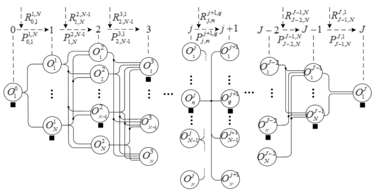
The MDP is applied to capture the EV path selection. The quintuple parameters {T, S, A, P, R} are considered in this study as displayed in Figure 1 [28]. T denotes selection time in a travel chain and J sites, and tj ∈ T is the time when the EV passes through j sites. S presents the scenario and L, sj ∈ S specifies the EV position tj. A presents the actions required at selection time. π represents the route in a travel chain signified by β = {β(sj), j = 0, 1, 2, …, J − 1, sj ∈ S} and EV route β signified by {, , , , …, , ,…, , , }, as depicted in Figure 1. N signifies the position once the EVs arrive at the jth site. To explicitly capture the EV mobility transition from one traffic node to another node, the transition ratio analysis is mandatory. Therefore, P presents the transition ratio to determine EV mobility during route choice at time tj transition from state sj to sj+1:
Assume that the state transition ratio considering EV stochastic route planning is sj = . In addition, suppose that and represent the distance and speed between and sites. The transition ratio is in case EV accomplishes the next site with the least duration, which is higher compared to other transition ratios in a similar state st ∈ {1, 2, …, N}. The ratio of transition is simplified based on the EV’s trip duration between and . Therefore, this phenomenon demonstrates that a more extended trip duration leads to a lower transition ratio, and the ratio of transition is simplified based on the travel period, as follows:
The higher reward means the shortest driving time. Assume R represents the driving time to examine the EV actions based on route selection. In case the itinerary is altered, to with transition ratio , the process can be checked with the reward, as portrayed in Figure 1.
2.3. Electricity Consumption Model
The load mobility is influenced by the traffic scenario and route saturations of the urban transportation system. A traffic-flow model is introduced for capturing the EV speed [29]:
where α1, α2 and α3 are constants; (x) is the traffic movement; Tci,j signifies saturation; and τt designates the road saturation.
Furthermore, the power utilization at different temperature levels is calculated by utilizing the air conditioner (AC) Kpect, and the relative coefficient Ktemp for evaluating power consumption under various temperature scenarios is considered as:
where a1~a4 and b1~b3 are constant values; Temp indicates the temperature; and Kpect signifies different temperatures. Additionally, the decision to alter the AC is examined. A random number k is adopted to uniform distribution considering the various temperature states.
Therefore, considering the influence of AC, power utilization is simplified as:
Furthermore, the state of charge percentage is simplified:
2.4. Charging Demand Modelling Based on Drivers’ Intent
Considering load demand, the charging behavior assumes the travelers prefer to charge randomly, as the state of charge cannot ensure the remaining mileage. Furthermore, the remaining charge is enough. However, as the driver is concerned about the next journey, the driver can charge at the destination. If anxiety ascends, the drivers have a choice of out-of-intent charging.
A fuzzy theory is applied and the power satisfaction Fsat is utilized to formulate the intent of drivers:
Lnext indicates the mileage of the EV’s next trip.
Assume Rfuz represents the charging load and Rfuz(Fsat) is adopted to evaluate the charging behavior, which can be formulated as [19]:
where Rfuz(Fsat) specifies the EV driver charging ratio and analyzes the range concern regarding the journey. Fsat < indicates that there must be charging demand due to the remaining power in case the EVs cannot satisfy the remaining journey. Moreover, a charging ratio deteriorates to zero since the EV has sufficient charge to accomplish the route with Fsat ≥ .
The EV drivers must decide on the charging mode, either slow or fast charging, considering the charging choice:
Further, charging time Tchar is determined and and Tchar are expressed as:
where Lthr specifies the traveling distance SOC,ini to SOC,thr; ∑Lr is the travel time to a threshold and the nth charging station; and nc is the total amount of units transited by drivers once the state of charge declines, SOC,thr.
2.5. Probabilistic Effect on Load Demand
The probabilistic effect can alter the traveling route outcomes. Therefore, the evaluation of the load demand covering various zones comprising a residential zone (RZ), commercial zone (CZ), and working zone (WZ) is simplified as:
where signifies traffic nodes of zone d; the charging load of TNN is signified by (t), zd; is the traffic nodes covering the corresponding zones; and indicates the zone load demand.
2.6. Distribution Network Charging Load Modeling
The interdependence across TNN and DNN based on data information is accumulated, and the load demand is simplified as:
And the power system load is calculated as:
The PDN(t) supply in Z for stopping criterion, and the simulation is ended in case y1 achieves the extreme value W1; otherwise, repeat the charging load demand.
where Zb represents the column vector in matrix Z; is the average value; and δ1 denotes computation precision.
3. Distribution Network Performance Analysis
Considering various realistic factors, load forecasting has a high forecasting accuracy, which was briefly discussed earlier. This section mainly analyzes and forecasts the influence of charging load from distribution networks performance perspectives considering EV high penetrations, hot weather, and high congestion constraints.
3.1. Distribution Network Performance Assessment Indexes
The performance indexes considering per unit value (PUV), fast voltage stability index (FVSI), losses of load probability (LOLP), system average interruption frequency index (SAIFI), system average interruption duration index (SAIDI), and expected energy not supplied (EENS) are adopted for power grid performance evaluation [30]:
where and Vi represent the nominal and actual voltage; Zij and Xij signify the resistance of power transmission; Nb denotes the total amount of simulations; NR is the performance evaluation duration; indicates the disruption at distribution network nodes z; and indicates system losses.
3.2. Distribution Network Performance Analysis through Monte Carlo Simulation
A Monte Carlo simulation is applied to determine components in a distribution network. The failure and repair rates of components are specified as η, σ. An interval of components under different scenarios corresponding to exponential distribution is simplified as [31]:
where φ1 and φ2 are a sequence of random numbers between 0 and 1.
The setup process can be obtained through the state sequence and the duration of the components. The reliability index is estimated based on (19)–(24). The exact computation steps are as follows: first, initialize the information and sample the state series as well as the duration to determine the process conditions. Determine whether the setup is faulty or meets the requirements.
Check if the number of simulation times y2 ranges the maximum value W2. If yes, the process is accomplished:
where ξ, F represents the variance coefficient; U describes an expectation value; νZi represents the Zi performance index during simulations; and δ2 specifies the convergence accuracy.
4. Case Study
4.1. Parameter Settings
This section further explores the features of the proposed study through case studies. An urban transportation network is adopted as an example, and the charging load of an EV in various zones is simulated. The various zones in the transportation network correspond to different nodes, such as RZ (1–16), CZ (24–30), and WZ (17–23), respectively. The transportation network contains 30 nodes and 52 routes corresponding to the main routes. Regarding the distribution network, the IEEE 33 busbar system is applied. The 12,000 population of EVs are considered in the case study. The electrified transportation network nodes’ configuration, capacity, and length of the routes and related parameters are provided in Tables S1–S3 as Supplementary Materials.
4.2. Results and Discussion
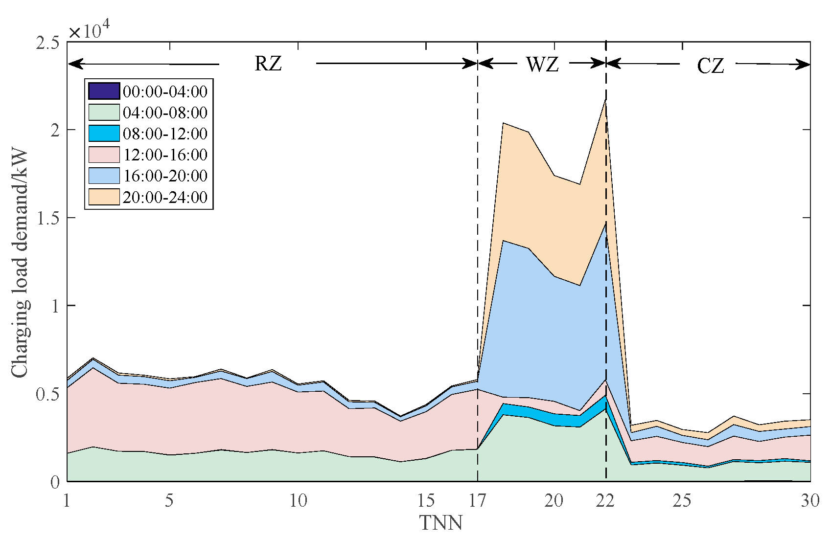
The charging demand simulations for working days and holidays are exhibited in Figure 2. It can be noted that for a working day, the demand of WZ is mostly concentrated between 08:30 and 12:30, and RZ and CZ between 18:00 and 23:00. Moreover, the loads of the three zones remain constant at different time intervals. On the other hand, the charging demand in WZ is nearly zero during holidays, while the other two regions have higher charging demand between 08:00 and 24:00. The peak time on working days and holidays in all zones occurs approximately 2 to 3 h behind the prescribed travel time. Furthermore, jet lag is caused by transportation networks in various locations. Moreover, the typical working day charging load peak demand is almost two times higher than the holidays. This is because 35% of the total EV fleets are not utilized for transportation on holidays, which diminishes the peak demand.
Figure 2.
EV charging demand: (a) working days; (b) holidays.

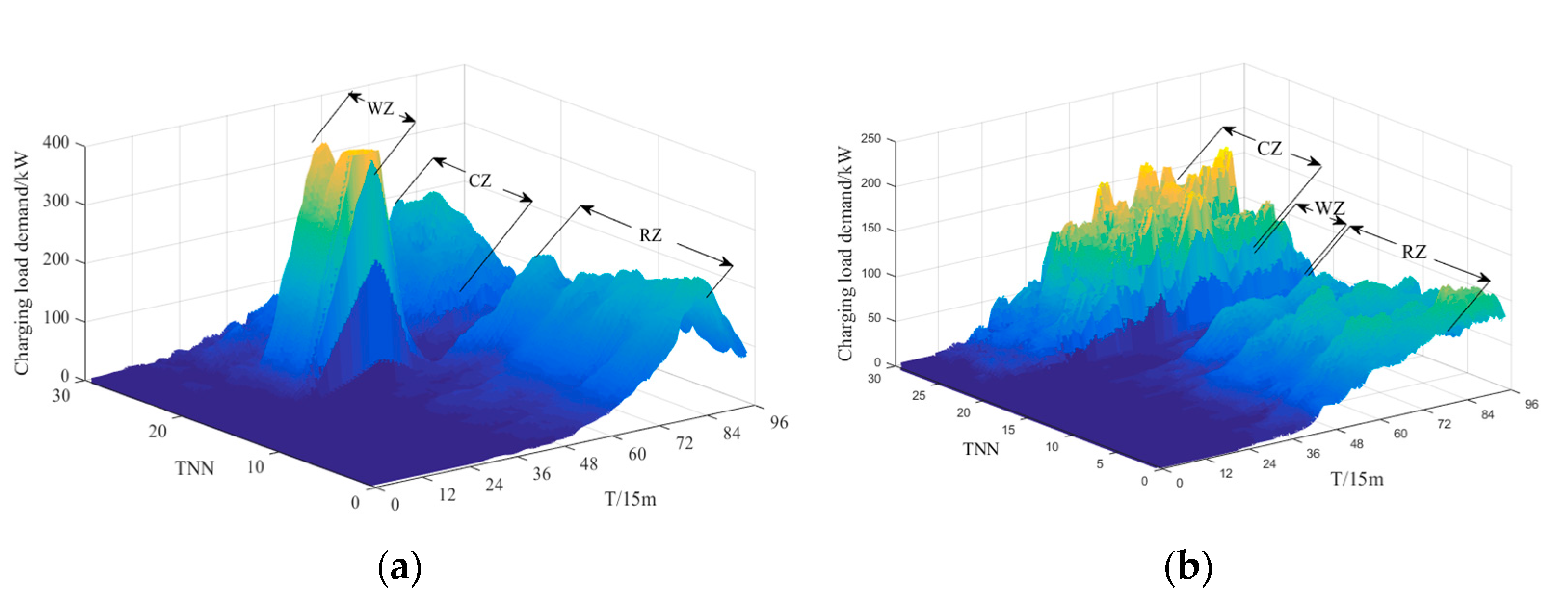
The load demand on hot and congested days is calculated as portrayed in Figure 3. Apart from traveling behavior and hot weather factors, the constraints for both days are similar to the working days. The charging demand on a hot day is similar to a working day. However, the magnitude rises sharply, by about 81.23%, on a hot day. This event happened due to transportation electricity consumption, and additional electricity consumption for AC can increase the charging demand during a hot day. The charging load on a highly congested day is 54.5%, which is higher than a working day. Also, a delay event occurred at RZ and CZ due to the high congestion, causing EV clusters to consume extra traveling time.
Furthermore, the comparative estimation of working day load demand through a stochastic method and the shortest route scheduling through the Dijkstra method is analyzed as shown in Figure 4a. It can be observed that the charging demand of CZ and WZ is significantly less compared to the MDP analysis shown previously. Additionally, the demand concentrated on RZ later at 18:00. Therefore, the proportion was greatly lowered, and the load demand through Dijkstra was 28.43% lower compared to MDP due to the power dissipation brought through the Dijkstra being less than MDP, which can be fulfilled by the initial state of charge. Thus, the charging load during the daytime is reduced. Some drivers charge at RZ once they are back home after a journey. Therefore, charging load regardless of the drivers’ intent is shown in Figure 4b. A spatial–temporal pattern is comparable to the driver’s charging intent case and the load demand also concentrated at RZ during 18:00–24:00. However, load demand with drivers’ intent dropped significantly, and showed a higher demand of approximately 14.23%, indicating that the driver’s behavior significantly affects the load forecasting.
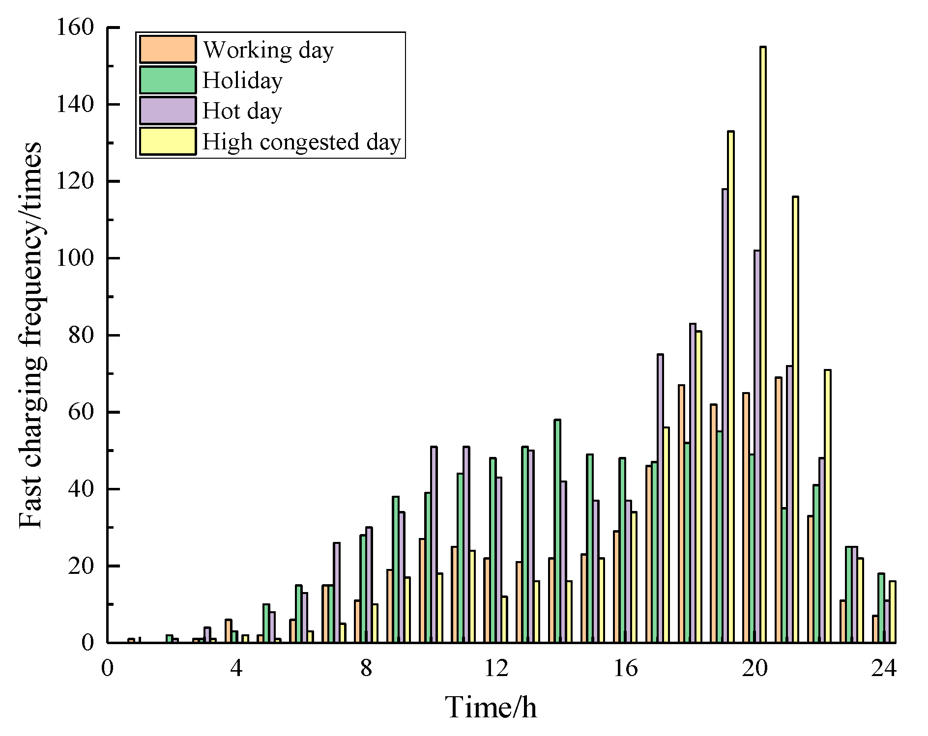
The CZ has a more substantial proportion of fast charging compared to RZ and WZ due to charging time in CZ being scarce and unable to satisfy the load demand. Furthermore, analyzing CZ fast-charging time under four different scenarios can also optimize the operational benefits of the charging system displayed in Figure 5. Fast-charging time on a working day is concentrated between 18:00 and 21:00 during working hours. Moreover, the charging is relatively scattered during holidays between 12:00 and 20:00. The simulation results during highly congested and hot days are similar to the working days. However, the load demand of both days increased intensely due to peak charging demand.
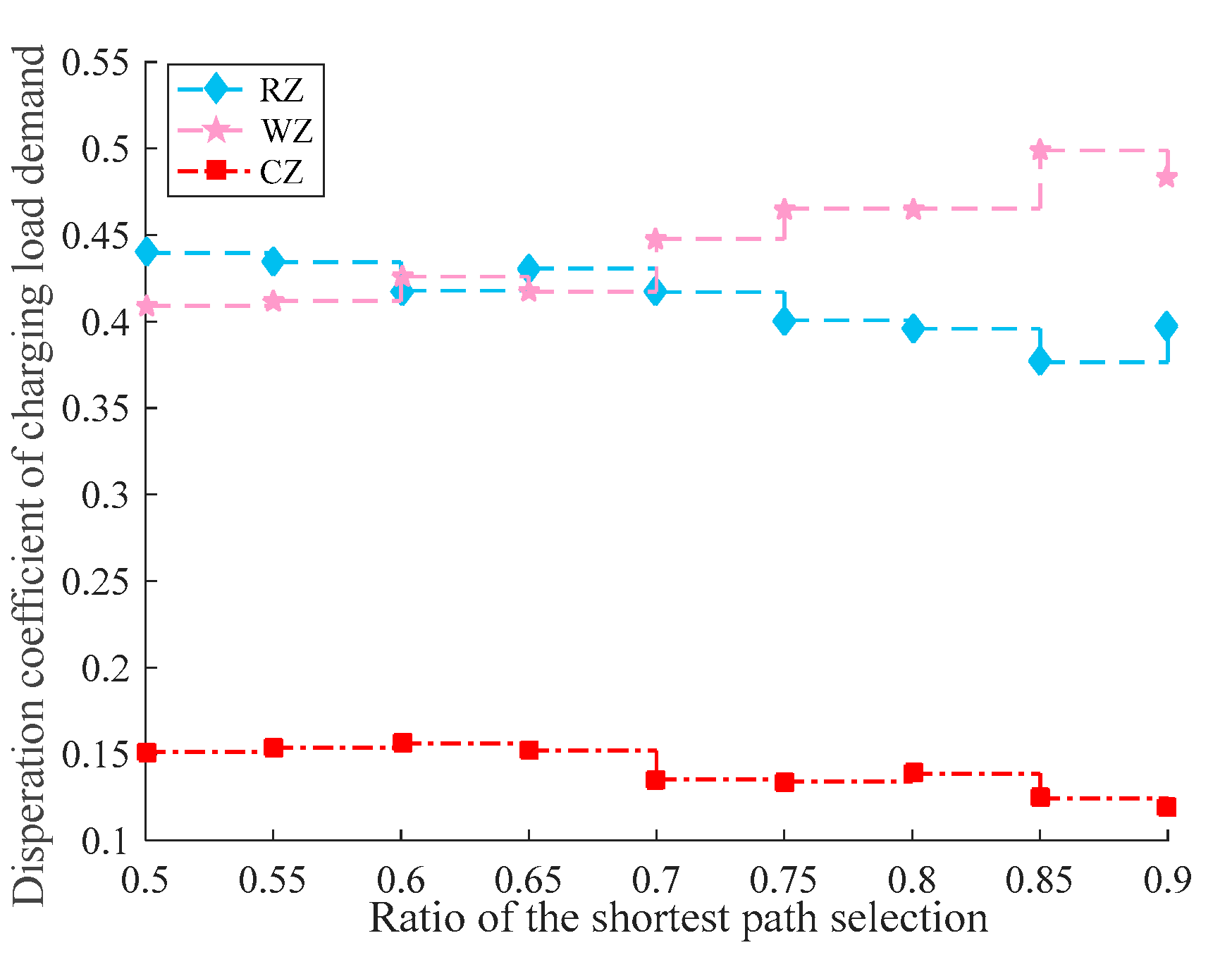
A coefficient disparity is introduced to explicitly analyze the probabilistic effect on the load demand described in Figure 6. As the probabilistic effect increased, there was an overall reduction in RZ and CZ. A contrary event occurred in WZ; the disparity describes that the RZ and CZ demand steadily shifted towards WZ. However, the disparity of corresponding zones was still below zero. Therefore, the dimension of the disparity stipulates that the probabilistic influence on the load partially replicates the forecasting approach.
Furthermore, charging sizing requirements for working days are scrutinized, as depicted in Figure 7. It can be noted that the data are consumption-based, and each unit facilitates a single EV throughout the charging duration, which means the data captures the total numbers being charged simultaneously. Analysis indicates that required charging points are sporadically dispersed, and the quantity of charging units in WZ is twice as many compared to CZ and RZ between 09:00 and 17:00, which also explicates the phenomenon of higher load demand in WZ compared to RZ and CZ during weekdays, as analyzed earlier in Figure 3a. The charging unit demand of RZ and CZ is similar during 17:00–24:00. However, the overall demand in RZ is relatively more significant than in CZ.
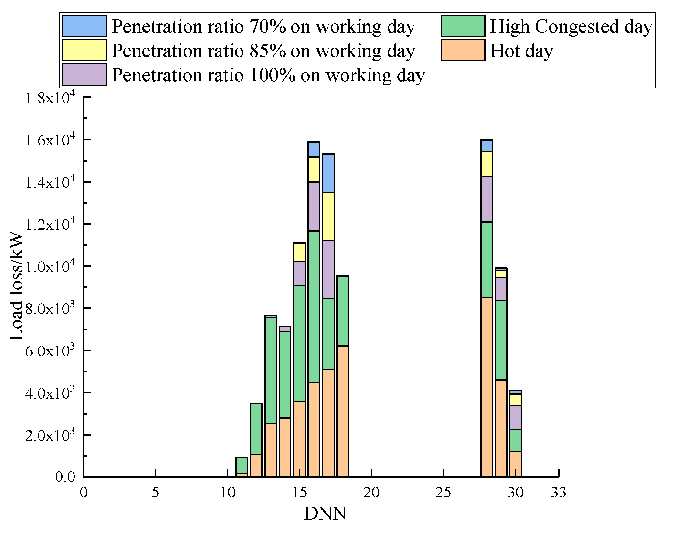
The hot day and highly congested day caused higher charging load demand, as analyzed in Figure 3. The EV high penetrations, high congestion, and weather impact on distribution network performance indicators are quantified as shown in Figure 8 and Table 1, respectively. The high penetrations caused more significant numbers, and indexes of hot days and highly congested days are more extensive than working days. This suggests that the peak load demand led to more fragile distribution stability. The load losses of distribution network nodes are portrayed in Figure 8. The results reveal that higher penetration, hot weather, and high congestion caused greater losses and a rapidly increased load demand. Likewise, the losses diminished in nodes 15–18 and 27–30. However, if the system infrastructure is well established with relevant emergency demand responses, the system’s performance can be optimized, lending additional support to the power system.
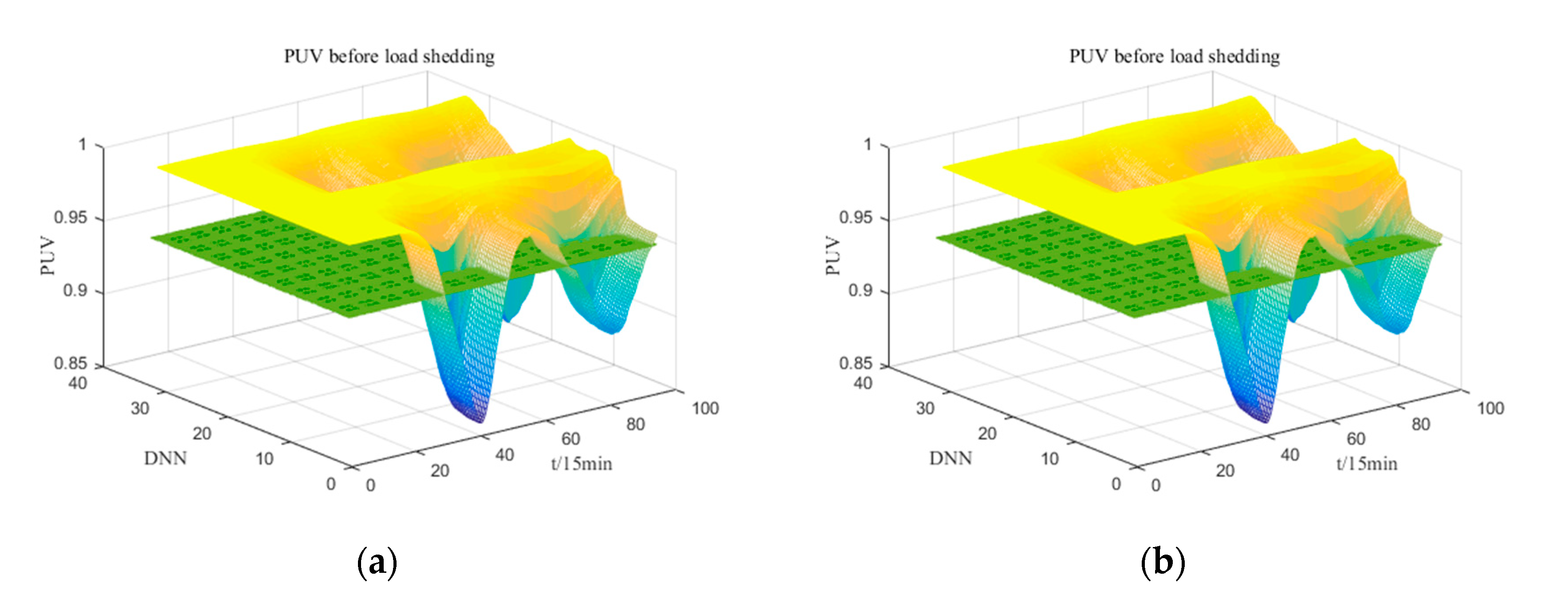
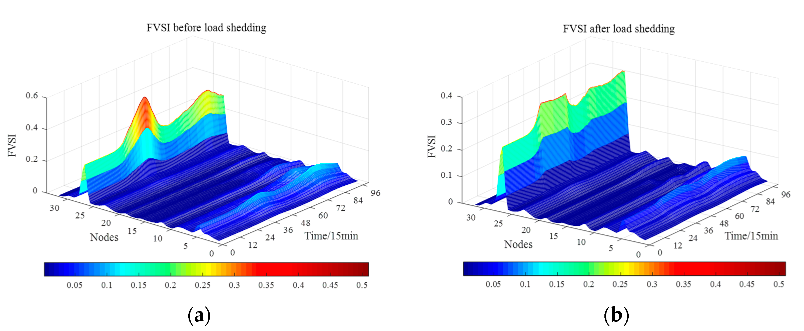
Finally, load demand influence for power system performance perspectives is explicitly quantified through PUV and FVSI. Figure 9 and Figure 10 show the values of distribution network nodes, demonstrating that higher FVSI values caused higher losses in the distribution network. From Figure 9a,b, it can be observed that the five charging scenarios have similar voltage drop events during 7:00–12:00 and 17:00–23:00. Therefore, during this period, the distribution network relies on nodes 7–18 and 27–33 because of severe voltage drops. The continued deterioration of PUVs happens due to massive EV penetration and increased high temperature and congestion constraints. Likewise, the overall upward event occurred to the FVSI, as shown in Figure 10a,b. The higher FVSI leads to intensifying EV penetration as well as emergencies of hot days and high congestion, thus deteriorating overall system performance. Consequently, lower FVSI leads to optimal performance of the system.
5. Conclusions and Future Work
The ambiguity of electrical vehicles charging load affects the coupled power and transportation networks’ performance. A spatial–temporal forecasting strategy of EV charging demand and performance assessment of the power systems perspectives is analyzed in this paper. The EVs’ load mobility as well as stochastic path selection are captured through the proposed model. Additionally, the performance assessment method of the distribution system effectively determines the load effect under various states considering the numerous indexes. The case studies revealed that the proposed model can robustly capture the charging schedule. Furthermore, load forecasting analysis demonstrates the real-world scenario by explicitly evaluating factors including load mobility, path selection, traffic flow, drivers’ behavior, and hot weather. Also, the travel chain mechanisms and driving behavior caused significant differences in load distributions in various scenarios. The hot weather and high congestion caused significant load demands, and the charging delay happened during a highly congested day. The significant EV integration, traffic congestion, and hot weather lead to higher load losses, which may compromise the performance and safe operation of the coupled power-transportation networks. In our future work, the proposed study can be further expanded to explicitly analyze optimal charging sitting and sizing to reduce the charging delay during peak demand. Furthermore, determines the coupled power and transportation networks’ price mechanisms and dynamic power and traffic flow constraints under various scenarios.
Supplementary Materials
The following supporting information can be downloaded at: https://0-www-mdpi-com.brum.beds.ac.uk/article/10.3390/en16135178/s1, Table S1: Parameters of urban electrified transportation networks; Table S2: Capacity of the road during different periods; Table S3: Length of the roads.
Author Contributions
Conceptualization, S.J. and J.L.; writing—original draft, S.J.; writing—review and editing, S.J. and J.L. All authors have read and agreed to the published version of the manuscript.
Funding
This work was supported by the Basic Theory and Key Technologies of Competitive Electricity Sales Service Market [Grant No. U2066209].
Data Availability Statement
The data presented in this study are available upon request.
Conflicts of Interest
The authors declare no conflict of interest.
References
- Outlook, IEA Global EV. 2022. Available online: https://www.iea.org/commentaries/electric-cars-fend-off-supply-challenges-to-more-than-double-global-sales (accessed on 10 December 2022).
- Rautiainen, A.; Repo, S.; Jarventausta, P.; Mutanen, A.; Vuorilehto, K.; Jalkanen, K. Statistical charging load modeling of PHEVs in electricity distribution networks using national travel survey data. IEEE Trans. Smart Grid 2012, 3, 1650–1659. [Google Scholar] [CrossRef]
- Tehrani, N.H.; Wang, P. Probabilistic estimation of plug-in electric vehicles charging load profile. Electr. Power Syst. Res. 2015, 124, 133–143. [Google Scholar] [CrossRef]
- Ul-Haq, A.; Azhar, M.; Mahmoud, Y.; Perwaiz, A.; Al-Ammar, E.A. Probabilistic modeling of electric vehicle charging pattern associated with residential load for voltage unbalance assessment. Energies 2017, 10, 1351. [Google Scholar] [CrossRef] [Green Version]
- Ul-Haq, A.; Cecati, C.; El-Saadany, E. Probabilistic modeling of electric vehicle charging pattern in a residential distribution network. Electr. Power Syst. Res. 2018, 157, 126–133. [Google Scholar] [CrossRef]
- Jawad, S.; Liu, J. Electrical vehicle charging services planning and operation with interdependent power networks and transportation networks: A review of the current scenario and future trends. Energies 2020, 13, 3371. [Google Scholar] [CrossRef]
- Luo, Y.; Zhu, T.; Wan, S.; Zhang, S.; Li, K. Optimal charging scheduling for large-scale EV (electric vehicle) deployment based on the interaction of the smart-grid and intelligent-transport systems. Energy 2016, 97, 359–368. [Google Scholar] [CrossRef]
- Shao, C.; Wang, X.; Wang, X.; Du, C.; Wang, B. Hierarchical Charge Control of Large Populations of EVs. IEEE Trans. Smart Grid 2015, 7, 1147–1155. [Google Scholar] [CrossRef]
- Su, S.; Zhao, H.; Zhang, H.; Lin, X.; Yang, F.; Li, Z. Forecast of electric vehicle charging demand based on traffic flow model and optimal path planning. In Proceedings of the 2017 19th International Conference on Intelligent System Application to Power Systems (ISAP), San Antonio, TX, USA, 17–20 September 2017; pp. 1–6. [Google Scholar] [CrossRef]
- Minelli, S.; Izadpanah, P.; Razavi, S. Evaluation of connected vehicle impact on mobility and mode choice. Traffic Transp. Eng. 2015, 2, 301–312. [Google Scholar] [CrossRef] [Green Version]
- Qian, K.; Zhou, C.; Allan, M.; Yuan, Y. Modeling of load demand due to ev battery charging in distribution systems. IEEE Trans. Power Syst. 2010, 26, 802–810. [Google Scholar] [CrossRef]
- Wang, T.-G.; Xie, C.; Xie, J.; Waller, T. Path-constrained traffic assignment: A trip chain analysis under range anxiety. Transp. Res. Part C Emerg. Technol. 2016, 68, 447–461. [Google Scholar] [CrossRef]
- Tang, D.; Wang, P. Nodal impact assessment and alleviation of moving electric vehicle loads: From traffic flow to power flow. IEEE Trans. Power Syst. 2016, 31, 4231–4242. [Google Scholar] [CrossRef]
- Wang, Y.; Infield, D. Markov Chain Monte Carlo simulation of electric vehicle use for network integration studies. Int. J. Electr. Power Energy Syst. 2018, 99, 85–94. [Google Scholar] [CrossRef]
- Zhang, H.; Hu, Z.; Xu, Z.; Song, Y. An integrated planning framework for different types of pev charging facilities in urban area. IEEE Trans. Smart Grid 2015, 7, 2273–2284. [Google Scholar] [CrossRef]
- Wang, X.; Shahidehpour, M.; Jiang, C.; Li, Z. Coordinated planning strategy for electric vehicle charging stations and coupled traffic-electric networks. IEEE Trans. Power Syst. 2018, 34, 268–279. [Google Scholar] [CrossRef]
- Hong, L.; Xu, Z.; Chang, L. Timing interactive analysis of electric private vehicle traveling and charging demand considering the sufficiency of charging facilities. Proc. CSEE 2018, 38, 5469–5478. [Google Scholar]
- Liu, K.; Liu, Y. Stochastic user equilibrium based spatial-temporal distribution prediction of electric vehicle charging load. Appl. Energy 2023, 339, 120943. [Google Scholar] [CrossRef]
- Lv, S.; Wei, Z.; Sun, G.; Chen, S.; Zang, H. Optimal power and semi-dynamic traffic flow in urban electrified transportation networks. IEEE Trans. Smart Grid 2019, 11, 1854–1865. [Google Scholar] [CrossRef]
- Wang, H.; Fang, Y.-P.; Zio, E. Risk assessment of an electrical power system considering the influence of traffic congestion on a hypothetical scenario of electrified transportation system in New York state. IEEE Trans. Intell. Transp. Syst. 2019, 22, 142–155. [Google Scholar] [CrossRef]
- Rezaee, S.; Farjah, E.; Khorramdel, B. Probabilistic analysis of plug-in electric vehicles impact on electrical grid through homes and parking lots. IEEE Trans. Sustain. Energy 2013, 4, 1024–1033. [Google Scholar] [CrossRef]
- Clairand, J.M.; Rodríguez-García, J.; Alvarez-Bel, C. Smart charging for electric vehicle aggregators considering users’ preferences. IEEE Access 2018, 6, 54624–54635. [Google Scholar] [CrossRef]
- Ahmad, F.; Iqbal, A.; Ashraf, I.; Marzband, M.; Khan, I. Optimal location of electric vehicle charging station and its impact on distribution network: A review. Energy Rep. 2022, 8, 2314–2333. [Google Scholar] [CrossRef]
- Kizhakkan, A.R.; Rathore, A.K.; Awasthi, A. Review of electric vehicle charging station location planning. In Proceedings of the 2019 IEEE Transportation Electrification Conference (ITEC-India), Bengaluru, India, 17–19 December 2019; pp. 1–5. [Google Scholar]
- Kaya, Ö.; Alemdar, K.D.; Campisi, T.; Tortum, A.; Çodur, M.K. The Development of decarbonisation strategies: A three-step methodology for the suitable analysis of current Evcs locations applied to Istanbul, Turkey. Energies 2021, 14, 2756. [Google Scholar] [CrossRef]
- Zhang, Q.; Zhu, Y.; Wang, Z.; Su, Y.; Li, C. Reliability assessment of distribution network and electric vehicle considering quasi-dynamic traffic flow and vehicle-to-grid. IEEE Access 2019, 7, 131201–131213. [Google Scholar] [CrossRef]
- Liu, G.; Kang, L.; Luan, Z.; Qiu, J.; Zheng, F. Charging station and power network planning for integrated electric vehicles (EVs). Energies 2019, 12, 2595. [Google Scholar] [CrossRef] [Green Version]
- Caro-Ruiz, C.; Al-Sumaiti, A.S.; Rivera, S.; Mojica-Nava, E. A mdp-based vulnerability analysis of power networks considering network topology and transmission capacity. IEEE Access 2019, 8, 2032–2041. [Google Scholar] [CrossRef]
- Liu, C.; Wang, J.; Cai, W.; Zhang, Y. An energy-efficient dynamic route optimization algorithm for connected and automated vehicles using velocity-space-time networks. IEEE Access 2019, 7, 108866–108877. [Google Scholar] [CrossRef]
- Wei, W.; Zhou, Y.; Zhu, J.; Hou, K.; Zhao, H.; Li, Z.; Xu, T. Reliability assessment for ac/dc hybrid distribution network with high penetration of renewable energy. IEEE Access 2019, 7, 153141–153150. [Google Scholar] [CrossRef]
- Su, S.; Hu, Y.; He, L.; Yamashita, K.; Wang, S. An assessment procedure of distribution network reliability considering photovoltaic power integration. IEEE Access 2019, 7, 60171–60185. [Google Scholar] [CrossRef]
Figure 1.
Transportation network schematic overview.

Figure 3.
EV charging demand: (a) hot day; (b) highly congested day.

Figure 4.
EV working day charging demand: (a) considering drivers’ intent; (b) regardless of drivers’ intent.
Figure 4.
EV working day charging demand: (a) considering drivers’ intent; (b) regardless of drivers’ intent.

Figure 5.
Commercial zone charging frequency under different states.

Figure 6.
Driving route selection and charging power disparity coefficient correlation.

Figure 7.
Charging sizing evaluation in different zones.

Figure 8.
Distribution network load losses under different charging states.

Figure 9.
PUV analysis under different charging scenarios: (a) before load shedding; (b) after load shedding.
Figure 9.
PUV analysis under different charging scenarios: (a) before load shedding; (b) after load shedding.

Figure 10.
FVSI analysis under different charging states: (a) before load shedding; (b) after load shedding.
Figure 10.
FVSI analysis under different charging states: (a) before load shedding; (b) after load shedding.


Table 1.
Performance indicators of the power system under different charging states.
| Scenarios | LOLP (Year) | SAIFI (t/Year) | SAIDI (h/Year) | IEENS (MWh/Year) |
|---|---|---|---|---|
| With 70% penetration during working day | 0.004252 | 13.5853 | 4.5835 | 37.1596 |
| With 85% penetration during working day | 0.004371 | 13.9235 | 4.8358 | 40.4833 |
| With 100% penetration during working day | 0.004401 | 14.6854 | 5.2136 | 45.1584 |
| Highly congested day | 0.004477 | 14.9158 | 5.3234 | 51.7656 |
| Hot day | 0.004512 | 14.9647 | 5.3743 | 54.8174 |
Disclaimer/Publisher’s Note: The statements, opinions and data contained in all publications are solely those of the individual author(s) and contributor(s) and not of MDPI and/or the editor(s). MDPI and/or the editor(s) disclaim responsibility for any injury to people or property resulting from any ideas, methods, instructions or products referred to in the content. |
© 2023 by the authors. Licensee MDPI, Basel, Switzerland. This article is an open access article distributed under the terms and conditions of the Creative Commons Attribution (CC BY) license (https://creativecommons.org/licenses/by/4.0/).
Share and Cite
MDPI and ACS Style
Jawad, S.; Liu, J. Electrical Vehicle Charging Load Mobility Analysis Based on a Spatial–Temporal Method in Urban Electrified-Transportation Networks. Energies 2023, 16, 5178. https://0-doi-org.brum.beds.ac.uk/10.3390/en16135178
AMA Style
Jawad S, Liu J. Electrical Vehicle Charging Load Mobility Analysis Based on a Spatial–Temporal Method in Urban Electrified-Transportation Networks. Energies. 2023; 16(13):5178. https://0-doi-org.brum.beds.ac.uk/10.3390/en16135178
Chicago/Turabian StyleJawad, Shafqat, and Junyong Liu. 2023. "Electrical Vehicle Charging Load Mobility Analysis Based on a Spatial–Temporal Method in Urban Electrified-Transportation Networks" Energies 16, no. 13: 5178. https://0-doi-org.brum.beds.ac.uk/10.3390/en16135178
Note that from the first issue of 2016, this journal uses article numbers instead of page numbers. See further details here.