
Dynamic Pricing Based on Demand Response Using Actor–Critic Agent Reinforcement Learning

Faculty of Electrical and Electronics Engineering, Yildiz Technical University, Davutpasa Campus, Esenler, 34220 Istanbul, Turkey
*
Authors to whom correspondence should be addressed.
Energies 2023, 16(14), 5469; https://0-doi-org.brum.beds.ac.uk/10.3390/en16145469
Submission received: 18 June 2023
/
Revised: 5 July 2023
/
Accepted: 17 July 2023
/
Published: 19 July 2023
(This article belongs to the Topic Energy Consumption, Demand and Price Forecasting with Artificial Intelligence)
Abstract
:Eco-friendly technologies for sustainable energy development require the efficient utilization of energy resources. Real-time pricing (RTP), also known as dynamic pricing, offers advantages over other pricing systems by enabling demand response (DR) actions. However, existing methods for determining and controlling DR have limitations in managing an increasing demand and predicting future pricing. This paper presents a novel approach to address the limitations of existing methods for determining and controlling demand response (DR) in the context of dynamic pricing systems for sustainable energy development. By leveraging actor–critic agent reinforcement learning (RL) techniques, a dynamic pricing DR model is proposed for efficient energy management. The model’s learning framework was trained using DR and real-time pricing data extracted from the Australian Energy Market Operator (AEMO) spanning a period of 17 years. The efficacy of the RL-based dynamic pricing approach was evaluated through two predicting cases: actual-predicted demand and actual-predicted price. Initially, long short-term memory (LSTM) models were employed to predict price and demand, and the results were subsequently enhanced using the deep RL model. Remarkably, the proposed approach achieved an impressive accuracy of 99% for every 30 min future price prediction. The results demonstrated the efficiency of the proposed RL-based model in accurately predicting both demand and price for effective energy management.
1. Introduction
1.1. Motivation and Background
With the development of the recent sophisticated technologies in sustainable energy systems, demand response (DR) emerged as an efficient process to reduce energy costs and real-time pricing because of the quick reaction ability to supply–demand imbalance [1,2]. DR refers to a tariff or procedure implemented to incentivize adjustments in energy pricing or offer incentive costs with the aim of promoting lower energy consumption during periods of high market prices or when grid reliability is at risk [3].
In the existing scientific literature, DR is commonly classified into two categories: price-based DR and incentive-based DR [4]. Price-based DR urges consumers to shift their energy consumption practices in response to variable energy costs, whereas incentive-based DR offers users with flat or dynamic incentives to reduce energy consumption during periods of system overload [5]. Each category has its own unique advantages and potential considerations for achieving effective demand management. However, this research primarily focuses on price-based DR, which has been extensively investigated in previous studies, as depicted in Figure 1 along with other subcategories [6,7,8]. Price-based DR imparts excellent features, such as accessibility, reliability, and rapidity. The example study explored the influence of demand response on the improvement of reliability [9]. A notable pricing program is a peak price-based DR method that operates at a certain crucial period when electricity systems sense emergencies [10].
Dynamic pricing (real-time pricing) has gained much attention among price-based DR programs, since it creates a relationship between a supplier and customers by explaining a logical reaction to the competition [11]. It is also a successful solution for utilities to grow their competitiveness and retain their consumers [12,13]. Prediction is a vital component of the energy management system. Modeling the dynamic prices needs predictions of the prospect demands, whereas scheduling needs future price predictions. Predictions thus provide a prospect planning policy for dynamic tariffs and also help consumers to plan energy utilization during dynamic pricing situations. This price-based demand response program allows customers to save money by reducing peak electricity demand. Customers who sign up for this program may receive a cash incentive or credit every month and can use it to lower their monthly bills by reducing their peak electricity usage. The study in [14] developed price prediction models based on dynamic regression and transfer function solutions by using data from Spain and California, achieving a high accuracy; however, limitations of ARIMA models on the data from the same sources are observed in [15]. ARIMA models are used to predict Ontario’s hourly prices from the accessible source with a significant accuracy [16] but failed in predicting unusually high or low prices. Artificial Neural Networks (ANNs) based on the method used by Mandal et al. [16] showed a better prediction accuracy. In [16], various factors including demand, history, and time are identified, which influence price prediction. Neural-network-based next-day price prediction displayed a satisfactory accuracy to support request policy decisions [17]. A kernel-based next-day prediction model was studied and has proven its effectiveness.
Accurate demand forecasting is essential for energy-supply systems to successfully plan their supply and generation capacity. These forecasts can include a range of time periods, including daily, weekly, monthly, and yearly projections. Short-term forecasts, spanning from minutes to several hours in advance, are especially useful for real-time control and scheduling of power systems. Long-term forecasting, on the other hand, is critical for simplifying investment planning and maintenance scheduling. Various solutions to predict the long-term energy demands are evaluated in terms of accuracy where simple and robust solutions outperformed. Double seasonal Holt Winters exponential smoothening is implemented for the day and week seasonality. This solution showed an effective solution as compared to ARIMA and the standard Holt Winters method for short-term demand prediction [18]. A recent study in [18] introduces an extension to [19] incorporating the year seasonal cycle into their model. This extended model demonstrated a superior performance compared to both the double seasonal model and the univariate neural network solution. Furthermore, [20] presents evidence that utilizing single-order moving average smoothened data in an E-Support Vector Regress (E-SVR) model can effectively reduce prediction errors. Another study [21] focuses on incorporating weather factors into medium-term energy demand prediction. By integrating various weather factors with an autoregressive model, they successfully mitigate serial correlation across four distinct climatic scenarios. Various weather factors are used along with an autoregressive model to reduce serial correlation for four different climatic scenarios. In [22], the Trigonometric Gray Model (TGM) prediction model improved the prediction accuracy. Gray prediction along with the rolling mechanism in [23] predicted Turkish energy demand with limited data and less computational effort. Semi-parametric additive models are used to estimate the relationship between energy demand and other independent variables [24]. The probabilistic model is proposed in [25] to predict energy demand from simulated weather data. Multiple linear regression and ANNs are applied in [26] with principal components to predict energy demand. The price and demand prediction using neural models is depicted in Figure 2.
While the current literature effectively presents an overview of demand response (DR) systems, there remains an essential gap in how these systems are practically implemented, specifically in terms of dynamic pricing. Numerous studies have focused on the conceptual basis of price-based DR, illuminating its potential benefits such as an improved accessibility, reliability, and rapid response [6,7,8]. However, the practical integration of dynamic pricing, a crucial subset of price-based DR, is largely understudied.
Moreover, most existing research is based on theoretical models, which may not accurately represent the complexities and nuances of real-world energy management systems. These models often overlook unpredictable variables such as sudden changes in energy demand or supply, resulting in a disconnection between theory and practice.
This paper seeks to address these limitations by providing a comprehensive exploration of dynamic pricing within real-world DR systems. Our research will build upon existing theoretical foundations, adding a layer of practical understanding. The goal is to bridge the gap between theoretical models and practical applications, enhancing the effectiveness of dynamic pricing in reducing energy costs and improving grid reliability. This research will also shed light on how predictions can be effectively utilized in planning and implementing dynamic pricing strategies, offering a valuable contribution to the existing body of knowledge.
1.2. Contributions and Organization
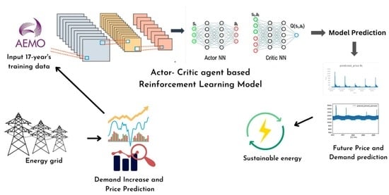
Reinforcement learning has gained prominence as a robust methodology for enhancing the efficiency of energy management system (EMS) operations when confronted with dynamic factors, e.g., varying prices of energy and utilization patterns. This research presents a new approach to dynamic-pricing demand response (DR) for energy management, leveraging reinforcement learning techniques. The proposed model adopts an actor–critic agent framework trained on demand response and real-time pricing (RTP) data. The learning process incorporates a 17-year dataset obtained from the Australian Energy Market Operator (AEMO), enabling the model to accurately forecast future energy demand and pricing patterns.
The evaluation of the RL-based dynamic pricing approach in this study focuses on two prediction scenarios: actual/predicted demand and actual/predicted price. The former assesses the accuracy of demand prediction by comparing actual energy demand with the model-generated predictions. Similarly, the latter evaluates the model’s ability to forecast future energy prices by comparing actual prices with the predicted values. The results demonstrate that the proposed model excels in accurately predicting both demand and price, making it suitable for effective energy management.
Demand and price data ranging from 1999 to 2015 obtained from New South Wales (NSW) was used to train the model, enabling it to predict future energy demand and prices based on the behavior and characteristics of the AEMO. This capability proves valuable for analyzing future energy demand patterns, understanding long-term trends, estimating energy requirements for future power plants, and studying future pricing dynamics. The present study makes a unique contribution by developing a deep reinforcement learning model particularly tailored for dynamic-pricing demand response. Furthermore, it uses a 17-year pricing and demand database as a training resource, incorporating both historical and real-time data to improve demand and price forecasts.
The rest of this paper is structured as follows. The actor–critic agent-based reinforcement learning for the prediction of demand and price is presented in Section 2. Simulations are presented in Section 3. Results and discussions are given in Section 4. Finally, conclusions are presented in Section 5.
1.3. Literature Review
Several studies have been proposed to study price-based DR, and with price-based demand response, electricity usage can be reduced during times of peak demand. For example, in [27,28], the energy utilization forecast of housing appliances was examined using time-of-use pricing to minimize the costs of customers and improve the efficiency of energy. Correspondingly, the study in [29] examined the influence of large-scale field exploitation of obligatory time-of-use pricing of industrial and commercial customers on energy utilization. DR associated with industrial and commercial customers during vital peak pricing is examined in [30] where the duration and time of the price raise were prearranged. The studies [31,32,33,34,35,36] reported deterministic DR models with next-day pricing for customers, where the next-day energy pricing is established a priori and optimized energy utilization scheduling was predefined via reducing per-day costs. Two solutions, real-time-incentive-based and next-day-pricing-based for large energy customers were proposed in [37]; however, the time duration and incentive rate value were inferred before scheduling.
A study conducted in [38] introduced price-based demand response (DR) methods for industrial loads, enabling control over both current and future load scheduling. However, incorporating future price uncertainty into real-world conditions posed challenges in the modeling process.
The above-presented studies conclude that the operation of energy management systems, which depends on typical solutions such as deterministic policies and theoretical models, undergoes two main problems: (i) involving the deterministic policies to operate the non-stationary systems cannot assure optimization, and the alteration in variables can lead to a consequence in cost, and (ii) theoretical models typically approximate the real situation and consequently may be impractical as compared to the real energy management systems. Theoretical models are essential for conceptualizing complex systems. However, they often simplify reality, leading to discrepancies when applied to practical scenarios like energy management systems. Simplification aids in isolating key variables, yet overlooks unpredictable real-world elements like weather extremes or technical malfunctions. Moreover, models often assume idealized conditions, such as a perfect energy transfer efficiency, rarely reflected in practice. Hence, while theoretical models provide important insights, their inherent approximations can limit their direct applicability to real-world energy management systems. The emergence of artificial intelligence (AI) has spurred an increasing interest in the application of reinforcement learning techniques for addressing decision-making challenges in smart grid systems. Developments in reinforcement learning have been recorded as a particularly deep Q-network in AlphaGo and Atari [39,40].
2. Materials and Methods
Reinforcement learning (RL), a machine learning approach, is involved in the process of how a software agent takes actions in a stochastic situation to boost some assumption of a growing reward as shown in Figure 3 [41]. In RL, an agent connects to its environment, and at each time step, it chooses an action from the available options, which is then transmitted to the environment. Following that, an agent is rewarded, and the environment develops to new states.
In [41,42,43,44], RL models were employed for energy scheduling in storage systems and achieved optimized charging/discharging policies. The studies in [45,46,47] used RL for achieving energy management for certain demand response appliances such as thermostat-controlled loads, electric water heaters, and more. A fully automated energy management system for DR rescheduling as a RL problem was proposed in [48] where RL significantly solved the problem over device clusters. A model-free batch RL model combined with a market-based heuristic was proposed in [42] for energy rescheduling. The study in [49] formulated a fundamental sequential decision-making problem as a Markov decision process and employed RL for energy management. The study in [50] considered microgrids, where every microgrid can acquire or distribute energy to other microgrids. The RL was employed among microgrids to select an acquiring/distributing energy trading strategy such that average income will increase. RL in ref. [51] is employed to show the hierarchical decision-making structure where a discrete finite Markov decision procedure and Q-learning are implemented to solve dynamic pricing. The elasticity of energy demand is discussed in various studies [11,52,53,54]. The elasticity of energy demand is a measure of the responsiveness of energy demand to changes in price. It is calculated as the percentage change in units of energy demanded associated with a one percent change in price. Table 1 summarizes different models for energy price and demand prediction.
2.1. Proposed Dynamic-Pricing-Based Demand Response Approach
In this section, the proposed dynamic-pricing-based demand response is explained. With dynamic-pricing-based DR, you can automatically lower your energy consumption when prices are high or increase it during off-peak times of the day. The actor–critic agent RL is employed to perform the dynamic-pricing demand response. The agent is capable of predicting the load change based on history as well as external factors such as weather, customer activity, and price. It uses this prediction to decide how much energy it should buy from the grid at any given time. Firstly, the system model is explained. Secondly, the actor–critic agent RL for the task is explained.
2.1.1. System Model
A hierarchy of the power system operation model is depicted in Figure 4, which is comprised of a grid operator, a service provider, and end customers. The installation, management, and maintenance of the national high-voltage energy grid are operated by grid operators, where low-voltage energy is transmitted by the service provider. The service provider receives energy from the grid operator at wholesale market rates and sells it to end users at retail market prices. This study emphasizes the demand response algorithm for forecasting future prices and energy consumption.
2.1.2. Actor–Critic Agent RL for Demand Response
During actor–critic training, first, the initial state is received; afterward, the actor selects the price for the next step. The critic component evaluates the disparity between the modeled demand predicted for the subsequent step and the actual demand given a new price. The critic is retrained with respect to the difference between its prediction and the model’s prediction. An actor is retrained to enforce or weaken its leaning to replicate the same action in similar conditions depending on the critic’s result. This arrangement allows the critic to examine the states with respect to the previous model’s information, which is reliable but diverges from the real data. The actor adapts to price fluctuations to align the critic’s return with zero, signifying the close match between expected and required demand. At each time step t, the RL framework facilitates ongoing interaction between the agent and the environment, through state s(t), action a(t), and reward r(t). The agent observes the current state s(t) based on the variable set and subsequently selects an action, a(t), accordingly. The environment, in turn, accepts the chosen action a(t) and transitions to a new state, s(t + 1). The reward r(t + 1) related to transition (s(t), a(t), s(t + 1)) is determined. The aim of the RL agent is to learn the policy P, λ: A × S → [0, 1], such that
Policy P increases the expected cumulative reward. The agent maximizes the expected cumulative reward at each step G as
The conventional approach models the sequential decision-making problem as a Markov decision process (MDP) where the environment is described with transition probabilities. In this study, a continuous environment was employed and the model probabilities of the environment were computed using recurrent neural networks (RNNs). An RNN uses model outputs at each training epoch and appends to the new model input, which makes RNNs appropriate for time-series prediction. With the inputs and outputs of an RNN model as the vectors x(t) and y(t), the model contains three connection weight matrices, that is, W(ih), W(hh), and W(ho) with the hidden and output units as well as the activation functions of f(h) and f(o). An RNN’s actions may be characterized as a dynamical system using a pair of nonlinear matrix equations:
where h(t) represents the hidden unit and activations set, which keeps the current states of the model. During training, the model takes input samples sequentially, obtaining the next input sample as output. The difference between the actual output and prediction (E) is passed through the network layers backward and network weights are updated due to the gradient descent rule where δ is the learning rate selected to make model training slighter.
The RNN-based actor–critic algorithm is used to partially observe the Markov decision process with continuous outputs. The actor–critic is an improved policy gradient technique where a policy function selects an action and then model feedback improves the value function. The policy function P or an actor takes the current state s(t) and returns the energy price for the next time step a(t + 1). For example, in a single-agent RL scenario, the actor (user) will look at its state(s) and use this information to decide how much power to consume or return. When the price changes, the environment model creates a the new state s(t + 1) and reward r(t + 1). The value function (Vf) or the critic predicts the expected reward e(t + 1) and trains on the actual demand r(t + 1) for the subsequent state. The actor updates its model of the environment and makes decisions based on this updated knowledge. The critic is a reinforcement learning model, which provides feedback on how close the actor’s estimates are to the true value given by the environment. This discrepancy is used as the temporal-difference error to increase or decrease the actor’s leaning to prefer the same price in a similar state by fitting its learning rate κ where the training sample is the price it recommended in the previous step. The weights of critics are updated on temporal-difference errors directly using a gradient step with respect to these errors. The process is represented in Figure 5.
3. Model and Simulation
3.1. Data Collection
The research data utilized in this study are sourced from the Australian Energy Market Operator (AEMO) [21]. AEMO is responsible for managing electricity and gas systems and markets in Australia, ensuring access to affordable, secure, and reliable energy. AEMO houses a comprehensive dataset encompassing all Australian states, updated every 30 min over the past 20 years, encompassing energy demand and prices. This dataset represents real-time demand and pricing information. For this paper, the case study focuses on the state of New South Wales (NSW). The dataset for NSW comprises 21 years, spanning from 1999 to 2020, containing historical records of energy demand and price variations over multiple years. The demand level is regulated by price, aiming to maintain a stable operation of the power system. To automate this feedback model, a reinforcement learning algorithm is employed, utilizing only objective variables from previous steps as inputs. The dataset is divided into two parts: the first part, encompassing data from 1999 to 2015, is utilized for training the model, while the second part, covering data from 2016 to 2020, serves for testing the model’s efficiency, accuracy, and comparison with actual results obtained from AEMO. No auxiliary data are utilized in the model development process, ensuring a reliance on objective variables and historical trends.
3.2. Simulation Model
The model accepts inputs as three columns: date and hour, prices per 30 min, and demand per 30 min. The actor and critic are implemented by using multilayer RNNs. Additional RNNs trained with historical data are applied to model the environment, predicting the next-state price and demand. No historical data are used to train the actor or critic. The original dataset is split into two sets: one for training the model and the other for testing its performance. The initial 6 years of data are used for training, while the remaining years are allocated for testing.
The environment models are trained until accurate results are achieved, measured with a mean squared error (MSE) of the demand model that is less than 5% of the demand amplitudes. The weights obtained from this initial training are utilized as model weights for both the actor and critic components. To strike a balance between training speed and prediction quality, different variations in the number of layers are explored. A model architecture with four layers for demand prediction and six levels for pricing prediction is used to find the best tradeoff between these parameters. Both models’ initial layer is an LSTM layer with 512 neurons, followed by further dense layers with a leaky-ReLU activation function. Increasing the number of layers increases computing time substantially while performance improvement is negligible. Using this architecture, the model achieves optimized demand values that closely match the required demand throughout the entire testing period. The training parameters used are provided in Table 2.
4. Results and Discussion
The long short-term memory (LSTM) model is used to present the results of predicted demand and price. To examine the performance, the mean absolute deviation of demand and price from the average value is employed. In this experiment, the deviations from the average value to control the price and demand are computed. Figure 6 indicates the prices predicted with the controlled RL and uncontrolled LSTM. The controlled price prediction is evident where uncontrolled price prediction shows very less impact. There is a clear prediction pattern during the years for optimized results whereas no proper prediction patterns for uncontrolled learning are seen. So, this learning approach failed to implement in the scenarios where a machine can predict the future price of energy. It has been examined that there is a large deviation in the predicted price with the uncontrolled method (LSTM) and controlled method (RL). For example, the average actual price is around 78.66, which is predicted as 30.14 with LSTM and 78.30 with RL, indicating approximately −61.84% and −0.45% deviation from the actual value, respectively. These deviations indicate a substantial disparity between the LSTM predictions and the actual prices, while the RL model exhibits a much closer approximation to the actual prices.
In other simulations, LSTM is used to predict the demand and observe the results. Although the predicted demand for LSTM is better, there is still a possibility for further optimization. In Figure 7, it is obvious that the actual and non-optimized demands are almost similar, which are further optimized. The metric for historical data is 981.4, the metric for predicted data is 973.8, and the metric for optimized data generated with actor–critic RL is 248.9, which indicates that this approach is four times more efficient for the proposed task. To provide a better context, the actual demand for the entire dataset is 7976.23, which is predicted with the LSTM as 11,490.33 and 8022.43 with the RL method, respectively. The deviation from the actual demand is very high for LSTM (44.12%) whereas it is very less for RL (0.73%). The above results show the existence of direct, while nonlinear, dependencies between price and demand in the explored dataset with a strength that means it was possible to control demand through automated price changing. The optimized demand generated with the RL approach indicates that intelligent price manipulation may effectively impact and control demand. Figure 7 verifies this presumption.
Further results are based on the data representing date and time, which are increased gradually by half an hour. The model’s predictions for price and demand are compared to the actual values obtained from AEMO for corresponding dates and times. Figure 8 represents the actual and predicted demand for 4 months (1 January 2016–1 March 2016) every 30 min. The results indicate that the model successfully predicted the demand for a given time. The predicted demand shows a close correlation with the actual demand. By comparing the results with actual-predicted demand, it is clear that the model predicted the future demands with a better accuracy (99%) for every 30 min, which helps in knowing the demand energies for future months. Such knowledge enables energy management systems to develop energy management and generation plans on an annual or monthly basis, in addition to improving grid protection and transmission lines.
Table 3 shows the difference between the predicted and actual demand where the RL model successfully predicted the demand based on the actual demand. Actual vs. predicted is a comparison of the actual demand that occurred with the projected demand over a certain period. This difference can help identify any trends or patterns in consumer behavior. There is a small difference between the actual and model-predicted demand with 99% prediction accuracy. An additional 6-month period is chosen to illustrate the influence of reinforcement learning on prediction tasks. The results are averaged monthly for the sake of clarity and comprehensibility. Figure 9 displays the actual-predicted demand across the entire dataset, demonstrating a high level of agreement between the model’s output and the actual demand, thus confirming the effectiveness of reinforcement learning (RL) in this particular task.
The analysis of actual and predicted demand from simulations was conducted for the period of 2016–2020. Figure 10 shows the results for selected years, where the average annual results are examined to evaluate the actual demand, which serves as the basis for demand prediction. The RL model demonstrates a reduced data fluctuation, and the variations in demand are highlighted for each individual year.
Our results for price prediction are also based on the data representing date and time, which are increased gradually by half an hour. The RL model’s price predictions for each date and time are subsequently compared to the actual price and demand data obtained from AEMO. In Figure 11, the predicted prices for 4 months in the year 2016 are represented to show the success of RL. The results show that the RL model efficiently predicted the price for a given period of months. The predicted price shows a close correlation with the actual price. By evaluating the results from the actual-predicted price, it is observed that the RL model predicted the future price with an excellent accuracy (99%) for every 30 min, which helps in knowing the pricing for the future. This pricing planning enables the management systems to organize annual or monthly plans for future pricing. It is examined that there are very less fluctuations in price predictions.
To evaluate the difference between actual and predicted pricing, a 10-month timeframe in 2019 was chosen, as depicted in Table 4. The minimal difference between predicted and actual prices suggests the proficiency of RL in forecasting future pricing computations. The different periods were chosen because they allow for a comparative analysis of the model’s performance over time and help to understand if the model’s accuracy is consistent across different time periods. Again, the results are averaged over the entire month for a better understanding. The actual-predicted demand for the entire dataset is depicted in Figure 12 where it is observed that the model output pricing is nearly equal to the actual price with small fluctuations, indicating the success of RL for this future pricing task. In the set of simulations, the actual and predicted prices for the years 2016–2020 are examined.
Figure 13 displays the results for selected years, where the yearly average is taken to observe the actual price for future prediction. The RL model exhibits minor prediction errors. Variations in pricing are highlighted across individual years, with the highest difference observed in 2020 and the lowest in 2016. This indicates price fluctuations associated with an increasing energy demand over time. The proposed RL approach is also compared to other studies in terms of price and demand elasticity. The price elasticity of demand measures the extent of energy demand changes in response to price fluctuations, while demand elasticity encompasses the broader impact of price changes and other factors on demand.
The price and demand elasticity of the study [56], the suggested RL method, and LSTM are shown in Table 5. The elasticity was determined for two time periods, namely 01:00 a.m. to 12:00 p.m. and 01:00 p.m. to 11:30 p.m. The price elasticity of demand in the suggested RL technique is −1.574 during off-peak hours and −0.2422 during mid-peak hours. For off-peak and mid-peak hours, LSTM has price elasticities of −1.405 and −0.7441, respectively. Price elasticity values for the same time periods are −0.300 and −0.550 in research by Miller et al. [56]. These figures show energy demand’s sensitivity to fluctuations in energy costs, with larger absolute values suggesting more responsiveness. The ε indicates the average elasticity values for off-peak, mid-peak, and on-peak periods. The values −0.3, −0.5, and −0.7 suggest the average responsiveness of energy demand to changes in price during these respective time periods. Elasticity values less than zero indicate that demand decreases with price increases.
Table 6 represents the recent literature work compared to the proposed model. Various methods, such as Trigonometric Gray Models, regression models, support vector regression models, LSTM, CNNs, and other deep learning models, are referenced in the table. Each method utilized a specific dataset and their performance was compared using MAPE (Mean Absolute Percentage Error). The proposed model used a 17-year AEMO dataset and achieved a very low MAPE value of 0.1548 for price prediction and 0.0124 for demand prediction. Based on the provided MAPE values in the referenced studies, the proposed model (LSTM and RL) outperforms other models in terms of accuracy, with very low MAPE values for both price and demand.
5. Conclusions
This paper proposed an actor–critic agent reinforcement learning model to predict the dynamic-pricing DR for energy management where the learning model was trained on the demand response and real-time pricing. The data were extracted from the Australian Energy Market Operator and the model was trained over 17-year data to predict the future energy price and demand. The model predicted the future data for the demand and prices, which is useful to analyze future energy demand and pricing; in addition, it can build a structure to control energy demand and pricing. Various periods (months and years) of time in terms of the actual and predicted prices and demand were examined, respectively. The prediction of demand and price for 17 years was examined and we concluded that the proposed RL model can accurately predict the future calculations of price and demand with excellent future planning in the energy sector. There were very small variations in the predicted demand and prices as compared to the actual values. From the predicted values, we can build an average choice of a future price and demand, thereby being able to control the price and demands in the energy sector.
Author Contributions
A.I. designed the model, gathered the input data, executed the simulations, and accomplished the writing of the paper. M.B. supervised the entire work and edited the language. All authors have read and agreed to the published version of the manuscript.
Funding
This research received no external funding.
Data Availability Statement
The price and demand data for AEMO is available here: https://aemo.com.au/energy-systems/electricity/national-electricity-market-nem/data-nem/aggregated-data.
Conflicts of Interest
The authors declare no conflict of interest.
References
- Vardakas, J.S.; Zorba, N.; Verikoukis, C.V. A survey on demand response programs in smart grids: Pricing methods and optimization algorithms. IEEE Commun. Surv. Tutor. 2014, 17, 152–178. [Google Scholar] [CrossRef]
- Nolan, S.; O’Malley, M. Challenges and barriers to demand response deployment and evaluation. Appl. Energy 2015, 152, 1–10. [Google Scholar] [CrossRef]
- Qdr, Q. Benefits of Demand Response in Electricity Markets and Recommendations for Achieving Them; U.S. Department of Energy: Washington, DC, USA, 2006.
- Shen, B.; Ghatikar, G.; Lei, Z.; Li, J.; Wikler, G.; Martin, P. The role of regulatory reforms, market changes, and technology development to make demand response a viable resource in meeting energy challenges. Appl. Energy 2014, 130, 814–823. [Google Scholar] [CrossRef]
- Siano, P. Demand response and smart grids—A survey. Renew. Sustain. Energy Rev. 2014, 30, 461–478. [Google Scholar] [CrossRef]
- Faria, P.; Vale, Z. Demand response in electrical energy supply: An optimal real time pricing approach. Energy 2011, 36, 5374–5384. [Google Scholar] [CrossRef] [Green Version]
- Yi, P.; Dong, X.; Iwayemi, A.; Zhou, C.; Li, S. Real-time opportunistic scheduling for residential demand response. IEEE Trans. Smart Grid 2013, 4, 227–234. [Google Scholar] [CrossRef]
- McKenna, K.; Keane, A. Residential load modeling of price-based demand response for network impact studies. IEEE Trans. Smart Grid 2015, 7, 2285–2294. [Google Scholar] [CrossRef] [Green Version]
- Aghaei, J.; Alizadeh, M.-I.; Siano, P.; Heidari, A. Contribution of emergency demand response programs in power system reliability. Energy 2016, 103, 688–696. [Google Scholar] [CrossRef]
- Aghaei, J.; Alizadeh, M.I. Critical peak pricing with load control demand response program in unit commitment problem. IET Gener. Transm. Distrib. 2013, 7, 681–690. [Google Scholar] [CrossRef]
- Borenstein, S.; Jaske, M.; Rosenfeld, A. Dynamic Pricing, Advanced Metering, and Demand Response in Electricity Markets; Center for the Study of Energy Markets: Berkeley, CA, USA, 2002. [Google Scholar]
- Weisbrod, G.; Ford, E. Market segmentation and targeting for real time pricing. In Proceedings of the 1996 EPRI Conferences on Innovative Approaches to Electricity Pricing, La Jolla, CA, USA, 27–29 March 1996; pp. 14–111. [Google Scholar]
- Vahedipour-Dahraie, M.; Najafi, H.R.; Anvari-Moghaddam, A.; Guerrero, J.M. Study of the effect of time-based rate demand response programs on stochastic day-ahead energy and reserve scheduling in islanded residential microgrids. Appl. Sci. 2017, 7, 378. [Google Scholar] [CrossRef] [Green Version]
- Nogales, F.J.; Contreras, J.; Conejo, A.J.; Espínola, R. Forecasting next-day electricity prices by time series models. IEEE Trans. Power Syst. 2002, 17, 342–348. [Google Scholar] [CrossRef]
- Contreras, J.; Espinola, R.; Nogales, F.J.; Conejo, A.J. ARIMA models to predict next-day electricity prices. IEEE Trans. Power Syst. 2003, 18, 1014–1020. [Google Scholar] [CrossRef]
- Mandal, P.; Senjyu, T.; Urasaki, N.; Funabashi, T.; Srivastava, A.K. Electricity price forecasting for PJM Day-ahead market. In Proceedings of the 2006 IEEE PES Power Systems Conference and Exposition, Atlanta, GA, USA, 29 October–1 November 2006; pp. 1321–1326. [Google Scholar] [CrossRef]
- Catalão, J.; Mariano, S.; Mendes, V.; Ferreira, L. Application of neural networks on next-day electricity prices forecasting. In Proceedings of the 41st International Universities Power Engineering Conference, Newcastle upon Tyne, UK, 6–8 September 2006; pp. 1072–1076. [Google Scholar] [CrossRef]
- Taylor, J.W. Short-term electricity demand forecasting using double seasonal exponential smoothing. J. Oper. Res. Soc. 2003, 54, 799–805. [Google Scholar] [CrossRef]
- Taylor, J.W. Triple seasonal methods for short-term electricity demand forecasting. Eur. J. Oper. Res. 2010, 204, 139–152. [Google Scholar] [CrossRef] [Green Version]
- Wang, J.; Zhu, W.; Zhang, W.; Sun, D. A trend fixed on firstly and seasonal adjustment model combined with the ε-SVR for short-term forecasting of electricity demand. Energy Policy 2009, 37, 4901–4909. [Google Scholar] [CrossRef]
- Mirasgedis, S.; Sarafidis, Y.; Georgopoulou, E.; Lalas, D.; Moschovits, M.; Karagiannis, F.; Papakonstantinou, D. Models for mid-term electricity demand forecasting incorporating weather influences. Energy 2006, 31, 208–227. [Google Scholar] [CrossRef]
- Zhou, P.; Ang, B.; Poh, K.L. A trigonometric grey prediction approach to forecasting electricity demand. Energy 2006, 31, 2839–2847. [Google Scholar] [CrossRef]
- Akay, D.; Atak, M. Grey prediction with rolling mechanism for electricity demand forecasting of Turkey. Energy 2007, 32, 1670–1675. [Google Scholar] [CrossRef]
- Hyndman, R.J.; Fan, S. Density forecasting for long-term peak electricity demand. IEEE Trans. Power Syst. 2009, 25, 1142–1153. [Google Scholar] [CrossRef] [Green Version]
- McSharry, P.E.; Bouwman, S.; Bloemhof, G. Probabilistic forecasts of the magnitude and timing of peak electricity demand. IEEE Trans. Power Syst. 2005, 20, 1166–1172. [Google Scholar] [CrossRef]
- Saravanan, S.; Kannan, S.; Thangaraj, C. India’s electricity demand forecast using regression analysis and artificial neural networks based on principal components. ICTACT J. Soft Comput. 2012, 2, 365–370. [Google Scholar] [CrossRef]
- Torriti, J. Price-based demand side management: Assessing the impacts of time-of-use tariffs on residential electricity demand and peak shifting in Northern Italy. Energy 2012, 44, 576–583. [Google Scholar] [CrossRef]
- Yang, P.; Tang, G.; Nehorai, A. A game-theoretic approach for optimal time-of-use electricity pricing. IEEE Trans. Power Syst. 2012, 28, 884–892. [Google Scholar] [CrossRef]
- Jessoe, K.; Rapson, D. Commercial and industrial demand response under mandatory time-of-use electricity pricing. J. Ind. Econ. 2015, 63, 397–421. [Google Scholar] [CrossRef]
- Jang, D.; Eom, J.; Kim, M.G.; Rho, J.J. Demand responses of Korean commercial and industrial businesses to critical peak pricing of electricity. J. Clean. Prod. 2015, 90, 275–290. [Google Scholar] [CrossRef]
- Zhou, Z.; Zhao, F.; Wang, J. Agent-based electricity market simulation with demand response from commercial buildings. IEEE Trans. Smart Grid 2011, 2, 580–588. [Google Scholar] [CrossRef]
- Li, X.H.; Hong, S.H. User-expected price-based demand response algorithm for a home-to-grid system. Energy 2014, 64, 437–449. [Google Scholar] [CrossRef]
- Gao, D.-C.; Sun, Y.; Lu, Y. A robust demand response control of commercial buildings for smart grid under load prediction uncertainty. Energy 2015, 93, 275–283. [Google Scholar] [CrossRef]
- Ding, Y.M.; Hong, S.H.; Li, X.H. A demand response energy management scheme for industrial facilities in smart grid. IEEE Trans. Ind. Inform. 2014, 10, 2257–2269. [Google Scholar] [CrossRef]
- Luo, Z.; Hong, S.-H.; Kim, J.-B. A price-based demand response scheme for discrete manufacturing in smart grids. Energies 2016, 9, 650. [Google Scholar] [CrossRef] [Green Version]
- Vanthournout, K.; Dupont, B.; Foubert, W.; Stuckens, C.; Claessens, S. An automated residential demand response pilot experiment, based on day-ahead dynamic pricing. Appl. Energy 2015, 155, 195–203. [Google Scholar] [CrossRef]
- Li, Y.-C.; Hong, S.H. Real-time demand bidding for energy management in discrete manufacturing facilities. IEEE Trans. Ind. Electron. 2016, 64, 739–749. [Google Scholar] [CrossRef]
- Yu, M.; Lu, R.; Hong, S.H. A real-time decision model for industrial load management in a smart grid. Appl. Energy 2016, 183, 1488–1497. [Google Scholar] [CrossRef]
- Mnih, V.; Kavukcuoglu, K.; Silver, D.; Graves, A.; Antonoglou, I.; Wierstra, D.; Riedmiller, M. Playing atari with deep reinforcement learning. arXiv 2013, arXiv:1312.5602. [Google Scholar]
- Mnih, V.; Kavukcuoglu, K.; Silver, D.; Rusu, A.A.; Veness, J.; Bellemare, M.G.; Graves, A.; Riedmiller, M.; Fidjeland, A.K.; Ostrovski, G.; et al. Human-level control through deep reinforcement learning. Nature 2015, 518, 529–533. [Google Scholar] [CrossRef]
- Wen, Z.; O’Neill, D.; Maei, H. Optimal demand response using device-based reinforcement learning. IEEE Trans. Smart Grid 2015, 6, 2312–2324. [Google Scholar] [CrossRef] [Green Version]
- Ruelens, F.; Claessens, B.J.; Vandael, S.; Iacovella, S.; Vingerhoets, P.; Belmans, R. Demand response of a heterogeneous cluster of electric water heaters using batch reinforcement learning. In Proceedings of the 2014 Power Systems Computation Conference, Wroclaw, Poland, 18–22 August 2014; pp. 1–7. [Google Scholar] [CrossRef]
- Ruelens, F.; Claessens, B.J.; Quaiyum, S.; De Schutter, B.; Babuška, R.; Belmans, R. Reinforcement learning applied to an electric water heater: From theory to practice. IEEE Trans. Smart Grid 2016, 9, 3792–3800. [Google Scholar] [CrossRef] [Green Version]
- Ruelens, F.; Claessens, B.J.; Vandael, S.; De Schutter, B.; Babuška, R.; Belmans, R. Residential demand response of thermostatically controlled loads using batch reinforcement learning. IEEE Trans. Smart Grid 2016, 8, 2149–2159. [Google Scholar] [CrossRef] [Green Version]
- Kofinas, P.; Vouros, G.; Dounis, A.I. Energy management in solar microgrid via reinforcement learning using fuzzy reward. Adv. Build. Energy Res. 2018, 12, 97–115. [Google Scholar] [CrossRef]
- Chiş, A.; Lundén, J.; Koivunen, V. Reinforcement learning-based plug-in electric vehicle charging with forecasted price. IEEE Trans. Veh. Technol. 2016, 66, 3674–3684. [Google Scholar] [CrossRef]
- Vandael, S.; Claessens, B.; Ernst, D.; Holvoet, T.; Deconinck, G. Reinforcement learning of heuristic EV fleet charging in a day-ahead electricity market. IEEE Trans. Smart Grid 2015, 6, 1795–1805. [Google Scholar] [CrossRef] [Green Version]
- Kuznetsova, E.; Li, Y.-F.; Ruiz, C.; Zio, E.; Ault, G.; Bell, K. Reinforcement learning for microgrid energy management. Energy 2013, 59, 133–146. [Google Scholar] [CrossRef]
- Xu, X.; Jia, Y.; Xu, Y.; Xu, Z.; Chai, S.; Lai, C.S. A multi-agent reinforcement learning-based data-driven method for home energy management. IEEE Trans. Smart Grid 2020, 11, 3201–3211. [Google Scholar] [CrossRef] [Green Version]
- Ji, Y.; Wang, J.; Xu, J.; Fang, X.; Zhang, H. Real-time energy management of a microgrid using deep reinforcement learning. Energies 2019, 12, 2291. [Google Scholar] [CrossRef] [Green Version]
- Lu, R.; Hong, S.H.; Zhang, X. A dynamic pricing demand response algorithm for smart grid: Reinforcement learning approach. Appl. Energy 2018, 220, 220–230. [Google Scholar] [CrossRef]
- Wolak, F.A. Do residential customers respond to hourly prices? Evidence from a dynamic pricing experiment. Am. Econ. Rev. 2011, 101, 83–87. [Google Scholar] [CrossRef] [Green Version]
- Ifland, M.; Exner, N.; Döring, N.; Westermann, D. Influencing domestic customers’ market behavior with time flexible tariffs. In Proceedings of the 2012 IEEE Power and Energy Society General Meeting, Berlin, Germany, 14–17 October 2012; pp. 1–7. [Google Scholar] [CrossRef]
- Zareipour, H.; Cañizares, C.A.; Bhattacharya, K.; Thomson, J. Application of public-domain market information to forecast Ontario’s wholesale electricity prices. IEEE Trans. Power Syst. 2006, 21, 1707–1717. [Google Scholar] [CrossRef]
- Khan, T.A.; Hafeez, G.; Khan, I.; Ullah, S.; Waseem, A.; Ullah, Z. Energy demand control under dynamic price-based demand response program in smart grid. In Proceedings of the 2020 International Conference on Electrical, Communication, and Computer Engineering (ICECCE), Istanbul, Turkey, 12–13 June 2020; pp. 1–6. [Google Scholar]
- Miller, M.; Alberini, A. Sensitivity of price elasticity of demand to aggregation, unobserved heterogeneity, price trends, and price endogeneity: Evidence from US Data. Energy Policy 2016, 97, 235–249. [Google Scholar] [CrossRef] [Green Version]
- Hong, Y.; Zhou, Y.; Li, Q.; Xu, W.; Zheng, X. A deep learning method for short-term residential load forecasting in smart grid. IEEE Access 2020, 8, 55785–55797. [Google Scholar] [CrossRef]
- Nguyen, V.-B.; Duong, M.-T.; Le, M.-H. Electricity Demand Forecasting for Smart Grid Based on Deep Learning Approach. In Proceedings of the 2020 5th International Conference on Green Technology and Sustainable Development (GTSD), Ho Chi Minh City, Vietnam, 27–28 November 2020; pp. 353–357. [Google Scholar] [CrossRef]
- Jahangir, H.; Tayarani, H.; Gougheri, S.S.; Golkar, M.A.; Ahmadian, A.; Elkamel, A. Deep learning-based forecasting approach in smart grids with microclustering and bidirectional LSTM network. IEEE Trans. Ind. Electron. 2020, 68, 8298–8309. [Google Scholar] [CrossRef]
- Aurangzeb, K.; Alhussein, M.; Javaid, K.; Haider, S.I. A pyramid-CNN based deep learning model for power load forecasting of similar-profile energy customers based on clustering. IEEE Access 2021, 9, 14992–15003. [Google Scholar] [CrossRef]
- Taleb, I.; Guerard, G.; Fauberteau, F.; Nguyen, N. A Flexible Deep Learning Method for Energy Forecasting. Energies 2022, 15, 3926. [Google Scholar] [CrossRef]
- Souhe, F.G.Y.; Mbey, C.F.; Boum, A.T.; Ele, P.; Kakeu, V.J.F. A hybrid model for forecasting the consumption of electrical energy in a smart grid. J. Eng. 2022, 2022, 629–643. [Google Scholar] [CrossRef]
Figure 1.
Dynamic Response programs.

Figure 2.
Steps in intelligent price/demand prediction.

Figure 3.
Reinforcement learning setting.

Figure 4.
Hierarchy of energy model.

Figure 5.
Process of the selection of the model.

Figure 6.
Comparison between predicted price with LSTM and optimized RL and actual price.

Figure 7.
Comparison between predicted demand with LSTM and optimized RL and actual demand.

Figure 8.
Demand for the selected period of months from the AEMO dataset: actual vs. predicted.

Figure 9.
Actual vs. predicted demand for complete AEMO dataset (17 years).

Figure 10.
Actual vs. predicted demand for years 2016–2020.

Figure 11.
Actual vs. predicted price over a 4-month period.

Figure 12.
Actual and predicted prices for the entire dataset (AEMO, 17 years).

Figure 13.
Actual and predicted pricing for years 2016–2020.


Table 1.
Summary of Studies with Models for Demand and Price Response.
| Reference | Model | Demand Prediction | Price Prediction | Elasticity | Data Source (Both Real Time and Historical) |
|---|---|---|---|---|---|
| [8] | Experiment Model | ✓ | ✓ | ✓ | × |
| [14] | Dynamic Regression Model | ✓ | × | × | × |
| [14] | Transfer Function Model | ✓ | × | × | × |
| [54] | ARIMA model | ✓ | × | × | × |
| [18] | ARIMA model | × | ✓ | × | × |
| [19] | ARIMA model | × | ✓ | × | × |
| [20] | Support Vector Regression Model | × | ✓ | × | × |
| [21] | Autoregressive Model | ✓ | × | × | × |
| [22] | Trigonometric Gray Model | ✓ | × | × | × |
| [23] | Gray Model with Polling | ✓ | × | × | × |
| [24] | Semi-Parametric Model | × | ✓ | × | × |
| [26] | Linear Regression and ANNs | ✓ | × | × | × |
| [28] | GAME Theoretic Model | × | ✓ | × | × |
| [29] | Experimental Model | × | ✓ | × | × |
| [30] | Hourly Regression Model | ✓ | × | × | × |
| [33] | Reinforcement Q-learning | ✓ | × | ✓ | × |
| [35] | Experimental Model | × | × | ✓ | × |
| [36] | Experimental Model | × | × | ✓ | × |
| [37] | Experimental Model | × | × | ✓ | × |
| [51] | Reinforcement Learning | ✓ | ✓ | ✓ | × |
| [55] | Experimental Model | ✓ | ✓ | ✓ | × |
| Proposed | Deep RL and LSTM | ✓ | ✓ | ✓ | ✓ |
Table 2.
Training Parameters.
| Parameter | Value |
|---|---|
| LSTM Units | 512 |
| Regularization | L2 (1 × 10⁻⁴) |
| Batch Size | 1000 |
| Activation Function | LeakyReLU |
| Optimizer | Adam |
| Learning Rate | 0.0000000001 |
| Loss Function | Mean Squared Error (MSE) |
Table 3.
Difference between predicted and actual demand over a 6-month period.
| Date | Time | Actual Demand | Predicted Demand | Difference (∆Demand) | Mean Squared Error (MSE) |
|---|---|---|---|---|---|
| 1 May 2016 | 0.00–23.30 | 7462.67 | 7506.12 | 0.58% | - |
| 1 June 2016 | 7440.01 | 7493.94 | 0.72% | - | |
| 1 July 2016 | 7325.68 | 7384.83 | 0.80% | - | |
| 1 August 2016 | 7413.97 | 7463.65 | 0.67% | - | |
| 1 September 2016 | 7163.77 | 7216.83 | 0.74% | - | |
| 1 October 2016 | 7354.75 | 7370.56 | 0.21% | - | |
| Average | 7360.14 | 7405.98 | 0.62% | 9.07 | |
Table 4.
Difference between predicted and actual price over a 6-month period.
| Date | Time | Actual Price | Predicted Price | Difference (∆Price) | Mean Squared Error (MSE) |
|---|---|---|---|---|---|
| 1 March 2019 | 0.00–23.30 | 94.10 | 91.27 | 3% | - |
| 1 April 2019 | 104.59 | 101.46 | 2.99% | - | |
| 1 May 2019 | 93.21 | 89.71 | 3.75% | - | |
| 1 June 2019 | 64.82 | 61.39 | 5.29% | - | |
| 1 July 2019 | 70.32 | 68.70 | 2.30% | - | |
| 1 August 2019 | 91.48 | 88.32 | 3.45% | - | |
| Average | 86.42 | 83.48 | 3.4% | 2304.4/9.79% | |
Table 5.
Comparison of Elasticity with the proposed model.
| Ξ | Method | 01–12 a.m. | 01–23.30 p.m. |
| Proposed RL | −1.574 | −0.2422 | |
| LSTM | −1.405 | −0.7441 | |
| Miller et al. [56] | −0.300 | −0.550 | |
| Off-Peak | Mid-Peak | On-Peak | |
| (1–12 a.m.) | (13–16 p.m., 22–24 p.m.) | (17–21 p.m.) | |
| −0.3 | −0.5 | −0.7 |
Table 6.
Recent comparative studies compared with our proposed model.
| Reference | Year | Models | Dataset | MAPE (%) |
|---|---|---|---|---|
| [22] | 2006 | Trigonometric Gray Model | Electricity demand data from 1981 to 2002 collected from China Statistical Yearbook | 2.37 |
| [28] | 2012 | Support Vector Regression Model | Real data of electricity demand from 2004 (January) to 2008 (May) | 3.799 |
| [30] | 2015 | Linear Regression and ANNs | Electricity consumption data of India | 0.430 |
| [57] | 2020 | Iterative-Resblock-Based Deep Neural Network (IRBDNN) | Household Appliance Consumption Dataset from March 2011 to July 2011 obtained from REDD | 0.6159 |
| [58] | 2020 | LSTM | Power consumption data from 2012 to 2017 obtained from Vietnam | |
| [59] | 2021 | B-LSTM | Three-year data of wind speed, load demand, and hourly electric price for Ontario | 18.6 for electricity price; 3.17 for load demand |
| [60] | 2021 | Pyramid CNN | Australian Government’s Smart Grid Smart City (SGSC) project database, initiated in 2010. This database contains information from numerous individual household energy customers who have a hot water system installed. The dataset encompasses data from thousands of these customers. | 39 |
| [61] | 2022 | CNN + LSTM + MLP | Open access data from EDM (Electricity Demand of Mayotte) | 1.71 for 30 min 3.5 for 1 day 5.1 for 1 week |
| [62] | 2022 | Support Vector Regression (SVR) + Firefly Algorithm (FA) + Adaptive Neuro-Fuzzy Inference System (ANFIS) | Twenty-four-year data of Smart Meter Consumption (1994–2017), obtained from World Bank, Electricity Sector Regulatory Agency of Cameroon, and Electricity Distribution Agency | 0.4124 |
| Proposed Model | 2023 | LSTM and RL | 17 years, AEMO dataset | 0.1548 (price) 0.0124 (demand) |
Disclaimer/Publisher’s Note: The statements, opinions and data contained in all publications are solely those of the individual author(s) and contributor(s) and not of MDPI and/or the editor(s). MDPI and/or the editor(s) disclaim responsibility for any injury to people or property resulting from any ideas, methods, instructions or products referred to in the content. |
© 2023 by the authors. Licensee MDPI, Basel, Switzerland. This article is an open access article distributed under the terms and conditions of the Creative Commons Attribution (CC BY) license (https://creativecommons.org/licenses/by/4.0/).
Share and Cite
MDPI and ACS Style
Ismail, A.; Baysal, M. Dynamic Pricing Based on Demand Response Using Actor–Critic Agent Reinforcement Learning. Energies 2023, 16, 5469. https://0-doi-org.brum.beds.ac.uk/10.3390/en16145469
AMA Style
Ismail A, Baysal M. Dynamic Pricing Based on Demand Response Using Actor–Critic Agent Reinforcement Learning. Energies. 2023; 16(14):5469. https://0-doi-org.brum.beds.ac.uk/10.3390/en16145469
Chicago/Turabian StyleIsmail, Ahmed, and Mustafa Baysal. 2023. "Dynamic Pricing Based on Demand Response Using Actor–Critic Agent Reinforcement Learning" Energies 16, no. 14: 5469. https://0-doi-org.brum.beds.ac.uk/10.3390/en16145469
Note that from the first issue of 2016, this journal uses article numbers instead of page numbers. See further details here.