
Challenges and Perspectives of Smart Grid Systems in Islands: A Real Case Study
by
 , , ,
, , ,
Federico Succetti
1,
Antonello Rosato
1,
Rodolfo Araneo
2,
Gianfranco Di Lorenzo
2 and
Massimo Panella
1,*
1
Department of Information Engineering, Electronics and Telecommunications (DIET), University of Rome “La Sapienza”, Via Eudossiana 18, 00184 Rome, Italy
2
Electrical Engineering Division of DIAAE, University of Rome “La Sapienza”, Via Eudossiana 18, 00184 Rome, Italy
*
Author to whom correspondence should be addressed.
Energies 2023, 16(2), 583; https://0-doi-org.brum.beds.ac.uk/10.3390/en16020583
Submission received: 30 November 2022
/
Revised: 29 December 2022
/
Accepted: 30 December 2022
/
Published: 4 January 2023
(This article belongs to the Special Issue Computational Intelligence in Electrical Systems)
Abstract
:Islands are facing significant challenges in meeting their energy needs in a sustainable, affordable, and reliable way. Traditionally, the primary source of electricity on the islands has been imported diesel fuel, with high financial costs for most utilities. In this context, even replacing part of the traditional production with renewable energy source can reduce costs and improve the quality of life of islanders. However, integrating large amounts of renewable energy production into existing grids introduces many concerns regarding feasibility, economic analysis, and technical implementation. From this point of view, machine learning and deep learning techniques are efficient tools to mitigate these problems. Their potential results are beneficial considering isolated grids of small islands which are not connected to the national grid. In this paper, a study of the Italian island of Ponza is carried out. The isolation leads to several challenges, such as the high cost related to the transport, installation, and maintenance of renewable energy sources in a small area with several constraints and their intermittent power production, which requires the use of storage systems for dispatching purposes. The proposed study aims to identify future developments of the electricity grid by considering the deployment of both renewable energy sources and energy storage systems. Furthermore, future scenarios are depicted through the use of autoregressive and deep learning techniques to give an idea about the economic costs of both energy demand and supply.
1. Introduction
There are more than 50,000 islands in the world, covering more than one-sixth of the global land area [1]. In most of them, energy resources are limited due to their size, and isolated nature [2]. The latter entails relatively high operating costs compared to large interconnected systems mainly for two reasons: fuel transport and technical requirements on the spinning reserve to ensure frequency stability. Today, islanded power systems are more sensitive to frequency instability than larger interconnected systems because they have lower inertia, and each generating unit covers a significant amount of the total power generation [3]. For these reasons, the electricity supply is a major problem on the islands, and as a result, most of the energy systems are based on imported fossil fuels [4]. However, the price of oil in the islands is times higher than on the mainland [5], and thus fluctuations in the price of oil weigh more on the island’s economy. Consequently, appropriate measures need to be taken in order to address energy shortages while reducing dependence on imported fossil fuels.
According to local resource availability, renewable energy sources (RESs) offer a promising solution to decrease the dependence on fossil fuels and increase island sustainability [6,7]. Thanks to the steadily growing development and demand for sustainable energy technologies, the use of RESs for island electricity grids is becoming more and more attractive for different market players such as producers and both transmission and distribution system operators. Furthermore, microgrids can provide an integrated platform for renewable energy development, where distributed energy could be connected to the grid with high penetration [8,9]. Despite this, it is important to highlight that the integration of distributed RESs into the main grid poses several challenges to operators that are involved in the functioning and maintenance of the modern grids [10,11]. The main problems are related to the high intermittent and stochastic power produced by RESs, which makes it difficult to integrate them into deterministic energy systems.
These problems have different impacts considering isolated and non-isolated territories. The latter usually presents a direct connection to the national grid that can provide power support when there is a lack of power coming from RESs. This situation is not the same on the islands. Usually, there is no grid connection between the islands and the mainland due to the high costs of submarine transmission cables. Thus, the island power supply is less stable and reliable. Furthermore, the power supply can be affected by fuels’ short supply, also leading to interruption in the service. In this context, battery energy storage systems (BESSs) [12] can be a valid solution to make RESs dispatchable by also considering the addition of forecasting and optimization techniques of both demand and generation profiles [13]. Meanwhile, thanks to the further development of smart grids, including communication, monitoring, and control, it is possible to improve the energy utilization of the island to cope with the (possible) presence of several RESs [14]. However, considerable uncertainty issues still remain, mainly related to the difference between the expected energy produced by RESs and their real production, known as energy imbalance [15]. These problems need to be solved for several reasons, such as stability, dispatchability, and bidding [16].
In this scenario, the prediction of RESs’ output power, that is, photovoltaic (PV) [17], and wind power [18], is considered crucial for producers, grid operators and market players [19]. In literature, there is a huge amount of work related to the PV output power forecasting [20], both indirect (i.e., irradiance) [21] and direct [22]. The latter considers the prediction of the output power directly, as reported in [23], where an approach based on an autoencoder and long short-term memory (LSTM) network is used to forecast the output power of 21 PV plants showing good accuracy. Remaining on the direct methodologies, the work in [24] makes use of clustering techniques, convolutional neural networks (CNNs), LSTM, and attention mechanisms to predict PV generation. The experimental results show higher prediction accuracy compared to LSTM and algorithms combining LSTM and attention mechanism. As regards wind energy, also in this case (as for PV), there are two methods of prediction: indirect (e.g., wind speed forecasting) and direct (wind power forecasting). The latter directly predicts the output power of a wind farm, immediately providing an estimate of the data of interest. For instance, in [25], a model composed of CNN and LSTM to predict the power of multiple wind turbines in China is proposed, showing high preciseness, whereas in [26], a temporal convolution network using historical weather data and the power generation outputs of a wind turbine from a Scada wind power plant in Turkey is employed, reaching a mean absolute percentage error (MAPE) of 5.13% for a 72 h wind power forecasting.
In this framework, the purpose of this paper is to identify future developments and scenarios of the electricity grid to improve the resilience of the electricity system of the small Italian island of Ponza and to optimally integrate RESs and BESSs. In particular, through the use of innovative forecasting techniques [27,28,29], future scenarios of electricity demand are depicted together with the prediction of RESs production and load demand to efficiently manage a centralized BESS in order to maximize the penetration of RESs into the existing medium voltage grid. The prediction is carried out by using the echo state network (ESN) [30], which is a type of recurrent neural network (RNN) where the recurrent part is separated from the non-recurring part. The studied scenario is the one considered by article 5, paragraph 1 of the Decree of the Italian Ministry of Enterprises and Made in Italy (formerly Italian Ministry of Economic Development) adopted on 14 February 2017, which prescribes the implementation of 2.16 MW RESs by 2030. Specifically, the study aims to respond to the three requests of the Decree:
- Defines the modernization and strengthening operations of the electricity grid, functional to the installation of electric power from RESs equal to at least three times the values of the objectives indicated in the Decree, also through the use of BESSs. The need for these improvements is due to the fact that, in Ponza (and in most of the islands in the world), the imported fuel is still the main energy source for power supply [31]. Here, the enhancement projects are primarily aimed at unloading the existing lines, reducing the operational losses, and creating new connections, while the modernization ones are employed to automatically and remotely change the structure of the network for failures or changes in power flow.
- Assesses the hypotheses for the development of generation, including the conversion (even partial) to RESs, of existing electricity production plants from conventional sources. This is essential since the proportion of renewable generation on islands is less than 10% in most of them, even close to zero [32].
- Present hypotheses for covering the costs of implementing the program from national and regional support programs, also co-financed by the European Commission and, in a complementary way, on the UC4 tariff component. The different investment costs of the initiatives are another important factor. Generally, RESs’ energy bids are granted as they are usually lower than the clearing price due to minimal fuel costs. This is undoubtedly a precious advantage for the expansion of clean energy sources. A detailed analysis of system cost savings or reduction of losses associated with RES is available in [33,34,35,36].
As mentioned above, isolation is a challenging problem in islands since it requires that the production and supply of electricity must deal with a set of characteristics that clearly differentiate them from the national territory:
- The high seasonal variation in the number of inhabitants due to tourism phenomena which leads to the high variability of electricity demand;
- The poor energy security, amplified by the limited storage possibilities and the unavailability of natural gas.
The latter is another important factor because it implies that the island power system can mainly rely on imported diesel oil, and its lack can lead to blackouts, as already mentioned. Even the need to ensure constant stability of the electricity grid in the face of sudden changes and stringent environmental and landscape constraints is important. This can be partially compensated by BESSs, although it requires a detailed analysis. The upgrades, modernizations, and integrations identified in this research aim to alleviate the aforementioned issues.
The paper is organized as follows. Section 2 reports the current energy supply and demand situation of the island, Section 3 highlights the additional electricity supply from RESs (solar and wind power) to 2030 and their possible localization by also carrying out a constraint analysis, Section 4 introduces the BESS and its possible localization, Section 5 identifies the modernization and enhancement projects of the network to optimally integrate RESs and BESSs, Section 6 highlights several future scenarios of electricity demand according to the objectives of the Decree and finally, and Section 8 reports final remarks.
2. Problem Statement
On Ponza island, the electricity service is provided by a small, vertically integrated electric company that manages the production, distribution, and sale of energy. As for many other small islands, the generation is entrusted to diesel-fueled generators installed in two power stations, also referred to as “Monte Pagliaro” and “Cala dell’Acqua”, located in the South and in the North of the island, respectively, as shown in Figure 1. Furthermore, considering that the loads are distributed among different poles of the island as well as the generation potential from RESs (it will be even more so in future scenarios), it is necessary to develop the demand and supply scenarios from RESs to 2030 by dividing the island into two significant macro-areas for the development of the electricity grid. These macro-areas, essentially the same both in terms of electricity demand and supply from RESs, are identified with the two “North” and “South” quadrants represented in Figure 1.
In order to draw up an energy balance of the island, all the significant data held by Ponza’s electric company relating to production, distribution, and consumption for each category and for the main absorption centers are collected together with census data, Chamber of Commerce studies, and data relating to energy production from fossil sources or RESs.
2.1. Electricity Demand
With regard to the electricity demand, the analysis is mainly based on the data provided by Ponza’s electric company describing the trend of the electricity required by the different types of users during the year. In particular, the electric company provides the annual consumption history in the years 2015 and 2016, offering a macro subdivision between domestic and non-domestic as well as the monthly or bimonthly detail divided among the main users or categories of users (including public lighting and public administration). From the load curves and available data relating to the years mentioned above, it is possible to obtain the information reported in Table 1.
Figure 2 depicts the hourly load curve (cyan), the average daily power (red), and the daily peak power (black) in the same years. The hourly load shows a rather uniform trend over the year except for the summer period (June–September), in which a monthly withdrawal of around 750 MWh is observed. In June, when the tourist season starts, the load curve increases significantly until reaching load peaks permanently exceeding 4 MW in August, and the monthly energy withdrawn from the grid is close to 1900 MWh.
To carry out further analysis, in Figure 3, the daily load curves in the typical summer, winter, and annual days are represented. The load’s trend appears to be fluctuating and, in any case, always peculiar with respect to the corresponding national profiles. In addition, to confirm the tourist vocation of the island with loads that, in contrast to the national data, are significantly higher in the summer period, it is possible to observe the “irregular” trends of the daily profiles, with significant peaks in the evening hours and with a decline only in the early hours of the morning.
Since the powers involved cover a wide range, in Figure 4, the hourly load profiles in terms of percentage ratio compared to the minimum value recorded in 24 h are shown in order to appreciate the differences in the daily trends. From these graphs, it emerges that the variation profile over 24 h is rather constant over the course of the year.
With reference to the typical year based on the average of the years 2015 and 2016, the monthly demand for electricity is recorded, as shown in Figure 5. The monthly analysis confirms the seasonal trend in electricity consumption. To highlight the seasonality of consumption, Figure 6 shows the ratio between the total monthly consumption and the minimum monthly. As expected, given the island’s tourist vocation, summer consumption is 2.76 times the minimum monthly.
From the available data, it can also be observed that the weight of the domestic sector (which includes both the stable residential and non-residential sectors) is quite remarkable, amounting to 49.2% of the total electricity demand. It is also noted that the domestic load has a max-min ratio in the monthly collection equal to 1.73, while the non-domestic load has a ratio of 3.75. Given the tourist vocation of the island, the non-domestic load has a strong seasonal variation.
To assess the amount of electricity consumption, it is interesting to compare the unit household consumption recorded on the island, where most of the energy needs are met by electricity, with those of the national territory. Unfortunately, given the strong seasonal variability of consumption even in the domestic sector, as well as the lack of data on actual tourist presence in different months of the year, it is not possible to accurately estimate the amount of consumption per capita or per household. However, in order to provide a first overview of the amount of domestic consumption, it is possible to develop some general considerations.
The socio-economic factors that are closely related to the demand for electricity can be traced back to the island’s tourist vocation, which does not have any significant industrial or commercial/tertiary activities. From the intersection of the electricity demand data and the island crowding data, it is possible to obtain the average monthly demand for energy per inhabitant, which is approximately 234.4 kWh per month, rather stable over the year. Estimates of annual consumption per residential unit are then drawn up, and calculated according to the following relationship:
where:
- represents the annual consumption per user;
- is the total annual household consumption;
- N is the number of months with a high tourist presence, estimated as months in which consumption is 75% higher than the maximum monthly consumption (July and August);
- represents the number of domestic users with resident contracts;
- is the number of households with non-resident contracts.
By carrying out the calculations, it is possible to estimate an annual consumption per user of 2939 .
For the two summer months (July–August), considering that all domestic users (residents and non-residents) are engaged in the period of time considered, it is possible to estimate a daily consumption per user of 8.0 according to:
where represents the average daily summer consumption per user and is the domestic consumption in the two summer months.
2.2. Electricity Generation
As in many small islands, on the island of Ponza, the production plants are made up of diesel units whose total power is always abundantly oversized compared to the overall energy demand. In fact, the ratio between the installed power and the peak’s power is on average equal to 1.84, and it can go up to a maximum of 3.40. Currently, the contribution to electricity generation from RESs is almost negligible as there are only 124 kWp of PV systems on the island. That is mainly due to environmental constraints. The whole Ponza’s island falls within the Special Protection Areas. Another important issue concerns the installation of wind turbines. The island is included within Important Bird Areas, i.e., areas that are home to significant number of birds of one or more globally threatened species or where a particularly high number of migrating birds is concentrated, which is why there are quite a few authorization difficulties in building renewable energy plants. As if that were not enough, the cumulative and individual renewable plants’ visual impact on the landscape must be considered at the authorization phase, since Ponza is a tourist area as well. Considering the electricity grid, it is characterized by the presence of only the distribution levels in medium voltage at 9 kV and low voltage at 400/230 V. The analysis of the data of the interruptions in the supply of electricity to users without prior notice of more than 3 min (AEEGSI data) reveals that the average cumulative duration per user is always below the national average of reference (“low concentration areas”). Furthermore, only in a few cases is the average duration of the interruptions is higher than the target level envisaged by the Authority, thus highlighting a good quality of the service.
In this scenario, it is necessary to define the management logic of the diesel units present at the power plants of Monte Pagliaro and Cala dell’Acqua. The management of the groups carried out by Ponza’s electric company is aimed at maintaining the safety of the island’s electricity system and maximizing the quality of the electricity service which is usually quantified by minimizing the SAIFI (System Average Interruption Frequency Index) and SAIDI (System Average Interruption Duration Index) indexes.
Specifically, at the Monte Pagliaro power plant there are four diesel units as specified below:
- Generator 1: 1600 kW (DEUTZ DZ 2046);
- Generator 2: 1500 kW (DEUTZ 620);
- Generator 3: 1500 kW (CAT 3516I);
- Generator 4: 1020 kW (CAT 3512);
while in the Cala dell’Acqua power station, there are two diesel units:
- Generator 5: 1128 kW (CAT 3516 HDTA);
- Generator 6: 1128 kW (CAT 3516 HDTA).
Basically, the operating policies differ in “summer” (from June to September) and “rest of the year” as reported in Table 2 and Table 3. It is important to highlight that the condition for the power on of the Generator n.5 in the time slot in Table 2 happens only in August.
From this control logic, it follows the hourly spinning power curve shown in Figure 7 where the maximum (black solid line) and average (black dashed line) values are represented per day. The same graph also shows the hourly curve of electricity demand.
To carry out a further analysis, in Table 4, the numerical values of the average efficiency of generators and their diesel consumption are reported, while Figure 8 shows the trends in efficiency and consumption as the load supplied by the generators varies.
The efficiency curve of the i-th generator is defined as a function of the load factor that is the ratio between the generated power and the nominal power of the group, according to the values reported in Table 4. By interpolating these values, it is possible to obtain the curve shown in Figure 8. As regards the consumption of diesel fuel in l/kWh, it is obtained using the following formula:
from which the curve of consumption as a function of the load factor of the generators is obtained. By applying these efficiency and consumption curves to the management policies of the operation of the generators practiced by Ponza’s electric company, it is possible to arrive at the final values shown in Table 5. In particular, it is worth noting that the average annual consumption of diesel fuel amounts to 3.233 million liters, for an estimated value of 3.878 million euros.
3. Additional Electricity Supply from RESs
According to the Decree, the goal of 100% power to be installed from RESs for the island of Ponza by 2030 is 738 kW, from which the resulting goal of 300% is 2160 kW. Considering the latter, the composition is:
- 124 kWp of PV currently connected to the grid, approximately 50% in the South “Ponza” and 50% in the North “Le Forna” areas;
- 514 kWp PV field to be installed near the Monte Pagliaro power plant in the South area;
- 522 kWp PV field to be installed in the North area;
- 9 vertical axis hybrid wind turbines, each with 100 kW of nominal power for a total of 900 kW, to be installed in the North area;
- 100 kWe due to the installation in the Monte Pagliaro power plant (South area) of a new 1.87 MWe diesel generator set combined with a heat recovery system (cogeneration) using the Rankine cycle (O.R.C.) capable of recovering electrical power net of 100 kWe.
In the case of the 100% objective, for a total of 738 kW, the composition is:
- 124 kWp of PV currently connected to the grid;
- 100 kWe of the cogeneration system;
- 514 kWp PV field to be installed near the Monte Pagliaro power plant;
It is important to take into account the possibility that in some periods of the year the energy actually produced by RESs is greater than the energy absorbed by the loads present in the network (for example, during winter nights, in which the total load of the island of Ponza can go down to 400 kW) and not absorbable by the two storage systems (since they have been sized for the so-called spinning reserve service, and therefore do not guarantee the possibility of generation shifting every day of the year), and thus it must be cut to not cause problems with frequency and voltage on Ponza’s network. For this reason, a further reduction factor of production from RESs equal to 0.8 is considered. The estimates of the annual energy productions divided by type of RES and considering both the 100% and 300% objective scenarios of the Decree are summarized in Table 8.
Scenarios for the inclusion of RESs in the absence of storage systems have not been evaluated due to the peculiar situation of conventional generation in Ponza. In fact, the size of the generators installed in Ponza is significantly large compared to the total requirement (six diesel generators for a total of 7.876 MW of installed power against a peak load of around 4.5 MW). The advantage in terms of efficiency of the conventional generation is contrasted by the severity of the voltage and frequency transients originating from the sudden outage (disconnection) of one of the aforementioned generators. From this point of view, the installation of substantial rates of PV generation has detrimental effects, given the concrete possibility of incurring in the disconnection of PV systems during the aforementioned transient associated with the loss of a conventional generator. For this reason, a BESS is considered both in the 100% and 300% scenarios (from 2.7 MW/1.3635 MWh in the 100% scenario and from 3.6 MW/1.818 MWh in the 300% scenario). As mentioned before, the sizing of the BESS is entirely dictated by the spinning reserve to be carried out in case of loss of the largest generator at full load, together with all the PV production. In the simulations, a different service of the BESS is not taken into consideration.
3.1. Possible Localization
The location of the RES is carried out considering various constraints, such as the displacement of the load on the island and the development of the medium voltage electricity grid, but also by carrying out an initial rough screening of the constraints present in the area and studying the availability of the primary resource (e.g., solar and/or wind) in order to ensure its feasibility and productivity at the same time.
The additional RES to be created is mainly located around the two power plants of the island, placed in the area of Monte Pagliaro and Cala dell’Acqua as shown in Figure 9. In detail, the RES will be located according to Table 9.
3.1.1. Constraint Analysis
Initially, the boundaries of the sites of community interest for the protection of habitats and animal/plant species, as defined by the Rete Natura 2000, are verified. The Island of Ponza is entirely included in the Special Protection Area ZPS IT6040019 called “Ponza, Palmarola, Zannone, Ventotene and Santo Stefano”; the island is also included in the Important Bird Area IBA 211, called “National Park of Circeo and Pontine Islands”. The existing infrastructures are suitable for reaching the site, both in the construction and operation phases of the plants. The management of RES will not produce significant interference with normal sea and road transits.
Subsequently, the Regional Territorial Landscape Plan (P.T.P.R.) of the Lazio Region and the Extract Plan for the Hydrogeological Asset Management (P.A.I) of the Lazio Regional Basins are analyzed. In summary, for both sites of Monte Pagliaro and Cala dell’Acqua, it is considered possible to install the RES by acquiring the necessary authorization permits and clearances from the entities that hold the constraints.
3.1.2. PV Resource Analysis
The study of the PV resource is carried out on the hourly irradiation data in the last 10 years measured by the Meteosat Satellite on the Island of Ponza and received by the renewable energy section of the ENEA headquarters of Casaccia, from which the typical year is derived by modern predictive techniques.
Postponing every detail to a future executive project and only to carry out an energy assessment, these data are entered in the PVSYST software (version 6.43, ©PVsyst SA, Satigny, Switzerland, https://www.pvsyst.com) in which a commercial panel of 300 Wp and a centralized inverter of 450 kW in alternating current are chosen. The computations lead to a specific producibility of 1.556 kWh/kWp with a performance ratio (PR) of 90.8%. Figure 10, Figure 11, Figure 12 and Figure 13 show some details about the data.
3.1.3. Wind Resource Analysis
In the very early stages of the development of a wind farm project, a lot of attention is paid to forecasting the amount of wind on the site. This is logical because the energy that can be produced depends on the cube of the wind speed and thus a 20% decrease in windiness leads to the collapse of production (−50%). Furthermore, the wind varies considerably with altitude and topography. This implies that wind data measured at a point other than the chosen site cannot be used to predict production without calculating the wind field. However, it is not easy to determine whether the conditions change by moving a little further away from the measuring point.
In this research, the WAsP (Wind Atlas Analysis and Application Program) software, which is a program for the horizontal and vertical extrapolation of wind data, is used. It represents the world state of the art for the wind turbine system and allows for transposing (with good accuracy) the anemometric data available at a point level within an area of variable radius in the range 10 ÷ 50 km of distance from the measurement point according to the complexity orographic.
The program essentially takes the “wind climate” (speed, speed distribution and direction) recorded by the weather station and uses it to predict the wind climate at the site where the turbines will be placed. In particular, it allows for creating a wind map in restricted areas (areas of a few square kilometers) based on the orographic configuration of the terrain, the distribution of roughness, obstacles and the distribution of the wind measured in some site within the area, or in some cases even in nearby sites.
The small-scale wind map is necessary to identify the best sites within the area under examination and thus the annual energy producibility of a wind-farm, or to locate the machines of a wind-farm. In this case, the WAsP calculation code also provides for the input or loading of files containing data relating to the machines to be installed.
To use the software, a digital terrain model in vector format is needed. The cartographic office of the Lazio region provided a digital terrain model with a type of spatial representation based on raster data. The digital model numerically defines the morphology of the terrain by means of a system of known discrete points through the spatial coordinates x, y and z. The sampling step used is 40 m. The reference system is the East time zone Gauss-Boaga, datum Rome 1940.
The available anemometric data show an average wind speed, in the Cala dell’Acqua area, equal to 6.19 m/s, average cubic speed equal to 8.05 m/s, and a prevalent East-West direction as shown in Figure 14 and Figure 15.
As for the turbines that are expected to be used, there are basically two types of turbines in the wind turbine market: horizontal axis (HAWT—Horizontal Axis Wind Turbine) and vertical axis (VAWT—Vertical Axis Wind Turbine). The latter, albeit with lower yields than HAWT, are able to produce energy even in turbulent wind conditions and start more easily as they are lighter. Furthermore, vertical wind farms are very quiet. Based on these considerations, it is decided to proceed with the construction of a Wind Farm based on VAWT technology. Specifically, the choice fell on the Ropatec T30proS type turbine, with a nominal power of 30 kW (which can be increased to 50 kW in the immediate future). The wind speed necessary to start the turbine () is 4 m/s while this stops for wind speeds equal to or greater than 20 m/s ().
Nowadays, these turbines are used for feeding into the grid, for standalone via a hybrid system, for charging batteries and for heating water. The main features are silence, high production efficiency, very low maintenance impact, the ability to exploit strong and unstable winds, safety and reliability over time.
The analyses with the WAsP software lead to estimate the efficiency of the site and the utilization factor of a hypothetical wind-farm with 30 turbines of this type, estimating an equivalent annual operating time of 2100 h, also including the stops for maintenance.
4. Electric Storage Systems
Considering the BESS, the quantities to be determined are essentially two:
- Nominal power: it dictates the size of the interface converter. It can also be said that the nominal power of the inverter represents the upper limit of the power of the storage system;
- Nominal energy: the capacity of the battery. This is obviously the sizing parameter of the battery itself.
Thanks to the presence of an interface transformer, the output voltage (and ultimately the battery operating voltage) is independent from the nominal voltage of the network in which the storage system is installed, and does not constitute a sizing factor.
However, the factors indicated above (i.e., power and energy) are not independent from each other: given the maximum energy, the maximum power that can be supplied by the battery is obviously dictated by the product of said energy for the maximum relative charge/discharge speed allowed by the accumulation. The relative charge/discharge rate has the dimensions of the inverse of a time (typically 1/h). In practice, it is preferred to indicate the charge/discharge rate with the symbol (usually referred to as the C-rate), where x is a number between 0.5 and 8 in the current technique as regards storage systems of interest for the application to be developed in Ponza’s network.
The symbol represents the capacity of the battery to charge and discharge (at constant current) in one hour: if we consider with a good approximation that the voltage also remains constant during the charging/discharging process, with the nominal power in kW is therefore numerically equal to the energy in kWh. In this notation, the value of x represents the relative speed of charge/discharge: means that the battery can be discharged at twice the rate of the case that is the complete charge/discharge takes place in half an hour, which corresponds to a nominal power (kW) numerically double compared to the nominal energy (kWh).
In general, we can write:
From the point of view of the discharge rate, the most performing stationary batteries are undoubtedly those based on the use of lithium ions (or Li-ion) for which the maximum values of C-rate in operation declared by the various manufacturers oscillate between and However, these are essentially theoretical values relating to very small installations. For high capacity Li-ion batteries (industrial uses), the highest C-rate currently obtainable is . However, this value is currently the prerogative of very few manufacturers, and is accompanied by particularly high unit prices. In today’s practice, maximum C-rate values around are normally used if the battery is sized in power, decreasing to for sizing in energy.
Given the interdependence between power and energy constraints, in practice, the sizing is carried out only for one of the two quantities depending on the design constraint, or rather the operational requirement of the battery. Referring to the needs of Ponza’s electric company, two operational requirements can be defined:
- 1.
- Coverage of requirements due to the loss of a generator (spinning reserve service);
- 2.
- The equalization of fluctuations in production of the planned PV system.
4.1. Size of the BESS
The sizing of the storage system, in terms of power and energy, is carried out to cover the requirement in case of loss of a certain amount of generation (spinning reserve). Theoretically, this requirement must be satisfied in the relatively short time interval in which the system (previously powered only by the generator which then failed) is waiting for the power on and taking over of another generator (reserve group). According to Ponza’s electric company operating protocols, the maximum power deficit to be bridged is 1.3 MW; the duration of the support action can be assumed (very conservatively) equal to 5 min, compared to a minimum time of 30 s for the successful start-up at the first attempt and the loading of a single group.
The existence of a physical limit on the C-rate of real batteries requires a minimum sizing in terms of battery energy to values (clearly) higher than those provided by the theoretical calculation. Taking for example Ponza’s electric company system and considering a power to be supplied equal to 1.3 MW (a generator charged at 100%) and a realistic value of the C-rate equal to 2, the corresponding nominal energy value of the storage system is equal to 650 kWh. Considering an installed PV power of 514 kWp, as well as the installation in Ponza’s network of at least one new conventional 2.1 MVA generator, the maximum perturbation that the storage system should have to face in the role of spinning reserve should be 2.614 MW, corresponding to the maximum production of the aforementioned conventional generator, prudentially assumed to operate at a unit power factor, added to the full PV production of a planned 514 kWp plant to be installed in the southern area called “Ponza”. The spinning reserve sizing of the storage system prudently considers the integral loss of the PV generation operating at nominal power following the disconnection of a 100% loaded conventional generator, or rather the failure to fault ride-through of the PV system.
Further considerations on the modularity of batteries and inverters lead to fixing the size of the storage system at 2.7 MW/1.3635 MWh (3 inverters of 900 kVA and 3 battery packs of 454.5 kWh each). Scenarios of growth in generation from RESs obviously lead to a further increase in the size of the storage system. In particular, the installation of 522 kWp of PV systems and 900 kW of VAWTs, both in the North area of “Le Forna”, is considered as a scenario for 2030. Keeping the hypothesis of failure to fault ride-through, the addition of PV weighs down the spinning reserve requirement for the storage system. In particular, the power to be supplied goes from 2.614 MW to 3.136 MW which corresponds, with the maximum C-rate still equal to 2, to a stored energy of 1.568 kWh. It is immediate to see that the addition of a third 900 kVA inverter module to service an additional 454.5 kWh battery pack (to be installed in the North area of “Le Forna”) allows for meeting the new requirement, bringing the overall size of the storage system equal to 3.60 MW/1.818 MWh. Table 10 summarizes the requirements to be satisfied for the BESS considering the Decree objectives.
Having determined the size of the BESS, it is necessary to optimize its control. In this regard, recent deep learning techniques provide several advantages. For example, in [37], a robust cost-optimal scheduling algorithm is developed to enhance the overall revenue of a PV-BESS integrated system using RNN and CNN algorithms as a forecasting model. Another study in [38] presents a multi-agent day-ahead microgrid energy management framework to minimize energy loss and operation cost of wind turbines, PV plants, demands and BESSs. The forecasting of generation, load and prices are carried out by using a combination of RNN and gated recurrent unit for scheduling purposes. Finally, in [39], a Bayesian regularized Deep Neural Network (BDNN) for efficient charging/discharging of BESS is employed to meet the supply–load compensation during changes caused by intermittent RESs.
4.2. Salient Features of the BESS
The BESS inverter technology, thanks to a Full Inertia Virtual DROOP control, can operate in the following five modes:
- Forming: the inverter works in isolation, adjusting the voltage and frequency of the isolating microgrid in an astatic way and carrying out the instantaneous power balance.
- Following: the inverter works in parallel to a distribution grid, executing the P and Q power set points indicated by a higher control.
- Supporting: the inverter executes the control algorithms of the DROOP Control type, allowing the management of the network spinning reserve through an instantaneous response (125 μs) adjusted directly by the PCS firmware.
- Supporting On-grid: the power flows are regulated according to the DROOP characteristics, then a further check restores the indicated P and Q set points.
- Supporting Off-grid: the power flows are adjusted according to the DROOP characteristics, then a further check restores the indicated V and f set points.
In the Ponza plant, the BESS will work mainly in Supporting On-grid mode if connected in parallel to at least one of the five existing generators. However, the BESS would be able, in case of a sudden failure of a generator, to support the grid and then make a timely transition to the Supporting Off-grid mode, maintaining the voltage and frequency at the set point values imposed by the plant controller and performing the instantaneous power balance of the micro-grid in isolation, guaranteeing the continuity of power supply to the load. The Full Inertia Virtual DROOP control also allows the complete management of the spinning reserve of the generation plant, which replaces all sizes of generators.
The introduction of the BESS allows for optimizing the group management strategy, allowing considerable savings of liters of diesel and a significant reduction in the inefficiencies of the groups due to a management strategy that cannot be optimal as it is forced to instantly follow all the load variations. The main advantages ensured by the introduction of the BESS are listed below:
- 1.
- Optimization of the group management strategy, as the BESS allows for working with the least possible number of groups on, with the exception of the summer peak period, since the BESS is not able to replace the operation of the larger 2 MW group. This also allows the generators to work in a better operating condition, at higher efficiencies and thus reducing diesel consumption;
- 2.
- Optimization of the operation of the network with the park of generation groups and the PV system to be installed by 2030;
- 3.
- Mitigation of the loading ramps to which the diesel generators are subjected; This application is called load smoothing: the generating sets respond to a request for mitigated power with respect to the real load profile, letting the BESS manages the most sudden variations, as shown in Figure 16;
- 4.
- Guarantee of operating with a safety criterion equal to at least N-1 in normal operating conditions, with the exception of the summer peak period, as the size chosen for the BESS allows for ensuring an appropriate replacement spinning reserve. In fact, as reported in Figure 17, the overall spinning reserve of the system stands at a minimum value of 2 MW following the application of the BESS.
- 5.
- Reduction of the risk of blackouts and inefficiencies due to the sudden failure of a generator, a possibility that is not guaranteed in the current operating conditions at low loads when, according to the indications provided by the customer, only one generator is switched on.
- 6.
- Optimization of the working point of the generators as shown in Figure 18 and Figure 19, thanks to a different management strategy that allows for work continuously with a smaller number of groups on and at a higher power (and efficiency), without changing the logic of load sharing on the basis of the nominal power when several groups are switched on at the same time.
5. Network Modernization and Enhancement Projects
The main objectives to be achieved to upgrade the network are related to the identification of the new network infrastructures to be developed by implementing the plant adaptations required by the evolution of the legislation and regulations. This also implies the functional determination of the network structures’ that integrate the portions of the existing electricity network with the new infrastructures. The reduction of the operating and maintenance costs of the plants also falls in this category together with the correct integration of modern RESs and BESSs.
On the other hand, the main objectives to be achieved for the modernization of the network are the elimination of the highly manual management of the network (based on experience and not on logic integrated into the network itself) and making the electricity grid “smart” through remote control systems and grid automation.
In order to upgrade the network for operation by 2030, three enhancement projects are considered as shown in Figure 20. The first one aims to unload the existing lines placed at the service of the port of Ponza (in the South area called “Ponza”), which constitutes about 30% of the total load of the island, reducing its operating losses. Furthermore, the new line will allow the connection ferry between the island of Ponza and the mainland moored in the port to be powered with clean energy generated by RESs (thus leaving the engines off), which represents an electrical load of about 50 kW, in addition to 10 fast charging stations for electric vehicles each with 22 kW of power.
On the other hand, the last two projects must be framed together as steps of a single upgrade aimed at creating a new connection between the two areas of the island of Ponza, specifically the South area called “Ponza” and the North area called “Le Forna”. They have been identified to address the following needs:
- the short-term connection of two desalination units for sea water on skids with a nominal power of 350 kW each;
- the need to relieved some sections of the long Le Forna line which has connections with cables of reduced cross-section (specifically 25 in copper), which, in the current load and generation scenario, prevent future development of both the load and generation from RESs in the North area of “Le Forna”;
- the need to connect the two North and South loading areas of the Ponza island network to each other;
- the planned connection of 90 slow charging stations for electric vehicles, each with 3.7 kW of power, in addition to the 10 fast charging stations from 22 kW relating to the first enhancement previously described;
- the integration into the grid of the planned 2.16 MW from RESs generation;
- the integration of the two BESSs planned for 2030;
- the possibility of varying the configuration of the network, by choosing the optimal one both following a failure on the MT feeder and the variation of the power flows on the feeders due to the variation of production from RESs.
5.1. Enhancement Projects
To make an initial assessment of the expected benefits from the upgrades, simulations of Ponza’s network are carried out using the PSAF software (Power Systems Analysis Framework of CYME International T&D), by varying loads and generations from RESs. The most stressful case for the network is the maximum load, equal to 4.5 MW with the addition of 700 kW related to the watermaker and the 220 kW of the 10 fast charging stations (it has been assumed that slow charging takes place during the night in minimum load conditions). Furthermore, the generation from RESs is considered all connected to the maximum power (i.e., 2.16 MW), in order to verify its effective integration into the grid. The 1522 kW of generation from RESs installed in the “Le Forna” area allow (in this configuration) not to use any diesel generator from the Cala dell’Acqua plant, also located in the “Le Forna” area. Operating the network in this load and generation condition, with the three enhancements the operating losses amount to approximately 135 kW, against about 215 kW calculated without any of them.
5.2. Modernization Projects
The modernization projects aim to automatically and remotely change the structure of the network either following a failure on the MT feeder or a change in power flows.
In the event of a fault on a feeder which is part of one of the three rings corresponding to the enhancements described in the previous paragraph, the section between two cabins in which the fault occurred is identified and detached using techniques for selecting the faulty trunk, which becomes the new (obligatory) sectioning point for the ring, continuing to supply all the cabins. To achieve this, the protection and switching devices in the network must all be able to communicate remotely with a central processing unit.
In the event of changes of the flows in the network such as to lead to non-optimal operating situations, the sectioning of the rings can be varied to achieve optimal operation. To estimate the power flows in the network with the relative losses, it is necessary to remotely acquire the status of each protection/switching device, the measurements of the power flows in each MT/BT cabin of the network, as well as the measurement of the power generated by each RES’s plant. All acquisitions must then be processed by the central computing unit capable of both evaluating the power flows in the network and choosing the optimal network structure.
In order to achieve the described remote control and network automation, the three network modernization projects necessary for operation by 2030 are identified:
- Installation of a central computing unit capable of: data acquisition/communication from the field, data processing for automatic remote control of the network, supervision and presentation of data to operators;
- Installation of measurement systems (voltages, currents and powers) and data acquisition in secondary cabins;
- Installation of new automatic switches at the beginning of each feeder and in each secondary cabin capable of communicating and being remotely controlled by the central computing unit.
6. Energy Demand Forecast
In order to assess the energy demand in 2030, the following guidelines are taken into account:
- The guidelines imposed by the Decree;
- Historical demand data for the past 5 years;
- Future evolutions in demand, such as the inclusion of two Skid units for water purification and of electric recharging columns;
- Effects of the actions aimed at efficiency and energy saving, already in place for some time but even more expected in the coming years (the scenario outlined takes into account the potential associated with increased energy efficiency);
- New applications conceived for the use of the electricity vector (e.g., electric cars) and those capable of extending its flexibility of use (storage), which suggest further long-term developments in the process of replacing energy sources;
- Extreme summer climatic conditions that have led to massive demand attributable to cooling equipment;
- Effect that could derive from an upward rebound (known as rebound effect) in energy consumption, precisely following the achievement of significant efficiencies, and thus of less sensitivity in consumption, especially in the domestic sector.
Specifically, an accurate prediction model based on ARIMAX (Autoregressive Integrated Moving Average with Exogenous Variable) methodologies is used to estimate the variations in electricity demand from historical data, considering the following assumptions valid for 2030:
- Energy demand, especially electricity, has remained substantially constant over the last 5 years; an increase of 0.5% per year is admitted;
- Two electric 350 kW skid units will be installed for water purification, whose average annual consumption is estimated at 282.5 toe;
- 870 of thermal solar panels will be installed in accordance with the Decree, which will lead to a reduction in demand of 45.8 toe;
- 100 electric car charging stations will be installed, with battery packs in the kWh range, for a total of 20,750 recharges per year, for an estimated demand of 80.3 toe;
- Power will be supplied to the ferry in port in order to allow it to switch off its engines while stationary;
- It is estimated a reduction in consumption of 19% compared to the current demand due to the effect of efficiency taking into account that these are second houses in which the investment will in any case remain limited;
- A 10% rebound effect is admitted in the residential sector;
- Strong penetration of electric hobs is not considered plausible.
From the conducted analysis, it is possible to obtain the simplified energy balance forecast by 2030 for the island of Ponza represented in Table 11 and the electricity consumptions reported in Table 12.
In this context, an increase in electricity demand from 971.5 toe to 1222 toe is expected by 2030, specifically due to the installation of the two seawater purification skids and the introduction of recharging columns. In order to strengthen generation, it is necessary to intervene in the Monte Pagliaro power plant by installing a new generator and replacing an existing one. In particular, at the Monte Pagliaro plant, there will be five diesel groups as specified in Table 13, while no changes will be foreseen for the Cala dell’Acqua power plant.
Therefore, the installed power will go from 7.876 MW to 10.596 MW. However, for facing this increase in installed power from a conventional source, the RES together with the BESS will make it possible to obtain:
- Less electricity production from diesel production plants;
- Lower consumption of diesel oil;
- A reduction of the traditional generation at the peak.
The following sub-sections show five future application scenarios defined according to the objectives of the Decree.
6.1. Scenario 1: Current Load Curve and BESS Expected at 100% of the Objectives of the Decree
In order to make the most of the BESS, which in this scenario mainly performs a spinning reserve function as previously described, the following management policy for the current generators is proposed (Table 14 for August and Table 15 for the rest of the year), by admitting that the load curve is at most 87% of the spinning power.
By implementing this management logic to the diesel groups present on the island today, we arrive at the graph shown in Figure 21 for the average year between 2015 and 2016, which shows the hourly trend of spinning power together with the value of peak and average daily value. The figure shows a spinning power peak of 5.248 MW, a minimum value of 1.6 MW, and an average value over the year of 2.11 MW.
By applying these efficiency and consumption curves to the management policies of the operation of the generators practiced by Ponza’s electric company, we arrive at the final values shown in Table 16. In particular, it is worth noting that the estimated annual consumption of diesel fuel amounts to 3.131 million liters, with a saving of 0.101 million liters per year.
6.2. Scenario 2: Current Load Curve and RES/BESS Expected at 100% of the Objectives of the Decree
Always considering the operation of the BESS in spinning reserve and the integration of a further 738 kW of RES, and repeating the calculations with the same management logic of the current diesel park described in Section 6.1, we arrive at the results shown in Figure 22 and summarized in Table 17. The latter shows an annual consumption of diesel fuel equal to 2.845 million liters for a saving of 0.388 million liters per year compared to the current consumption.
6.3. Scenario 3: Load Curve to 2030 and RES/BESS Expected at 300% of the Objectives of the Decree
In this scenario, electricity demand is expected to rise from 971.5 toe to 1222 toe; it is assumed that the load curve is equal to today’s one scaled on average by a factor of 1.25; it has been accurately predicted using ARIMAX techniques with an increase in load mainly in the summer period. It is assumed that the power plant consumption and network losses will remain substantially constant in the current situation thanks to the planned modernization and enhancement interventions. Therefore, the overall demand for gross electricity production amounts to 14,572 MWh per year. At the same time, for the year 2030, it is planned to update the park of diesel generators as shown in Table 13. Consequently, it is assumed that the group management logic will be modified according to Table 18 and Table 19. Even in this case, the condition for the power on of the Generator n. 6 in the time slot in Table 18 happens only in August.
In this purely conventional generation scenario in 2030, the load curve and the spinning power curve shown in Figure 23 are expected, together with the production and consumption data shown in Table 20, for a total consumption of 3.969 million liters of diesel per year.
By installing 2.16 MW of RES and a BESS of 3.6 MW/1.818 MWh (operation at 2C) expected by 2030, providing for the latter to operate for energy shifting and peak-shaving services with a threshold of 4 MW in the summer period only (as well as the spinning reserve), and by implementing the management logic of the diesel park as in Table 21 and Table 22, we arrive at the load and spinning power curves shown in Figure 24 and the consumption data shown in Table 23. An estimated annual consumption of 2.918 million liters of diesel oil is reached with an annual saving estimated at 1.051 million liters compared to the purely conventional production scenario.
Obviously, in this scenario, the burden on the BESS is high as it performs about 192 cycles per year as reported in Figure 25, which shows the simulated SOC trend.
6.4. Scenario 4: Load Curve to 2030 and RES/BESS Expected at 100% of the Objectives of the Decree
In this scenario, without the substantial contribution of RES which is particular important in the summer period (it drops from 2160 kW to 738 kW and above all the contribution of wind power is lost), it is considered plausible to use the BESS only for the spinning reserve service throughout the year and peak-shaving in the summer period, with a threshold set at 4 MW. As reported in Figure 26, the load curve is partially leveled in the summer period since the potential of the BESS remains in any case limited in energy. In this context, it could be plausible to switch to a 1C operation of the BESS which, however, would be (in the light of today’s costs) highly expensive. Therefore, this scenario is prone to possible changes in light of the real price trend of battery packs.
Here, we obtain the consumption data reported in Table 24 which shows an estimated annual consumption of diesel fuel equal to 3.635 million liters of diesel oil with an annual saving estimated at 0.334 million liters of diesel per year, compared to the purely conventional production scenario. It should be noted that the BESS would work at 55 cycles per year as the leveling service of the power generated by RES is lower.
7. Management of the BESS by an Echo State Neural Network
To implement an optimal control strategy of the BESS and RESs, the use of forecasting techniques capable of predicting the demand and generation profiles for the next week is considered crucial. In the present case, the data consist of time series that are often chaotic and require the use of specific models to be analyzed, such as neural networks [40]. To this end, a prediction method based on ESN [30] is used, which is a type of RNN where the recurrent part (reservoir), which is fixed, is separated from the non-recurring part (read-out) which is solved as a standard linear regression on the weights. Figure 27 reports an illustration of the ESN model.
In this context, the prediction of load and generation profiles of RESs are of paramount importance for defining the control strategy of the BESS, which can be summarized as follows. The power coming from diesel generation lies in a range in order to ensure reserve capacity. Similar considerations can be provided for the BESS, where the to ensure energy reserve for supply purposes in case of DG failures. Furthermore, in the present case, the BESS is large enough to handle any expected fluctuation. A 3-day ahead forecasting is carried out on both load and generation profiles. These predictions are then used to optimally manage the BESS. For example, when , the BESS is discharged only when there is the necessity to store the predicted surplus. Anyway, it is necessary to consider a further condition related to the prediction error: the SOC can range between a lower level () and an upper level () to provide reserve capacity.
The reservoir part of the ESN (which has a dimension equal to ) represented in Figure 27, is fed by the dimensional vector . This way, the update of its hidden state is performed by using:
where , and are random matrices, is a nonlinear function and is the output of the network at time step whose dimension is equal to .
Then, the output of the network is computed as:
where are the output matrices and is an nonlinear, invertible function.
Let , with , be the time series to be predicted. The input to the ESN is represented by a vector of consecutive past samples of the time series while the desired output d is represented by the scalar sample to be predicted:
where k represents the prediction distance.
It is important to underline that the way the past samples are used for prediction has an impact on performance. In this case, the well-known embedding technique is taken into account [42]. Thus, the future sample is predicted by using the following sequence at time step n:
where the embedding dimension D and the time lag T are properly chosen.
As regards the prediction of wind power production, no historical data are available, considering that wind turbines are currently not present on the island. For this reason, a different forecasting method is used for the wind power. First, the wind speed prediction is carried out by using the Mixture of Gaussian (MoG) neural network. Then, through the use of a Look Up Table, it is interpolated with a typical production curve of a turbine to generate wind power production. Finally, the resulting series is aligned with the others (i.e., load and PV) in order to be interpreted coherently with the latter during the prediction phase.
In the operational phase, a 3-day ahead forecast (relative to days in the middle of May 2016) is performed on the RES and load generation profiles using the previous 30 days as the training set. The prediction distance is set to h (samples) for all time series, which are hourly sampled except for the wind speed that is sampled every 3 h (it is subsequently aligned to the others for the wind power forecasting). The other parameters, i.e., D and T, are also chosen with respect to the nature of the time series itself. In particular, the embedding dimension is different for each time series, whereas the time lag is equal for all of them, which is . Thus, for the prediction of the load, PV generation and wind speed, the values , and are chosen, respectively. The visual results are reported in Figure 28, Figure 29 and Figure 30. They show the high accuracy and robustness of the model, considering that a prediction distance of 72 h is used and that, for each test set, several runs are performed, by using different seeds of the random number generator (further details are reported in [41]).
The algorithm calculates the difference between the predicted generation and load profiles, which are reported in Figure 31, while the energy surplus, defined by the positive values of the difference between the predictions of the RES’s generation and the load, is reported in Figure 32. The latter shows that there is a surplus of energy in the first day. This information is particularly useful for the BESS, which can be managed in advance to have the appropriate SOC to receive the surplus. It will also be managed in the following days, in which there will not be enough generation. It is important to point out that the difference between the actual generation and load profiles for the same three days is lower than the predicted one. This is a desirable property as the surplus can be managed more easily.
8. Conclusions
In this work, a study for the improvement of the electricity grid of the Italian Island of Ponza is carried out. The main contribution regards the modernization and enhancement projects of the network in order to install and fully integrate RESs’ plants and BESSs for security and efficiency purposes. Furthermore, through the use of autoregressive and deep learning techniques, several tests are performed to generate future electricity demand scenarios and optimal management strategies for the BESS. This leads to several advantages such as less electricity production from diesel power plants, lower diesel fuel consumption and a reduction of the traditional generation at the peak. Furthermore, the application of ESN and MoG for load and RESs generation forecasting allows for efficiently managing the BESS on a daily basis, reducing waste and lowering costs. Obviously, this has a considerable economic impact which translates into savings on both the producer (since it can buy diesel in smaller quantities) and consumer (thanks to the better efficiency of the network) sides. The study also takes into account the constraints and costs of the investments. The latter are summarized in Table 25 and are used, together with the hypotheses of savings in terms of diesel, to analyze the feasibility of the investment. Furthermore, to give a broader view of the economic aspect, the possible sources of financing and co-financing are summarized in Table 26.
Author Contributions
Conceptualization, A.R., R.A. and M.P.; methodology, F.S. and A.R.; software, F.S.; validation, M.P. and R.A.; formal analysis, A.R.; investigation, F.S. and G.D.L.; resources, M.P. and R.A.; data curation, F.S. and G.D.L.; writing—original draft preparation, F.S. and A.R.; writing—review and editing, G.D.L., R.A. and M.P.; visualization, A.R.; supervision, M.P. and R.A. All authors have read and agreed to the published version of the manuscript.
Funding
This research received no external funding.
Data Availability Statement
Not applicable.
Conflicts of Interest
The authors declare no conflict of interest.
References
- Marín, C.; Alves, L.M.; Zervos, A. 100% RES: A Challenge for Island Sustainable Development; Instituto Superior Técnico, Mechanical Engineering Departament: Lisbon, Portugal, 2005. [Google Scholar]
- Vasconcelos, H.; Moreira, C.; Madureira, A.; Lopes, J.P.; Miranda, V. Advanced control solutions for operating isolated power systems: Examining the Portuguese Islands. IEEE Electrif. Mag. 2015, 3, 25–35. [Google Scholar] [CrossRef]
- Sigrist, L.; Egido, I.; Rouco, L. A Method for the Design of UFLS Schemes of Small Isolated Power Systems. IEEE Trans. Power Syst. 2012, 27, 951–958. [Google Scholar] [CrossRef]
- Duić, N.; Krajačić, G.; da Graça Carvalho, M. RenewIslands methodology for sustainable energy and resource planning for islands. Renew. Sustain. Energy Rev. 2008, 12, 1032–1062. [Google Scholar] [CrossRef]
- Shirley, R.; Kammen, D. Renewable energy sector development in the Caribbean: Current trends and lessons from history. Energy Policy 2013, 57, 244–252. [Google Scholar] [CrossRef]
- Weisser, D. On the economics of electricity consumption in small island developing states: A role for renewable energy technologies? Energy Policy 2004, 32, 127–140. [Google Scholar] [CrossRef]
- Hansen, C.W.; Papalexopoulos, A.D. Operational Impact and Cost Analysis of Increasing Wind Generation in the Island of Crete. IEEE Syst. J. 2012, 6, 287–295. [Google Scholar] [CrossRef]
- Blechinger, P.; Seguin, R.; Cader, C.; Bertheau, P.; Breyer, C. Assessment of the Global Potential for Renewable Energy Storage Systems on Small Islands. Energy Procedia 2014, 46, 294–300. [Google Scholar] [CrossRef] [Green Version]
- Williams, B.; Gahagan, M.; Costin, K. Using microgrids to integrate distributed renewables into the grid. In Proceedings of the 2010 IEEE PES Innovative Smart Grid Technologies Conference Europe (ISGT Europe), Gothenburg, Sweden, 11–13 October 2010; pp. 1–5. [Google Scholar] [CrossRef]
- Lopes, J.A.; Hatziargyriou, N.; Mutale, J.; Djapic, P.; Jenkins, N. Integrating distributed generation into electric power systems: A review of drivers, challenges and opportunities. Electr. Power Syst. Res. 2007, 77, 1189–1203. [Google Scholar] [CrossRef] [Green Version]
- Khamis, A.; Shareef, H.; Bizkevelci, E.; Khatib, T. A review of islanding detection techniques for renewable distributed generation systems. Renew. Sustain. Energy Rev. 2013, 28, 483–493. [Google Scholar] [CrossRef]
- Han, X.; Liao, S.; Ai, X.; Yao, W.; Wen, J. Determining the Minimal Power Capacity of Energy Storage to Accommodate Renewable Generation. Energies 2017, 10, 468. [Google Scholar] [CrossRef] [Green Version]
- Rosato, A.; Panella, M.; Andreotti, A.; Mohammed, O.A.; Araneo, R. Two-stage dynamic management in energy communities using a decision system based on elastic net regularization. Appl. Energy 2021, 291, 116852. [Google Scholar] [CrossRef]
- Vijayapriya, T. Smart Grid: An Overview. Smart Grid Renew. Energy 2011, 2, 305–311. [Google Scholar] [CrossRef] [Green Version]
- Pal, R.; Chelmis, C.; Frincu, M.; Prasanna, V. MATCH for the Prosumer Smart Grid The Algorithmics of Real-Time Power Balance. IEEE Trans. Parallel Distrib. Syst. 2016, 27, 3532–3546. [Google Scholar] [CrossRef]
- Brancucci Martinez-Anido, C.; Botor, B.; Florita, A.; Draxl, C.; Lu, S.; Hamann, H.; Hodge, B.M. The value of day-ahead solar power forecasting improvement. Sol. Energy 2016, 129, 192–203. [Google Scholar] [CrossRef] [Green Version]
- Larson, D.; Nonnenmacher, L.; Coimbra, C. Day-ahead forecasting of solar power output from photovoltaic plants in the American Southwest. Renew. Energy 2016, 91, 11–20. [Google Scholar] [CrossRef]
- Rodrigues, R.; Mendes, V.; Catalão, J. Protection of wind energy systems against the indirect effects of lightning. Renew. Energy 2011, 36, 2888–2896. [Google Scholar] [CrossRef]
- Mirowski, P.; Chen, S.; Ho, T.K.; Yu, C.N. Demand forecasting in smart grids. Bell Labs Tech. J. 2014, 18, 135–158. [Google Scholar] [CrossRef]
- Raza, M.Q.; Nadarajah, M.; Ekanayake, C. On recent advances in PV output power forecast. Sol. Energy 2016, 136. [Google Scholar] [CrossRef]
- Tuohy, A.; Zack, J.; Haupt, S.; Sharp, J.; Ahlstrom, M.; Dise, S.; Grimit, E.; Moehrlen, C.; Lange, M.; Casado, M.; et al. Solar Forecasting: Methods, Challenges, and Performance. IEEE Power Energy Mag. 2015, 13, 50–59. [Google Scholar] [CrossRef]
- Kardakos, E.G.; Alexiadis, M.C.; Vagropoulos, S.I.; Simoglou, C.K.; Biskas, P.N.; Bakirtzis, A.G. Application of time series and artificial neural network models in short-term forecasting of PV power generation. In Proceedings of the 2013 48th International Universities’ Power Engineering Conference (UPEC), Dublin, Ireland, 2–5 September 2013; pp. 1–6. [Google Scholar] [CrossRef]
- Gensler, A.; Henze, J.; Sick, B.; Raabe, N. Deep Learning for solar power forecasting—An approach using AutoEncoder and LSTM Neural Networks. In Proceedings of the 2016 IEEE International Conference on Systems, Man, and Cybernetics (SMC), Budapest, Hungary, 9–12 October 2016; pp. 002858–002865. [Google Scholar] [CrossRef]
- Zhou, H.; Liu, Q.; Yan, K.; Du, Y. Deep Learning Enhanced Solar Energy Forecasting with AI-Driven IoT. Wirel. Commun. Mob. Comput. 2021, 2021, 1–11. [Google Scholar] [CrossRef]
- Chen, X.; Zhang, X.; Dong, M.; Huang, L.; Guo, Y.; He, S. Deep Learning-Based Prediction of Wind Power for Multi-turbines in a Wind Farm. Front. Energy Res. 2021, 9, 723775. [Google Scholar] [CrossRef]
- Lin, W.H.; Wang, P.; Chao, K.M.; Lin, H.C.; Yang, Z.Y.; Lai, Y.H. Wind Power Forecasting with Deep Learning Networks: Time-Series Forecasting. Appl. Sci. 2021, 11, 10335. [Google Scholar] [CrossRef]
- Rosato, A.; Altilio, R.; Araneo, R.; Panella, M. Embedding of time series for the prediction in photovoltaic power plants. In Proceedings of the 2016 IEEE 16th International Conference on Environment and Electrical Engineering (EEEIC), Florence, Italy, 7–10 June 2016; pp. 1–4. [Google Scholar] [CrossRef]
- Rosato, A.; Panella, M.; Araneo, R. A Distributed Algorithm for the Cooperative Prediction of Power Production in PV Plants. IEEE Trans. Energy Convers. 2019, 34, 497–508. [Google Scholar] [CrossRef]
- Gn, S. ARIMAX Model for Short-Term Electrical Load Forecasting. Int. J. Recent Technol. Eng. (IJRTE) 2020, 8, 1–5. [Google Scholar] [CrossRef]
- Sun, C.; Song, M.; Hong, S.; Li, H. A Review of Designs and Applications of Echo State Networks. arXiv 2020, arXiv:2012.02974. [Google Scholar] [CrossRef]
- Walker-Leigh, V. Small islands push for new energy. In Our World; United Nations University: Tokyo, Japan, 2012. [Google Scholar]
- Renewable Energy Country Profiles: Special Edition on the Occasion of the Renewables and Islands. 2012. Available online: https://www.irena.org/-/media/Files/IRENA/Agency/Publication/2012/Country_profiles_special_edition-islands.pdf (accessed on 29 December 2022).
- Brouwer, A.S.; van den Broek, M.; Zappa, W.; Turkenburg, W.C.; Faaij, A. Least-cost options for integrating intermittent renewables in low-carbon power systems. Appl. Energy 2016, 161, 48–74. [Google Scholar] [CrossRef]
- Ghofrani, M.; Arabali, A.; Etezadi-Amoli, M.; Fadali, M.S. Smart Scheduling and Cost-Benefit Analysis of Grid-Enabled Electric Vehicles for Wind Power Integration. IEEE Trans. Smart Grid 2014, 5, 2306–2313. [Google Scholar] [CrossRef]
- Sigrist, L.; Lobato, E.; Rouco, L. Energy storage systems providing primary reserve and peak shaving in small isolated power systems: An economic assessment. Int. J. Electr. Power Energy Syst. 2013, 53, 675–683. [Google Scholar] [CrossRef]
- Dietrich, K.; Latorre, J.M.; Olmos, L.; Ramos, A. Demand Response in an Isolated System With High Wind Integration. IEEE Trans. Power Syst. 2012, 27, 20–29. [Google Scholar] [CrossRef] [Green Version]
- Choi, J.; Lee, J.I.; Lee, I.W.; Cha, S.W. Robust PV-BESS Scheduling for a Grid With Incentive for Forecast Accuracy. IEEE Trans. Sustain. Energy 2022, 13, 567–578. [Google Scholar] [CrossRef]
- Afrasiabi, M.; Mohammadi, M.; Rastegar, M.; Kargarian, A. Multi-agent microgrid energy management based on deep learning forecaster. Energy 2019, 186, 115873. [Google Scholar] [CrossRef]
- Jeyaraj, P.R.; Asokan, S.P.; Karthiresan, A.C. Optimum Power Flow in DC Microgrid Employing Bayesian Regularized Deep Neural Network. Electr. Power Syst. Res. 2022, 205, 107730. [Google Scholar] [CrossRef]
- Mellit, A.; Kalogirou, S.A. Artificial intelligence techniques for photovoltaic applications: A review. Prog. Energy Combust. Sci. 2008, 34, 574–632. [Google Scholar] [CrossRef]
- Rosato, A.; Altilio, R.; Araneo, R.; Panella, M. A Smart Grid in Ponza Island: Battery Energy Storage Management by Echo State Neural Network. In Proceedings of the 2018 IEEE International Conference on Environment and Electrical Engineering and 2018 IEEE Industrial and Commercial Power Systems Europe (EEEIC / I&CPS Europe), Palermo, Italy, 12–15 June 2018; pp. 1–4. [Google Scholar] [CrossRef]
- Abarbanel, H.D.; Brown, R.; Sidorowich, J.J.; Tsimring, L.S. The analysis of observed chaotic data in physical systems. Rev. Mod. Phys. 1993, 65, 1331. [Google Scholar] [CrossRef]
Figure 1.
Development of the electricity grid on the island of Ponza with the two power plants.

Figure 2.
Hourly load curve for the years 2015 and 2016.

Figure 3.
Daily load curves for a typical day in summer (black), winter (blue), and for the whole year (red), in absolute terms.
Figure 3.
Daily load curves for a typical day in summer (black), winter (blue), and for the whole year (red), in absolute terms.

Figure 4.
Daily load curves for a typical day in summer (black), winter (blue), and for the whole year (red), in terms of the daily minimum.
Figure 4.
Daily load curves for a typical day in summer (black), winter (blue), and for the whole year (red), in terms of the daily minimum.

Figure 5.
Monthly load values in absolute terms.

Figure 6.
Monthly load values in terms relative to the minimum monthly value.

Figure 7.
Hourly spinning power curve in the years 2015 and 2016.

Figure 8.
Trend of efficiency (red) and average consumption (blue) as the ratio of the delivered power to the nominal power varies.
Figure 8.
Trend of efficiency (red) and average consumption (blue) as the ratio of the delivered power to the nominal power varies.

Figure 9.
Possible location of RES: area of Monte Pagliaro and Cala dell’Acqua.

Figure 10.
Hourly irradiation (average hourly irradiance) on a horizontal plane on Monte Pagliaro.

Figure 11.
Solar time of sunrise (black), sunset (blue) and length of day (red).

Figure 12.
Average daily diffuse (blue) and global (green) irradiation of the typical year derived from measurements over the last 10 years.
Figure 12.
Average daily diffuse (blue) and global (green) irradiation of the typical year derived from measurements over the last 10 years.

Figure 13.
Average hourly horizontal global irradiation in the typical 12-day average monthly.

Figure 14.
Wind speed in the Cala dell’Acqua area.

Figure 15.
Histogram of the wind direction in the Cala dell’Acqua area.

Figure 16.
Example of load smoothing of the system (BESS + generators).

Figure 17.
Example of spinning reserve of the system (BESS + generators).

Figure 18.
Working point of generators: configuration with BESS.

Figure 19.
Working point of generators: current configuration.

Figure 20.
Plan of existing and new lines in 2030.

Figure 21.
Hourly curve of spinning power and load power with the introduction of the BESS envisaged in the objective of 100% of the Decree.
Figure 21.
Hourly curve of spinning power and load power with the introduction of the BESS envisaged in the objective of 100% of the Decree.

Figure 22.
Hourly curve of spinning power and load power with the introduction of the BESS and RES envisaged in the objective of 100% of the Decree.
Figure 22.
Hourly curve of spinning power and load power with the introduction of the BESS and RES envisaged in the objective of 100% of the Decree.

Figure 23.
Hourly curve of spinning power and load power expected by 2030 in a purely conventional generation scenario.
Figure 23.
Hourly curve of spinning power and load power expected by 2030 in a purely conventional generation scenario.

Figure 24.
Hourly curve of spinning power and load power expected by 2030 with the integration of RESs and BESSs equal to 300% of the objectives of the Decree.
Figure 24.
Hourly curve of spinning power and load power expected by 2030 with the integration of RESs and BESSs equal to 300% of the objectives of the Decree.

Figure 25.
Simulation of the state of charge of the BESS.

Figure 26.
Hourly curve of spinning power and load power expected by 2030 with the integration of RES and BESS equal to 100% of the objectives of the Decree.
Figure 26.
Hourly curve of spinning power and load power expected by 2030 with the integration of RES and BESS equal to 100% of the objectives of the Decree.

Figure 27.
Scheme of an ESN with dashed (random) and solid (trainable) connections. Adapted with permission from [41], © 2018 IEEE.
Figure 27.
Scheme of an ESN with dashed (random) and solid (trainable) connections. Adapted with permission from [41], © 2018 IEEE.

Figure 28.
Actual (blue) and predicted (red) load in the middle of May 2016. Adapted with permission from [41], © 2018 IEEE.
Figure 28.
Actual (blue) and predicted (red) load in the middle of May 2016. Adapted with permission from [41], © 2018 IEEE.

Figure 29.
Actual (blue) and predicted (red) PV power in the middle of May 2016. Adapted with permission from [41], © 2018 IEEE.
Figure 29.
Actual (blue) and predicted (red) PV power in the middle of May 2016. Adapted with permission from [41], © 2018 IEEE.

Figure 30.
Actual (blue) and predicted (red) wind speed in the middle of May 2016.

Figure 31.
Predicted load (blue), PV (red), and wind power (yellow) in the middle of May 2016.

Figure 32.
Actual (blue) and predicted (red) surplus in the middle of May 2016.


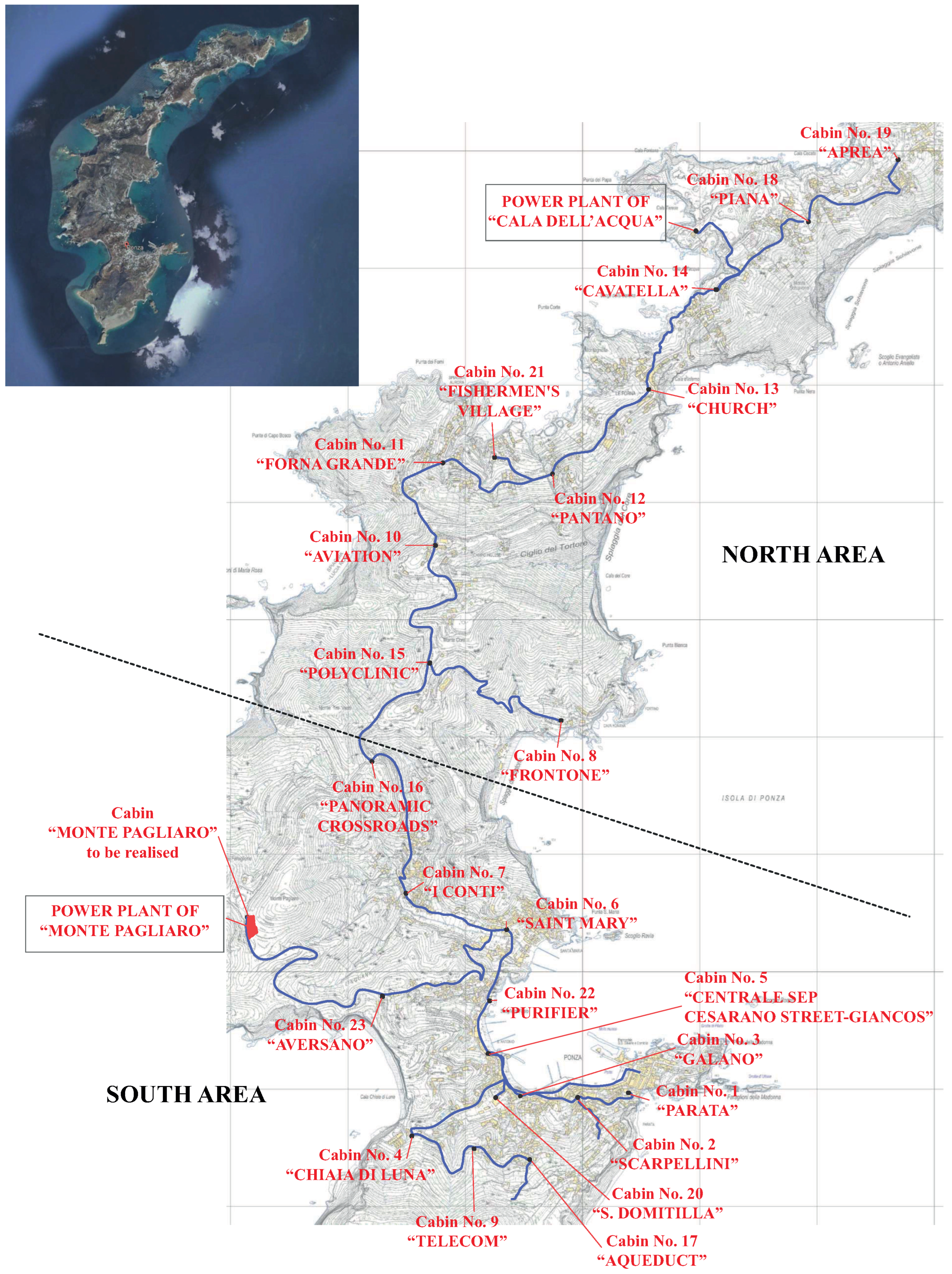
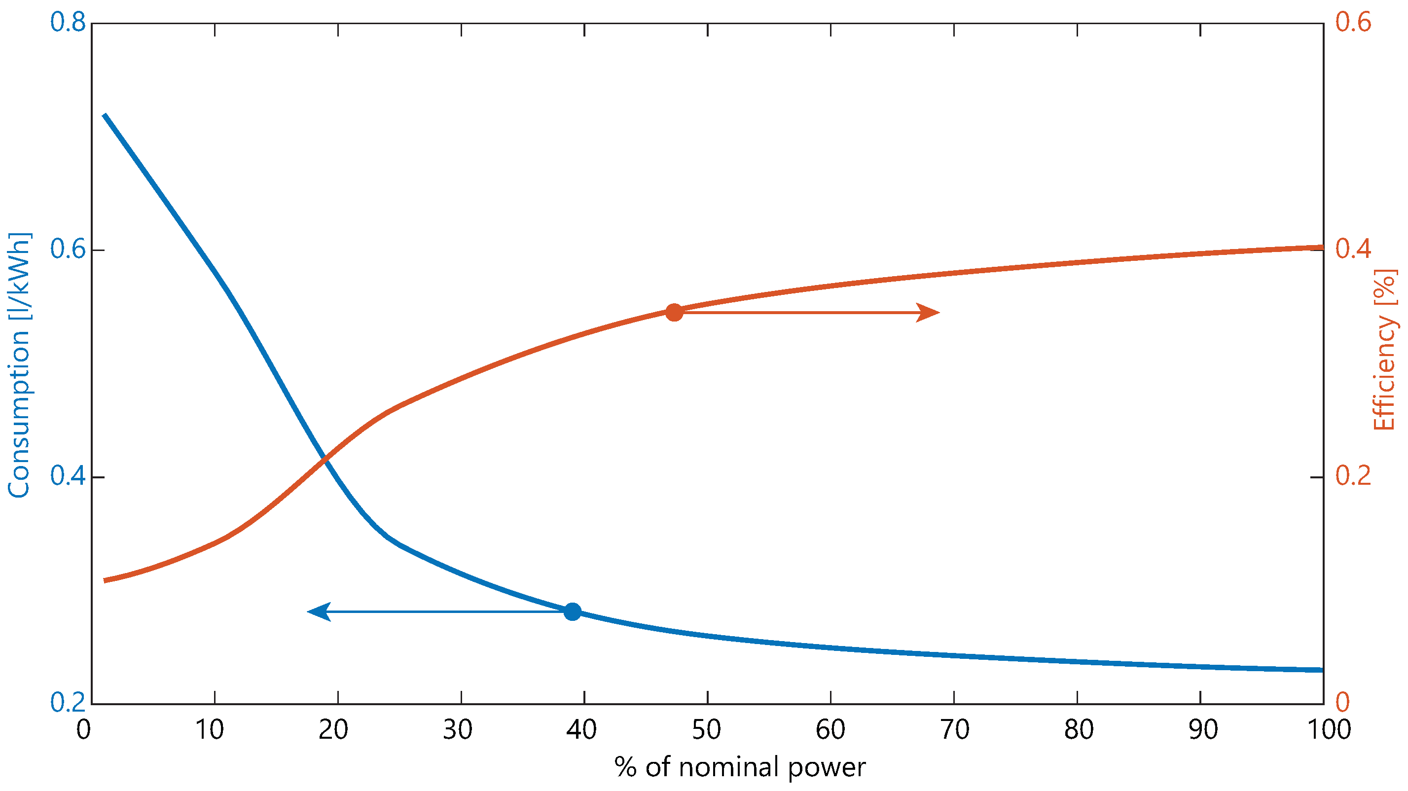
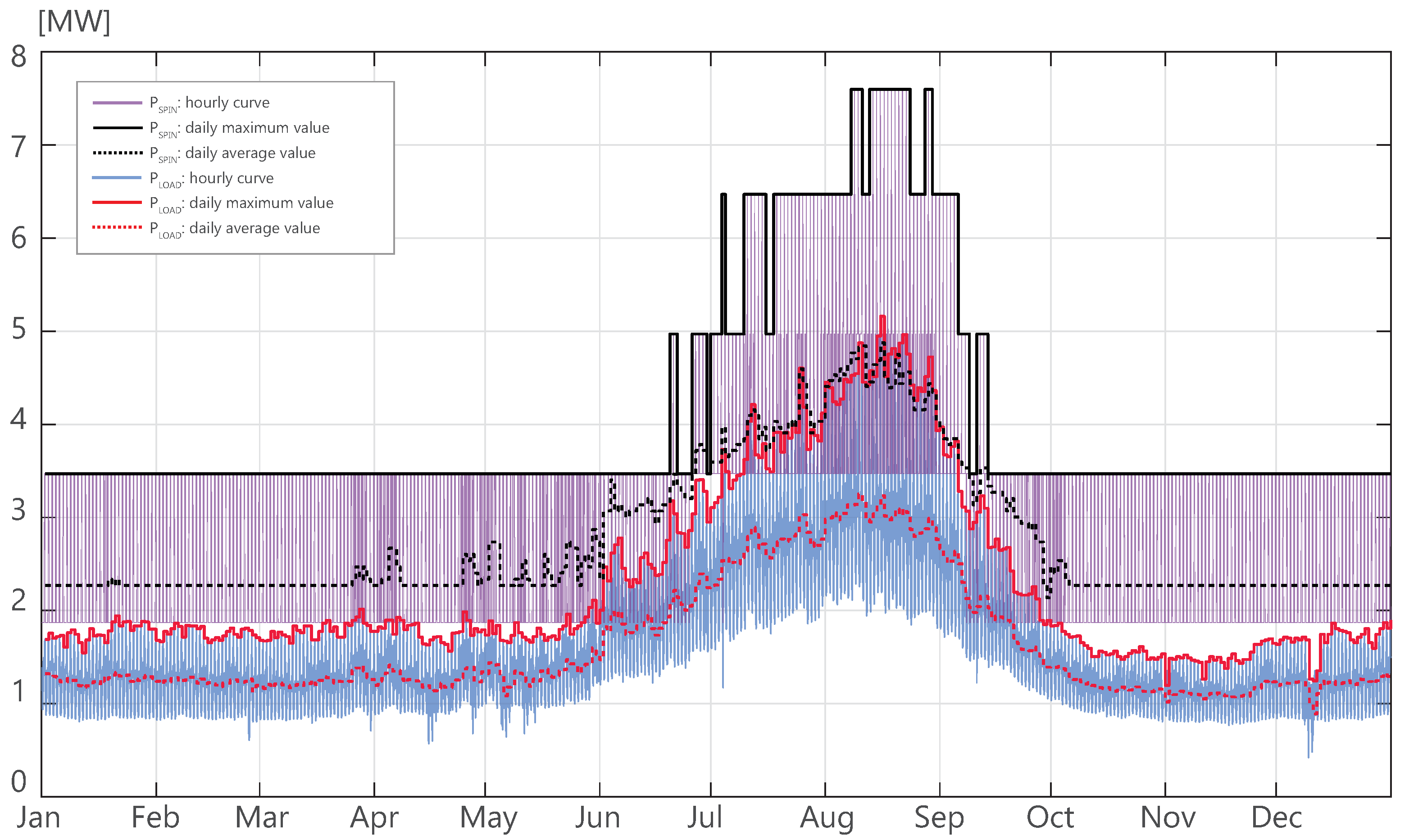
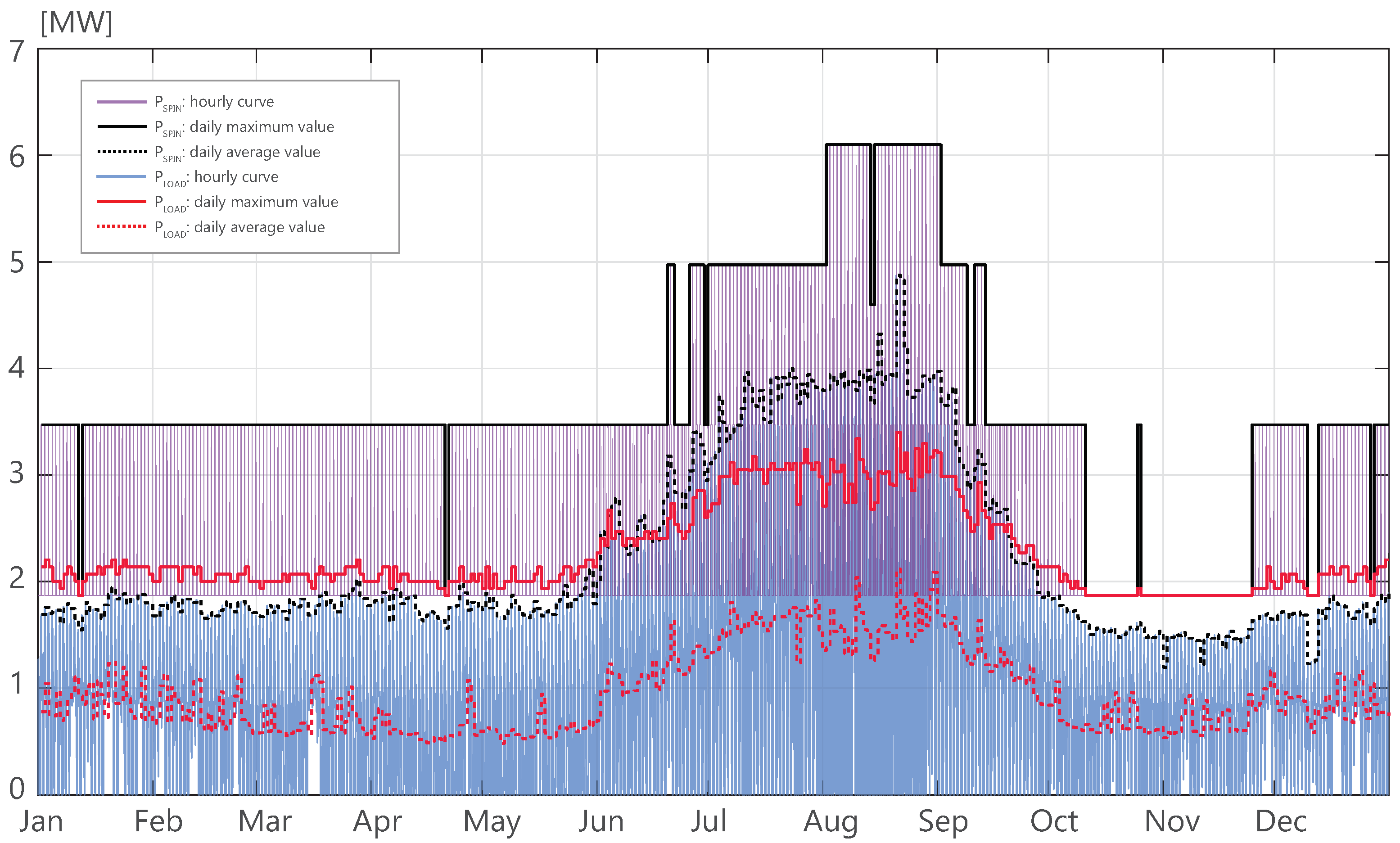
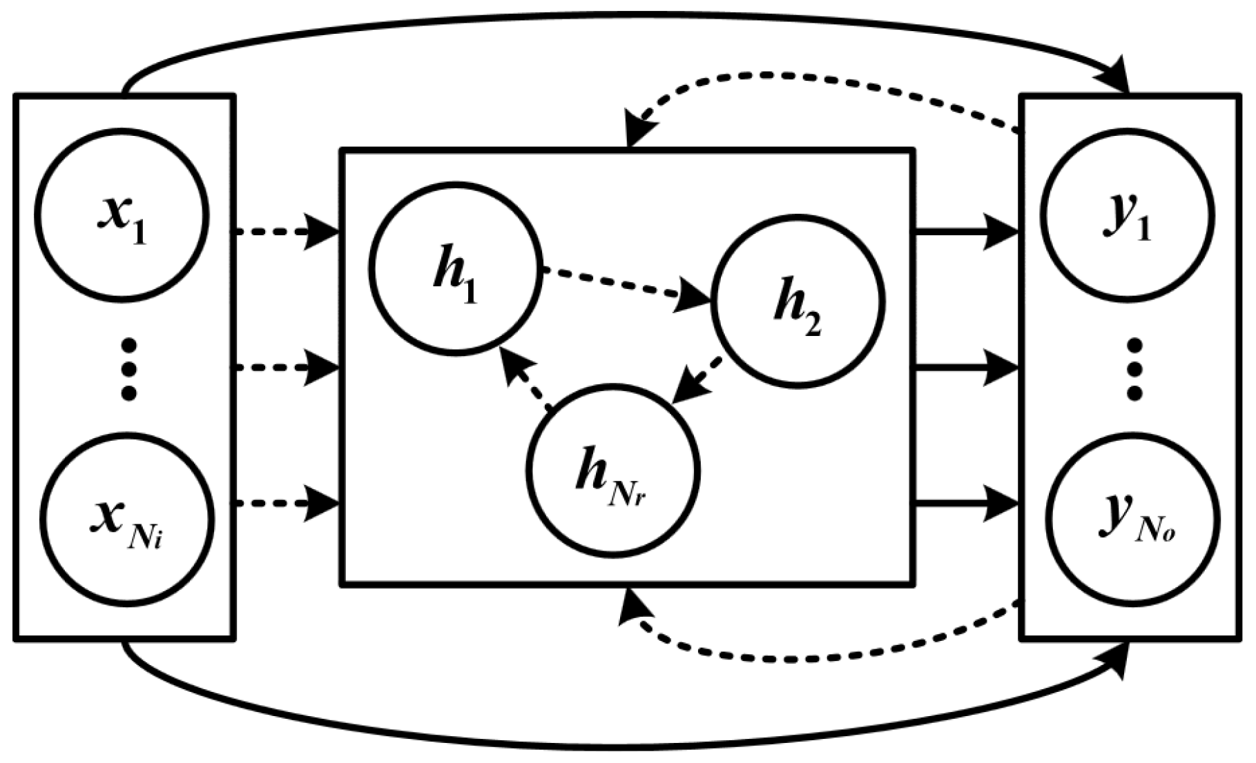
Table 1.
Electric load data of the island of Ponza.
| Total energy consumption | 11.792 in 2015 |
| 11.529 in 2016 | |
| Portion of load powered by Diesel generators | |
| Portion of load powered by RESs | |
| Maximum load | MW |
| Minimum load | MW |
| Average load | MW |
Table 2.
Control logic of diesel groups during summer.
| Generators | Time Slot | |
|---|---|---|
| Gen. 1 | Always running | Always running |
| Gen. 2 | In function if kW | In function if kW |
| Gen. 3 | Turned off | In function if kW |
| Gen. 4 | In function if kW | In function if kW |
| Gen. 5 | Turned off | In function if kW |
Table 3.
Control logic of diesel groups for the rest of the year.
| Generators | Time Slot | ||
|---|---|---|---|
| Gen. 1 | Always running | Always running | Always running |
| Gen. 2 | Turned off | In function if kW | Always running |
| Gen. 3 | Turned off | Turned off | Turned off |
| Gen. 4 | Turned off | Turned off | Turned off |
| Gen. 5 | Turned off | Turned off | Turned off |
Table 4.
Average values of efficiency and consumption of generators.
[%] | Efficiency [%] | Consumption | |
|---|---|---|---|
| [g/kWh] | [l/kWh] | ||
| 1 | 603 | ||
| 10 | 485 | ||
| 25 | 285 | ||
| 50 | 218 | ||
| 75 | 201 | ||
| 100 | 192 | ||
Table 5.
Annual operating data of the generators on the typical year (average of the years 2015 and 2016).
Table 5.
Annual operating data of the generators on the typical year (average of the years 2015 and 2016).
| Generators | Number of Power on | Hours of Operation [h] | Energy Produced [MWh] | Average Power [kW] | Average Load [%] | Average Efficiency [%] | Yearly Consumption [Ml] | Average Consumption | |
|---|---|---|---|---|---|---|---|---|---|
| [l/kWh] | [g/kWh] | ||||||||
| Gen. 1 | 1 | 8760 | 7786 | 889 | 231 | ||||
| Gen. 2 | 314 | 4221 | 3324 | 787 | 234 | ||||
| Gen. 3 | 76 | 403 | 355 | 878 | 227 | ||||
| Gen. 4 | 90 | 278 | 168 | 605 | 227 | ||||
| Gen. 5 | 25 | 45 | 28 | 624 | 230 | ||||
Table 6.
Simplified energy balance (average of the years 2015 and 2016).
| Description | Electricity [toe] | LPG [toe] | Petroleum Products [toe] |
|---|---|---|---|
| Input transformation | |||
| Power plants for thermoelectric generation | − | − | |
| Transformation output | |||
| Power plants for thermoelectric generation | − | − | |
| Consumption of energy sectors | |||
| Self-consumption of electricity generation | − | − | |
| Distribution losses | − | − | |
| Availability for final consumption | − | − | |
| Final energy consumption | |||
| Industry | − | ||
| Tertiary | − | ||
| Residential | − | ||
| Road transport | − | − | |
| Gross domestic consumption | |||
| Gross domestic consumption | |||
Table 7.
Energy demand by area (average of the years 2015 and 2016).
| Area | South Area | North Area |
|---|---|---|
| Electric demand [toe] | ||
| Electric demand [MWh] | 7909 | 3390 |
Table 8.
Electricity generation scenarios from RESs (energy and power).
| Decree Objectives 100% | Decree Objectives 300% | |||
|---|---|---|---|---|
| [MWh] | [MW] | [MWh] | [MW] | |
| PV | 903 | 1643 | ||
| Wind power | − | − | 1890 | |
| Cogeneration (ORC) | 240 | 240 | ||
| Total RESs | 1143 | 3773 | ||
Table 9.
Electric power from RES [kWe] according to the objectives of the Decree.
| Objective 100% | Objective 300% | |||
|---|---|---|---|---|
| South Area | North Area | South Area | North Area | |
| PV | 514 | − | 514 | 522 |
| Wind power | − | − | − | 900 |
| Cogeneration (ORC) | 100 | − | 100 | − |
| Total | 614 | − | 1514 | 522 |
Table 10.
BESSs deemed necessary to meet the objectives of the Decree.
| Decree Objectives 100% | Decree Objectives 300% | |||
|---|---|---|---|---|
| [MWh] | [MW] | [MWh] | [MW] | |
| South area “Ponza” | ||||
| North area “Le Forna” | − | − | ||
| Total | ||||
Table 11.
Estimated energy demand for 2030 (final consumption).
| Description | Electricity [toe] | LPG [toe] | Petroleum Products [toe] |
|---|---|---|---|
| Industry | − | ||
| Tertiary | − | ||
| Residential | − | ||
| Transportation | − | ||
| Total |
Table 12.
Estimated energy demand by area for 2030.
| Area | South Area | North Area |
|---|---|---|
| Electric demand [toe] | 700 | 522 |
| Electric demand [MWh] | 8141 | 6070 |
Table 13.
Evolution of diesel generators to 2030.
| Today | 2030 | |||
|---|---|---|---|---|
| Generator | Power | Typology | Power | Typology |
| [kW] | [kW] | |||
| Power plant of Monte Pagliaro | ||||
| Gen. 1 | 1600 | DEUTZ DZ 2046 | 1600 | DEUTZ DZ 2046 |
| Gen. 2 | 1500 | DEUTZ 620 | 1500 | DEUTZ 620 |
| Gen. 3 | 1500 | CAT 3516I | 1500 | CAT 3516I |
| Gen. 4 | 1020 | CAT 3512 | 1870 | CAT 3516 BHDTA |
| Gen. 5 | − | − | 1870 | CAT 3516 BHDTA |
| Power plant of Cala dell’Acqua | ||||
| Gen. 6 | 1128 | CAT 3516 HDTA | 1128 | CAT 3516 HDTA |
| Gen. 7 | 1128 | CAT 3516 HDTA | 1128 | CAT 3516 HDTA |
Table 14.
Control logic of diesel groups in August.
| Current Generators | Time Slot 0−24 |
|---|---|
| Gen. 1 | Always running |
| Gen. 2 | In function if kW |
| Gen. 6 | In function if kW |
| Gen. 4 | In function if kW |
Table 15.
Control logic of diesel groups in the rest of the year.
| Current Generators | Time Slot 0−24 |
|---|---|
| Gen. 1 | Always running |
| Gen. 2 | In function if kW |
| Gen. 6 | In function if kW |
| Gen. 4 | In function if kW |
Table 16.
Annual operating data of the generators on the typical year with BESS envisaged by 100% objectives of the Decree.
Table 16.
Annual operating data of the generators on the typical year with BESS envisaged by 100% objectives of the Decree.
| Generators | Number of Power on | Hours of Operation | Energy Produced | Average Power | Average Load | Average Efficiency | Yearly Consumption | Average Consumption | |
|---|---|---|---|---|---|---|---|---|---|
| [h] | [MWh] | [kW] | [%] | [%] | [Ml] | [l/kWh] | [g/kWh] | ||
| Gen. 1 | 1 | 8760 | 8808 | 1005 | 224 | ||||
| Gen. 2 | 220 | 2707 | 2556 | 944 | 224 | ||||
| Gen. 3 | 35 | 123 | 119 | 969 | 223 | ||||
| Gen. 4 | 21 | 34 | 26 | 737 | 219 | ||||
| Gen. 6 | 38 | 184 | 152 | 827 | 218 | ||||
Table 17.
Annual operating data of the generators on the typical year with BESS and RES envisaged by the 100% objectives of the Decree.
Table 17.
Annual operating data of the generators on the typical year with BESS and RES envisaged by the 100% objectives of the Decree.
| Generators | Number of Power on | Hours of Operation | Energy Produced | Average Power | Average Load | Average Efficiency | Yearly Consumption | Average Consumption | |
|---|---|---|---|---|---|---|---|---|---|
| [h] | [MWh] | [kW] | [%] | [%] | [Ml] | [l/kWh] | [g/kWh] | ||
| Gen. 1 | 1 | 8760 | 8117 | 927 | 229 | ||||
| Gen. 2 | 250 | 2321 | 2112 | 910 | 226 | ||||
| Gen. 3 | 35 | 123 | 119 | 969 | 223 | ||||
| Gen. 4 | 21 | 34 | 25 | 737 | 219 | ||||
| Gen. 6 | 32 | 175 | 145 | 831 | 218 | ||||
Table 18.
Possible control logic of diesel groups by 2030: Summer.
| Generators to 2030 | Time Slot | |
|---|---|---|
| Gen. 4 | Always running | Always running |
| Gen. 1 | In function if kW | In function if kW |
| Gen. 2 | Turned off | In function if kW |
| Gen. 3 | In function if kW | In function if kW |
| Gen. 6 | Turned off | In function if kW |
Table 19.
Possible control logic of diesel groups by 2030: rest of the year.
| Generators to 2030 | Time Slot | ||
|---|---|---|---|
| Gen. 1 | Always running | Always running | Always running |
| Gen. 2 | Turned off | In function if kW | Always running |
| Gen. 3 | Turned off | Turned off | Turned off |
| Gen. 4 | Turned off | Turned off | Turned off |
| Gen. 5 | Turned off | Turned off | Turned off |
Table 20.
Forecast of the annual operating data of the generators to 2030 in a purely conventional production scenario.
Table 20.
Forecast of the annual operating data of the generators to 2030 in a purely conventional production scenario.
| Generators | Number of Power on | Hours of Operation | Energy Produced | Average Power | Average Load | Average Efficiency | Yearly Consumption | Average Consumption | |
|---|---|---|---|---|---|---|---|---|---|
| [h] | [MWh] | [kW] | [%] | [%] | [Ml] | [l/kWh] | [g/kWh] | ||
| Gen. 4 | 1 | 8760 | 9751 | 1113 | 228 | ||||
| Gen. 1 | 342 | 4340 | 3966 | 914 | 230 | ||||
| Gen. 2 | 81 | 452 | 433 | 958 | 224 | ||||
| Gen. 3 | 113 | 425 | 398 | 937 | 225 | ||||
| Gen. 5 | 21 | 34 | 24 | 704 | 225 | ||||
Table 21.
Possible control logic of diesel groups by 2030 with RESs and BESSs: Summer.
| Generators to 2030 | Time Slot 0−24 |
|---|---|
| Gen. 4 | Always running |
| Gen. 1 | In function if kW |
| Gen. 6 | In function if kW |
| Gen. 4 | In function if kW |
Table 22.
Possible Control Logic of Diesel Groups by 2030 with RESs and BESSs: Rest of the Year.
| Generators to 2030 | Time Slot 0−24 |
|---|---|
| Gen. 4 | Always running |
| Gen. 1 | In function if kW |
| Gen. 2 | In function if kW |
| Gen. 3 | In function if kW |
Table 23.
Forecast of the annual operating data of the generators to 2030 with the integration of BESSs and RESs to 300% of the objectives of the Decree.
Table 23.
Forecast of the annual operating data of the generators to 2030 with the integration of BESSs and RESs to 300% of the objectives of the Decree.
| Generators | Number of Power on | Hours of Operation | Energy Produced | Average Power | Average Load | Average Efficiency | Yearly Consumption | Average Consumption | |
|---|---|---|---|---|---|---|---|---|---|
| [h] | [MWh] | [kW] | [%] | [%] | [Ml] | [l/kWh] | [g/kWh] | ||
| Gen. 4 | 1 | 8760 | 6805 | 777 | 227 | ||||
| Gen. 1 | 414 | 2937 | 2980 | 1015 | 224 | ||||
| Gen. 2 | 83 | 466 | 492 | 1056 | 220 | ||||
| Gen. 3 | 103 | 287 | 312 | 1087 | 219 | ||||
| Gen. 5 | 65 | 253 | 210 | 830 | 218 | ||||
Table 24.
Forecast of the annual operating data of the generators to 2030 with the integration of BESS and RES to 100% of the objectives of the Decree.
Table 24.
Forecast of the annual operating data of the generators to 2030 with the integration of BESS and RES to 100% of the objectives of the Decree.
| Generators | Number of Power on | Hours of Operation | Energy Produced | Average Power | Average Load | Average Efficiency | Yearly Consumption | Average Consumption | |
|---|---|---|---|---|---|---|---|---|---|
| [h] | [MWh] | [kW] | [%] | [%] | [Ml] | [l/kWh] | [g/kWh] | ||
| Gen. 4 | 1 | 8760 | 9835 | 1123 | 227 | ||||
| Gen. 1 | 281 | 3027 | 2989 | 987 | 225 | ||||
| Gen. 2 | 48 | 235 | 246 | 1045 | 220 | ||||
| Gen. 3 | 32 | 168 | 168 | 1003 | 222 | ||||
| Gen. 5 | 35 | 247 | 190 | 770 | 261 | ||||
Table 25.
Unit costs for plants.
| Name | Cost |
|---|---|
| Underground cable line Al 185 on natural ground | 63 k€/km |
| Underground cable line Al 185 on asphalted road with fillings and with | 150 k€/km |
| mixed cement and repairs | |
| Network insertion joints for delivery cabin connection solution with in-out in | 2.5 k€ |
| underground cable | |
| Sectioning cabin (cabin building) inserted on an underground cable line | 11 k€ |
| Outfitting of in-out delivery cabin (excluding cabin artifact) | 7.5 k€ |
| Shunt delivery cabin set-up | 5.5 k€ |
| Disconnection device in the existing secondary cabin/substation (with space | 3.5 k€ |
| available for an additional compartment) | |
| PV plant | 0.9 k€/kWp |
| Wind power plant | 1.15 k€/kW |
| BESS | 350 k€/MW |
| BESS | 0.33 k€/kWh |
| Cogeneration | 2 k€/kW |
| Smart meters | 2.5 k€/kW |
| Control center | 10 k€/kW |
Table 26.
Sources of financing/co-financing.
| References | Object and Conditions | Maximum Amount of Financing | Expected Amount of Financing | Interest Rate |
|---|---|---|---|---|
| NATIONAL: | ||||
| Nuova Sabatini | Machinery, hardware systems, software, digital technologies for small and medium-sized enterprises | 2 M€ | 1.4 M€ | 2.75% |
| MCC SPA Fund | Productive investments for small and medium-sized enterprises | 2.5 M€ | 1.668 M€ | Facilitated according to company rating |
| REGIONAL: | ||||
| APEA Lazio Region | Reduction of energy consumption and emissions for micro and large enterprises | 200 k€ | 200 k€ | Non-repayable loan of 50% |
Disclaimer/Publisher’s Note: The statements, opinions and data contained in all publications are solely those of the individual author(s) and contributor(s) and not of MDPI and/or the editor(s). MDPI and/or the editor(s) disclaim responsibility for any injury to people or property resulting from any ideas, methods, instructions or products referred to in the content. |
© 2023 by the authors. Licensee MDPI, Basel, Switzerland. This article is an open access article distributed under the terms and conditions of the Creative Commons Attribution (CC BY) license (https://creativecommons.org/licenses/by/4.0/).
Share and Cite
MDPI and ACS Style
Succetti, F.; Rosato, A.; Araneo, R.; Di Lorenzo, G.; Panella, M. Challenges and Perspectives of Smart Grid Systems in Islands: A Real Case Study. Energies 2023, 16, 583. https://0-doi-org.brum.beds.ac.uk/10.3390/en16020583
AMA Style
Succetti F, Rosato A, Araneo R, Di Lorenzo G, Panella M. Challenges and Perspectives of Smart Grid Systems in Islands: A Real Case Study. Energies. 2023; 16(2):583. https://0-doi-org.brum.beds.ac.uk/10.3390/en16020583
Chicago/Turabian StyleSuccetti, Federico, Antonello Rosato, Rodolfo Araneo, Gianfranco Di Lorenzo, and Massimo Panella. 2023. "Challenges and Perspectives of Smart Grid Systems in Islands: A Real Case Study" Energies 16, no. 2: 583. https://0-doi-org.brum.beds.ac.uk/10.3390/en16020583
Note that from the first issue of 2016, this journal uses article numbers instead of page numbers. See further details here.