Design of Thermoelectric Generators and Maximum Electrical Power Using Reduced Variables and Machine Learning Approaches

Abstract

This work aims to contribute to studies on the geometric optimization of thermoelectric generators $\left(TEGs\right)$ through a combination of the reduced variables technique and supervised machine learning. The architecture of the thermoelectric generators studied, one conventional and the other segmented, was determined by calculating the cross-sectional area and length of the legs, and applying reduced variables approximation. With the help of a supervised machine learning algorithm, the values of the thermoelectric properties were predicted, as were those of the maximum electrical power for the other temperature values. This characteristic was an advantage that allowed us to obtain approximate results for the electrical power, adjusting the design of the $TEGs$ when experimental values were not known. The proposed method also made it possible to determine the optimal values of various parameters of the legs, which were the ratio of the cross-sectional areas $(A_p/A_n)$, the length of the legs $\left(l\right)$, and the space between the legs $\left(H\right)$. Aspects such as temperature-dependent thermoelectric properties (Seebeck coefficient, electrical resistivity, and thermal conductivity) and the metallic bridge that connects the legs were considered in the calculations for the design of the $TEGs$, obtaining more realistic models. In the training phase, the algorithm received the parameter $\left(H\right)$ and an operating temperature value as input data, to predict the corresponding value of the maximum power produced. This calculation was performed for conventional and segmented systems. Recent advances have opened up the possibility of applying an algorithm for designing conventional and segmented thermocouples based on the reduced variables approach and incorporating a supervised machine learning computational technique.

1. Introduction

The design of thermoelectric generators $\left(TEGs\right)$ using geometric optimization techniques is the topic of interest in this work. Here, we describe some advantages of this type of design. First, it allows us to make better use of the thermoelectric material; to date, the best materials have been inorganic compounds (such as $B{i}_{2}T{e}_3$), which have a relatively low abundance on Earth, and their manufacture requires a highly complex vacuum process. It is also possible to gradually adjust the dimensions of the system according to the space available for its coupling to a heat source. One parameter used in the geometric method is the cross-sectional area of the leg [1]. For example, it is possible to maximize the output power of the $TEG$ as a function of the variable cross-section; in fact, in [2], it was stated that “The geometry of the $TEG$ has a vital impact on the thermal resistance and the electrical resistance, influencing its integral performance”.

Another aspect that motivated the development of this work is the emergence of new manufacturing techniques, such as additive manufacturing, which allow customizing thermoelectric systems according to the requirements of the field of application (from low-power applications, medical and wearable devices, Internet of Things, and wireless sensor networks; to high-power applications, industrial electronics, automotive engines, and aerospace). However, as rightly mentioned in [3], “little knowledge exists about which shapes are beneficial in applications with different thermal conditions”. This author analyzed the effect of different thermoelectric leg designs on device performance. The authors in [4] proposed an optimized design of legs with special geometric shapes and their manufacture using 3D printing to increase the output power of $TEGs$.

In [2], two relevant aspects were mentioned: (a) in the current literature, there are still few studies on the optimization of the geometry of $TEGs$, especially for the shape of the legs; (b) recently, algorithms have been used to design optimal devices by simultaneously analyzing two or more geometric parameters.

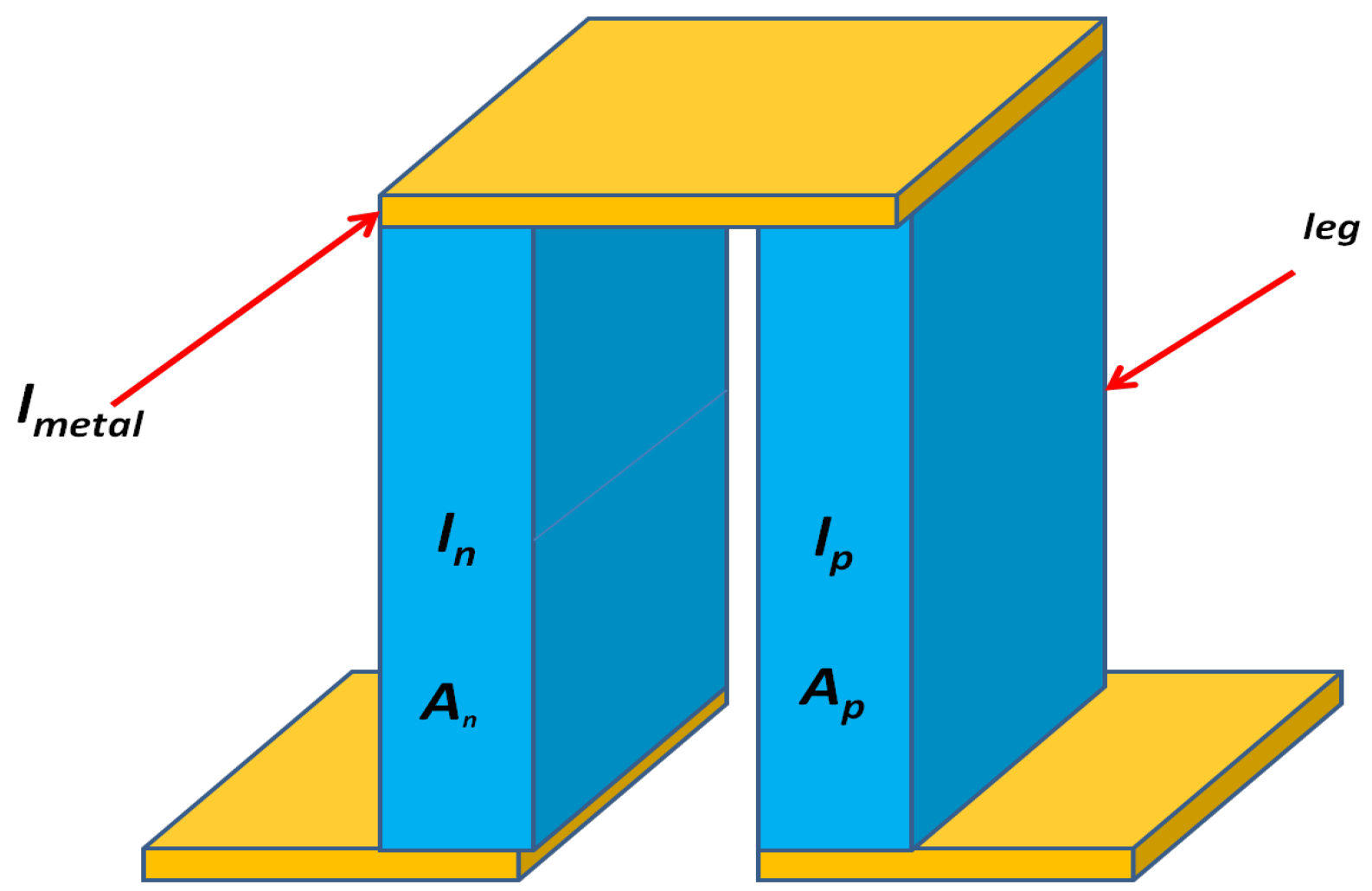
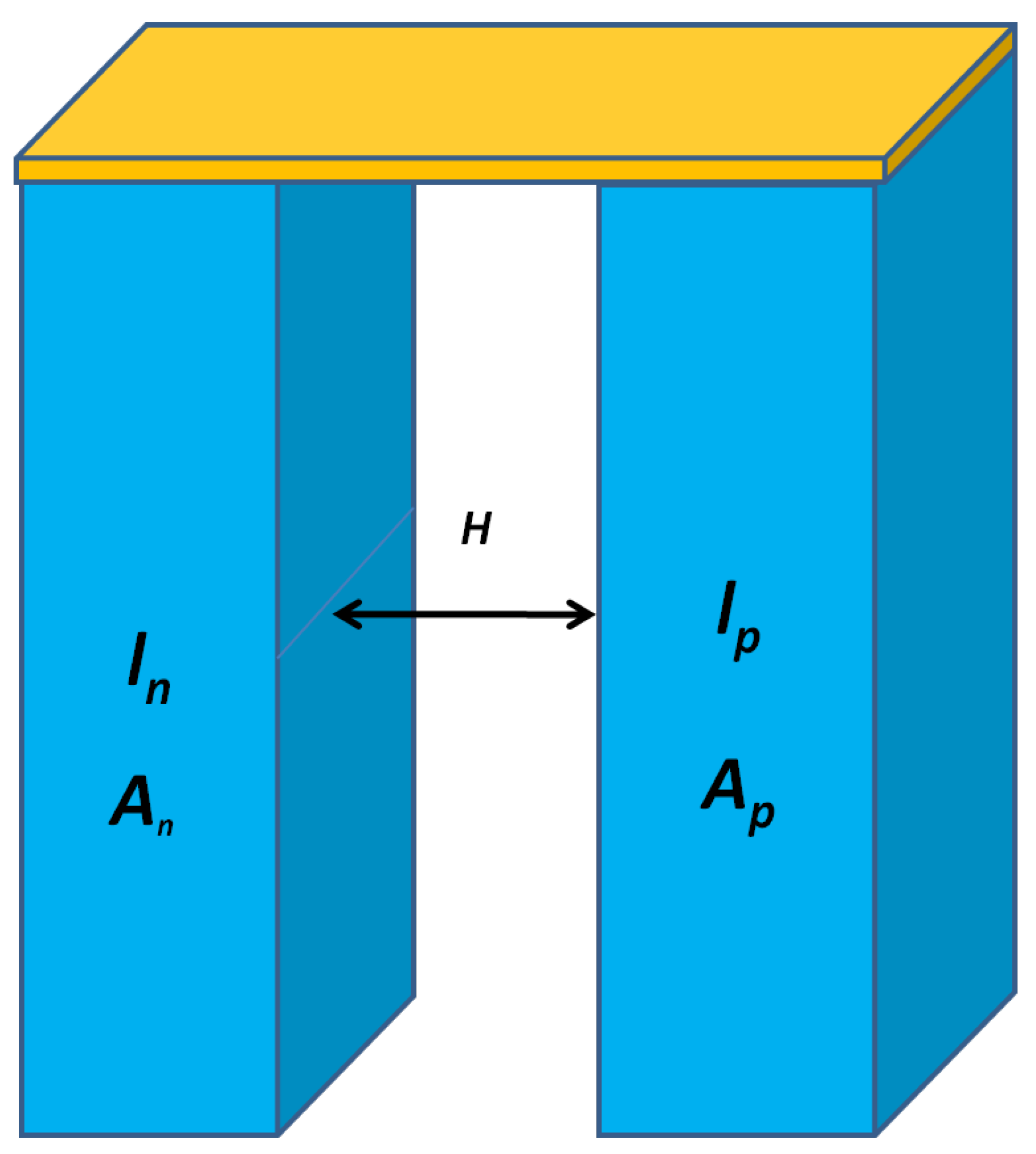
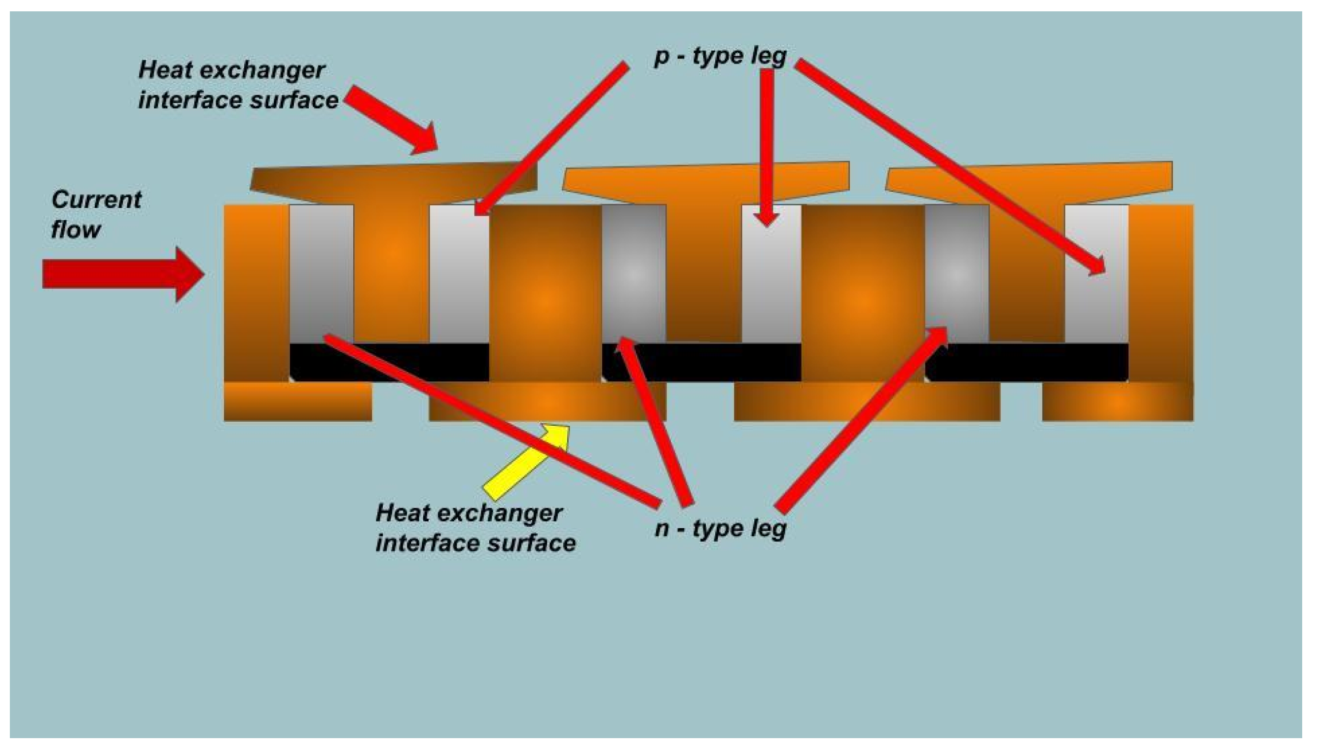
The idea of geometric optimization comes from the structural aspect of the thermoelectric generator, which in its most elementary form (thermocouple) is composed of two legs of semiconductor material (for example, BiTe or SiGe), one n-type and the other p-type, which are electrically connected in series by means of a metallic bridge (for example, copper) (Figure 1); these legs have a rectangular prism shape. Then, two geometric parameters present in each leg are identified, the cross-sectional area $\left(A\right)$ and the length $\left(l\right)$. These geometric parameters are linked to two properties of thermoelectric materials, thermal conductance (K) and electrical resistance (R). This relationship between the geometric parameters and the thermoelectric properties is useful for adjusting the shape and size of the thermocouple. To achieve this dimensioning, a useful technique is the analysis of the electrical power produced by the TEG, in terms of the geometric parameters.

The main motivation for carrying out this work arose from identifying that currently, in the thermoelectricity field, there is a growth in the amount of researchers interested in developing $TEGs$ devices for harvesting energy from waste heat sources [5,6]. To achieve the maximum use of this heat, it is essential to analyze the geometric characteristics of the device. As previously mentioned, geometric optimization methods require knowledge of thermoelectric properties, which are linked to the dimensional parameters and that also vary with temperature. These conditions require knowledge of property measurements to achieve the best adjusted $TEG$ design for the requirements imposed by the heat source, the available space, and the load resistance of the system that will use the power produced by the $TEGs$. However, not all researchers attempting to design $TEGs$ have a materials laboratory or the equipment required to prepare samples and measurements. At present, a useful resource is simulation software to study the properties of materials and design $TEGs$; even so, depending on the type of software, investment in licensing is required, in addition to high-end computer equipment.

Seeking to develop an affordable alternative for the community intending to design $TEGs$, in this work, we propose developing a methodology built on three principles:

(I) Use data from experimental measurements found in publications by specialists in thermoelectric materials; (II) Use a formalism or an approximation that allows the immediate use of the data obtained from the literature to obtain the leg dimensions $(An,Ap,l)$; (III) Merge the selected formalism or approximation with a prediction algorithm that allows us to generate the design best adjusted to the operating conditions of the environment.

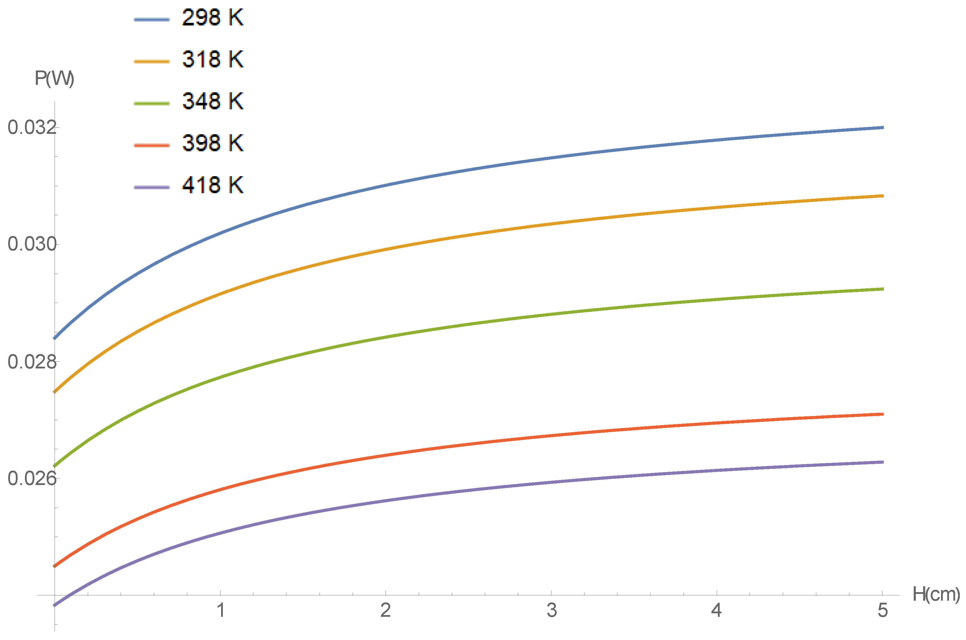
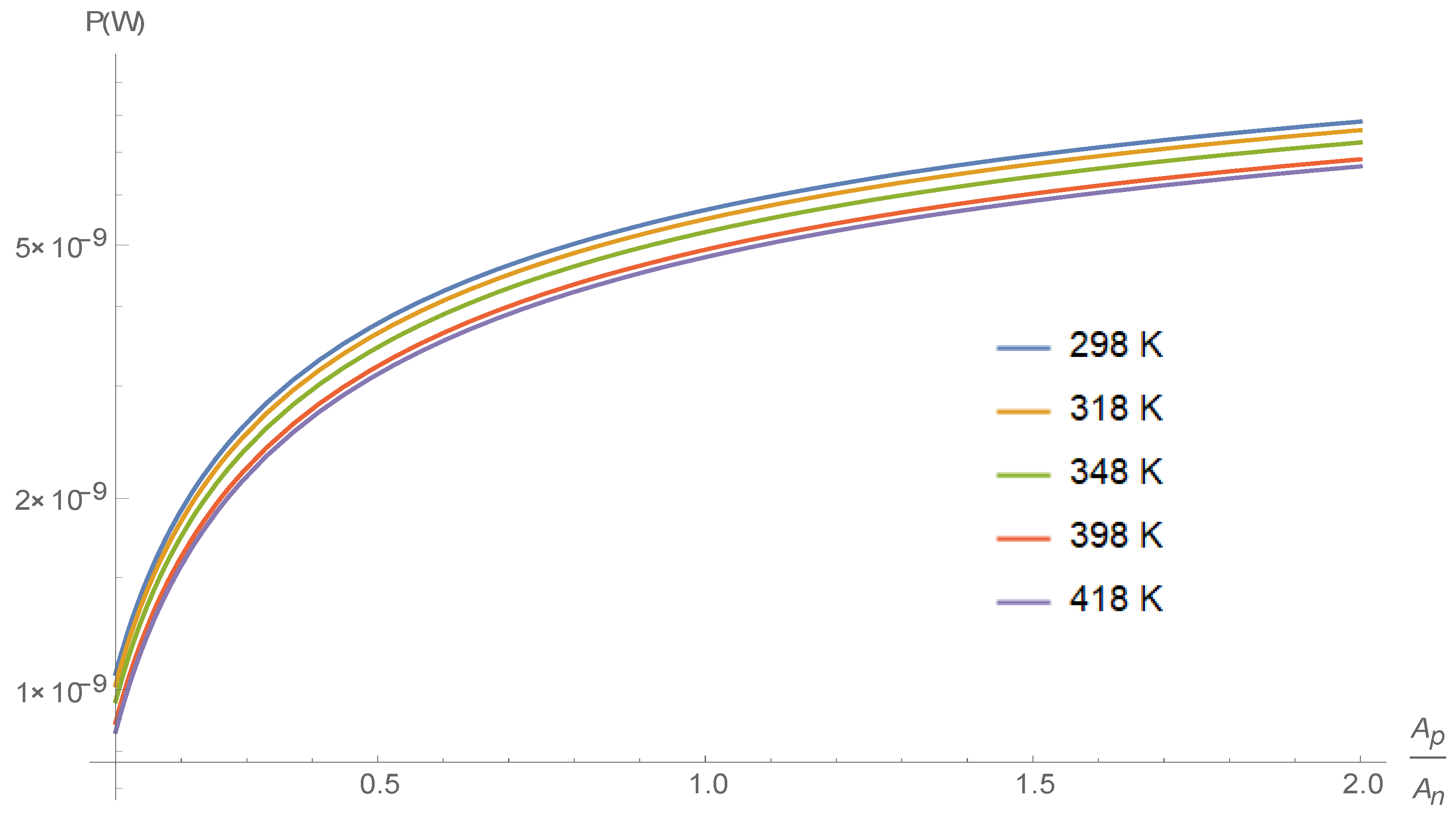
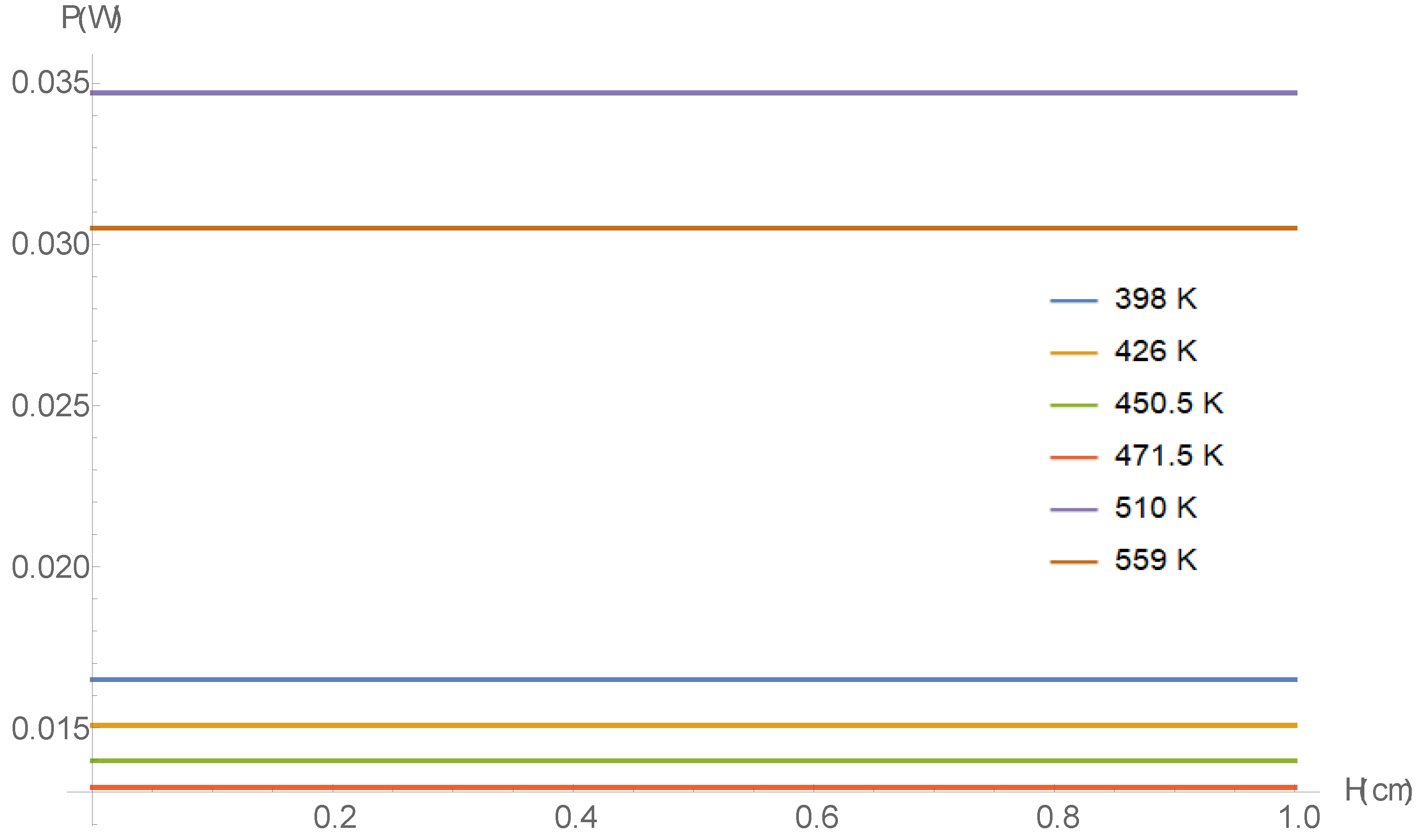
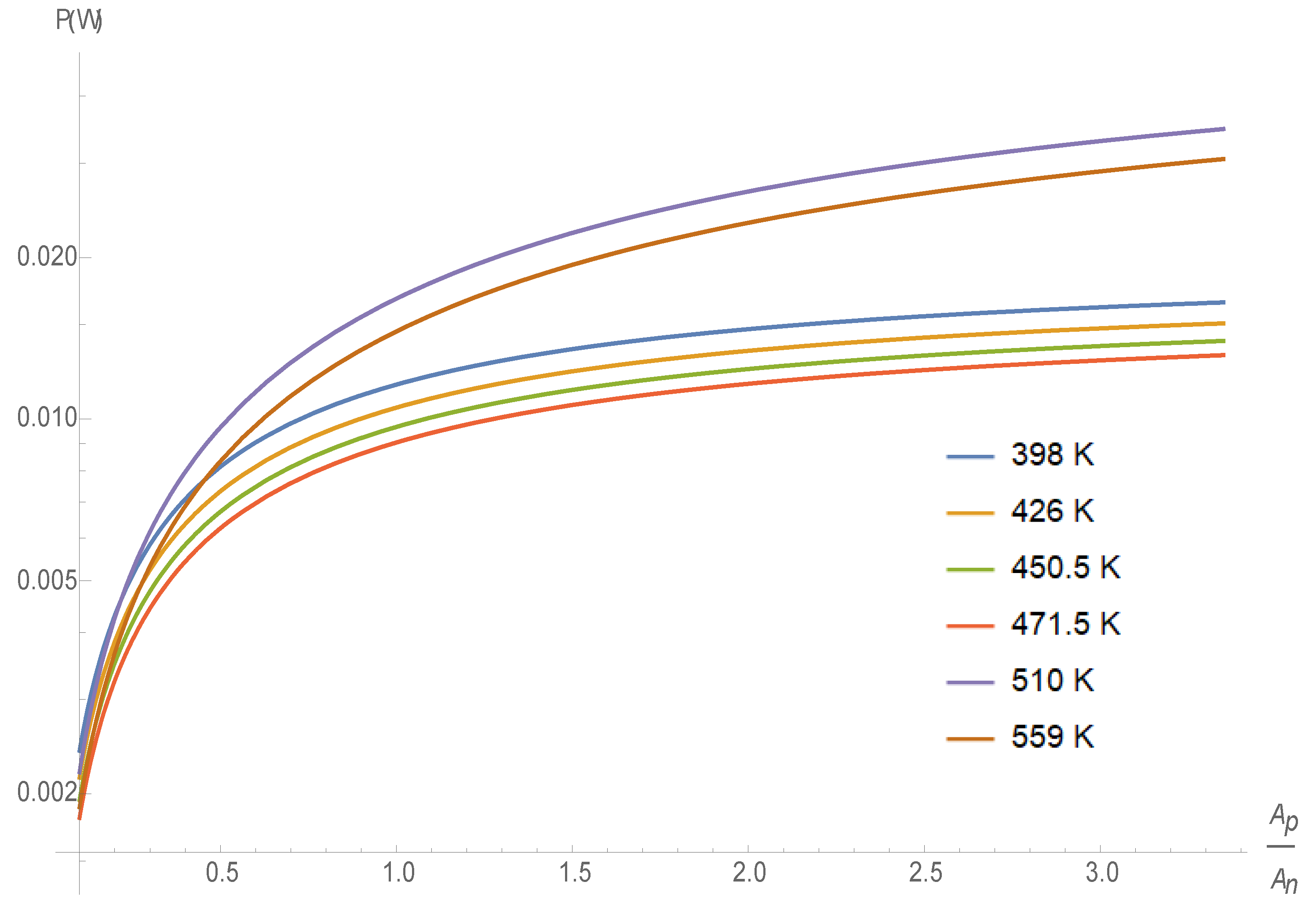
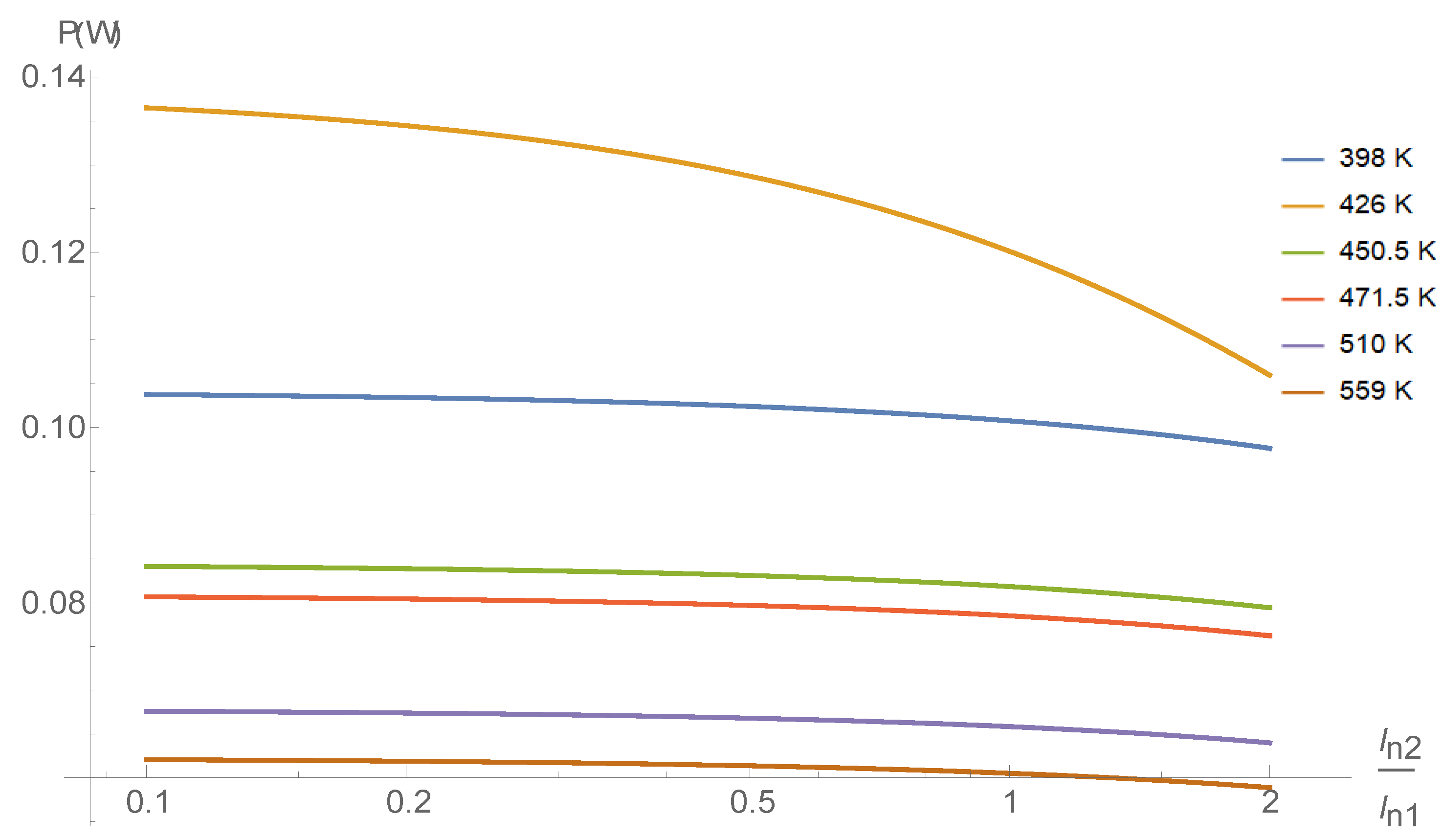
The three previous principles guided us toward combining the reduced variables technique with supervised machine learning $\left(SML\right)$ in a design process that consists of the following steps: (a) take advantage of the qualities of the reduced current approximation to obtain the architecture of the thermoelectric generator by calculating the parameters (cross-sectional area and length of its legs); (b) with the help of an algorithm $\left(SML\right)$, the values of the thermoelectric properties and the maximum electrical power $\left(P\right)$ are predicted for any temperature value; and (c) the values obtained in the prediction are useful for adjusting the design for the operating conditions. In addition, the algorithm has the outstanding feature of simultaneously analyzing and determining various parameters related to the geometry of the legs that maximize $\left(P\right)$. These parameters are the cross-sectional area ratio $(Ap/An)$, length $\left(l\right)$, length n ratio $(l{n}_2/l{n}_1)$, length p ratio $(l{p}_2/l{p}_1)$ (in the case of a segmented $TEG$), and the space between legs $\left(H\right)$.

The results provide useful information for the construction of optimal devices and their possible applications. The scope of this work was extended to a new training phase, in which it is possible to introduce values of the parameter H and of the temperature, managing to predict the corresponding value of the maximum power. Of course, this study has limitations, which are discussed in later sections; however, these first results allowed us to determine that it is possible to obtain an algorithm for the design of conventional and segmented thermocouples based on a reduced variables approach fused with a supervised machine learning calculation model, trained for various thermoelectric materials. The utility and scope of the method are shown when confronted with a computerized and experimental model in Section 6.

Notes on the State of the Art

The reduced variables approach is a strategy that can be applied for the optimization of power, efficiency, and even the coefficient of performance, modifying the current flow in the legs by adjusting the cross-sectional area. This feature allows us to model the architecture of the TEG, managing the size of the cross-sectional area and length of the legs. The scope of this tool was reported in the works of [7,8,9,10].

On the other hand, in the field of thermoelectricity, machine learning has been applied for the prediction of material properties and for the design of new materials. As [11] rightly mentioned, “the machine learning technique can provide a powerful discovery tool for thermoelectric materials with respect to the new chemical composition, nanostructural design, stoichiometry optimization, etc.”. Specifically, supervised machine learning, which is based on algorithms that learn from an input dataset and a training dataset and manage to predict unseen data or future values—divided into two categories of classification and regression [12]—has been applied to carry out the synthesis of a new material spin-driven thermoelectric effect (STE) [13].

2. Related Work

In the search for a sustainable society and world, thermoelectric generators are an alternative that can contribute to the economic and social development of regions where it is possible to take advantage of the products generated by biodiversity; for example, in [14], the coupling of a thermoelectric generator in a lignin biorefinery was reported (which is a heteropolymer that is part of the cell wall of the vascular tissue of plants, one of the main components of the biomass that can be used to obtain renewable products as raw material for biofuels). The use of thermoelectric generators for the recovery of waste heat from biomass stoves was reported in [15]; in this work, the voltage produced by a thermoelectric generator placed between the hot wall of a stove and a heatsink was investigated. The voltage produced by this system was measured and compared for different biomass fuels, such as wood chips, walnut shells, cobs of corn, and coconut shells. Their results showed that each biomass fuel had its own combustion characteristics that allowed the $TEG$ to generate a high voltage at specific values. It is also very interesting to comment on the work of [16], in which a self-powered marine mammal condition monitoring system was proposed based on the hybrid energy-harvesting mode of a triboelectric nanogenerator $\left(TENG\right)$ and a thermoelectric microgenerator $\left(MTEG\right)$.

Table 1. Related work.

Reference	Characteristics
[1]	A thermal-electric coupled mixed-method algorithm that predicts TEG performance and optimizes the crosssectional area along the leg length in order to optimize power output or thermal conversion efficiency
[2]	This work proposes an optimization study to maximize the output power of variable cross-section $TEGs$ for solar energy utilization by coupling finite element method (FEM) and optimization algorithm. Six geometric variables along with the external load resistance are optimized by genetic algorithm (GA) and particle swarm optimization (PSO).
[3]	Various leg shapes (rectangular prisms, prisms with interior hollows, trapezoids, hourglass, and Y-shape) were modeled numerically to determine their thermal and electrical performance under constant temperature and heat flux boundary conditions. Two thermoelectric materials, bismuth telluride and silicon germanium, were modeled to capture both low and high temperature application cases, respectively.
[4]	This work proposes a new geometric design concept to improve the output voltage and power of the TE legs in RTGs based on increasing side area to enhance heat dissipation caused by convective heat transfer and radiative heat transfer. Helix-shaped and spoke-shaped TE legs with different geometrical shapes are designed.

below shows some very interesting works on the design of $TEGs$ that are related to the one presented in this article.

3. Materials and Methods

3.1. Conventional Thermocouple

Dimensional Parameters

The parameters used for the design of thermoelectric legs were the cross-sectional area $\left(A_n\right)$, $\left(A_p\right)$ and the length $(l_p=l_n=l)$. Snyder [10] rigorously formulated the reduced variable approximation. A critical parameter of this approximation is the reduced (relative) current, defined as:

$$u=\frac{J}{\kappa \nabla T}$$

(1)

where $\kappa$ is the thermal conductivity and T is the absolute temperature.

Snyder [10] proposed an iteration equation to calculate the numerical values of the quantity $\left(u\kappa \right)$ required for calculations. The $\left(u\kappa \right)$ values were obtained from tables consulted in [10] for different temperature values. This quantity is the kernel of the integrals that appear in Equations (4) and (12), which were used to calculate the cross-sectional area and length of the legs. Below is the detailed procedure for calculating $\left(A_n\right)$, $\left(A_p\right)$, and $\left(l\right)$, applying reduced variable approximation, which are the main parameters for $TEG$ design.

The first step in the reduced variable procedure is to establish the equal lengths of both legs; that is, $(l_p=l_n)$:

$$I=J_p{A}_p=J_n{A}_n$$

(2)

if the current density $\left(J\right)$ is defined as follows:

$$Jl={\int }_{T_c}^{T_h}\kappa udT$$

(3)

where $\kappa$ is the thermal conductance and u is the reduced current density. For a complete understanding of the equations of the reduced variable formalism used in this article, we suggest consulting reference [10]. Combining Equations (2) and (3), the following relationship is obtained:

$$\frac{A_p}{A_n}=\frac{-J_n}{J_p}=\frac{-{\int }_{T_c}^{T_h}{u}_n{\kappa }_{n}dT}{{\int }_{T_c}^{T_h}{u}_p{\kappa }_{p}dT}$$

(4)

To calculate the integrals of Equation (4), data from

Table 2. Numerical data $\left(u\kappa \right)$, material ($B{i}_{2}T{e}_3$).

T (K)	${\mathit{u}}_{\mathit{p}}{\mathit{k}}_{\mathit{p}}\mathit{d}\mathit{T}$ (A/cm)	${\mathit{u}}_{\mathit{n}}{\mathit{k}}_{\mathit{n}}\mathit{d}\mathit{T}$ (A/cm)
$T_0=298$	$u_p{k}_p\left(T_0\right)=0.8132$	$u_n{k}_n\left(T_0\right)=-0.4966$
$T_1=323$	$u_p{k}_p\left(T_1\right)=0.8350$	$u_n{k}_n\left(T_1\right)=-0.5206$
$T_2=348$	$u_p{k}_p\left(T_2\right)=0.8424$	$u_n{k}_n\left(T_2\right)=-0.5679$
$T_3=373$	$u_p{k}_p\left(T_3\right)=0.8435$	$u_n{k}_n\left(T_3\right)=-0.6312$
$T_4=398$	$u_p{k}_p\left(T_4\right)=0.8466$	$u_n{k}_n\left(T_4\right)=-0.6933$
$T_5=423$	$u_p{k}_p\left(T_5\right)=0.8603$	$u_n{k}_n\left(T_5\right)=-0.4454$

are required; these were obtained from the literature; see reference [10].

The integrals $-{\int }_{T_c}^{T_h}{u}_n{\kappa }_{n}dT$ and ${\int }_{T_c}^{T_h}{u}_p{\kappa }_{p}dT$ are calculated applying the Newton–Cotes method (fourth order). The results for each integral are shown:

$$-{\int }_{T_c}^{T_h}{u}_n{\kappa }_{n}dT=-57.78$$

(5)

$${\int }_{T_c}^{T_h}{u}_p{\kappa }_{p}dT=83.82$$

(6)

The area ratio is

$$\frac{A_p}{A_n}=0.69$$

(7)

Now, it is possible to calculate the current densities in the legs;

$$J_p=\frac{U_{total-h}}{A_{total}}\frac{1+\frac{A_n}{A_p}}{{\Phi }_{p-h}-{\Phi }_{n-h}}$$

(8)

${\Phi }_{p-h}$ and ${\Phi }_{n-h}$ are the thermoelectric potentials at temperature $T_h$ = 423 K;

$$\begin{array}{c}\hfill \frac{U_{total-h}}{A_{total}}=20(\mathrm{W}/{\mathrm{cm}}^2)\\ \hfill {\Phi }_{ph}=0.37\left(\mathrm{V}\right)\\ \hfill {\Phi }_{nh}=-0.49\left(\mathrm{V}\right)\end{array}$$

(9)

At these values, the current density in the p-type leg is

$$J_p=57.32\mathrm{mA}/{\mathrm{cm}}^2$$

(10)

For the current density in the n-type leg, the value $J_p$ and quotient (7) are used;

$$J_n=39.51\mathrm{mA}/{\mathrm{cm}}^2$$

(11)

Now, it is possible to know the length $\left(l\right)$, for which the following equation is applied:

$${\int }_{T_c}^{T_h}{k}_{n,p}{u}_{n,p}dT=J_{n,p}{l}_{n,p}$$

(12)

The next value of l is obtained;

$$\begin{array}{c}\hfill l=1.46\left(\mathrm{mm}\right)\end{array}$$

(13)

To calculate the cross-sectional areas $A_p$ and $A_n$, $A_{total}$ is defined as the total area. For calculation purposes, $A_{total}=1{\mathrm{mm}}^2$ is selected. The results are

$$\begin{array}{c}\hfill A_p=0.41{\mathrm{mm}}^2\\ \hfill A_n=0.59{\mathrm{mm}}^2\end{array}$$

(14)

Now, the thickness $\left(l_{metal}\right)$ of the metal bridge is added. Figure 1 shows a sketch of the design obtained:

This first system can be used as a basic unit for the design of a thermoelectric module composed of several thermocouples.

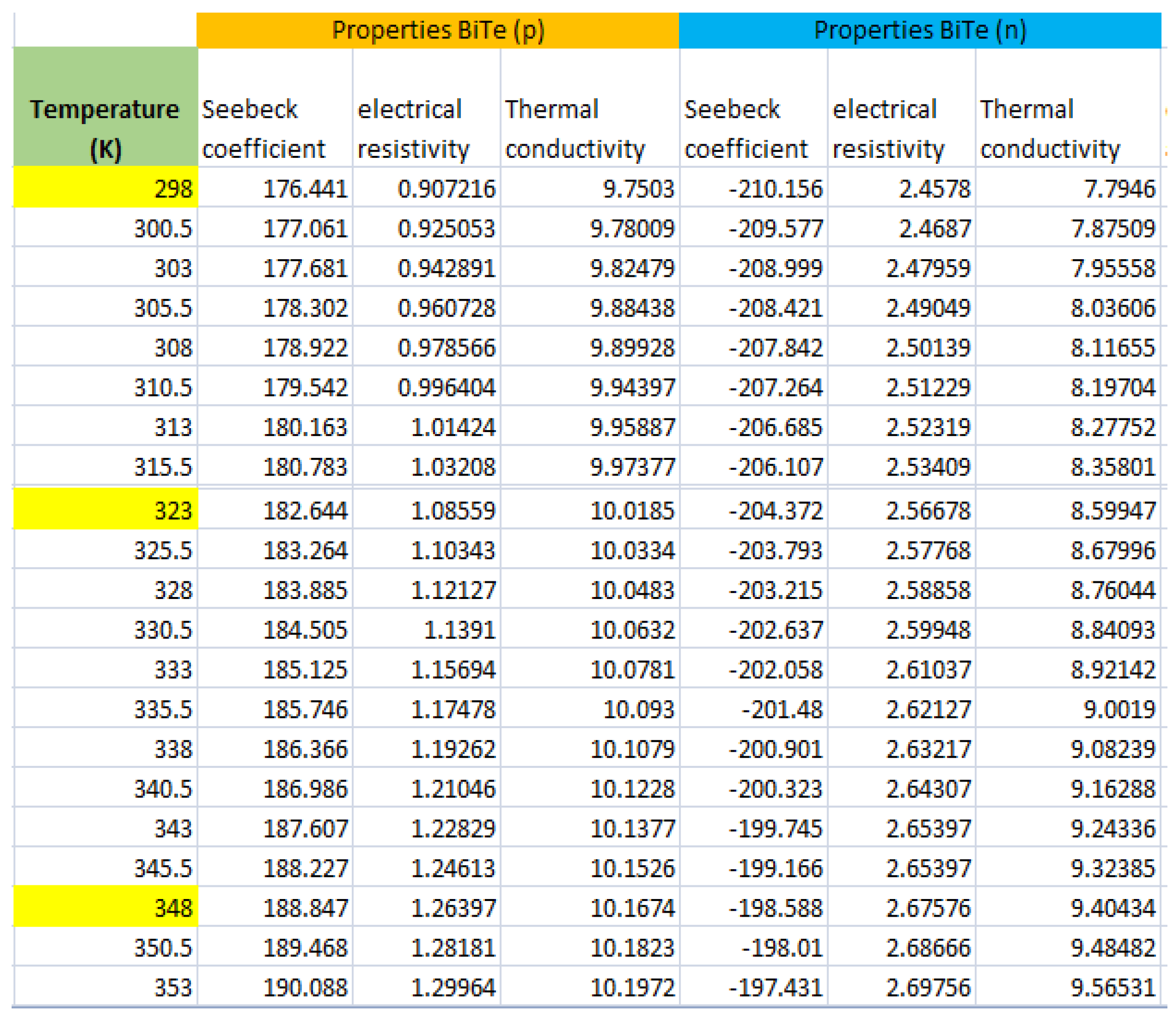
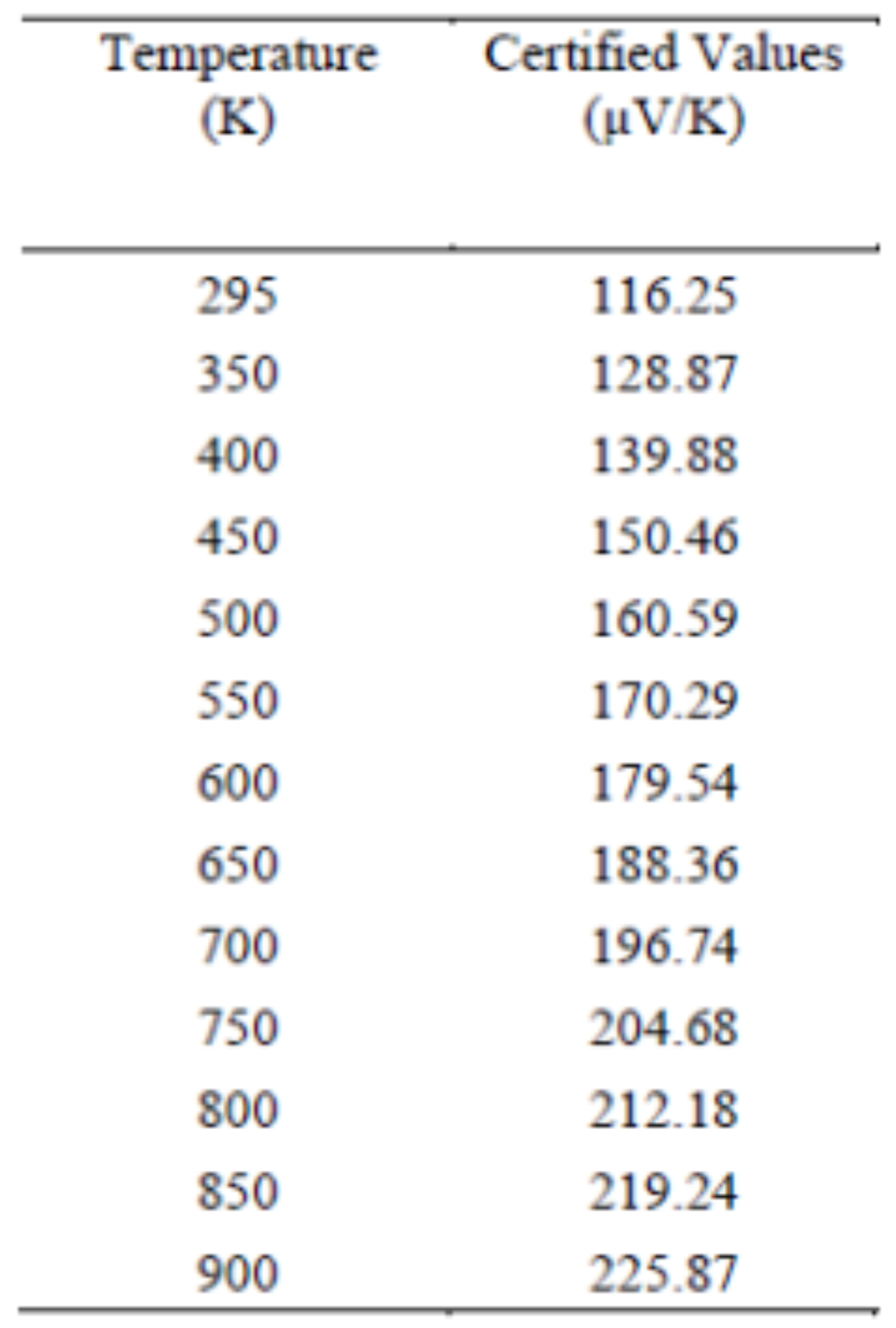
4. Temperature-Dependent Thermoelectric Properties and Supervised Machine Learning

Integrals [5,6] could be calculated thanks to the fact that we know the measurements of the thermoelectric properties at the temperatures in Table 2, generating a first $TEG$ design with their respective parameters $(A_n,A_P,l)$. However, the system obtained is specific for that temperature range, in such a way that it is not possible to adjust the design for a wider or narrower range. Trying to make a new design may require preparing a new material sample for new measurements or perhaps using advanced software for numerical design and simulation; there is a possibility that researchers do not have some of these resources. This difficulty can be overcome with the implementation of a supervised machine learning algorithm that allows predicting the values of the Seebeck coefficient, $\alpha$; electrical resistivity, $\rho$; and thermal conductivity, $\kappa$, properties at any temperature value.

Table 3. Experimental data of the thermoelectric properties of the $B{i}_{2}T{e}_3$ material.

T (K)	${\mathit{\alpha }}_{\mathit{p}}$ (µV/K)	${\mathit{\rho }}_{\mathit{p}}$ (${10}^{-3}\mathsf{\Omega }$cm)	${\mathit{\kappa }}_{\mathit{p}}$ (mW/cm K)
$T_0=298$	173	$0.927$	$9.63$
$T_1=323$	185	$1.015$	$9.85$
$T_2=348$	194	$1.198$	$9.87$
$T_3=373$	200	$1.415$	$9.79$
$T_4=398$	203	$1.632$	$9.70$
$T_5=423$	204	$1.834$	$9.71$
	${\mathit{\alpha }}_{\mathit{n}}\mathbf{\left(}\mathbf{\mu }\mathbf{V}/\mathbf{K}\mathbf{\right)}$	${\mathit{\rho }}_{\mathit{n}}\mathbf{\left(}{\mathbf{10}}^{-\mathbf{3}}\mathsf{\Omega }\mathbf{cm}\mathbf{\right)}$	${\mathit{\kappa }}_{\mathit{n}}\mathbf{(}\mathbf{mW}\mathbf{/}\mathbf{cm}\mathbf{K}\mathbf{)}$
	$-209$	$2.38$	8
	$-213$	$2.61$	$8.23$
	$-210$	$2.79$	$8.72$
	$-201$	$2.90$	$9.8$
	$-187$	$2.94$	$10.92$
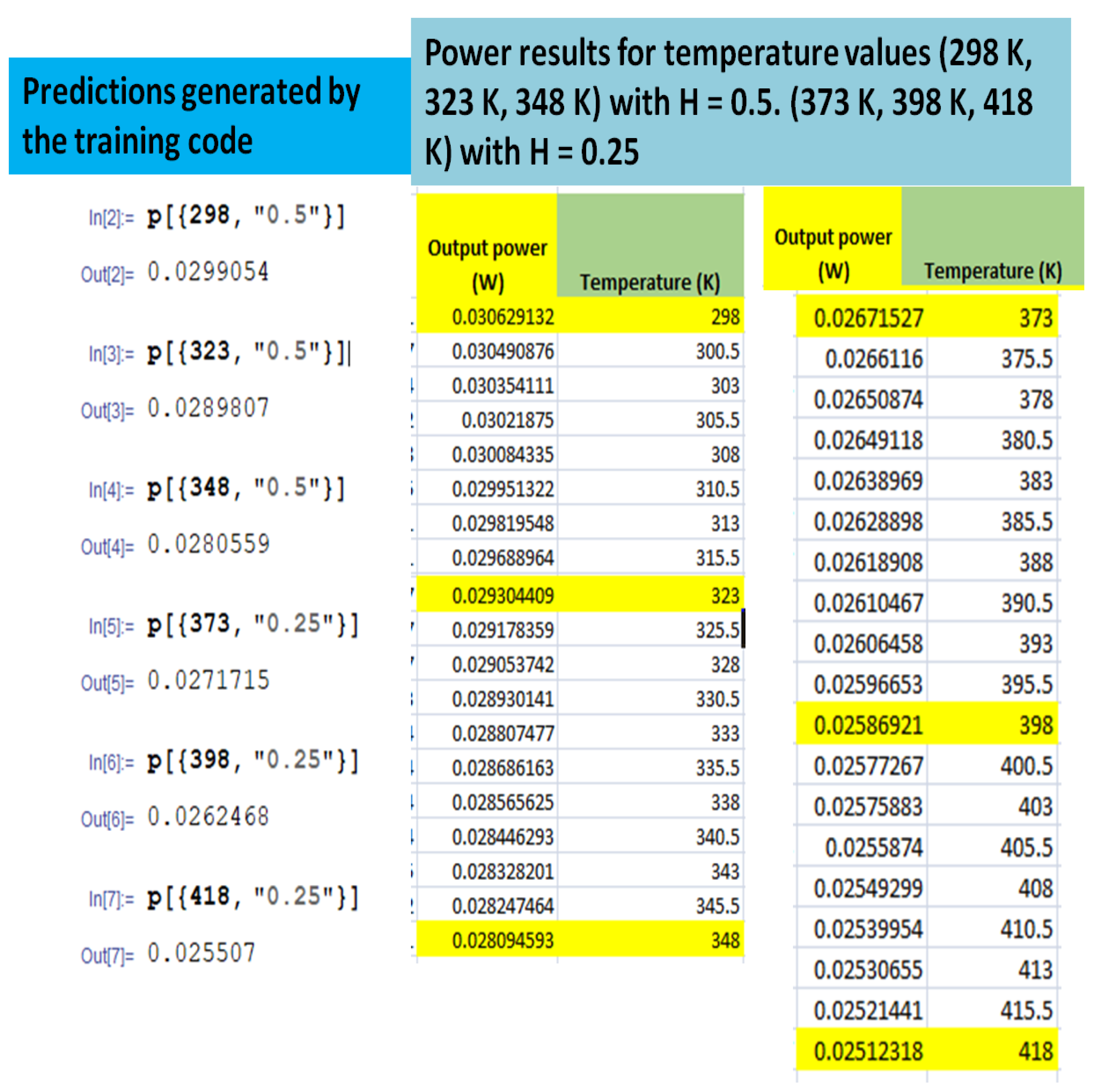
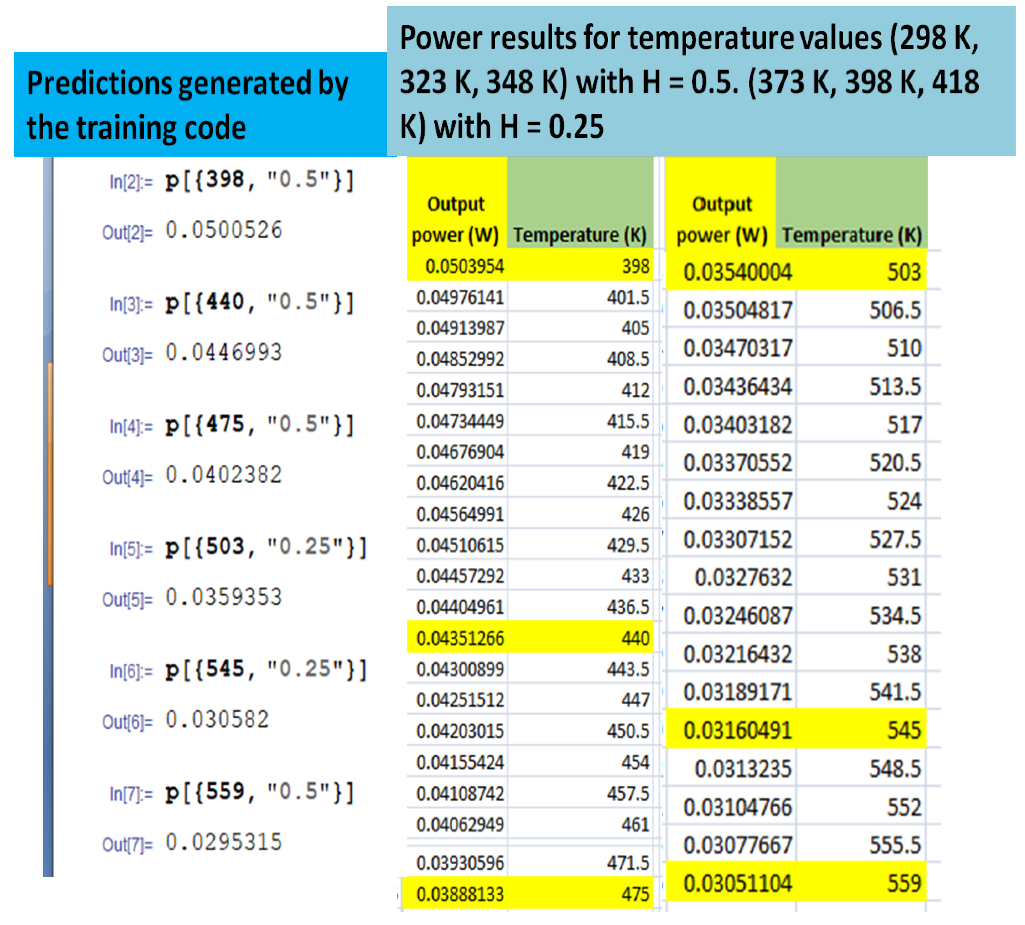
	$-171$	$2.92$	$12.07$

shows the measurements of these properties for the $BiTe$ material.

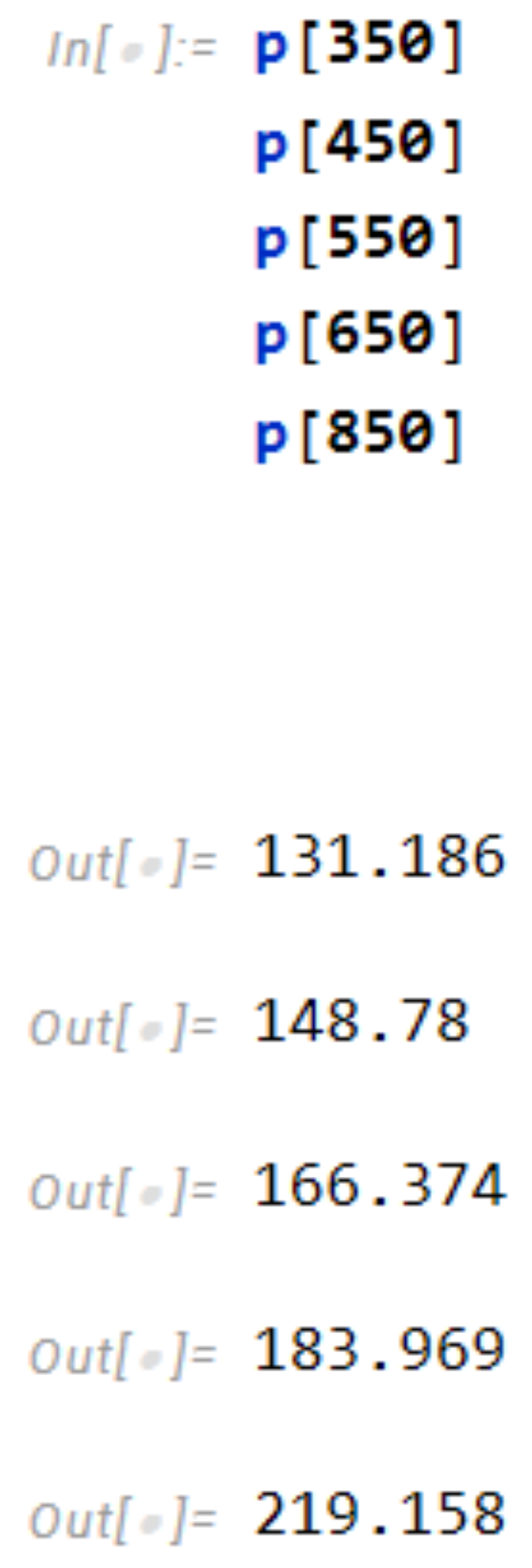
The data in Table 3 were used to train the prediction code, for which an 80/20 rule was used; that is, $80\%$ of the data were used for the training set and $20\%$ for the test set. The code was generated using the Wolfram Mathematica 13.2 software using a predictive function that has the advantage of automatically selecting the most appropriate prediction model according to the behavior of the experimental data used for training. Specifically, the algorithm was applied to obtain a set of 50 data points for each thermoelectric property; however, more data can be predicted for any established temperature range. The distance between the data was reduced to $2.5$ K. 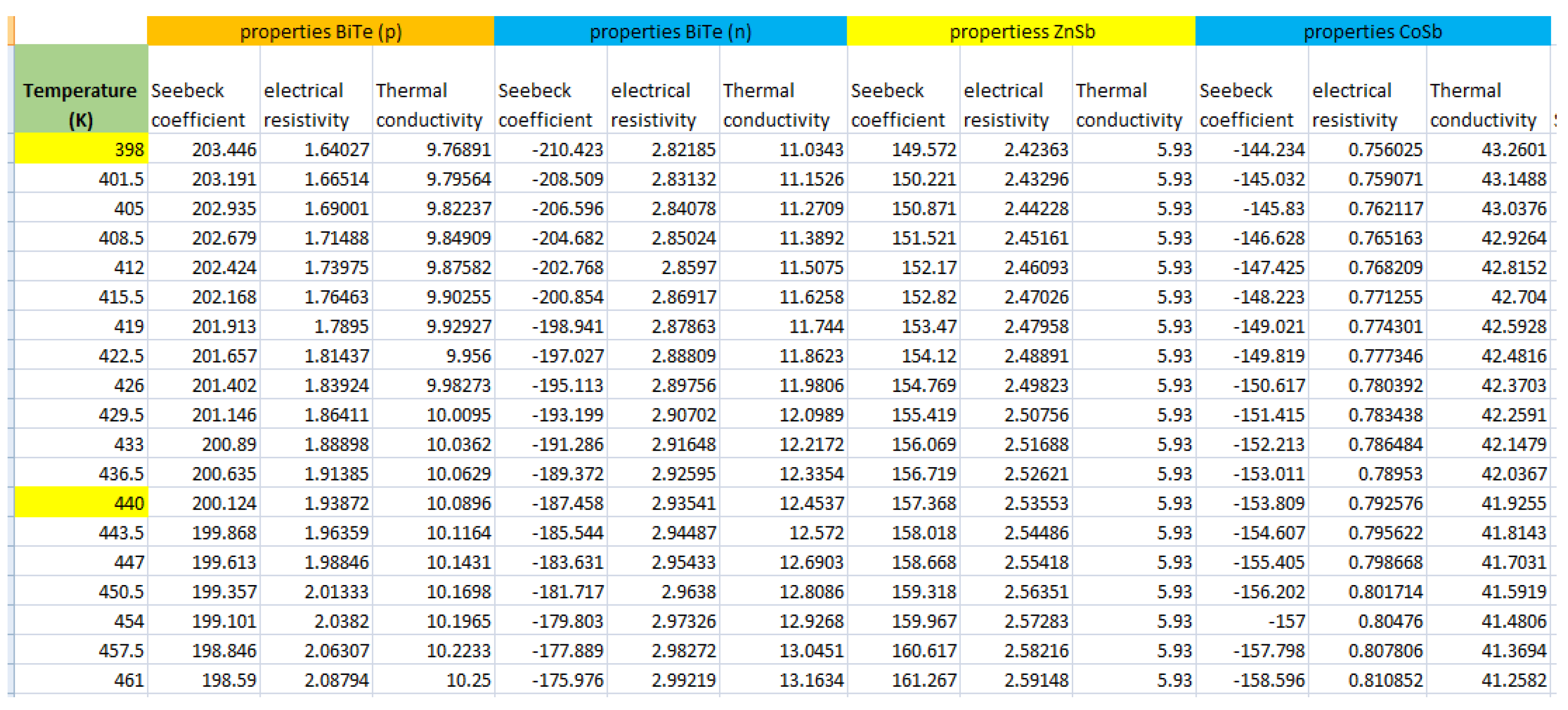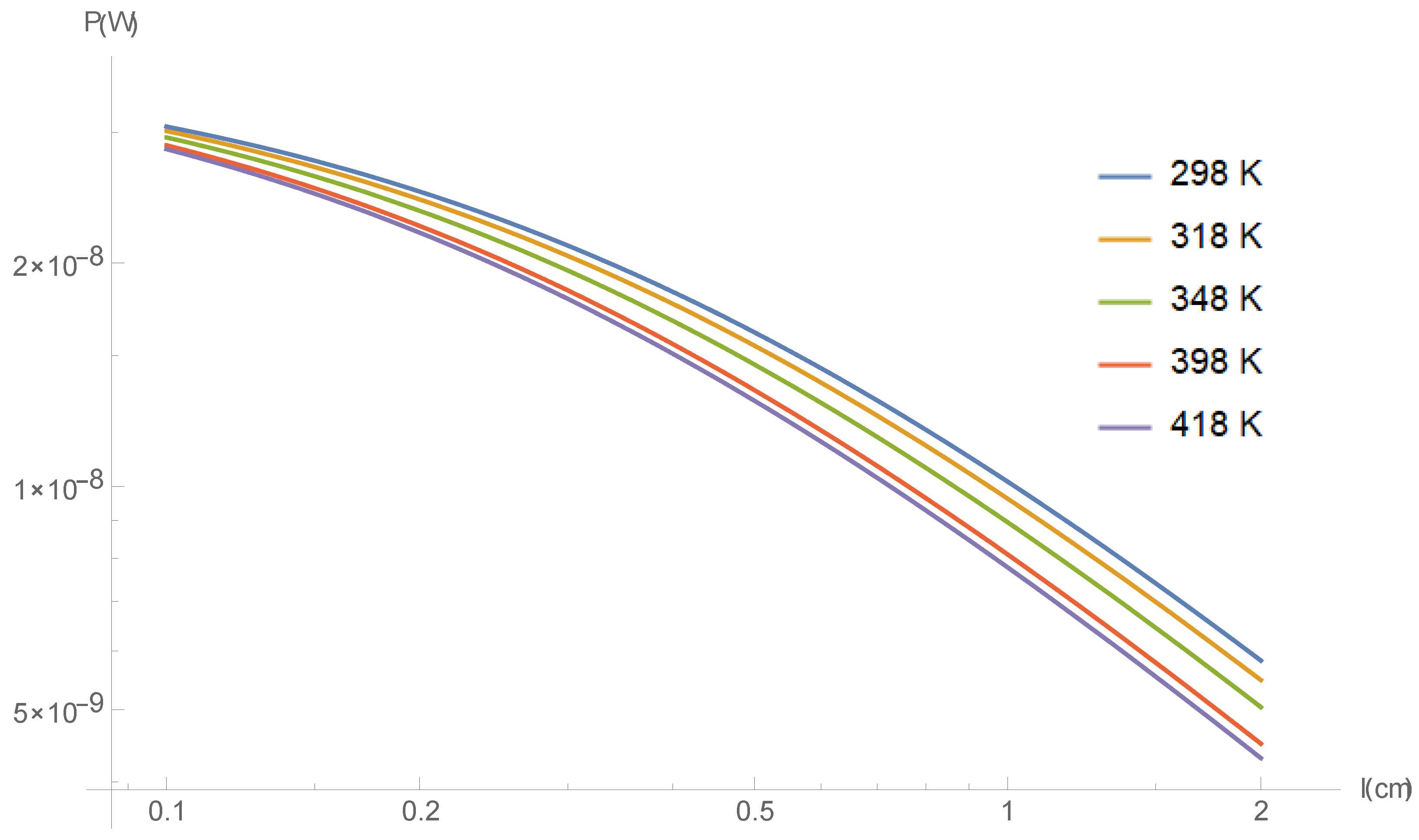Figure 2 shows a spreadsheet containing the prediction results of the thermoelectric properties generated by the algorithm for each of the materials selected for the design of the conventional generator.

This algorithm helps predict a material’s thermoelectric property value for any operating temperature value. As shown below, it is possible to calculate the maximum electrical power of a conventional system for any T value within this range.

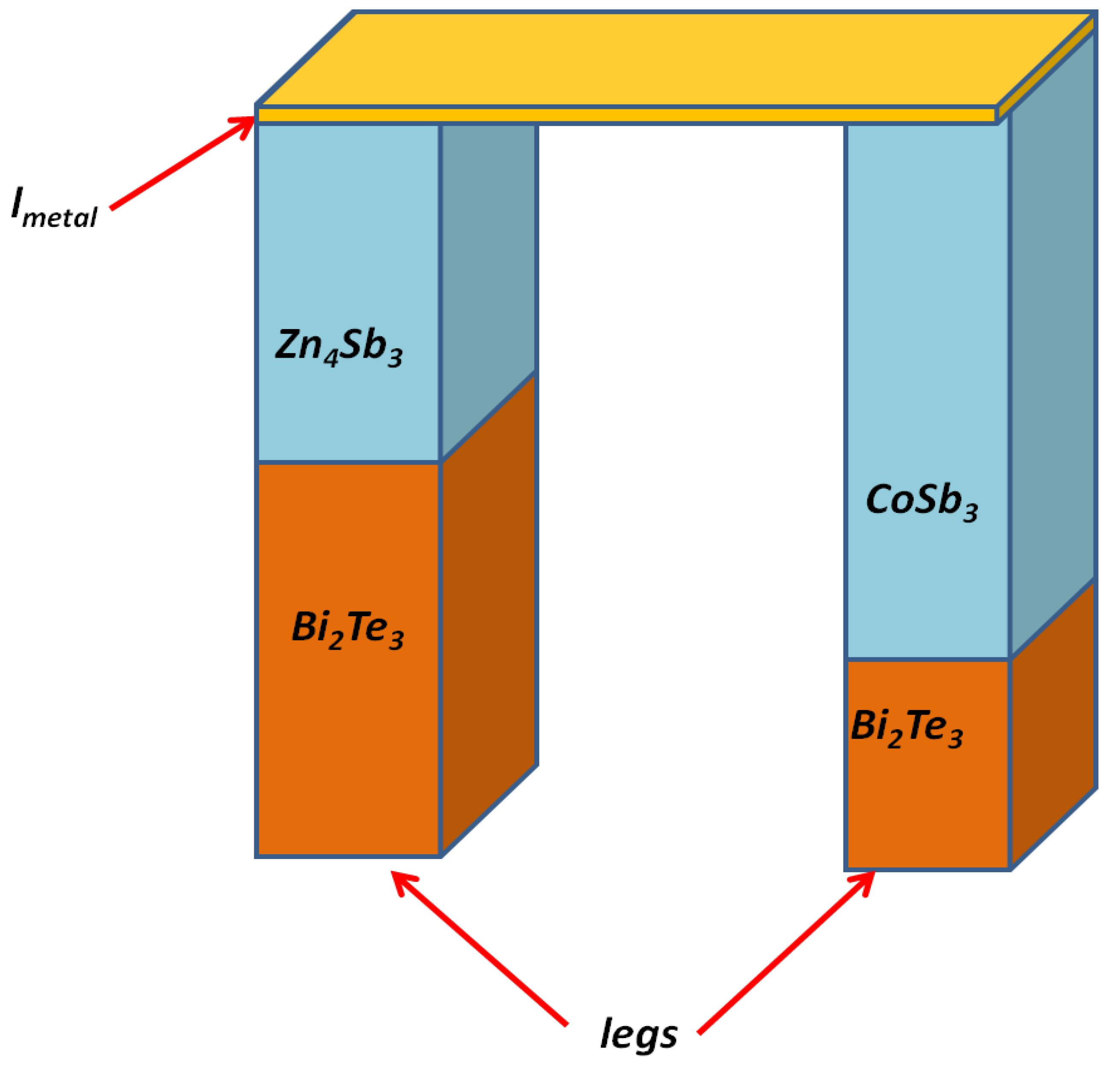
4.1. Segmented Thermocouple

As a result of efforts to take advantage of heat in a wide temperature range, the segmentation technique was developed. It consists of joining segments of various thermoelectric materials and allowing thermal and electrical contact between them; its principle is based on the fact that each of the segments will be subjected to the temperature range in which it reaches its highest figure of merit value.

4.1.1. Design of a Segmented Thermocouple

The materials selected were $B{i}_{2}T{e}_3$ and $Z{n}_{4}S{b}_3$ (p-type) and $B{i}_{2}T{e}_3$ and $CoS{b}_3$ (n-type). The operating temperatures selected were $T_C=398$ K and $T_H$ = 573 K.

Table 4. Numerical data of the $u\kappa$ product of the material $B{i}_{2}T{e}_3$.

T (K)	${\mathit{u}\mathit{\kappa }}_{{\mathrm{Bi}}_2{\mathrm{Te}}_3}$ (1/V)
398	$0.8466$
423	$0.8603$
448	$0.8932$
473	$0.3339$

and

Table 5. Numerical data of the $u\kappa$ product of the material $Z{n}_{4}S{b}_3$.

T (K)	${\mathit{u}\mathit{\kappa }}_{{\mathrm{Zn}}_4{\mathrm{Sb}}_3}$ (1/V)
482	$0.3167$
498	$0.4999$
523	$0.5107$
548	$0.5257$
573	$0.5430$

show the values of the product $uk$ of the materials $B{i}_{2}T{e}_3$ and $Z{n}_{4}S{b}_3$ (p-type), respectively.

Table 6. Numerical data of the $u\kappa$ product of the material $B{i}_{2}T{e}_3$.

T (K)	${\mathit{u}\mathit{\kappa }}_{{\mathit{Bi}}_{\mathbf{2}}{\mathit{Te}}_{\mathbf{3}}}$ (1/V)
398	$-0.6933$
423	$-0.4454$

and

Table 7. Numerical data of the $u\kappa$ product of the material $CoS{b}_3$.

T (K)	${\mathit{u}\mathit{\kappa }}_{{\mathbf{CoSb}}_{\mathbf{3}}}$ (1/V)
440	$-0.7948$
448	$-2.4649$
473	$-2.4387$
498	$-2.4164$
523	$-2.3984$
548	$-2.3855$
548	$-2.3783$
573	$-2.3783$

show the values of the product $uk$ of the materials $B{i}_{2}T{e}_3$ and $CoS{b}_3$ (n-type), respectively.

Applying the treatment defined in the previous sections, the following parameters of the segmented thermocouple were obtained:

Table 8. Current density and dimensional parameters of the segments.

Parameter	Bi${}_2$Te${}_3$ $\mathbf{\left(}\mathit{p}\mathbf{\right)}$	Zn${}_4$Sb${}_3$ $\mathbf{\left(}\mathit{p}\mathbf{\right)}$	Bi${}_2$Te${}_3$ $\mathbf{\left(}\mathit{n}\mathbf{\right)}$	CoSb${}_3$ $\mathbf{\left(}\mathit{n}\mathbf{\right)}$
$J(\mathrm{mA}/{\mathrm{cm}}^2)$	$29.16$	$29.16$	$96.96$	$96.96$
$l\left(\mathrm{mm}\right)$	$1.76$	$1.56$	$0.10$	$3.21$
$A\left({\mathrm{mm}}^2\right)$	$0.77$	$0.77$	$0.23$	$0.23$

contains the design parameters of the segmented thermoelectric generator. A design sketch is shown in Figure 3.

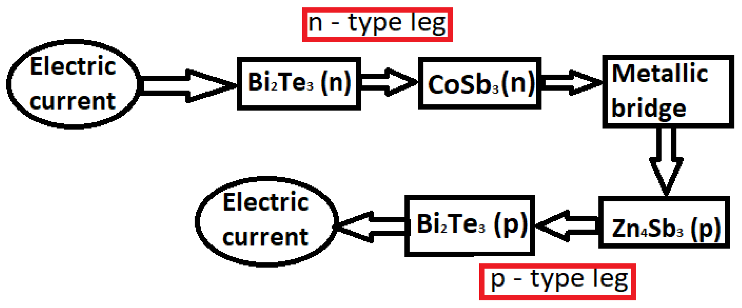
Figure 4 shows a diagram that represents the interaction between the components in the system.

Again, the prediction algorithm was applied to obtain 50 data points for each of the thermoelectric properties. For each of the materials selected in the design, the distance between the data points was reduced to $2.5$ K. Figure 5 shows a spreadsheet containing the prediction results of the thermoelectric properties generated by the algorithm for each of the materials selected for segmented generator design.

This algorithm helps predict the values of the materials’ thermoelectric properties for any operating temperature value within the range of 398–573 K. As shown below, it is possible to calculate the maximum electrical power of the segmented system for any T value within this range.

4.1.2. Evaluation of the Feasibility of the Segmented Thermocouple by Means of the Compatibility Factor

An important aspect to remember in the design of segmented thermocouples is that only certain combinations of materials are appropriate, because there is a risk of building a thermocouple with a low efficiency, even lower than that of a conventional thermocouple. A useful resource for evaluating combinations of materials is the compatibility factor $\left(S\right)$ [10], defined as

$$S=\frac{\sqrt{1+Z\overline{T}}-1}{\alpha \overline{T}}$$

(15)

Applying Equation (15), it can be confirmed that the materials selected in the system studied in this work were correct for the segmentation; see

Table 9. Values of the compatibility factor S for each of the materials selected for segmentation.

Material	S
$B{i}_{2}T{e}_3$$\left(p\right)$	$4.22$
$Z{n}_{4}S{b}_3$	$4.383$
$B{i}_{2}T{e}_3$$\left(n\right)$	$2.27$
$CoS{b}_3$	$2.26$

. In this table, it can be observed that the values of S between p-type and n-type materials differed by a factor not greater than 2, as indicated by the rule.

5. Results and Discussion

5.1. Maximum Electrical Power of a Conventional Thermocouple

As is well known in the field of thermoelectricity, the maximum power $\left(P_{max}\right)$ of the generator is reached with the condition $R_{load}=R_{internal}$. In this work, an analysis of the maximum power of generators, conventional and segmented, was conducted for various physical conditions established for the dimensional parameters (cross-sectional area, length of the legs, space between the legs). First, the maximum power analysis is shown for the conventional system and later for the segmented system.

The maximum power of a conventional $TEG$ is

$$\begin{array}{c}\hfill P_{max-conventional}=\frac{{({\alpha }_p-{\alpha }_n)}^2{(T_H-T_C)}^2}{4\left(R_n+R_p+R_{met}\right)}.\end{array}$$

(16)

$P_{max-conventional}$ was analyzed for three conditions, as a function of (a) the space between the legs $\left(H\right)$, (b) the ratio of cross-sectional areas $(A_p/A_n)$, and (c) the length of the legs $\left(l\right)$. Equation (16) was written for each of these parameters using relationships $R_n=\frac{{\rho }_{n}l}{A_n}$, $R_p=\frac{{\rho }_{p}l}{A_p}$, and $R_{metal}=\frac{{\rho }_{metal}l}{A_{metal}}$.

The electrical resistance $\left(R\right)$ metal used in this study is presented in

Table 10. Electrical resistance metal bridge.

Component	Electrical Resistance $\left(\mathit{R}\right)$
Metal	$\frac{0.00002\left(0.01\right)}{A_{metal}}$

. Notice that for calculation purposes, a thickness of the metal bridge of $0.01$ cm was selected.

We have chosen not to present the equations, since our main objective was to analyze the behavior of the power curves. The results obtained for each one are shown below.

5.1.1. Maximum Power of the Conventional Generator: Space between the Legs

The space between the thermoelectric legs is considered a variable parameter; see Figure 6.

Figure 7 shows the maximum electrical power as a function of the space between the legs for different values of temperature using the prediction algorithm. The values 298 K, 318 K, 348 K, 398 K, and 418 K were selected.

Figure 7 shows that the maximum power increased significantly in the range from 0 to 1 cm, after which the variation was insignificant. This is because the closer the legs are together, the greater the temperature difference between the hot and cold sides of the generator. It was also observed that the power values increased as the temperature decreased.

5.1.2. Maximum Power of the Conventional Generator: Area Ratio

It is also helpful to observe how the maximum power varies concerning the ratio of areas, to determine the optimum value of the $A_p$ and $A_n$ areas, which must be maintained for the system to achieve the highest possible power value.

Figure 8 shows the region of rapid increase in each electrical power curve. The electrical power quickly grew until reaching close to $0.5$; after that point, the variation was insignificant. Again, the maximum power was more significant for temperatures close to 298 K.

5.1.3. Maximum Power of the Conventional Generator: Length of the Legs

From the variation in the maximum power as a function of the length of the legs, it was possible to determine the optimum length for the highest performance of the thermoelectric generator.

Figure 9 shows that for the selected temperatures, length values less than 0.1 cm would be appropriate to achieve the maximum performance.

5.2. Maximum Electrical Power of a Segmented Thermocouple

The maximum power produced by a segmented thermoelectric generator is defined using the following equation:

$$\begin{array}{c}\hfill P_{max-segmented}=\frac{{({\alpha }_{p-effective}-{\alpha }_{n-effective})}^2{(T_H-T_C)}^2}{4\left(R_{n1}+R_{n2}+R_{p1}+R_{p2}+R_{met}\right)}\end{array}$$

(17)

Note that the effective Seebeck coefficient can be defined for each of the n-type and p-type segmented legs as

$${\alpha }_{p-effective}=\frac{{\kappa }_{p1}{\alpha }_{p2}+{\kappa }_{p2}{\alpha }_{p1}}{{\kappa }_{p1}+{\kappa }_{p2}}$$

(18)

$${\alpha }_{n-effective}=\frac{{\kappa }_{n1}{\alpha }_{n2}+{\kappa }_{n2}{\alpha }_{n1}}{{\kappa }_{n1}+{\kappa }_{p2}}$$

(19)

The electrical power produced by the segmented thermoelectric generator was analyzed for four conditions, which were (a) as a function of the space between the legs, $\left(H\right)$, (b) as a function of the ratio of cross-sectional areas, $(A_p/A_n)$, (c) as a function of the ratio of the lengths of p-type materials $(l_{p2}/l_{p1})$, and (d) as a function of the ratio of lengths of n-type materials $(l_{n2}/l_{n1})$. Similarly to the case of the conventional thermocouple, Equation (17) was written for each of the four parameters. Again, the key was the electrical resistance values, which in this case were $\left(R_{n1}\right)$, $\left(R_{n2}\right)$, $\left(R_{p1}\right)$, $\left(R_{p2}\right)$, and $\left(R_{met}\right)$. Thus, the power curves for each were generated.

5.2.1. Maximum Power of the Segmented Thermoelectric Generator: Space between the Legs

Figure 10 shows that the system’s maximum power was practically constant as the space between the legs changed, but this depended dramatically on the selected temperatures. It can also be seen that the temperature that produced the highest power was 510 K. This is interesting news for researchers and engineers who are working on developing new ways to generate power. The results of this study suggest that by carefully controlling the temperature, we could produce a constant and reliable source of power, regardless of the distance between the legs of the system. This could have a major impact on the development of new technologies, such as portable electronics and renewable energy sources.

5.2.2. Maximum Power of the Segmented Thermoelectric Generator: Area Ratio ($A_p/A_n$)

Figure 11 shows the maximum power for the segmented thermoelectric generator as a function of the area ratio. An attractive characteristic is the different intersections of the curves in the interval from 0 to $0.5$. These intersection points are essential because they represent the same maximum power at different temperatures and at the same area ratio. This behavior results from the segmentation because, as it is well known, certain thermoelectric materials are more efficient than others at different temperatures. As the values of the area ratio after that interval increased, all the curves remained without notable changes. This analysis shows that the maximum power output of a segmented TEG can be increased by increasing the area ratio and operating the $TEG$ at a temperature of 510 K.

5.2.3. Maximum Power of the Segmented Thermoelectric Generator: n-Type Length Ratio

In the case of the conventional thermocouple, analyzing the power variation as a function of the leg lengths is a simple task because $lp=ln$. However, for the case of a segmented $TEG$, the lengths are different for each segment; that is, a set of four lengths is formed ($l_{n1}$, $l_{n2}$, $l_{p1}$, and $l_{p2}$). A practical method is to analyze the electrical power as a function of the length ratios ($l_{n2}/l_{n1}$) and ($l_{p2}/l_{p1}$). Figure 12 shows the power of the segmented system as a function of the ratio $(l_{n2}/l_{n1})$ at different temperatures. The power was maximum for small values of ($l_{n2}/l_{n1}$) or when ($l_{n2}<l_{n1}$), but it decreased when this ratio increased; that is, ($l_{n2}>l_{n1}$). The temperature that showed the highest power value was $T=426$ K. This result suggests that the segmented system was more efficient at generating power at small values of n-type length ratio. Notice that the electrical power decreased rapidly from the value $0.5$.

5.2.4. Maximum Power of the Segmented Thermoelectric Generator: p-Type Length Ratio

Figure 13 shows the maximum power as a function of the ratio $(l_{p2}/l_{p1})$ for different temperatures. An important feature is that the electrical power decreased rapidly for all intervals of values of the p-type leg ratio ($l_{p2}/l_{p1}$). This is because longer legs have more resistance, which limits the current flow and therefore the power output. Notice that the maximum power values of the system in this case were lower than those achieved with the quotient $(l_{n2}/l_{n1})$. These results suggest that for maximum electrical power, semiconductors should be segmented in n-type legs. This can reduce the resistance of the legs and allow for more current to flow, resulting in a higher power output. The highest maximum power output was achieved at temperatures around 398 K. The electrons in the semiconductor were more mobile at higher temperatures.

When comparing the two systems, conventional and segmented, regarding the space parameter $\left(H\right)$ between the legs, the changes in maximum power values are more noticeable in the curves of the conventional thermocouple. In contrast, for the segmented thermocouple, the variations are minimal. The maximum power stabilized after reaching a maximum value at some specific value of H, because this parameter is related to the area of the metal bridge; thus, when H increased, the resistance of the metal bridge decreased and approaches zero. In this way, the maximum power value approached a constant value. In the case of the segmented thermocouple, it can be seen from Figure 10 that a smaller value of H$(0\le H\le 1)$ was required to reach the maximum power and stability, compared to the value of H required for the conventional thermocouple $(1\le H\le 2)$; see Figure 6. When analyzing the variation in power as a function of $(A_p/A_n)$, both systems reached maximums at similar points $(A_p/A_n\approx 0.5)$, after which it was no longer necessary to continue increasing the ratio. It is very interesting to observe the intersections between the power curves in Figure 11; it is possible that this was a consequence of the segmentation technique used (remember that each segment of thermoelectric material reached its maximum performance value for a specific temperature). Moreover, the intersection point of two or more of these curves indicates that at those temperatures the $TEG$ was operating with the segments at maximum efficiency. For example, in the interval $0<A_p/A_n\le 0.5$, the power curve at 559 K intersects with the curves at 398 K, 426 K, and 450.5 K. When comparing the points of intersection with the temperature values of Table 4, Table 5, Table 6 and Table 7, the following correspondence is found: “for a ratio of (Ap/An = 0.5), the optimal temperature values of each material are shown in

Table 11. Optimum temperature values for each segment.

T (K)	Material
559	$Z{n}_{4}S{b}_3$ (p)
$450.5$	CoSb${}_3$ (n)
426	$B{i}_{2}T{e}_3$ (p)
398	$B{i}_{2}T{e}_3$ (n)

”.

For the analysis of the maximum power as a function of the leg length (conventional $TEG$) or the ratio of lengths (segmented $TEG$), the Figure 9, Figure 12 and Figure 13 suggest that small values of these parameters favor the performance of the systems, because it is possible to reduce the electrical resistance.

The analysis of the temperatures in each case mentioned above showed that for the conventional thermocouple, the dominant temperature was 298 K. This result confirmed that the BiTe material reached its maximum figure of merit value at an operating temperature between 200 and 300 K. On the other hand, regarding the segmented thermoelectric generator, Figure 10 and Figure 11 show that the temperature that produced the highest power was 510 K. However, in Figure 12, the segmented system produced the highest maximum power value at 426 K, while Figure 13 shows that at T = 398 K, the system generated a high maximum power value. These peculiarities show that, unlike the conventional thermocouple, in the case of the segmented thermocouple, there was a greater sensitivity to changes in the operating temperature, in a specific way concerning the condition established for certain dimensional parameters.

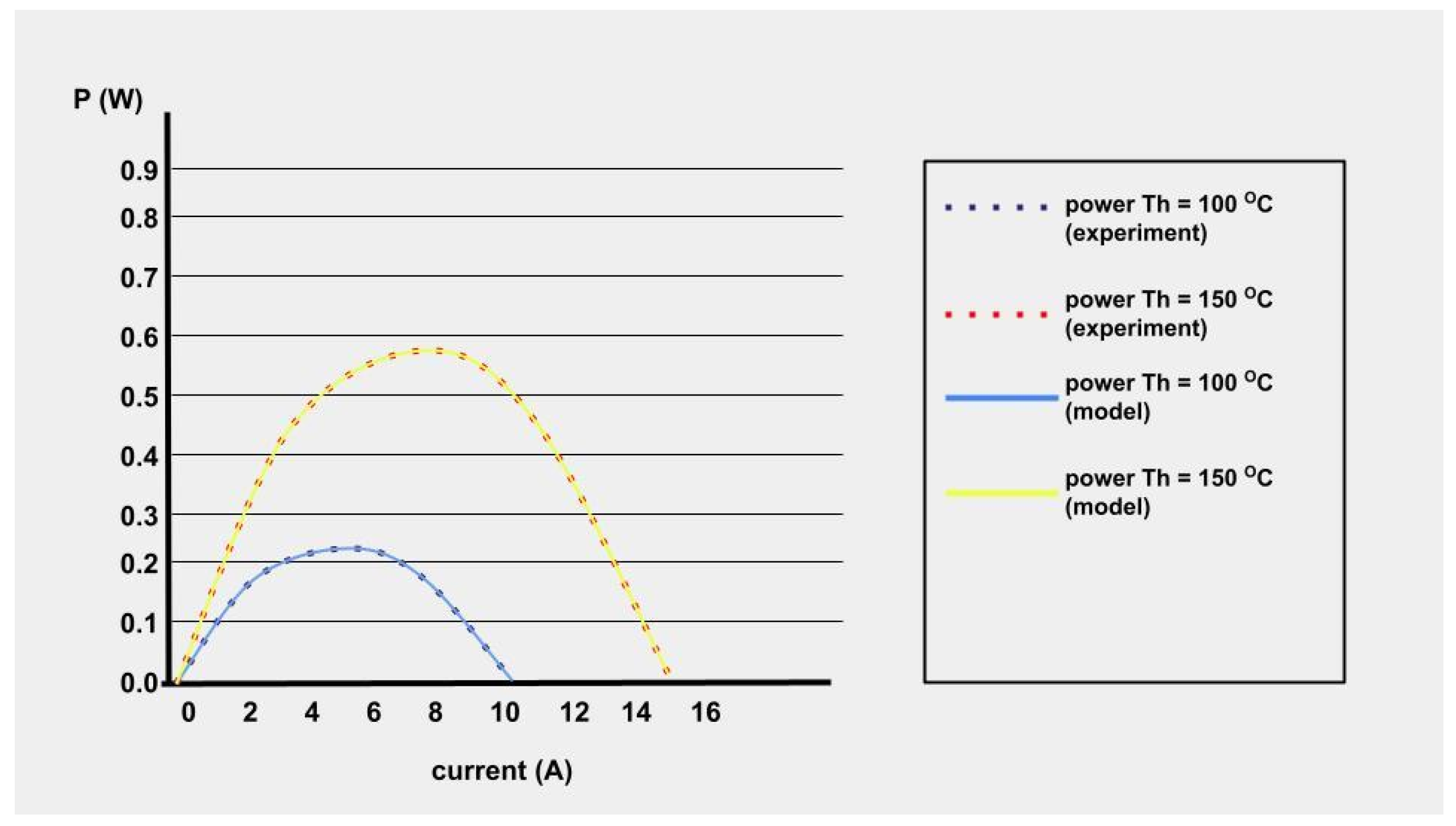
6. Model Building and Experimental Setup

In order to verify the validity of the proposed methodology, in this section, we consider the results of the work of Crane et al. [17], who created a design using a computerized model and performed an experiment with the built prototype of a system called a three-couple $TEG$ engine; see Figure 14 [17].

The test carried out for this work consisted of using the information from the experimental measurements to design a conventional $TEG$; however, unknown data were necessary to correctly develop the design. The source of the known information was the data provided by Crane’s paper [17], shown in

Table 12. $TEG$ engine data [17].

Material	Bi${}_2$Te${}_3$
$T_c$	$20{}^{°}\mathrm{C}=293.15$ K
$T_h$	$150{}^{°}\mathrm{C}=423.15$ K

.

Figure 15 shows the power curves against the electric current for certain values of $T_h$, obtained through the computerized model made by authors in [17]. It is observed that they coincide with the experimental curves.

Next, we sought to design a three-couple $TEG$ engine system applying the reduced variables methodology with supervised machine learning, to obtain a graph like the one shown in Figure 15. In addition to the data shown in Table 12, it was required to know the properties and dimensions $A_p$, $A_n$, $l_p$, $l_n$, ${\rho }_p$, ${\rho }_n$, $A_{metal}$, $l_{metal}$, and ${\rho }_{metal}$ not provided by [17], so it was necessary to calculate them.For this purpose, a first attempt was made, in which the Seebeck coefficient and electrical resistivity data from Table 3 were used to obtain the graph of power at temperature $T_h$ = 150 °C = 423.15 K, presented as the yellow curve in Figure 15. In this case, the six temperature values that are provided in Table 3 were the real values taken from the measurement and, as can be seen, the extreme values $T_c$ = 298 K = 24.85 °C and $T_h$ = 423 K = 149.85 °C were only approximate to the values actually required for the design ($T_c$ = 293.15 K = 20 °C and $T_h$ = 423.15 K = 150 °C). With this information, the reduced variables technique was applied to obtain a first design for the three-couple TEG engine, for which the graph of electrical power as a function of electrical current is shown in Figure 16.

A comparison between Figure 16 and the yellow curve in Figure 15 shows that the design obtained in this first attempt deviated from Crane’s model by approximately $50\%$, which is a very high margin. It was therefore necessary to adjust the six temperature values from Table 3 to the correct range of $T_c$ = 298 K = 24.85 °C and $T_h$ = 423 K = 149.85 °C. The following table shows the adjustment.

The values $u{\kappa }_n$, $u{\kappa }_p$, ${\alpha }_n$, ${\alpha }_p$, ${\rho }_n$, and ${\rho }_p$ (Table 2 and Table 3) were used as training data for the supervised machine learning code implemented in this work and thus generated appropriate data from these properties for the temperature values from

Table 13. Adjusted temperatures for the design of the $TEG$ engine.

T (K)
$T_0=293.15=20{}^{°}\mathrm{C}$
$T_1=319.15$
$T_2=345.15$
$T_3=371.15$
$T_4=397.15$
$T_5=423.15=150{}^{°}\mathrm{C}$

. The results are shown in the following

Table 14. Values $B{i}_{2}T{e}_3$ thermoelectric properties obtained by supervised machine learning model.

T (K)	${\mathit{u}}_{\mathit{p}}{\mathit{\kappa }}_{\mathit{p}}\mathit{dT}$ (A/cm)	${\mathit{\alpha }}_{\mathit{p}}$ (µV/K)	${\mathit{\rho }}_{\mathit{p}}$ (${10}^{-3}\mathbf{\Omega }$cm)
$T_0=293.15=20{}^{°}\mathrm{C}$	$0.8278$	193	$1.3975$
$T_1=319.15$	$0.8278$	193	$1.3976$
$T_2=345.15$	$0.8278$	193	$1.3976$
$T_3=371.15$	$0.85345$	194	$1.3977$
$T_4=397.15$	$0.85345$	194	$1.3978$
$T_5=423.15=150{}^{°}\mathrm{C}$	$0.85345$	$193.5$	$1.3979$
T (K)	${\mathit{u}}_{\mathit{p}}{\mathit{\kappa }}_{\mathit{p}}\mathit{dT}$ (A/cm)	${\mathit{\alpha }}_{\mathit{n}}$ (μV/K)	${\mathit{\rho }}_{\mathit{n}}$ (10−3 Ωcm)
$T_0=293.15=20{}^{°}\mathrm{C}$	$-0.5507$	$-209$	$2.7573$
$T_1=319.15$	$-0.5507$	$-209$	$2.7574$
$T_2=345.15$	$-0.5508$	$-210$	$2.7574$
$T_3=371.15$	$-0.5508$	$-210$	$2.7575$
$T_4=397.15$	$-0.5508$	$-187$	$2.7575$
$T_5=423.15=150{}^{°}\mathrm{C}$	$-0.5509$	$-171$	$2.7576$

.

Using the data from column two and applying the methodology with the set of Equations (2)–(12), the geometric parameters of the couples of the TEG engine were obtained, see

Table 15. Geometric parameters obtained for the design of the TEG engine of $B{i}_{2}T{e}_3$.

Parameter	Numerical Value
$l_n=l_p$	$1.85$ mm
$A_p$	$1.73$ mm${}^2$
$A_n$	$2.67$ mm${}^2$

.

Subsequently, with the data from the third and fourth columns, the averages of the quantities ${\alpha }_n$, ${\alpha }_p$, ${\rho }_n$, and ${\rho }_p$ in the temperature range ($T_c$ = 293.15 K = 20 °C and $T_h$ = 423.15 K = 150 °C) were obtained. The results are shown in

Table 16. Averaged Seebeck coefficient and electrical resistivity, $TEG$ engine design.

Property	Averaged Value
$\overline{{\alpha }_n}$	193.499 $\left(\mathsf{\mu }\mathrm{V}/\mathrm{K}\right)$
$\overline{{\alpha }_p}$	−201.111 $\left(\mathsf{\mu }\mathrm{V}/\mathrm{K}\right)$
$\overline{{\rho }_n}$	2.75749 ${\rho }_p\left({10}^{-3}\mathsf{\Omega }\mathrm{cm}\right)$
$\overline{{\rho }_p}$	1.39773 ${\rho }_p\left({10}^{-3}\mathsf{\Omega }\mathrm{cm}\right)$

.

The data obtained for the legs of the $TEG$ engine (Table 15 and Table 16), as well as the data of the metallic bridge (Table 10), were used in combination with the following equation for the power produced by the $TEG$ engine.

$$P_{TEG-engine}=n\left[({\alpha }_p-{\alpha }_n)(T_h-T_c)I-\left(\frac{{\rho }_n{l}_n}{A_n}+\frac{{\rho }_p{l}_p}{A_p}+\frac{{\rho }_{metal}{l}_{metal}}{A_{metal}}\right)I^2\right]$$

(20)

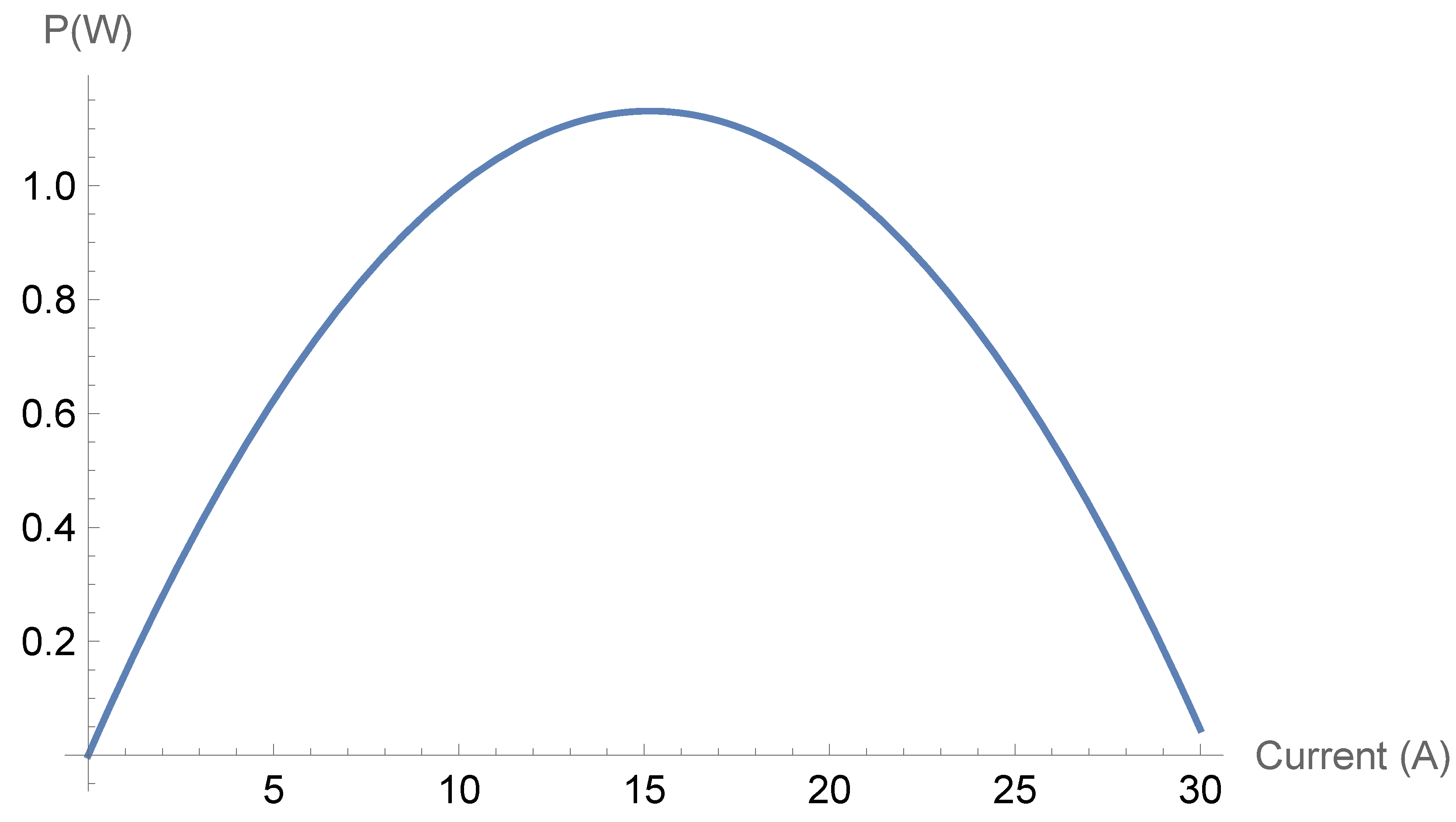
where $P_{TEG-engine}$ is the power produced by the TEG engine; n is the number thermocouples, which in this case is $n=3$; and I is the electric current (which is the independent variable and is measured in amperes). The other quantities that appear in Equation (20) have already been indicated above. The graph of the electrical power produced by the three-couple $TEG$ engine is shown in Figure 17.

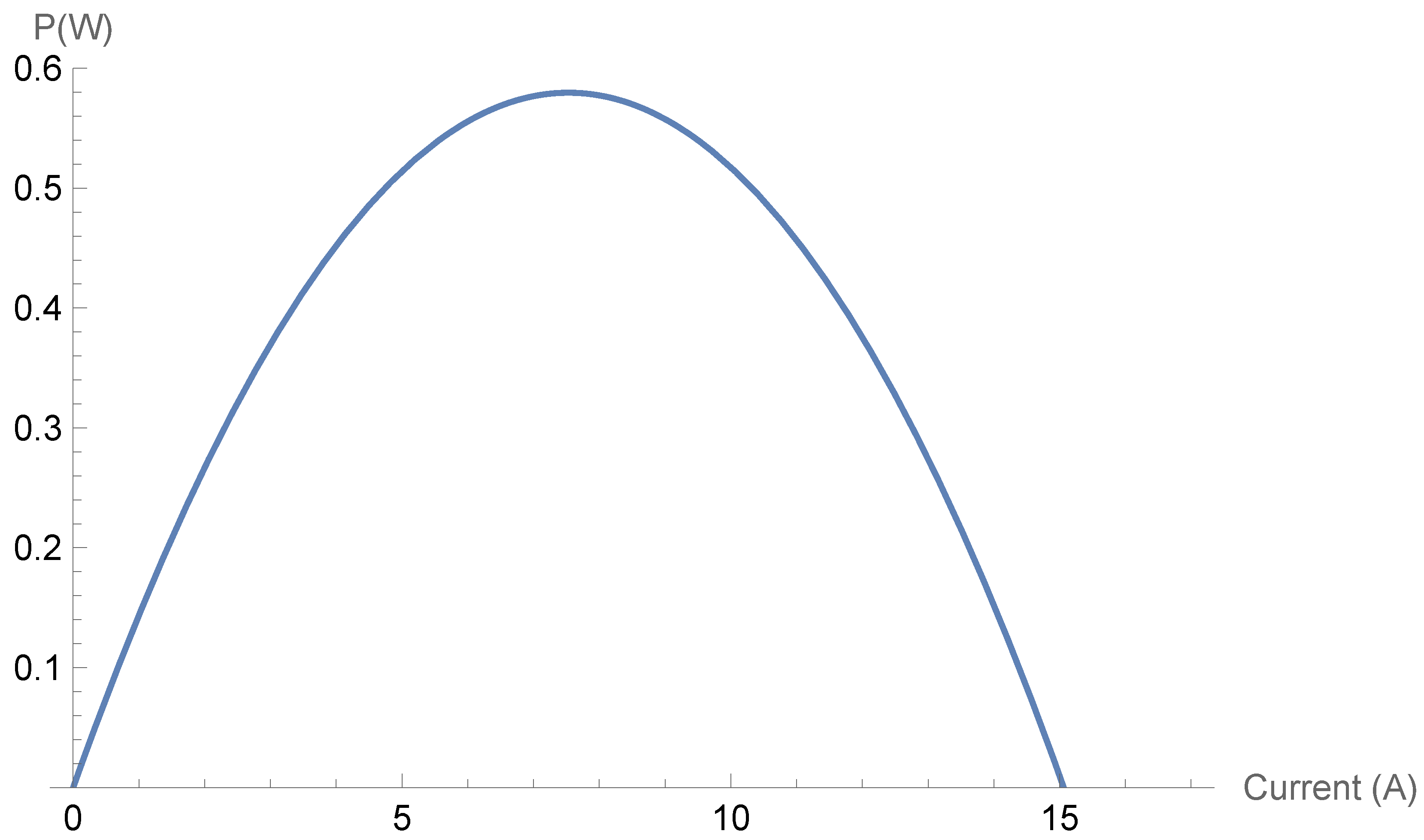
In Figure 17, it can be seen that the graph obtained adjusted well to the original Crane curve at $T_h$ = 150 °C (curve in yellow); see Figure 14. It can be seen that the same maximum value was reached below $0.6$ W around 8 A in a range of 0–15 A. Therefore, it is evident that the methodology (which combined the reduced variables method with supervised machine learning) proposed in this work managed to reproduce the three-couple $TEG$ engine model and the experiment of Crane et al. [17].

7. Conclusions

This work has shown that the fusion of supervised machine learning with the reduced variables technique can be a useful tool for designing $TEGs$ and adjusting them to the conditions imposed by the operating environment of the system, specifically when facing the challenge of knowing a reduced set of measured values. Thanks to its ability to calculate geometric and prediction parameters, it is possible to

(a) Approximate values of thermoelectric properties $(\alpha ,\rho ,\kappa )$ for any temperature value;

(b) Generate new data from few experimental values, even when it is not possible to perform a new experiment;

(c) Design $TEGs$ for any range of temperature; if the value of a thermoelectric property for a specific temperature is not known experimentally, it is possible to predict it with $\left(MLS\right)$ (Figure 2 and Figure 5) and use it for design calculations;

(d) Analyze power simultaneously with respect to various parameters for any temperature value and determine optimization conditions.

The previous characteristics were verified through the design and analysis of the power of the conventional $TEG$ (Section 3.1), segmented $TEG$ (Section 4.1), and $TEG$ engine (Section 6) systems.

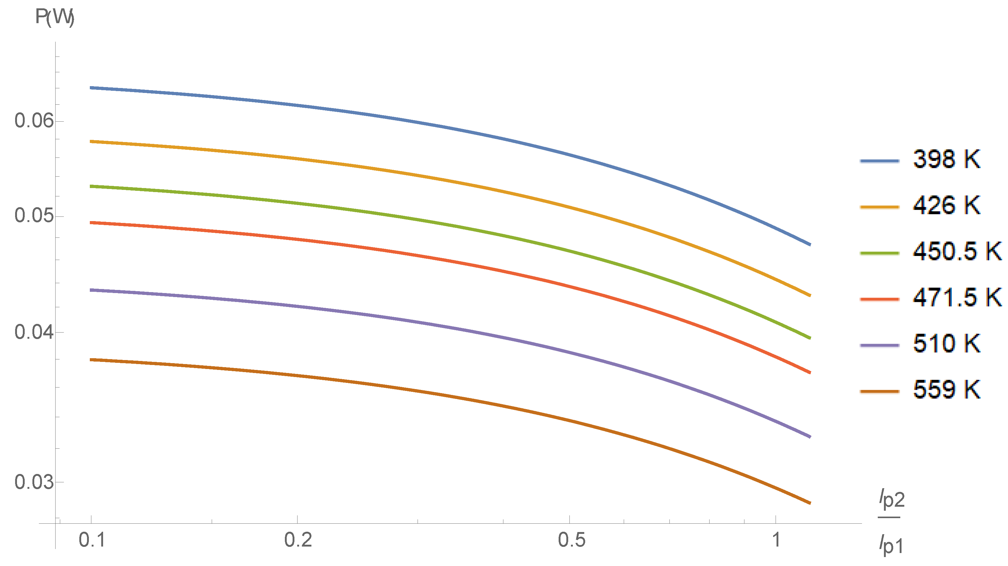
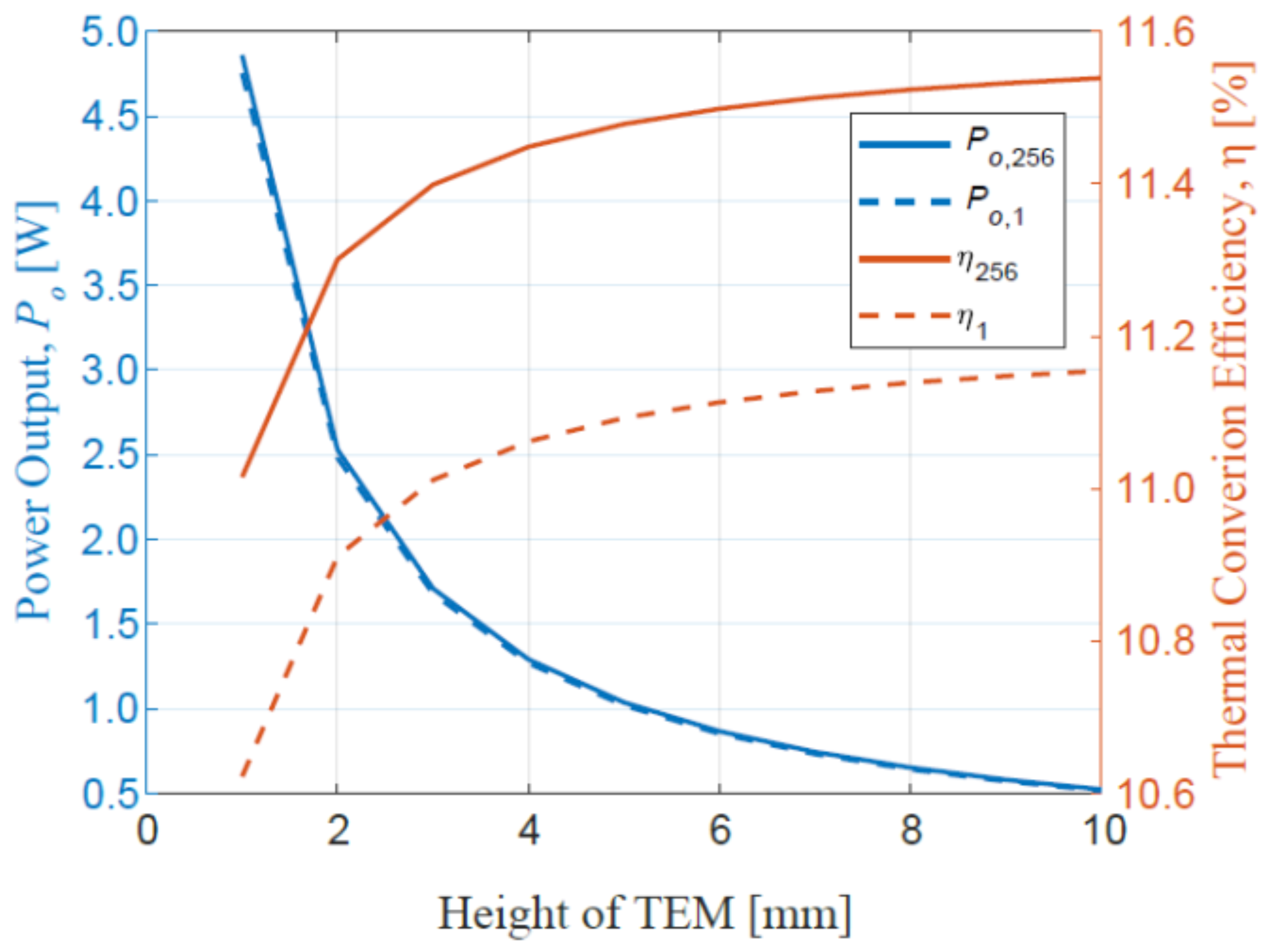
When conducting the power analysis, one of the outstanding findings was the result shown in Figure 11, indicating that the curve that corresponded to the highest temperature intersected with the curves of the other temperatures. Each intersection point specifically corresponds to the maximum performance of a segment. These intersection points occur very close to the value $(A_p/A_n)$ in which the power of the segmented $TEG$ is maximized.

As shown throughout this work, the proposed methodology was translated into a code in mathematics; its usability is now evaluated in terms of the following ten techno-economic aspects:

(1) The calculation scheme will be updated soon, to introduce a procedure based on heat transfer and to consider the physical aspects of the heat source;

(2) From an economic point of view, although Wolfram is a licensed software, it currently allows the user a free basic plan account, in which the code notebook could be published and shared with those interested in designing thermoelectric systems with this methodology;

(3) The code automatically selects the appropriate prediction method according to the training data. For the study of conventional and segmented systems, the methods that the code selected to predict the values were linear regression, decision tree, and first neighbors;

(4) The methodology could be transferred in code to another type of software that is freely available; for example, it could be implemented in python. In that case, there would be the advantage of being able to modify the prediction method and make more robust codes that can be better adjusted to the training data;

(5) This methodology may allow for the design of $TEGs$, taking advantage of the results of experimental measurements reported in various papers. This aspect is very useful for researchers who want to design $TEGs$ and who do not have a laboratory, the equipment to develop experiments, or specialized software for design and simulation;

(6) So far, the code has been tested with the thermoelectric materials $B{i}_{2}T{e}_3$, $Z{n}_{4}S{b}_3$, and $CoS{b}_3$. Currently, there are new materials, for example, organic materials or new alloys; thus, tests must be carried out using the properties of these new materials, to adapt the code to the needs of new $TEG$ applications.

(7) In addition to what is mentioned in point $\left(5\right)$, the designed code does not require high-end computing equipment compared to specialized design software. In the case of the calculations developed in this work, an AMD Ryzen 3 processor with Radeon Vega Mobile Gfx 2.60 GHz, with 8 GB RAM, was used;

(8) The methodology has only been applied for constant cross-sectional areas with a quadrangular geometry. The code should be extended to include the design of $TEGs$ with cross-sectional areas with geometries other than quadrangular, for example, circular. Variable cross-sectional areas regarding leg length could also be included. This could be achieved by reformulating Equations (16) and (17) in terms of $A_n$ and $A_p$;

(9) The code does not send any warning in the event that the user makes some type of error when capturing the information for the design; this still depends on the skills and knowledge of the user regarding the specifications of the system to be designed, but it is intended that soon some kind of table with reference values will be added to act as a design guide;

(10) It would be very useful to link this code with an interface that collects data in real time from experiments carried out in various laboratories around the world. This would allow various thermoelectric material research groups to make a quick evaluation of the possibility of developing new $TEGs$ devices.

Artificial Intelligence Applied in Thermoelectrics

Supervised machine learning (which is an area of AI) has been used to predict values of thermoelectric properties and the electrical power produced; the input values are the operating temperature and the space between the legs. The application of this powerful computational tool is novel in the field of thermoelectric devices, as seen in [18]. Artificial neural networks were applied to model a thermoelectric generator’s maximum energy generation and efficiency. The authors concluded that neural networks demonstrated an extremely high prediction accuracy, greater than 98%, and they can operate under a constant temperature difference and heat flux. The physical model considered contact resistance, electrical, surface heat transfer, and other thermoelectric effects.

Furthermore, Chika Maduabuchi’s paper [19] presented the first AI-enabled optimization of a TEG performed using deep neural networks (DNN). The effects of strategic parameters on TEG power output, efficiency, and thermal stress performance were investigated. The parameters were hot and cold junction temperatures, heat transfer coefficients, incident heat flux, external load resistance, span height TE, area, and area ratio.