
Universal Form of Radial Hydraulic Machinery Four-Quadrant Equations for Calculation of Transient Processes

Department for Hydraulic Machinery and Energy Systems, Faculty of Mechanical Engineering, University of Belgrade, Kraljice Marije 16, 11120 Belgrade, Serbia
*
Author to whom correspondence should be addressed.
Energies 2023, 16(23), 7736; https://0-doi-org.brum.beds.ac.uk/10.3390/en16237736
Submission received: 13 October 2023
/
Revised: 13 November 2023
/
Accepted: 15 November 2023
/
Published: 23 November 2023
(This article belongs to the Topic Fluid Mechanics)
Abstract
:Suter curves for the Wh and Wm characteristics and four-quadrant (4Q) diagrams of 11 radial pump–turbine models with different specific speeds (nq = 24.34, 24.8, 27, 28.6, 38, 41.6, 41.9, 43.83, 50, 56, and 64.04) are presented for the first time in this paper, as well as Suter curves for two pump models (nq = 25 and 41.8) previously published in the literature. All of these curves were analyzed to establish a certain universal law of behavior, depending on the specific speed. To determine such a law, a fitting procedure using regression and spline methods was carried out. This paper provides details of a research plan and structures (including data collection for four-quadrant diagrams for pump–turbine and pump models under different specific speeds nq), a procedure for re-calculating four-quadrant diagrams of the models as Suter curves for the Wh and Wm characteristics, definitions of the optimal points for pump and turbine operating modes in pump–turbine models under different specific speeds, and the development of numerical models in MATLAB to obtain a universal equation for the Wh and Wm characteristics. The scientific contribution of this paper is that it is the first to publish original mathematical curves using universal equations for the Wh and Wm characteristics of radial pumps and pump–turbines. The applicability of the equations is demonstrated by considering a pumping station in which two radial pumps were installed, for which the calculation of transient processes was performed using a numerical model developed in MATLAB by the authors. The transition process results are compared for two cases: first, when input data in the numerical model are used with the values of the Suter curves for the Wh and Wm characteristics obtained by re-calculating the four-quadrant operating characteristics (Q11, n11, M11) at a given specific speed, and second, when the values of the Suter curves for the Wh and Wm characteristics are obtained from the universal equations.
1. Introduction
This paper describes a method for obtaining universal equations with all needed formulas, namely, initial, intermediate, and final diagrams of the four-quadrant working characteristics (Q11, n11, M11) and their transition from H/H*–Q/Q*, M/M*–Q/Q* diagrams to an n/n*–Q/Q* diagram, thus giving H and M curves with various positive and negative percentages, which can then be transformed into Suter diagrams.
The aim of this paper is to analyze the possibility that there exists a certain law governing the behavior of Suter curves for various specific speed values.
As a classical example, the transition from H/H*–Q/Q*, M/M*–Q/Q* diagrams to the n/n* – Q/Q* diagram is presented, which provides the curves of H and M with various percentages. The mentioned diagrams were taken from the classical literature [1,2] and then transformed into Suter diagrams. This example considers a pump with nq = 25 (35); the original pump is a double-suction pump, where 25 corresponds to the impeller and 35 to the complete machine. Not much data on four-quadrant pump curves can be found in the literature, except for three specific speeds.
A modification of the formulas for re-calculating the four-quadrant characteristics Q11, n11, M11 into Suter curves is made [3,4,5], and the optimal point for the pump–turbine operating mode in pump–turbine models for different nq values is defined. The method for re-calculating the four-quadrant (4Q) characteristics Q11, n11, M11 into Suter curves (applied in [5]) is then analyzed. Consequently, for the first time, Suter curves for pump–turbine models (11 models at different specific speeds nq) are presented in this paper, which are used to determine the existence of a general law for their form in an attempt to obtain universal curves depending on the specific speed.
For the data analysis and determination of the best-fitting curve, regression and spline methods are utilized.
Experimental research focused on determining the four-quadrant curve characteristics (Q11, n11, M11) carried out in the pump–turbine installations of laboratories in Vienna, Austria, and Wuhan, China are presented. The laboratory in Vienna has one pump–turbine installed, while the laboratory in Wuhan has two pump–turbines. The diagrams obtained according to the measurements are presented in the form of Suter curves for the optimal wicket gate openings (the conducting apparatus) for 11 radial pump–turbine models (which the first author personally collected and re-calculated), together with one Suter curve for the radial pump model from [4]. Diagrams with Suter curves for pumps and pump–turbines with various values of nq were obtained from the universal Suter equation, for which the authors of this paper developed a numerical model in MATLAB 2023b.
In terms of the innovative and academic value of this paper, a large number of Suter four-quadrant curves for pump–turbines and pumps with different specific rotation speeds are presented for the first time, as well as a methodology for analyzing the curves, in order to obtain a general law for the shape of the curves under different values of nq. The primary goal of this paper was to obtain a universal Suter curve for pump–turbines and pumps based on 11 sets of Suter curves for pump–turbines and two sets of Suter curves for pumps. The experimental four-quadrant curves faithfully describe the operating regimes of pump–turbines and pumps, representing a valid basis for analysis focused on their dependence on the specific rotation speed nq. Statistical processing of the approximation results for the experimental curves was conducted to obtain universal mathematical relationships with sufficient accuracy, so no major deviation in the results of the calculation of transition regimes was observed. The derived universal mathematical model for four-quadrant operating curves is simple enough for future practical applications, as its programming is not too complex and it is easy to use. The scientific contribution of this work is reflected in the definition of a methodology for the determination of universal (general or generalized) equations for the working curves of pump–turbines and pumps considering the influence of specific rotation speeds, defining a general law as a new mathematical model for such curves. The professional contribution of this paper is reflected in the application of the derived model to practical cases in order to test the validity of the model and analyze relevant deviations.
2. Literature Review
The subject of this research is the four-quadrant curves of turbomachines. In order to calculate transient processes in systems with turbomachinery, four-quadrant curves for the machine are required. We mainly consider the curves previously detailed in [2,3,4,6]. In [4], curves are given for only three specific speeds: nq = 25 (35), 147, and 261 (one radial, one semi-axial, and one axial turbomachine).
System designers use the curves most closely describing the analyzed machine, even without interpolation. Of course, many approximations can be used to calculate transient fluid phenomena, almost all of which have already been studied (with respect to unsteady friction, sound speed, fluid–structure interactions, and so on); however, with regard to the wider knowledge that has been obtained, a thorough analysis of various specific speeds (and their impacts) has not yet been published in the literature.
A technique for determining the complete operating characteristics of a hydraulic machine, such as a centrifugal pump or turbine, together on a single diagram has been described in [1]. The characteristics of modern pumps, with high head and high efficiency, were analyzed and presented. The use of these complete characteristics to predict the behavior of the machine during the transient process was discussed and the analytical background was presented. The assumptions involved were explored and experimental checks of their validity were offered. By comparing the possible operating conditions of a hydraulic turbine and a centrifugal pump installation, it soon became clear that pumps are subject to much wider and more involved variations than turbines, especially during the transient states of starting, stopping, or emergency operations.
In [6], the complete characteristics of pumps at certain specific speeds [1800, 7600, and 13,500 (gpm), or 25 (35), 147, and 261 (SI units)] were presented, with the basic test data for the three pumps provided by Prof. Hollander at the California Institute of Technology. A method for creating complete pump characteristics from data obtained during model tests was described. Three sets of pump characteristics were compared, and the effects of certain specific speeds on hydraulic transient processes due to pump disconnection from the network or pump stoppage were determined. The conditions of the transient processes that occur in the radial flow pump, mixed flow pump, and axial flow pump were described. The authors described that, in most cases, complete pump characteristics are not available and incomplete pump characteristics can be extended according to homologous pump laws or similarity laws [5]. The most important connection between a model and a prototype of a pump or turbine is the relations defined by the similarity laws; from these relations, the equations for Q, H, and M can be derived, which are used during the conversion of data from four-quadrant curves to Suter curves. It is considered that, if the specific speed of the pump under study is approximately the same as the available pump characteristics, the results of the water hammer will be satisfactory for most engineering purposes. Furthermore, although some of the data obtained during the tests will not fit the curves obtained according to the homologous laws, this does not mean that those data are incorrect, but only that the pump during the test did not follow the homologous laws under certain abnormal operations. It was stated that only by using more test data can the average characteristic of the pumps be obtained.
In [3], the authors performed an analysis of transient processes caused by various pump operations, presented a procedure for storing pump characteristics in a digital computer system, developed boundary conditions, and solved a typical problem. They also provide a mathematical representation of the pump’s working characteristics. The boundary conditions for load rejection of the pump were explained, as well as the equations for characteristics and the conditions of the boundary, which can be solved simultaneously to determine those conditions. Boundary conditions for more complex cases were developed and, in order to facilitate a better understanding of their implementation, a simple system with only one pump and a very short suction line was considered. A detailed analysis of the procedure for obtaining curves was also provided, indicating the relationships between variables (called pump characteristics). These curves have been presented in various forms suitable for graphical or computer analysis and, of all the methods proposed for storing pump characteristics in a digital computer, the method used by Marchal is considered the most suitable, with some modification. The authors also emphasized that although pump characteristic data in the pumping zone are usually available, relatively few data are available for the dissipation zone or the turbine operation zone.
Explanations related to transient processes and the causes of their occurrence have been provided in [4]. The authors explained that changes in the working state of the turbomachine are the result of non-stationary flow in the hydraulic system, and that this working condition can be caused by starting or stopping the centrifugal pump or by adjusting the load on the generator, which causes changes to occur at that time in the hydraulic turbine. The authors explained how to apply the method of characteristics, using the dimensionless homologous characteristics of turbopumps. They also explained that the conditions for turbines can be described in the same way as for pumps; however, with turbine data, a set of characteristics may be required for each of the many wicket gate openings. The authors specified and analyzed four quantities related to the characteristics total dynamic head, discharge, shaft torque, and rotational speed. They stated two basic assumptions: the characteristics of the equilibrium state hold for the unstable state and, if the discharge and speed rotation change with time, their values at a given time determine the head and torque. They analyzed and explained the homologous relations in detail, noting that homologous theories assume that efficiency does not change with the size of the unit and that it is convenient to work with dimensionless characteristics h, β, v, and α.
Previously, the authors of this paper published two scientific papers dealing with the study and analysis of four-quadrant operating characteristics (Q11, n11, M11) of pumps and pump–turbines, with the idea of determining whether a law exists [7,8].
In [9], the authors developed a mathematical model that describes the complete characteristics of a centrifugal pump. In this model, a non-linear functional relationship between the parameters of the characteristic operating points (COPs) and the specific speed is established. The main contribution of this paper is that it combines a mathematical model with a non-linear relationship to successfully predict the complete pump characteristics (CPCs) for a given specific speed. The authors verified the developed mathematical model through a case study, and the CPCs constructed according to the mathematical model derived in the paper were in agreement with the measured CPCs. Transient processes at pumping stations can be successfully simulated with the CPC prediction method proposed in this paper.
In [10], the authors analyzed the complete characteristics of centrifugal pumps and developed a machine learning model to calculate the complete characteristic curve and dimensionless head and torque curves from the quadrant III data set with high accuracy. To obtain a full characteristic curve based on a manufacturer’s normal performance curve, the authors developed a machine learning model that predicts full and complete Suter curves using specific pump speeds from known parts of the Suter curve. They used this model to measure and predict the relationship between the data points of quadrant III and those of quadrants I, II, and IV of the centrifugal pump performance characteristic curve.
In [11], the authors analyzed a low-specific speed centrifugal pump with impeller eccentricity based on the N-S equations, and simulated the operation of the pump using the RNG k-e model. The authors studied the change in force induced by the fluid with respect to the eccentricity of the impeller, as well as the non-stationary characteristics of the flow of the internal flow field of the centrifugal pump under different flow conditions and rotation speeds. Furthermore, they performed a detailed analysis of the relationship between the force induced by the fluid of the impeller and the characteristics of the internal flow field. A significant contribution of this paper is that it provides important reference values for an accurate understanding of the principle defining the excitation of the internal flow of a centrifugal pump.
In [12], the authors simulated a centrifugal pump with a low specific speed under eccentric mounting conditions using the RNG k-e turbulence model. The authors studied the force induced by the fluid of the impeller of a centrifugal pump with a complex vortex. The main part of the research involved investigating the influences of different flow rates, impeller eccentricity, and vortex ratios on the impeller force induced by the fluid. An important observation in this paper is that the results calculated considering the eccentricity of the impeller were closer to the experimental data than the results calculated when not considering the eccentricity. This paper provides an important reference for centrifugal pump design and vibration in the fluid–structure interaction (FSI).
In [13], based on the basic shapes of the head and power curves in the normal operating zone, the authors described the disadvantages of using a specific speed and presented an improved method for selecting appropriate data from the four quadrants.
In [9], the authors discussed a new method that uses the inherent operating characteristics of a centrifugal pump to predict complete pump characteristics (CPCs). The authors also developed a mathematical model that describes the complete characteristics of a centrifugal pump. They performed measurements for a larger number of CPCs and determined a non-linear functional relationship between the parameters of characteristic operating points (COPs) and specific speeds. By combining a mathematical model with a non-linear relationship, they successfully predicted CPCs for given specific speeds.
In [14], the authors developed a method for fitting a complex pump characteristic curve with large deviations and unevenly spaced data points, using a cubic uniform B-spline. The authors proved, in this work, that the new method works well when considering the precise construction of data in a wide area into a smooth curve. No disturbances caused by random errors were observed during testing.
In [15], the authors simulated the complete characteristic curve of a reversible pump–turbine based on surface fitting, applying the moving least squares (MLS) approximation for this procedure. The authors also analyzed the influence of the MLS parameters, as well as the following parameters: the coefficient of the weighting function, the number of points in the support domain, and the scale of the radius of the support domain. They also analyzed how these parameters affect the calculation results.
In [16], the authors developed a method for determining three-dimensional internal characteristics based on computational fluid dynamics (CFD) in order to quickly and accurately obtain the Suter curves of double-suction centrifugal pumps. This method includes three-dimensional modeling, setting of pump operating conditions, simulation of the pump flow field, and transformation of the results. The main contribution of this method is that, through the use of CFD technology, the relationships between the flow, speed, head, and torque can be precisely calculated under certain pump operating conditions.
In [17], the authors studied the four-quadrant characteristics of the operating curves of a centrifugal pump, using experimental and numerical approaches during testing. A wide range of centrifugal pump flow rates was analyzed in their CFD calculations. They analyzed the behavior of the pump in four quadrants during transient regimes, and concluded that the results of numerical simulations based on two turbulence models of the equation were in good agreement with the experimental results.
In [18], the authors performed a theoretical and experimental investigation of the transient characteristics of a centrifugal pump in two operating modes: starting and stopping. A numerical model based on the method of characteristics was used to analyze the dynamic characteristics of the pump. The authors concluded that the dynamic characteristics of the pump showed significant deviation from the steady-state characteristics; thus, the developed numerical model could be applied to analyze purely non-stationary cases.
In [19], the authors compared the results obtained by using test equipment and numerical methods for a model of a mixed-flow diffusion pump and concluded that there was extremely good agreement between them. They also confirmed that the behavior of a four-quadrant mixed-flow diffusion pump can be reliably simulated by applying the CFD method. They successfully applied the numerically calculated behavior of the four quadrants during the calculation of the water hammer.
In [20], the authors developed an innovative theoretical approach to predict the flow rate and pressure at the best efficiency point (BEP) for pump and turbine modes based on the principle of conformity of characteristics between the runner and the spiral case. The main contribution of this paper was the derivation of a theoretical formula for the characteristics of the impeller in turbine mode. For this derivation, the Euler equation of roto machinery was used, as well as the ratio of speeds at the inlet and outlet of the runner. The method developed in this paper was verified by experiments with three types of pumps in the pump and turbine mode, which gave good results.
In [21], the authors developed an improved method with which the complete characteristics of a centrifugal pump can be obtained. For this method, based on the normal performance curve, a conversion formula of complete characteristics was established. Using this newly developed method, the complete characteristic curves of the centrifugal pump 14SA-10 were obtained.
In [22], the authors developed a method for predicting complete pump curves using only normal operation data, along with curves from other machines with similar specific speeds. To model the complete curves, the authors used a trigonometric series and conducted particle swarm optimization (PSO) for fitting of the coefficients. The authors simulated a pump shutdown, compared the obtained results with the results of laboratory tests, and verified the differences using a modeled curve and a similar curve.
In [23], the authors made a significant contribution by developing a three-dimensional Cartesian coordinate system with relative flow angle, specific velocity, and Wh (or Wm) value as independent variables, then interpolated these values with a bicubic polynomial to develop a three-dimensional surface visual model for forecasting CPCs. Another significant contribution of this paper is that the predicted curves basically matched the measured data.
In [24], the authors developed a new formula for adjusting complete pump characteristics (CPCs) using the least squares method taking into account the specific speed, the relative flow angle, and the characteristic parameters corresponding to the condition of zero flow as independent variables.
In [25], based on an analysis of the full characteristic curve of the pump and using the all-purpose formula and nearest neighbor methods, the authors developed a method for obtaining discrete numerical data of the full characteristic curve of pumps with different specific speeds. The authors also determined that, according to similarity theory, it is theoretically feasible to perform numerical reconstruction of the full pump characteristic curve and that the full characteristic curves of pumps with different specific speeds are very different. For pumps of the same type, the difference between characteristic curves is small, and these curves are very similar after curve numbering.
In [26], the authors performed full testing of the four-quadrant performance considering a hydraulic model of the reactor cooling liquid of an ACP100 pump through a reduced speed test. The obtained data for the four-quadrant curves were complete, and the data were effective for further pump transition processes and the calculation of transient thermal–hydraulic characteristics of the entire cooling system of the reactor.
In [27], the authors developed a method for the prediction of the complete characteristics of a Francis pump–turbine. To develop this method, they used Euler equations and speed triangles on the runner, and obtained a mathematical model that describes the complete characteristics of the Francis pump–turbine. The main contribution of this work was that they combined the developed mathematical model with regression analysis of characteristic operating points (COPs) in order to predict complete characteristic curves for arbitrary specific speeds.
In [28], the authors analyzed how modifications to the runner can have different effects on a centrifugal pump operating in the pump and turbine mode. They used the CFD method to obtain the hydraulic performance of a low-specific speed centrifugal pump operating in both modes and experimentally verified the obtained results. They compared the turbine and the pump and concluded that the pump showed more obvious head variation. The obtained results have great significance for improving the hydraulic performance in both pump and turbine modes, through modification of the geometry of the runner.
In [29], using the finite volume method (ANSIS CFKS) and two-way test equipment, the authors analyzed the unsteady characteristics of the internal flow and the time–frequency characteristics of the pressure fluctuations of the pump as a turbine (PAT) after the shutdown process. The authors made a significant contribution by revealing the characteristics of the transient discharge during the process of a mixed flow pump as a turbine failing. This research is very important for the safe transient operation of a pump as a turbine.
3. Previous Personal Research
Experimental Research
The authors of this paper performed experiments to determine four-quadrant characteristic curves (n11, Q11, M11) at laboratories with pump–turbine installations in Vienna, Austria (Institute for Energy Systems and Thermodynamics, Vienna University of Technology), and Wuhan, China (State Key Laboratory of Water Resources and Hydropower Engineering Science, Wuhan University). The laboratory in Vienna has one pump–turbine with nq = 41.6, while the laboratory in Wuhan has two pump–turbines, both with nq = 38, where the geometric profiles of the blades of the runners and input edges are different. During his time in these laboratories, the author performed measurements of different operating modes in the four quadrants of pump–turbines under both stationary and non-stationary conditions.
At the laboratory in Vienna, the author was introduced to the complete installation of the pump–turbine model (e.g., upper and lower pressure tanks, supply and discharge pipelines, pre-turbine shutter), as well as the complete measurement system, including the positions of instruments for measuring pressure along the inlet and outlet pipelines, spiral casing, and draft tube, along with instruments for measuring the number of revolutions, the torque on the turbine shaft, the power of the generator, the opening of the wicket gates of the conducting apparatus, and the displacement of the piston rod of the servomotor. The author was also introduced to the equipment in the control room, where the data measured at the pump–turbine were collected, processed, and converted from analog to digital, and the measurement of operating points on four-quadrant characteristic curves was monitored.
While measuring the pump–turbine installation with nq = 41.6 at the laboratory in Vienna from 22 October 2012 to 26 October 2012, the author participated in the installation of the measurement equipment and the process of measuring around 100 measurement points on two four-quadrant curves for the two openings of the blades of the conducting apparatus, as well as in the analysis of the obtained results. The measurements were made in the steady state throughout the entire area of the four-quadrant characteristic curves: pumping mode, braking-energy dissipation, turbine mode up to the line of runout and continuation in braking mode, reversible pumping mode, and start in pumping mode. During these measurements, the laboratory staff and the author examined the pump–turbine in all four quadrants for the two openings of the blades of the conducting apparatus (12 and 22 mm) and recorded about 100 measurement points. This was a unique opportunity for the author to become familiar with the complete measurement process of the pump–turbine model and to monitor and analyze the changes in physical quantities and phenomena that occur during the operation of the pump–turbine. It is very important to understand how complex the process is in the physical sense of the pump–turbine operation in all four operating modes: normal (negative rotation speed, positive torque, negative discharge), energy dissipation (negative rotation speed, positive torque, positive discharge), normal turbine (positive rotation speed, positive torque, positive discharge), and reverse pump (positive rotation speed, negative torque, negative discharge). During the measurements, the author had a unique opportunity to personally experience what happens to a turbomachine when it passes through all four working quadrants. There is significant instability and chaos during the transition from pump mode to turbine mode (zone of energy dissipation: discharge, torque, and speed of rotation change sign and direction), and it is difficult to measure the torque, discharge, and speed of rotation in this operating mode. A similar situation occurs during the transition from turbine mode to pump mode (reversible pump mode: discharge, torque, and a number of revolutions change sign and direction), with instability and chaos similarly occurring, making it very difficult to measure torque, discharge, and speed of rotation in this operating mode.
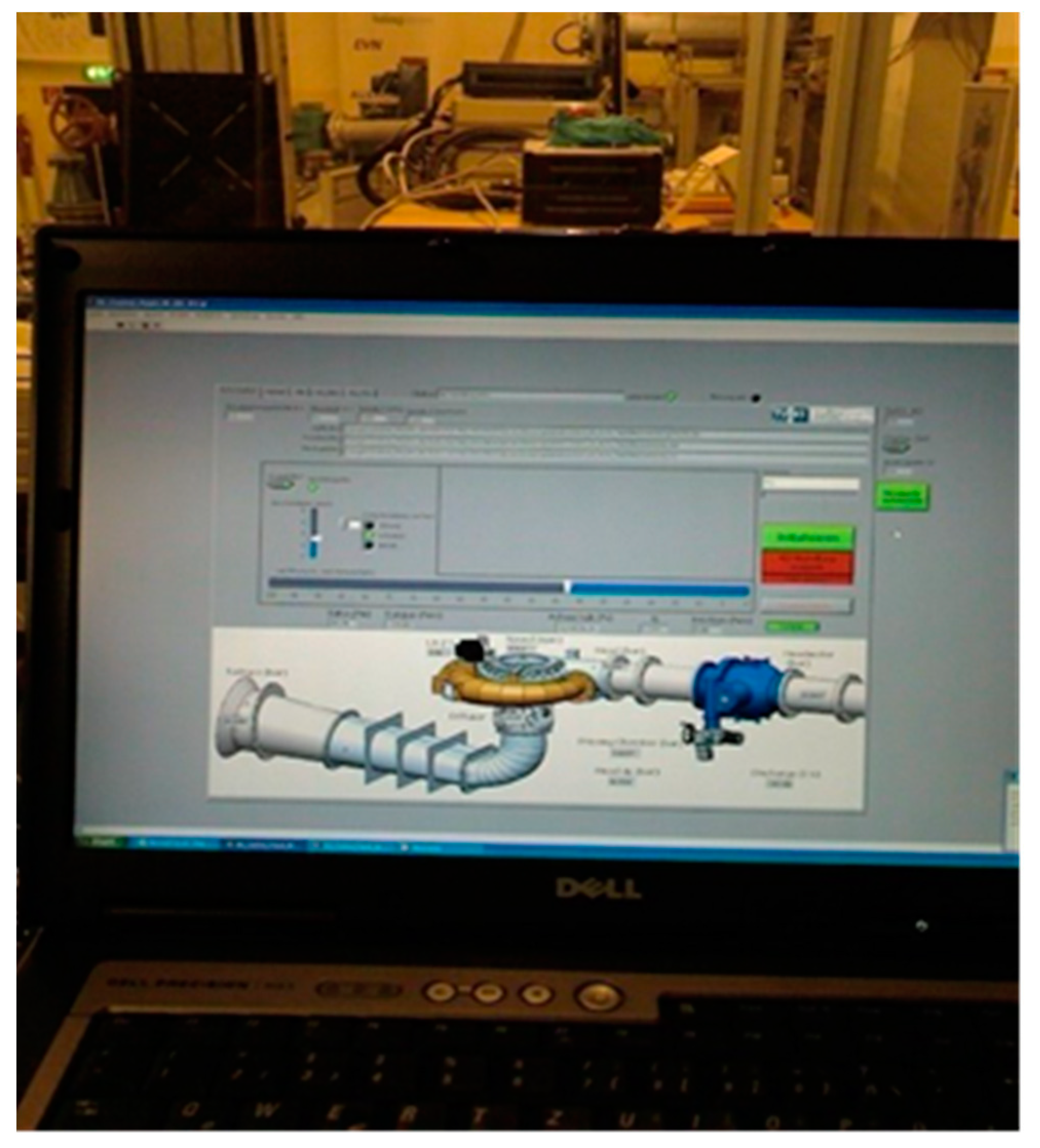
A photograph of Christian Bauer of the Vienna University of Technology, Zdravko Giljen (as a PhD student), and Bernhard List of Voith is presented in Figure 1. Figure 2 shows a photograph taken at the laboratory in Vienna, with a display of the complete pump–turbine installation on the computer. During the test, the laboratory staff did not provide any technical data (e.g., related to what types of equipment were used to obtain the flow rate, head, torque, and so on) to the author; thus, such data are not presented in this paper.
The author also made an official visit to the State Key Laboratory of Water Resources and Hydropower Engineering Science, Wuhan University, China, from 29 February 2016 to 29 March 2016, at the invitation of Yongguang Cheng, director of the laboratory’s Research Section on the Safety of Hydropower Systems. On the test bench, pump–turbines were driven through four-quadrant operations, and the four-quadrant characteristics were tested for two models of pump–turbines under stationary and non-stationary conditions. Measurements were made over the entire area of the four-quadrant diagram: pump mode, braking, turbine mode to the line of runout and continuation in braking mode, reversible pump mode, and start in pump mode. Subsequently, the author analyzed the obtained data, which were made dimensionless for the obtained Suter curves, and then conducted numerical experiments regarding the transient phenomena (1D) in a system with such machines.
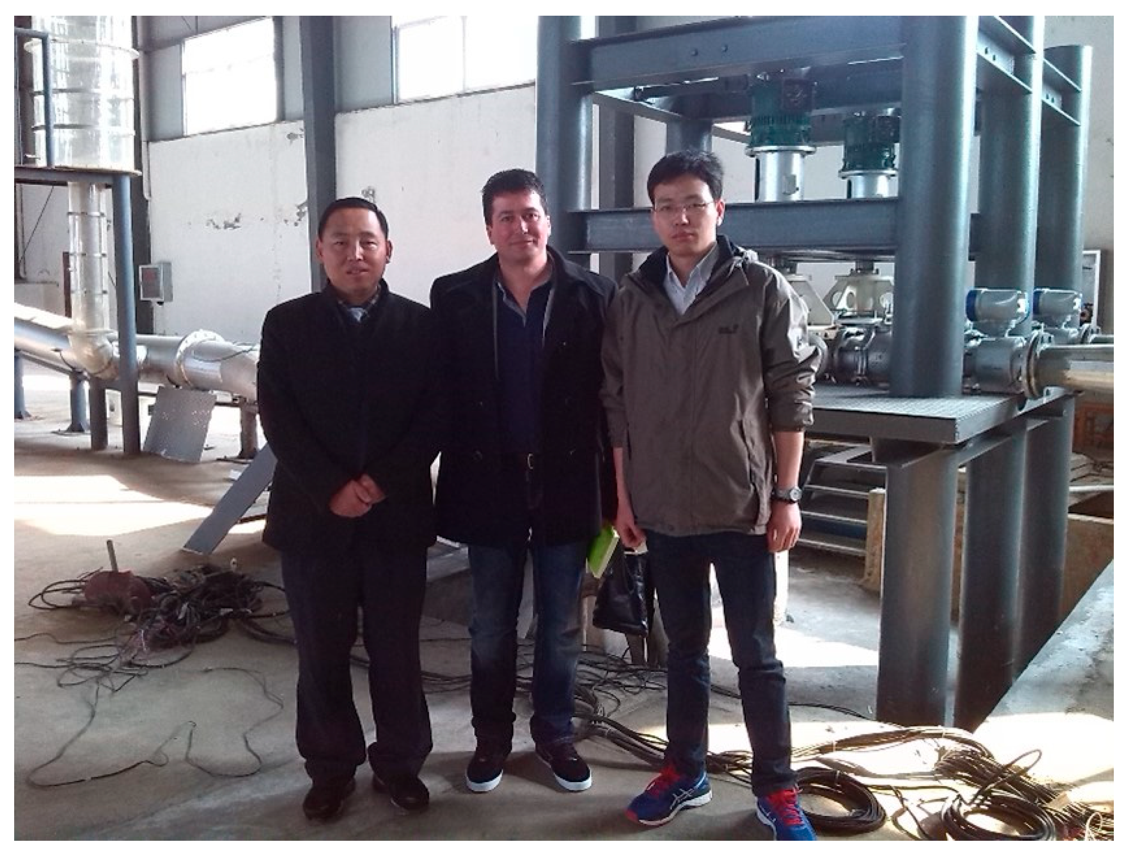
While performing measurements, the author learned how complex the process is in the physical sense during the operation of the pump–turbine in all four modes, as well as how much instability and chaos there is during the transition from pump mode to turbine mode (zone of energy dissipation: discharge, torque, and speed of rotation change sign and direction) and how difficult it is to measure torque, discharge, and speed of rotation in this operating mode. The experimental platform in the laboratory consisted of nine parts: recycled water, excitation protection, speed control, frequency disguise, monitoring, load, measurement, model unit, and diversion system equipment. While developing his doctoral dissertation, the author analyzed the results obtained during the transition process on two pump–turbine models installed in this laboratory, as well as the process of data transformation from four-quadrant pump–turbine characteristic curves to Suter curves. During this period, the author became familiar with the complete installation of two pump–turbines at the State Key Laboratory in Wuhan (upstream reservoir, supply pipeline, upstream branch, installation of two pump–turbine models, downstream branch, surge chamber, downstream pipeline, downstream reservoir), as well as the equipment in the control room, where the data were collected. The process was monitored in the control room while, in the adjacent room, devices were used to process and convert all measurement signals and positions from analog to digital, and the measurements of working points on the four-quadrant characteristic curves in stationary and non-stationary conditions were monitored. The author then analyzed these obtained results. A photograph of Yongguang Cheng and Linsheng Xia of the State Key Laboratory with Zdravko Giljen (as a PhD student) is presented in Figure 3.
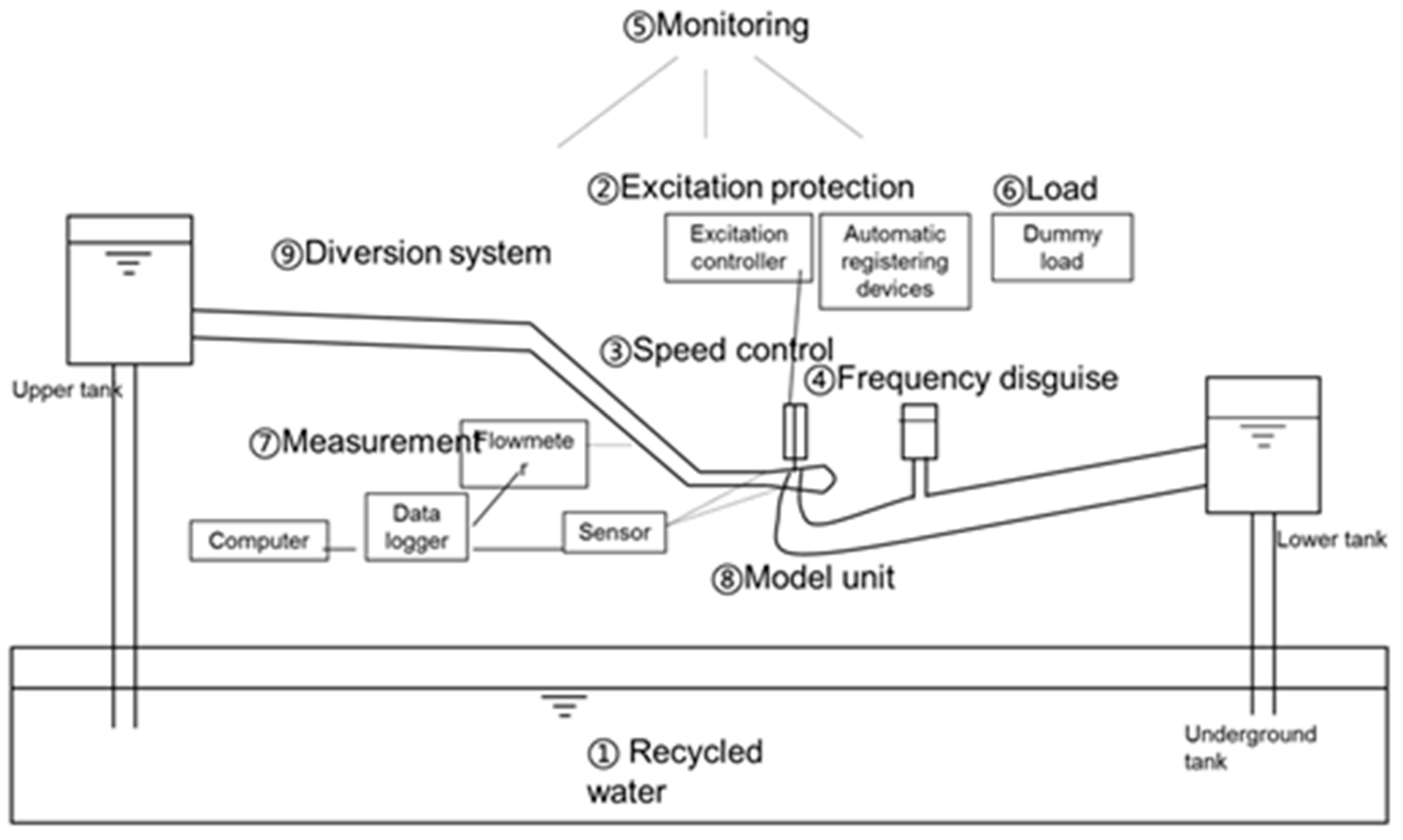
The experimental platform at the laboratory in Wuhan consists of nine parts, as shown in Figure 4: recycled water, excitation protection, speed control, frequency disguise, monitoring, load, measurement, model unit, and diversion system equipment. The recycled water equipment includes cisterns, tanks, backwater channels, pumps, water pipes, valves, electromagnetic flow meters, transformers, distribution equipment, and other auxiliary equipment. Excitation protection equipment includes a generator motor excitation device (generator, automatic registering devices, generator protection devices). The speed control equipment includes a speed controller, tester, digital cylinder actuators, valve controllers, and so on. The frequency disguise equipment includes drive and commutation components. The monitoring equipment includes a local control unit, host computer system, monitoring system software, and industrial TV monitors. The load equipment includes a 4 × 20 kW front-loaded cabinet. The measurement equipment includes a data logger, vibration tester data, and various sensors. The model unit equipment includes four models working as a head pump–turbine and generator motor. The diversion system equipment includes upper/lower reservoirs, inlet/outlet pressure pipelines, a surge chamber, and other components. During this test, the laboratory staff did not provide any technical data on what equipment was used to obtain the flow rate, head, torque, and so on to the author; thus, such data are not presented in this paper.
4. Investigation of Analytical Connection in Data for Working Curves Given in Four Quadrants for 11 Pump–Turbine Models and 2 Pump Models
The authors of this paper conducted data collection, research, and analysis of four-quadrant diagrams for pump–turbine and pump models under different specific speeds nq, then studied and conducted the re-calculation of four-quadrant diagrams for 11 models of pump–turbines into Suter curves. The Suter curve for one pump model (nq = 25 radial pump) was derived from [2] and another model (nq = 41.8 radial pump) from [5]. The authors collected 11 sets of four-quadrant characteristic curves for models of radial pump–turbines (developed in laboratories in China, America, Russia, and Austria), 5 of which were obtained from the State Key Laboratory of Water Resources and Hydropower Engineering Science at Wuhan University and Yongguang Cheng.
From the four-quadrant diagrams for the 11 radial pump–turbine models with nq = 24.34, 24.8, 27, 28.6, 38, 41.6, 41.9, 43.83, 50, 56, and 64.04, the values for the characteristic unit speed of rotation, ; unit discharge, ; and unit moment, were determined, according to four-quadrant curves for various openings of the wicket gates of the conducting apparatus of the 11 models. Then, the authors calculated the degree of efficiency of these curves, and the optimum point with the highest degree of efficiency for the pump and turbine mode was determined for each model, and data for H*, Q*, and M* from the optimal points were taken for the pumping mode and used for further data re-calculation. Then, the authors calculated the values of H, Q, and M for each point on the four-quadrant curves. After this, the values for the dimensionless head, ; dimensionless moment, ; dimensionless speed of rotation, ; and dimensionless discharge variable, were calculated—this refers to the procedure for converting four-quadrant curves to Suter curves. Suter diagrams show the curves of the characteristic head, , and characteristic moment, , expressed as functions of the angle θ, defined by [30].
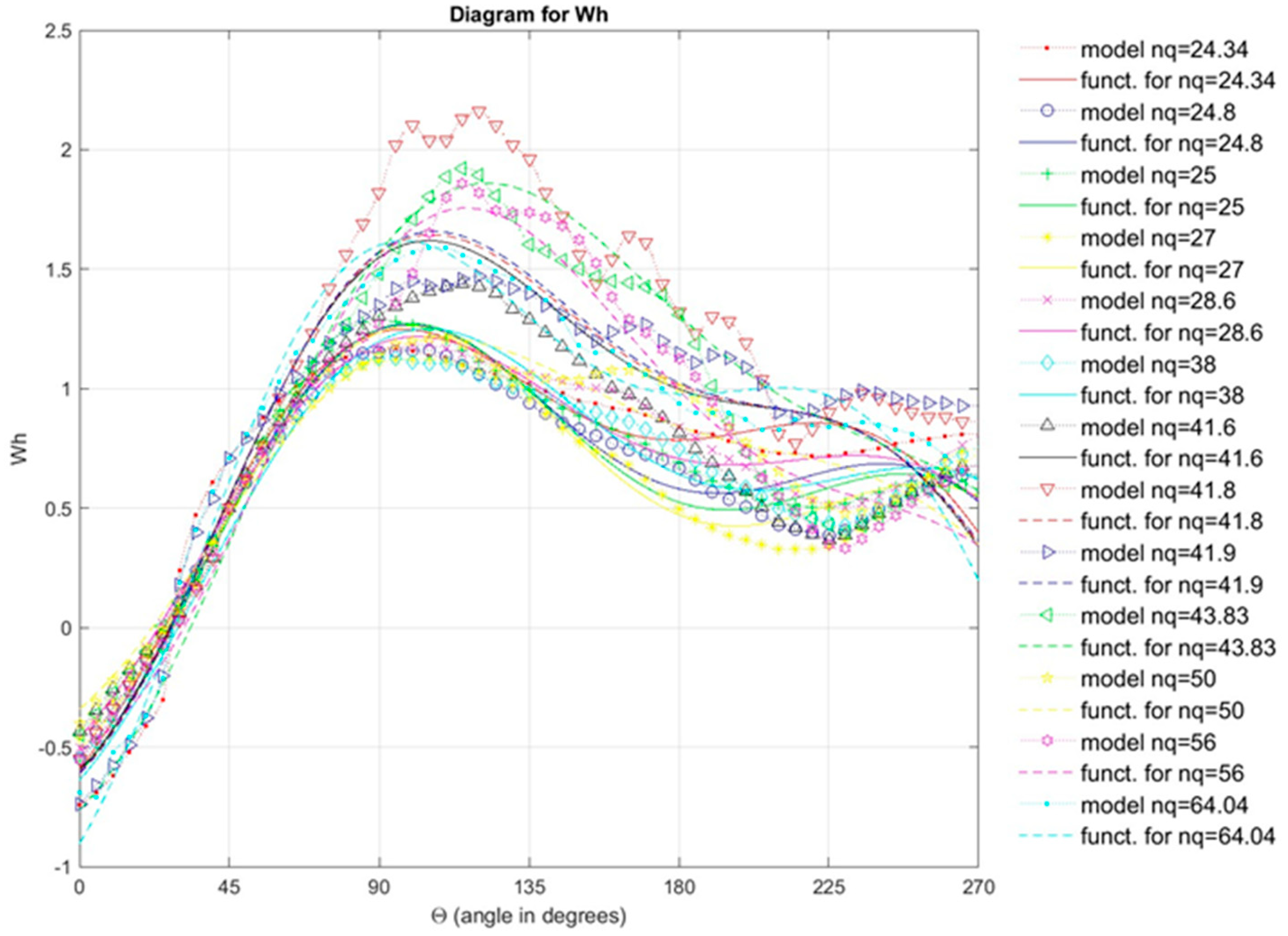
After re-calculating the four-quadrant curves to Suter curves for all openings of wicket gates of the conducting apparatus for the 11 radial pump–turbine models, as shown in single diagrams in Figure 5 and Figure 6, Suter curves for the optimal opening of the wicket gates of the conducting apparatus for one model of the radial pump (nq = 25) were derived from [2], and those for another radial pump model (nq = 41.8) were derived from [5].
The parameters of the various pump–turbines are as follows: China: nq = 24.34, opening 24 mm; USA (Bad Creek): nq = 24.8, opening 26 mm; Serbia (Bajina Basta): nq = 27, opening 24 mm; USA: nq = 28.6, opening 18°; China: nq = 38, opening 24°; Vienna, Austria: nq = 41.6, opening 36 mm; China: nq = 41.9, opening 20°; Russa: nq = 43.83, opening 28 mm; China: nq = 50, opening 20.03°; China: nq = 56, 40 mm; and Russia: nq = 64.04, opening 16 mm.
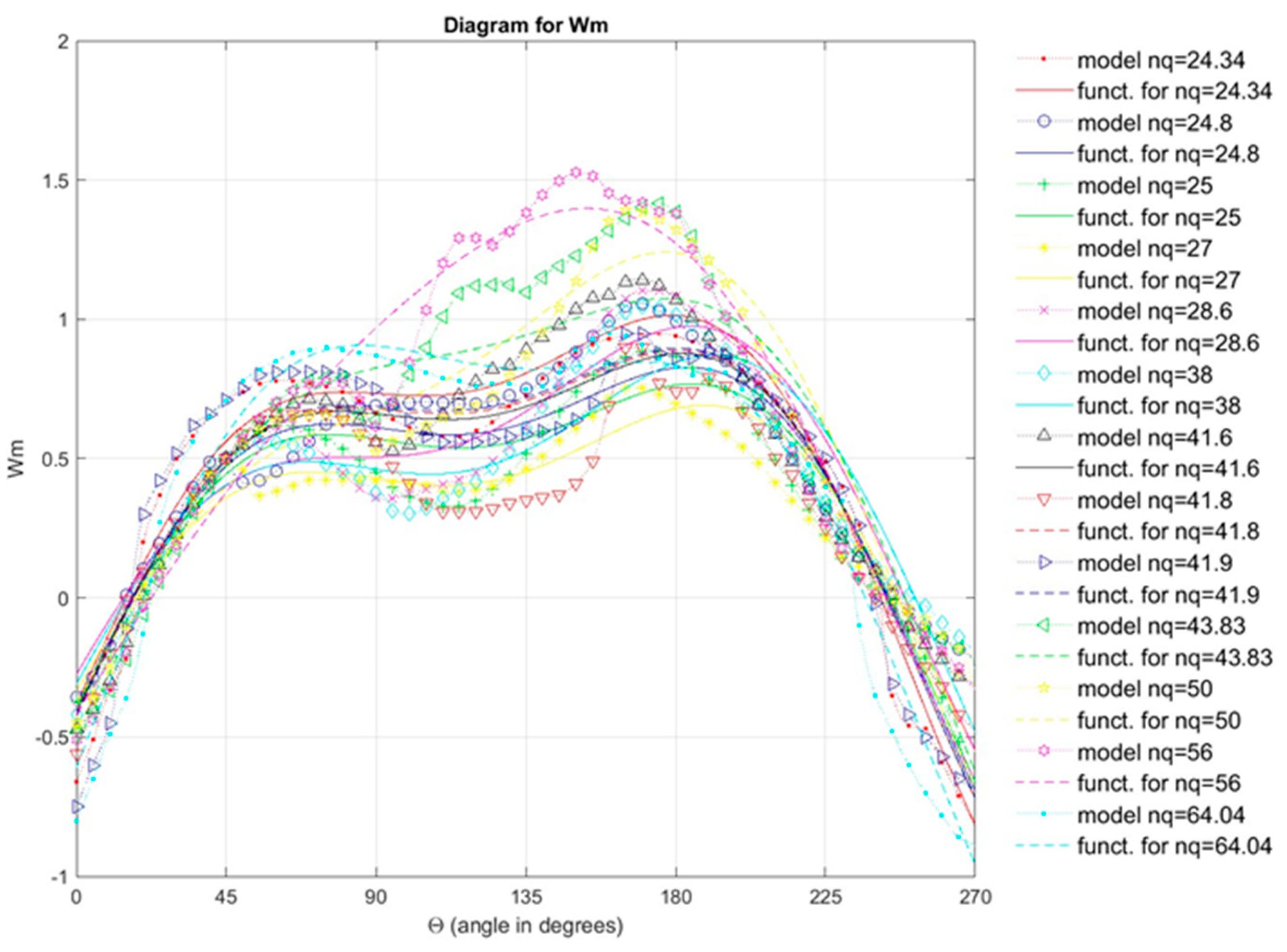
Figure 5 and Figure 6 show diagrams with 13 Suter curves for the Wh and Wm characteristics, of which 11 are for pump–turbine models and 2 are for pump models. According to a detailed analysis of the structure of the curves, the authors concluded that, in the following steps, they should observe Suter curves for pump–turbines and pumps together. Based on this, universal equations for the Wh and Wm characteristics could be obtained from a numerical model developed in MATLAB. A variant of this numerical model is detailed below (regression procedure: least squares method; interpolation procedure: spline method) [31], and the obtained results are shown in various diagrams.
4.1. Details of the Procedure and Variants
The aim of this study was to analyze the four-quadrant operating characteristics (Q11, n11, M11), with the idea of determining whether a law exists. It is well known that the operating curves (Q11, n11, M11) are stable in pump mode and turbine mode, and data for those regimes have been studied in more detail than data for the complete four-quadrant characteristic curves.
The authors of this paper, based on the data of Suter curves for 11 pump–turbine models—along with the data for one pump model from [5] and another pump model from [2]—used MATLAB to develop a numerical model using polynomial regression to obtain universal equations for the Wh and Wm characteristics, in order to analyze the existence of a more general law for the obtained curves depending on the specific speed nq. The process of developing the model consisted of the following steps.
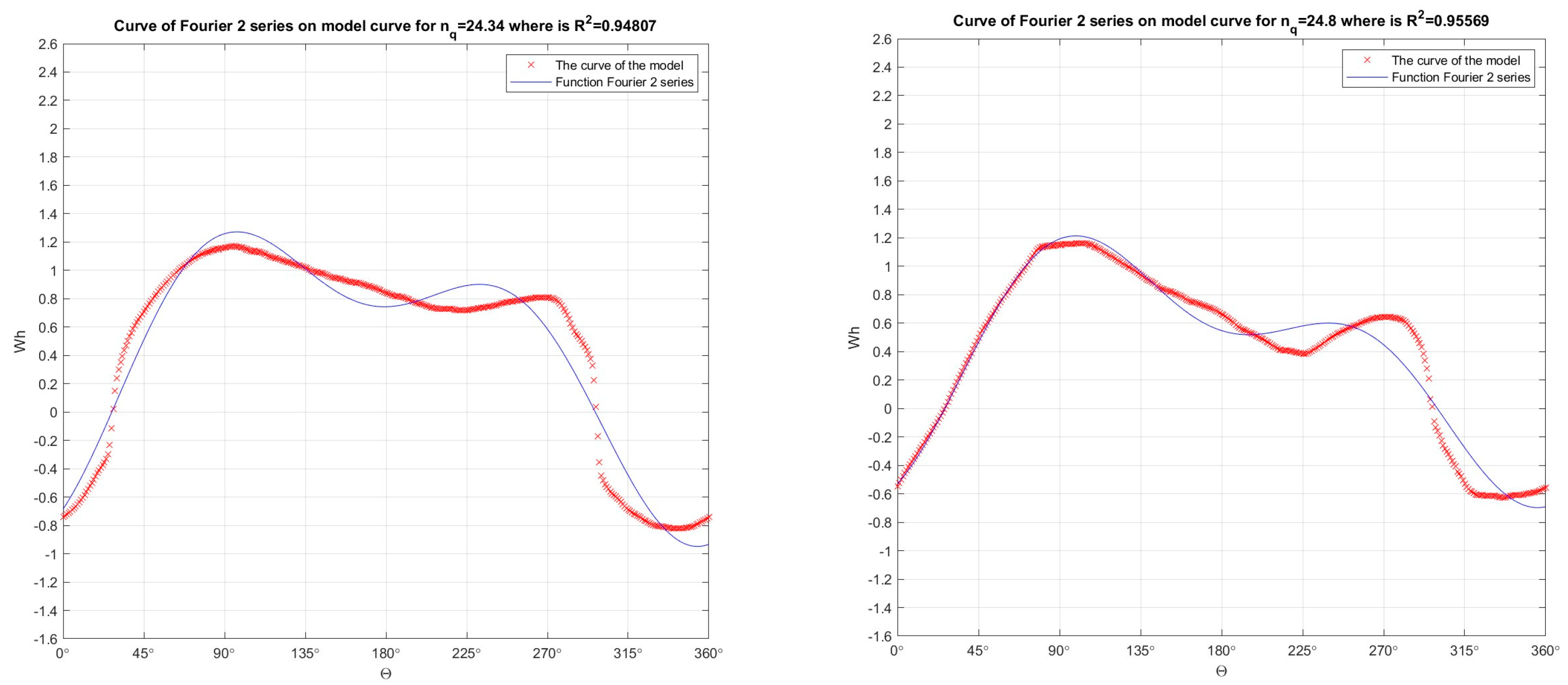
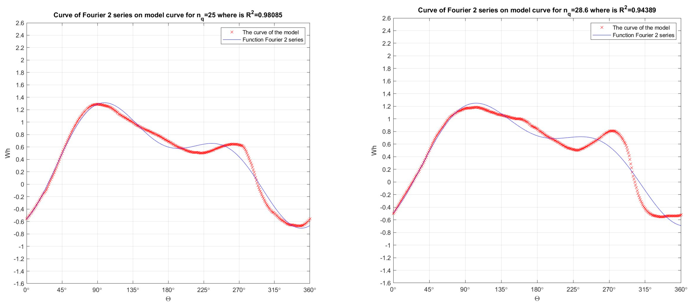
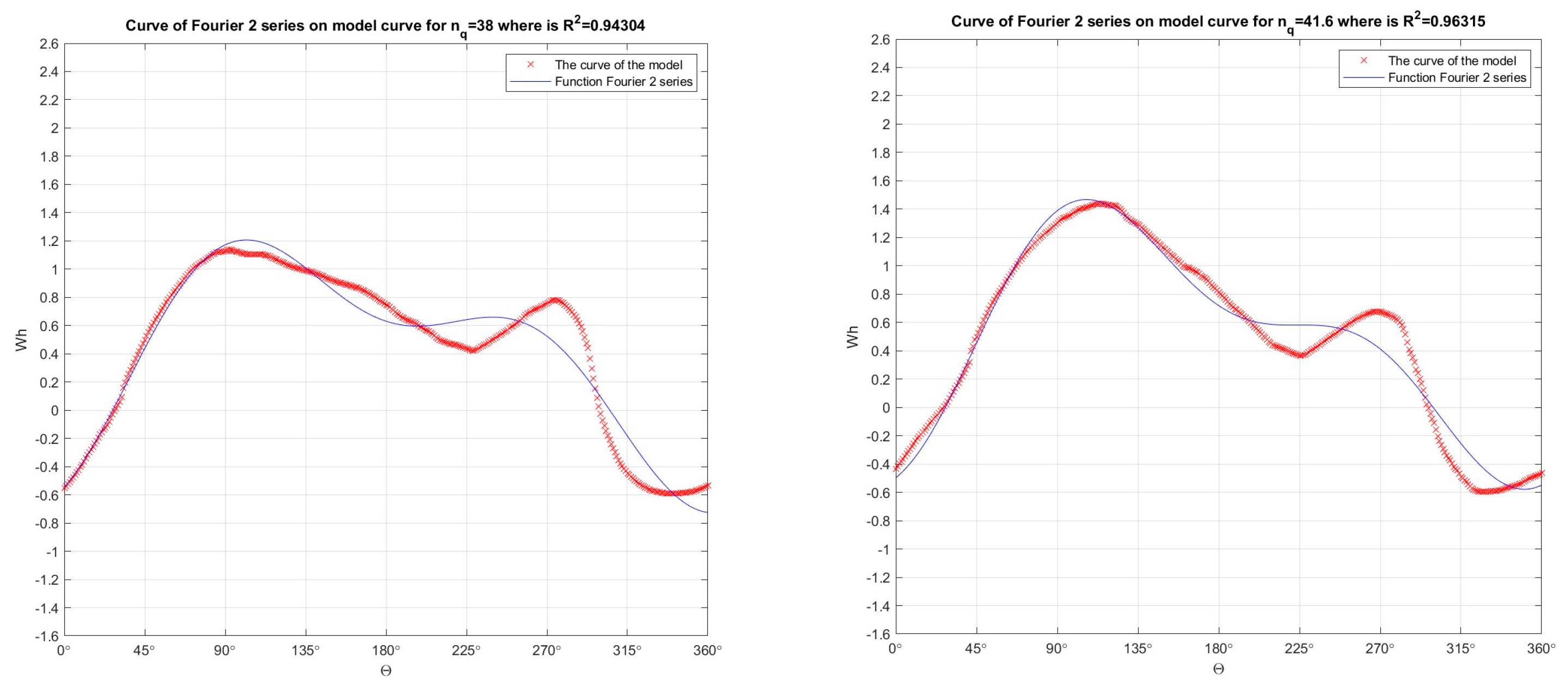
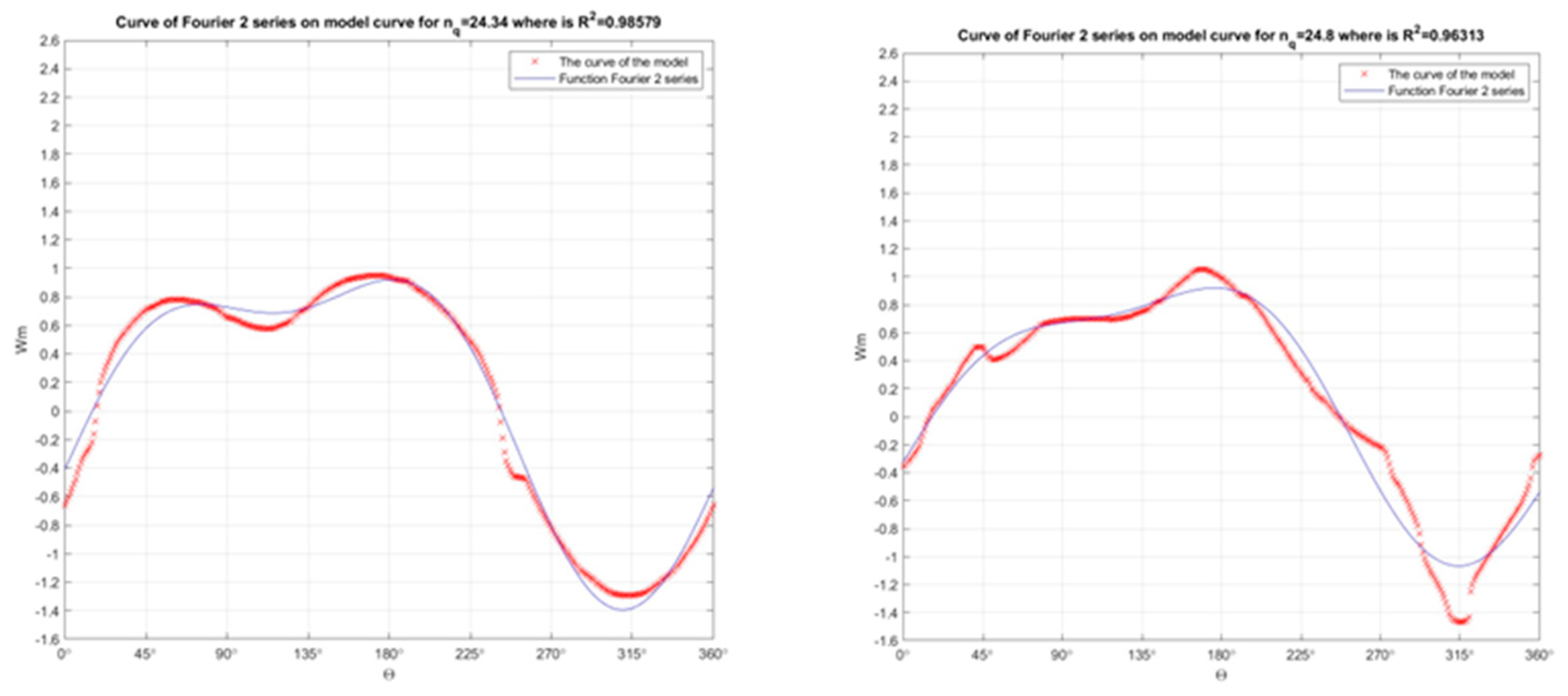
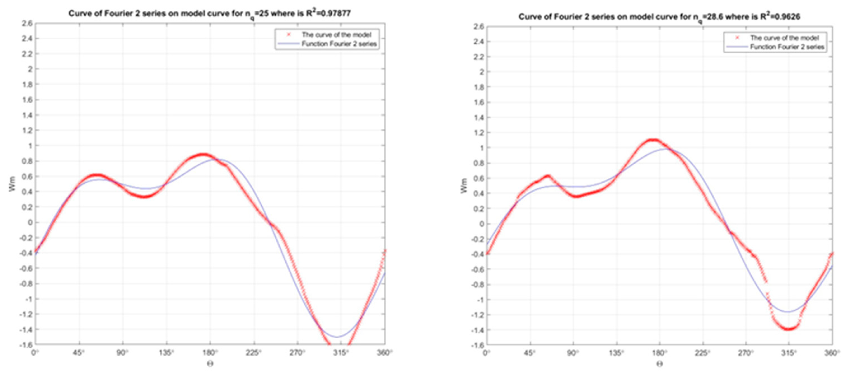
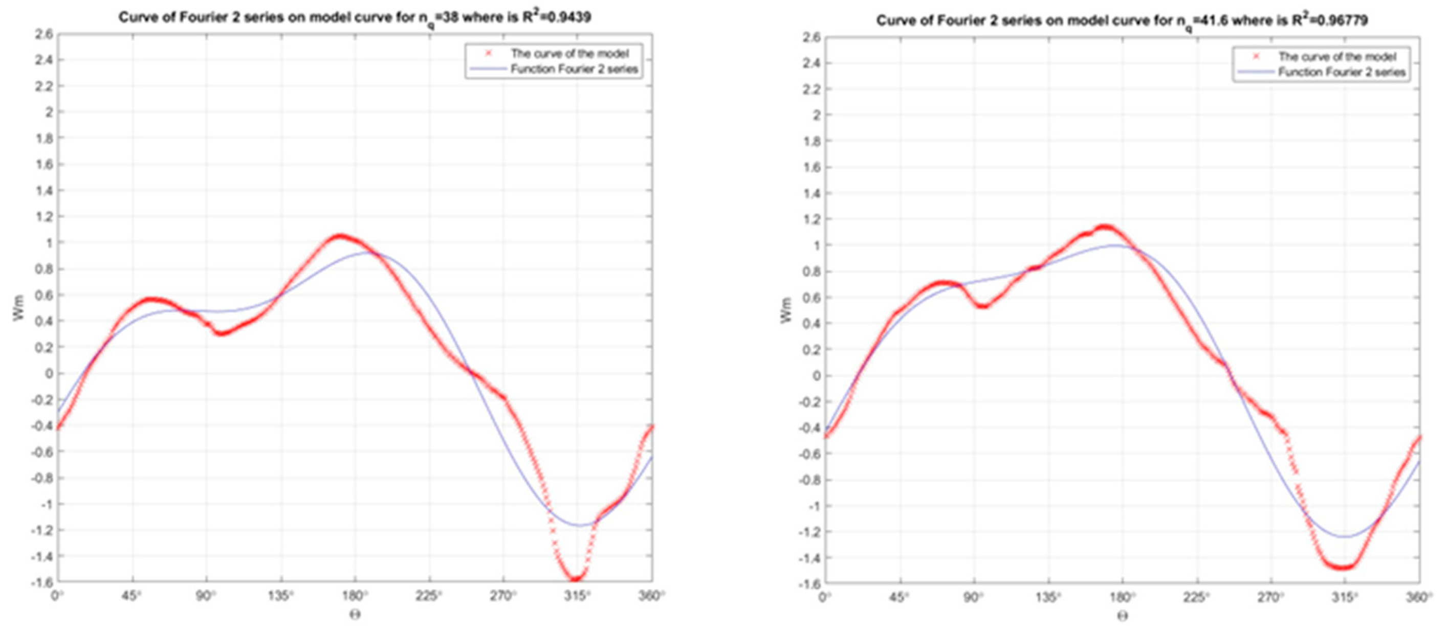
Step one: All 13 Suter curves (each curve separately for both the Wh and Wm characteristics) for 11 pump–turbine models and 2 pump models with theta ranging from 0° to 360° were passed through the second-order Fourier function, as shown in Figure 7, Figure 8 and Figure 9 for Wh and Figure 10, Figure 11 and Figure 12 for Wm. Diagrams for all Suter curves passed through the Fourier function are not shown in order to not overload this paper with a large number of diagrams; instead, diagrams for six Suter curves (with nq = 24.34, 24.8, 25, 28.6, 38, and 1.6) regarding the Wh and Wm characteristics are shown.
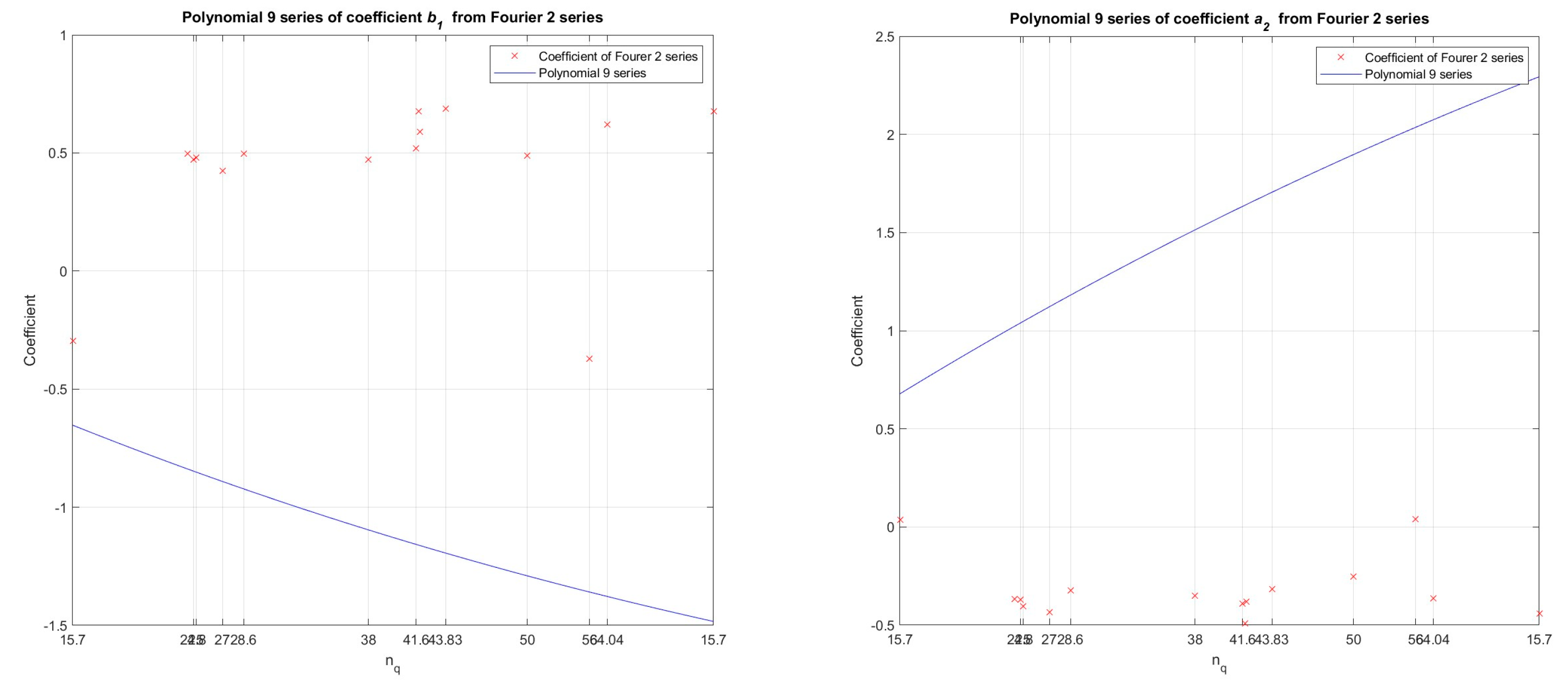
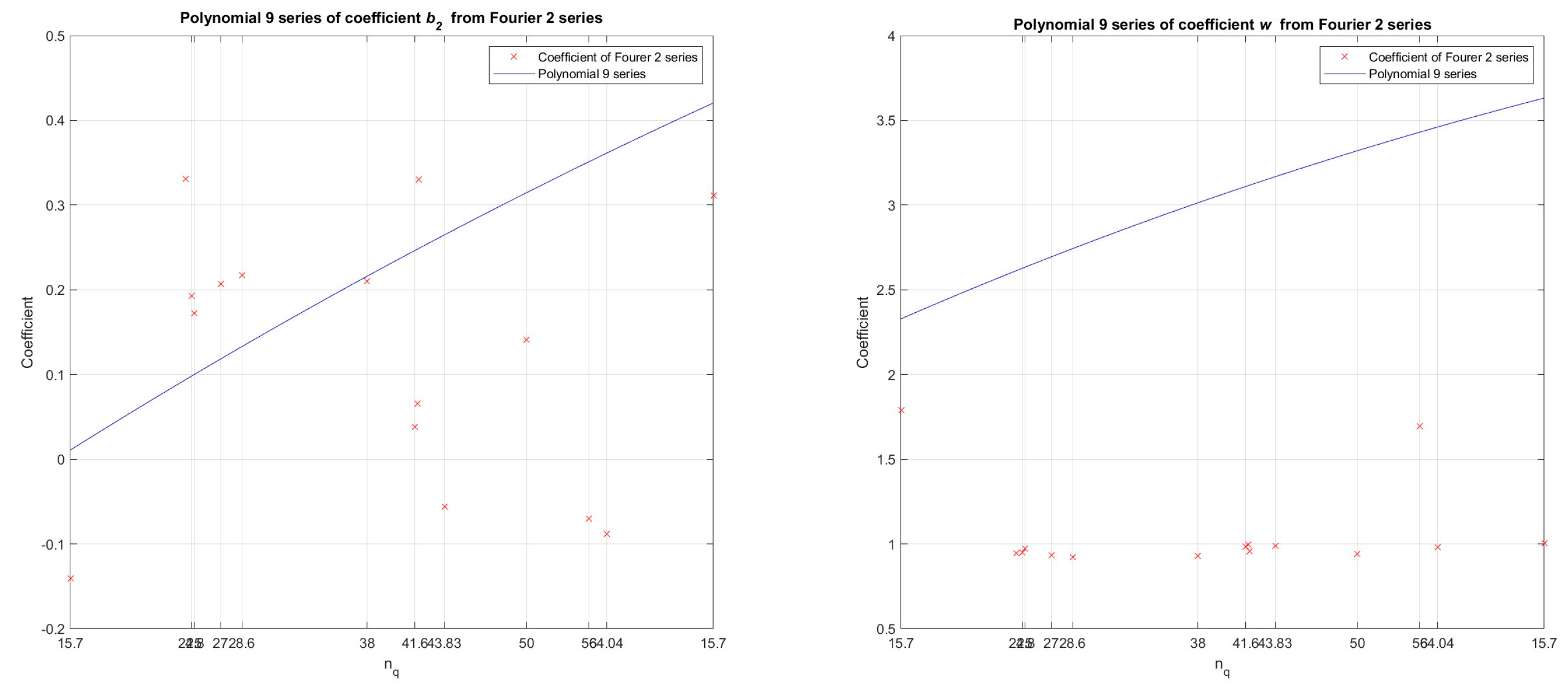
Step two: The coefficients a0, a1, a2, b1, b2, and w were taken from the 13 second-order Fourier functions through which the 13 Suter curves were passed (11 pump–turbine models and 2 pump models) separately for the Wh and Wm characteristics of each curve. Then, the values for these coefficients were grouped on separate diagrams. The diagrams for Wh are shown in Figure 13, Figure 14 and Figure 15, and those for Wm in Figure 16, Figure 17 and Figure 18, where the values of the coefficients from the second-order Fourier functions are shown depending on the specific speed nq. A polynomial of order 9 was passed through the values of the coefficients listed on these diagrams, and each polynomial shows the dependence of the coefficients on the specific speed nq.
Step 3: The dependence between the values of the coefficients (a0, a1, a2, b1, b2, w) and the specific speed nq (for 11 pump–turbine models and 2 pump models) was determined by polynomial regression (using the polynomial of order 9) through the numerical model developed in MATLAB.
Step 4: Based on the developed numerical model, universal equations for the Wh and Wm characteristics were obtained depending on the specific speed. These universal equations were expressed in the numerical model with the second-order Fourier equation, depending on the specific speed.
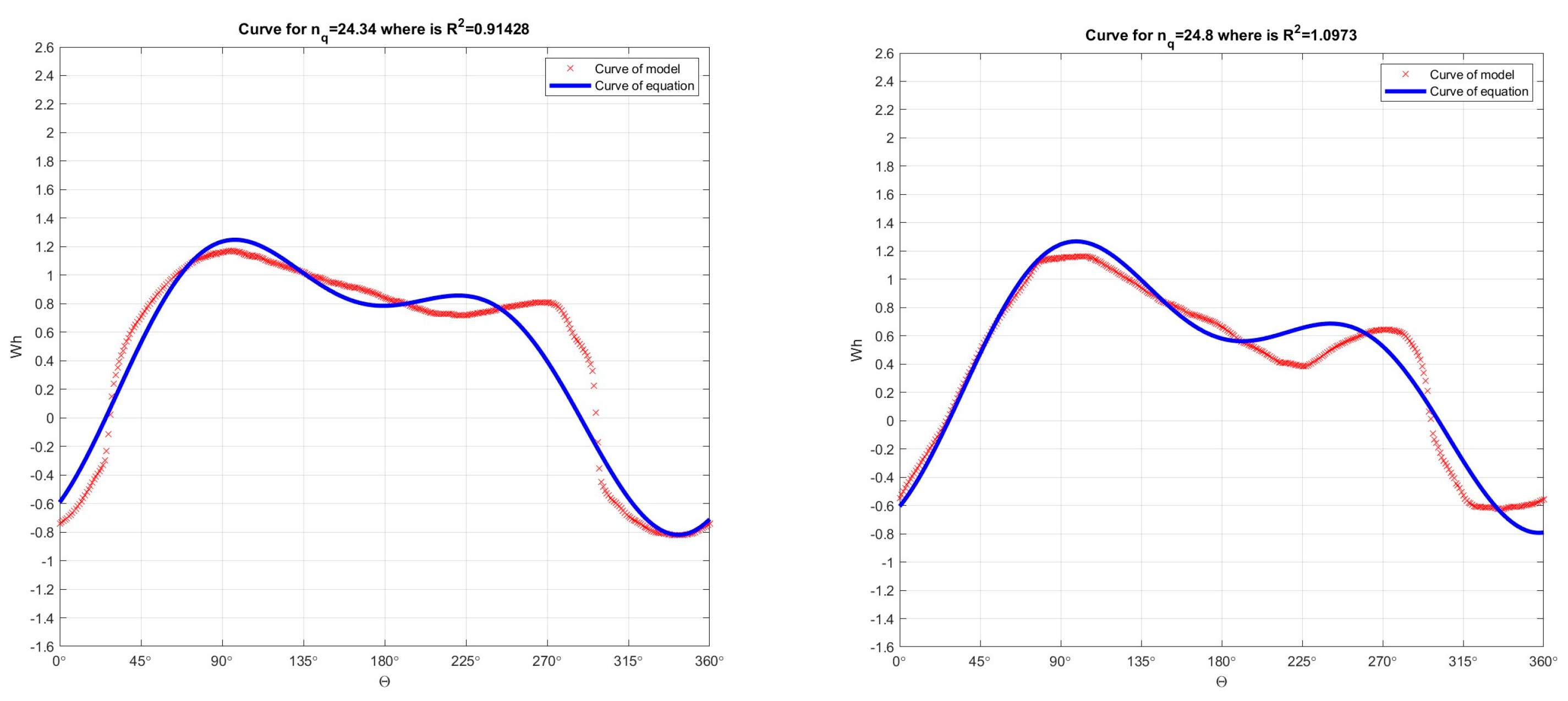
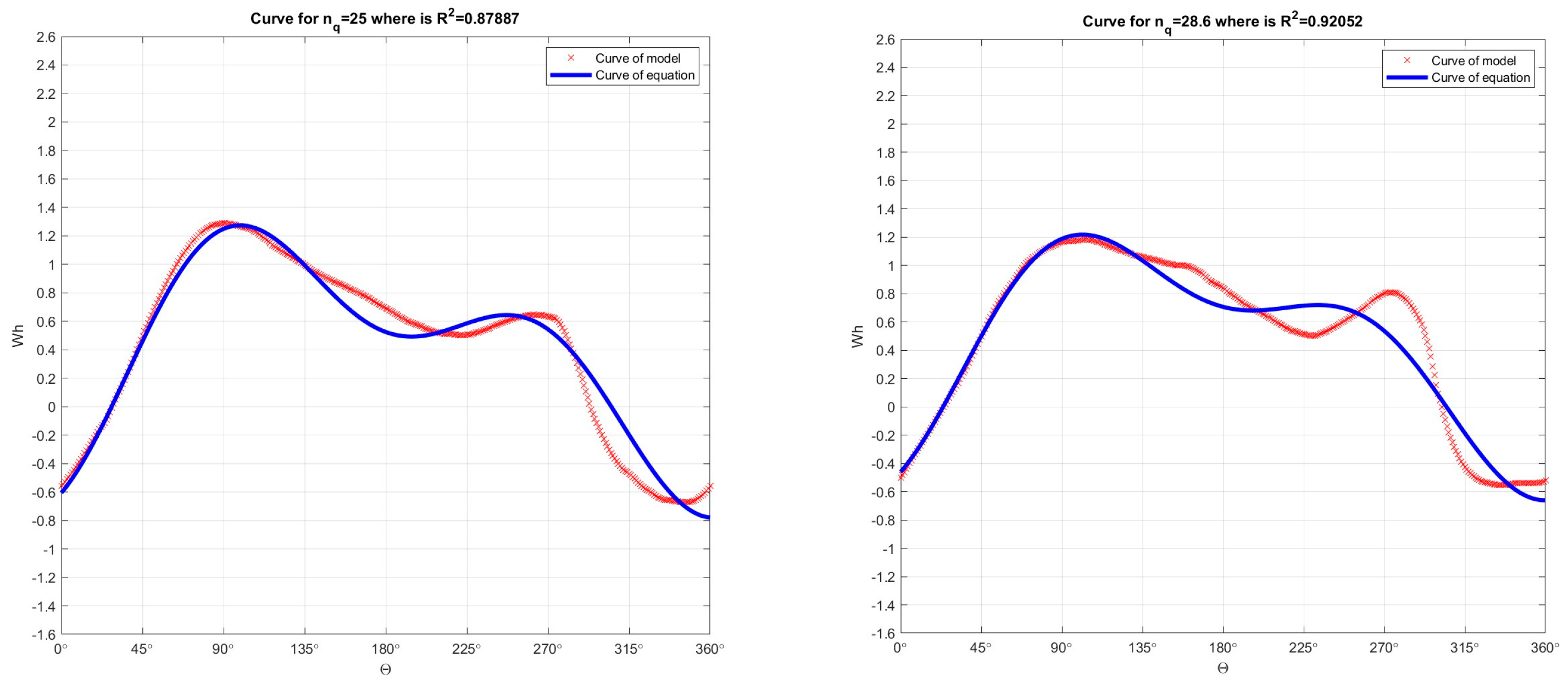
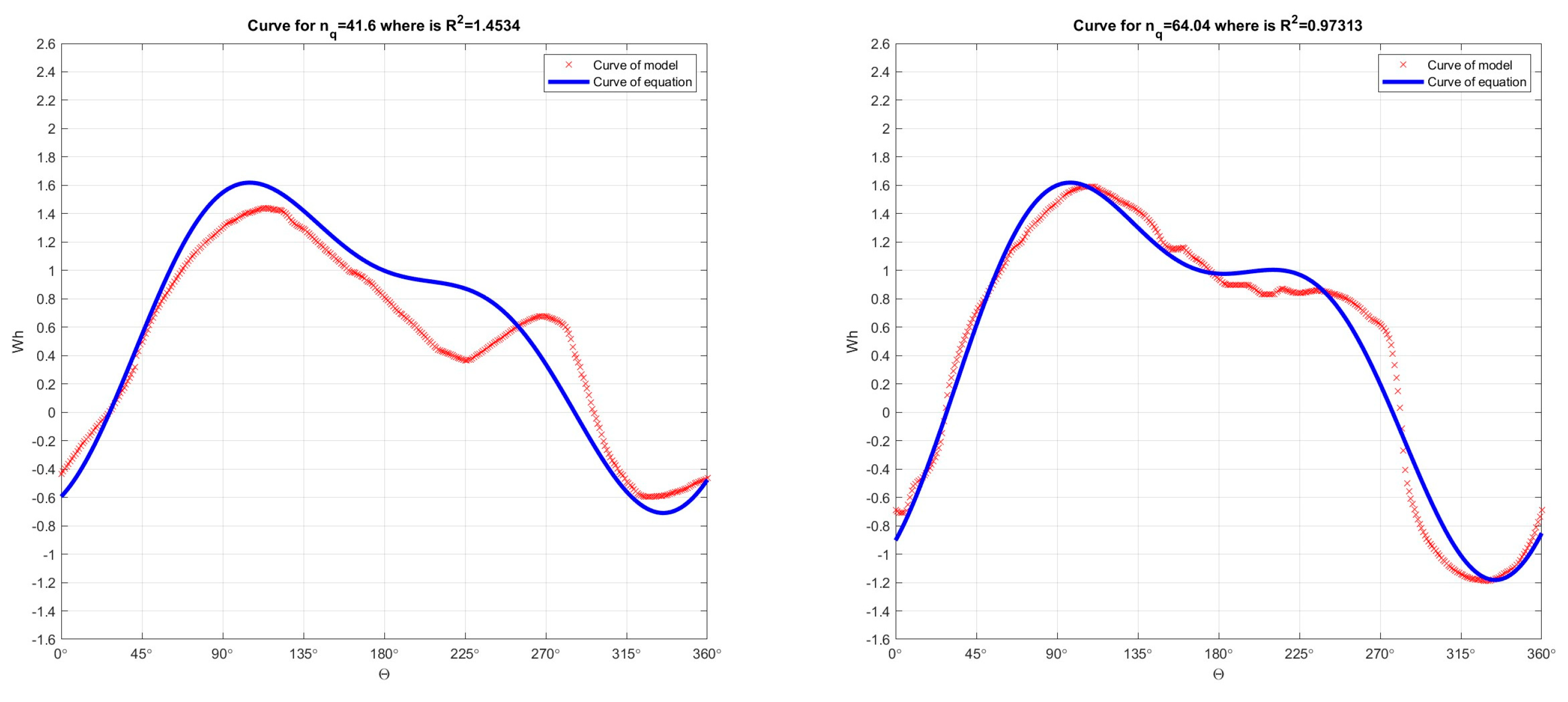
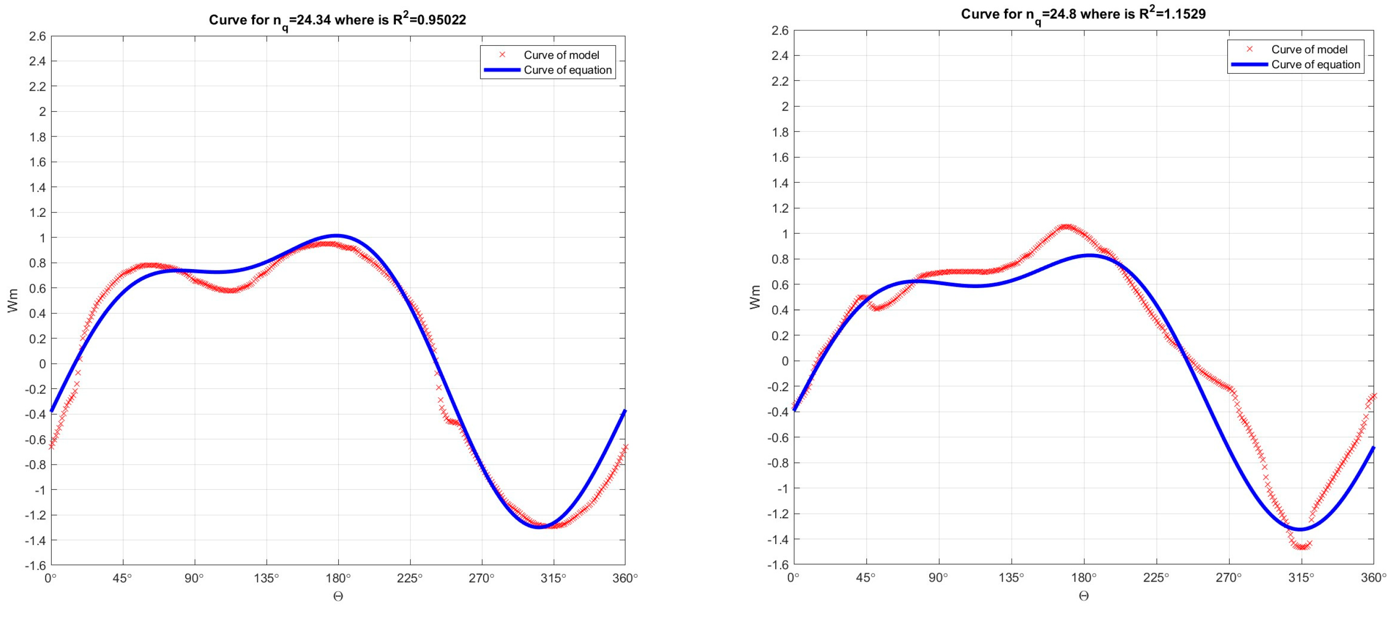
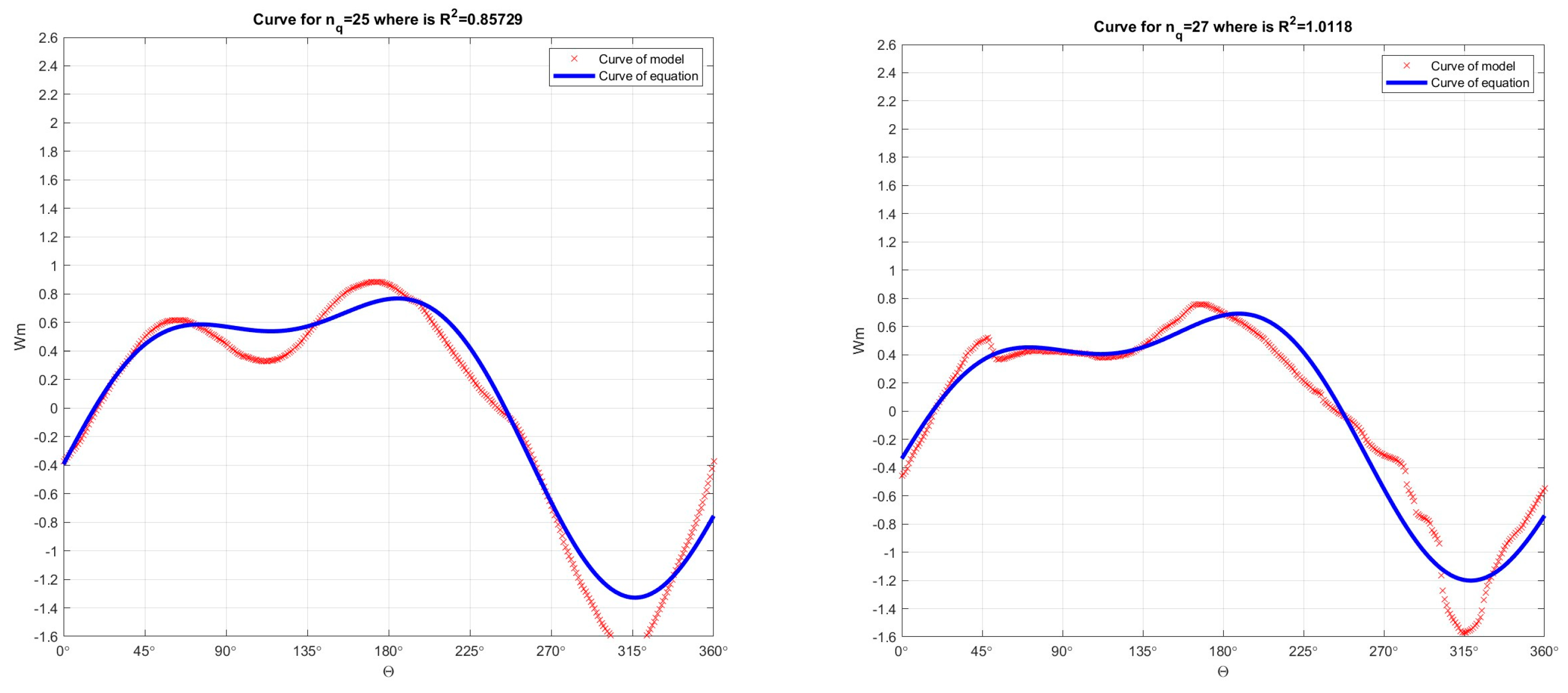
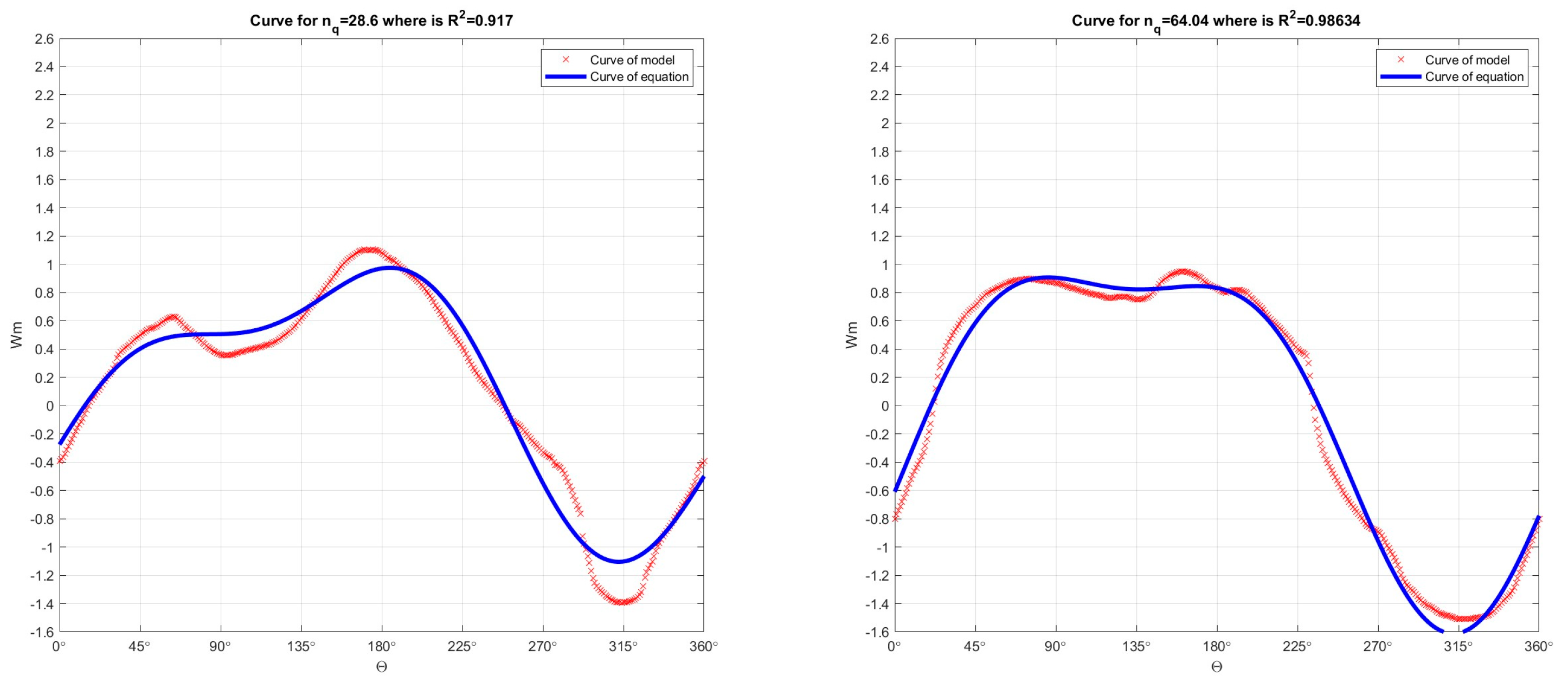
Step 5: Based on the developed numerical model, from the universal equations, the authors obtained values for the Wh and Wm characteristics for 13 Suter curves at different specific speeds nq and compared them with the values for the Wh and Wm characteristics in the 13 Suter curves obtained by re-calculating the model curves with different specific speeds nq (for the 11 pump–turbine models and 2 pump models). In particular, the authors compared the Suter curves for the Wh and Wm characteristics with those obtained through re-calculation of the Suter curves obtained from the universal equations. In order to not overload this paper with a large number of diagrams, diagrams for six Suter curves are presented in Figure 19, Figure 20 and Figure 21 for the Wh characteristic and six in Figure 22, Figure 23 and Figure 24 for the Wm characteristic (nq = 24.34, 24.8, 25, 27, 28.6, and 64.04). Figure 5 and Figure 6 show the Suter curves for the Wh and Wm characteristics, respectively, obtained from the re-calculated model and from the universal equation (for 11 pump–turbine models and 2 pump models).
MATLAB was used to develop a numerical model for calculating the transient processes in a pumping plant where two pumps are installed (using the method of characteristics; MOC). As input data for this numerical model, the authors used the Suter curves for the Wh and Wm characteristics, which were obtained by re-calculating the model curves Q11, n11, M11 for different values of the specific speed, as well as the Suter curves for the Wh and Wm characteristics obtained from universal equations under various specific speed values.
In order to more reliably and precisely unite all values from the experimental four-quadrant curves for different values of nq in the universal equation for the Wh and Wm characteristics, we utilized a fitting method. The focus of this paper is on the simple derivation and practical application of equations for data fitting, and we should be aware that there are theoretical aspects of regression that are of practical importance. For example, some statistical assumptions are inherent in the linear least squares procedure: each x has a fixed value, is not random, and is known without error; the y values are independent random variables, and all have the same variance; and y values for a given x must be normally distributed. As polynomial regression in MATLAB is applied in this paper, the authors developed a numerical model for performing polynomial regression on a large set of points on four-quadrant curves of pump and pump–turbine models under different values of nq. The least squares criterion can easily be extended to fitting data up to higher-order polynomials. For example, in this paper, the authors fit the experimental data from four-quadrant curve pumps and pump–turbines using a ninth-order polynomial, which gave very good results; this is why the authors decided to use this fitting method. For this case, we see that the problem of determining the least squares regression of polynomials of the ninth order is equivalent to solving a system of 10 simultaneous linear equations. This analysis can be easily extended to a more general case. In this way, we recognize that determining the coefficients of an m-order polynomial is equivalent to solving a system of m + 1 simultaneous linear equations.
As can be clearly seen from Figure 7, Figure 8, Figure 9, Figure 10, Figure 11 and Figure 12, some coefficients of determination R2 were not ideal and some localized error results were large; in the following part, we give recommendations and measures to address this issue. In this paper, the second-order Fourier function was used for passing through the Suter curves (obtained by re-calculating the model curves Q11, n11, M11) under different nq, and the values of coefficient of determination R2 were not ideal. During the development of this paper, we trialed many different types of functions (Fourier functions of order 2, 3, 4, 5, 6, 7, and 8; polynomials of order 1, 2, 3, 4, 5, 6, 7, 8, and 9; and Gaussian functions of order 1, 2, 3, 4, and 5) and many combinations of these functions. We also performed many analyses for all values of the coefficient of determination R2 for all combinations of functions, and the best results were obtained with the combination of the second-order Fourier function and polynomial of order 9, which is why the values obtained with these two functions are presented. The authors recommend that researchers who would like to conduct further research in this area analyze other mathematical tools that can enhance the fitting process and obtain better values for the coefficient of determination R2. All of the above explains why the polynomial regression (with polynomials of order 9) did not work well, and why we chose a fit with higher accuracy for the coefficients of the second-order Fourier function. This also explains why the polynomial curves in Figure 13, Figure 14, Figure 15, Figure 16, Figure 17 and Figure 18 appear to be far from the samples. The results presented in this paper represent the maximum reached during the process of researching these issues, which was conducted over the past few years. It is encouraging that, while there were some deviations (according to the diagrams for some coefficients and R2 values), this does not mean the approximations of Wh and Wm are bad in the engineering sense, as these coefficients have very little effect on the final parameters being investigated. According to our assessment, the error was about 3%, which is not of great importance in engineering practice. The final conclusion is that the calculation method provided at the end of this paper with the comparison diagrams is proof that, even with larger deviations of some coefficients, the transient calculation results remain very similar.
4.2. Universal Equation for Wh Characteristic Depending on nq Obtained from the Developed Numerical Model in MATLAB with Second-Order Fourier Function
The universal equation for the Wh characteristic was obtained from the numerical model developed in MATLAB, presented in the form:
Wh, = f(nq,θ).
The universal equation for the Wh characteristic with respect to the second-order Fourier function is as follows:
The coefficients in the universal equation are expressed using polynomials of order 9:
The values of the coefficients in the universal equation for the Wh characteristic, obtained from the numerical model developed in MATLAB based on the procedure described in this paper, are listed in Table 1.
4.3. Universal Equation for Wm Characteristic Depending on nq Obtained from the Developed Numerical Model in MATLAB with Second-Order Fourier Function
The universal equation for the Wm characteristic obtained from the numerical model developed in MATLAB is presented in the form:
Wm = f(nq,θ).
The universal equation with respect to the second-order Fourier function is as follows:
The coefficients in the universal equation for the Wm characteristic are expressed using polynomials of order 9:
The values of the coefficients in the universal equation for the Wm characteristic obtained from the numerical model developed in MATLAB based on the procedure described in this paper are listed in Table 2.
5. Application of Universal Equations for Wh and Wm for Calculation of Transient Processes in Radial Hydraulic Machinery
For validation purposes, we consider a pumping plant in which two pumps are installed. The complete technical data of the plant are listed in Table 3, and a schematic representation is shown in Figure 25. The data for the pumping station were taken from [3]. The transient processes taking place in the pumping plant during load rejection of pumps were calculated using a numerical model developed by the authors in MATLAB.
As input data for the numerical model, we used the Suter curves for the Wh and Wm characteristics obtained by re-calculating the model curves Q11, n11, M11 and the Suter curves obtained from universal equations for different values of the specific speed nq (11 radial pump–turbine models with nq = 24.34, 24.8, 27, 28.6, 38, 41.6, 41.9, 43.83, 50, 56, and 64.04; and two radial pump models with nq = 25 and 41.8).
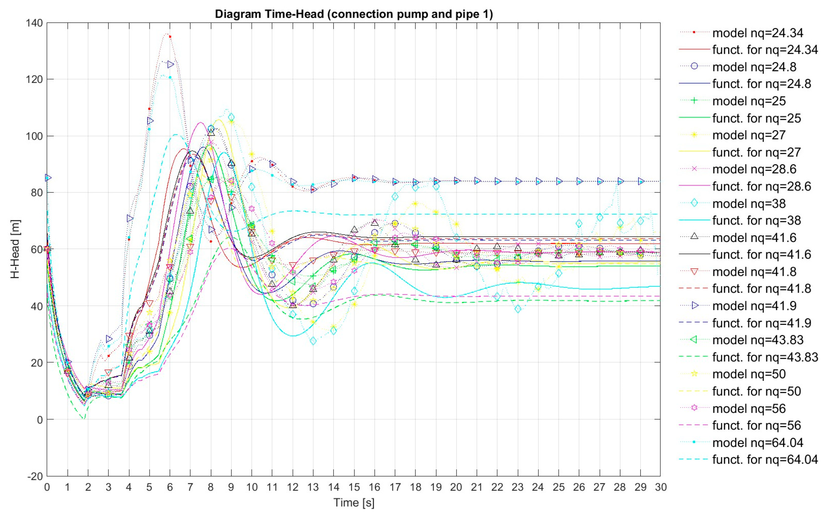
The transient process calculation results are presented visually in Figure 26, Figure 27 and Figure 28. These diagrams show the changes in head, discharge, and speed of rotation during transient processes in the pump station (connection pump and pipe 1), and comparisons of the obtained results under the 13 specific speeds nq.
From Figure 26, it can be seen that the pressure drop at the connection between the pump and pipeline 1 occurred 2 s after the start of the transient process and, for all 13 speeds, this minimum pressure had approximately the same value (around 6 m.w.c.). Meanwhile, the maximum pressure occurred between 5 and 11 s after the beginning of the transient process. The maximum pressure value at the connection between the pump and pipeline 1 differed under the 13 speeds, varying in the range of 80 to 138 m.w.c. This clearly indicates the influence of the specific speed nq on the change in pressure at the connection. One of the main objectives of this work is to demonstrate the influence that the specific speed has on the transient process at the pump station.
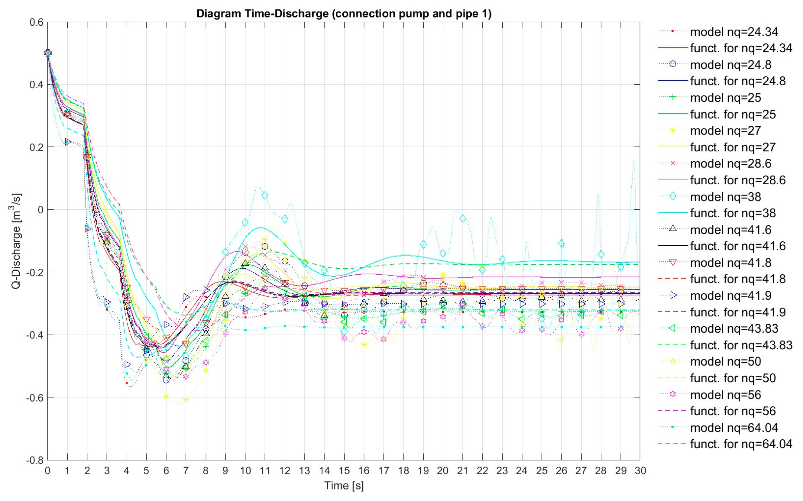
Figure 27 shows the change in discharge during the transient process at the pump station (connection pump and pipe 1), comparing the obtained results for 13 specific speeds.
From Figure 27, it can be seen that the discharge drop at the connection between the pump and pipeline 1 occurred between 4 and 8 s after the beginning of the transient process. In that time interval, the discharge had the lowest value and was approximately the same for all 13 specific speeds, around −0.55 m3/s. The maximum discharge occurred between 9 and 13 s after the beginning of the transient process and the values under the 13 specific speeds varied in the range of −0.38 to 0.11 m3/s, which clearly indicates the influence of the specific speed nq on the change in discharge at the connection between the pump and pipeline 1.
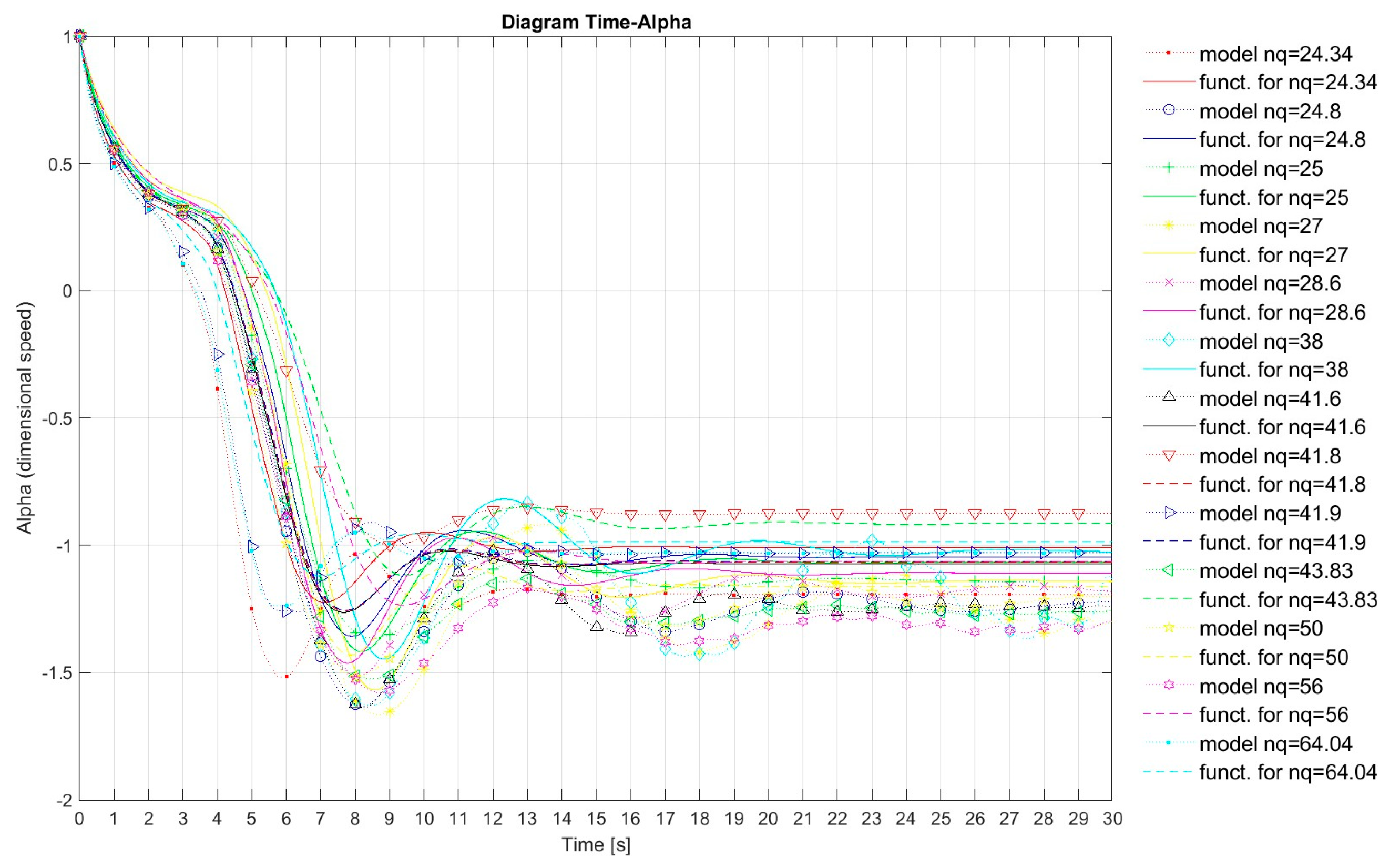
The diagram presented in Figure 28 shows the change in dimensionless speed during the transient process of the pump, comparing the results obtained for the 13 specific speeds. It can be seen that the drop in rotation speed of the pump occurred between 5.5 and 9.0 s after the beginning of the transient process. In this time interval, the speed of rotation had the lowest value, and the minimum value for the 13 specific speeds varied in the range of −1.2 to −1.80 (dimensionless speed). The maximum speed of rotation occurred between 9.5 and 14 s after the beginning of the transient process, and the value for the 13 specific speeds varied in the range of −1.1 to −0.8 (dimensionless speed). This clearly indicates the influence of specific speed on the change in speed of rotation at the pump during the transient process at the pump station.
6. Conclusions
Universal equations for the Wh and Wm characteristics depending on the specific speed nq were obtained for the first time, through the use of a numerical model developed in MATLAB. The final expressions of the equations, as well as the model used to obtain them, were developed by the authors using the second-order Fourier function to fit the data.
Comparisons of the results obtained when calculating the transient process at a pumping plant under 13 specific speeds are shown in Figure 26, Figure 27 and Figure 28. For each of the 13 specific speeds, the values for the Suter curves for the Wh and Wm characteristics were obtained by re-calculating the model characteristics Q11, n11, M11, and from the universal equations for the Wh and Wm characteristics. Then, the data for the Suter curves were used as input data for the numerical model in order to calculate the transient process at this pump station. In the first case, the set of points for the measured diagram was entered as a separate file outside the numerical model developed in MATLAB. In the second case, the values obtained from the universal equations for the Wh and Wm characteristics were entered (these equations are included in the numerical model). A comparison of the calculated results demonstrated that the universal equations for the Wh and Wm characteristics provide almost the same results as the exact data.
Finally, the main highlight of this paper is that the numerical model developed in MATLAB to obtain universal equations for the Wh and Wm characteristics is original and has not been presented in any previous paper. Furthermore, for the first time, we describe the application of the results obtained from the universal equations for the Wh and Wm characteristics in the numerical model for calculating the transient process in a pump station. Finally, we showed that there exists a small error between the values (head, discharge, and rotation speed) obtained through the calculation of the transient process. Notably, when comparing inlet values for Wh and Wm characteristics obtained from the universal equation and the experimental model test data for different values of nq, they differed by less than 3%.
Author Contributions
Conceptualization, Z.G. and M.N.; data curation, Z.G. and M.N.; formal analysis, Z.G. and M.N.; funding acquisition, Z.G. and M.N.; investigation, Z.G. and M.N.; methodology, Z.G. and M.N.; project administration, Z.G. and M.N.; resources, Z.G. and M.N.; software, Z.G. and M.N.; supervision, Z.G. and M.N.; validation, Z.G. and M.N.; visualization, Z.G. and M.N.; writing—original draft, Z.G. and M.N.; writing—review and editing, Z.G. and M.N. All authors have read and agreed to the published version of the manuscript.
Funding
This research received no external funding.
Data Availability Statement
The data of this paper is available through e-mail via authors.
Acknowledgments
Special research was carried out on the two pump–turbine models at the State Key Laboratory of Water Resources and Hydropower Engineering Science, Wuhan University, China, which provided the Q11, n11, and M11 4Q characteristic data. The help provided by Yongguang Cheng, director of the laboratory’s Research Section on the Safety of Hydropower Systems, is gratefully acknowledged. Special research was also carried out on the pump–turbine model at the Laboratory of the Institute for Energy Systems and Thermodynamics, Vienna University of Technology, Austria, which provided the Q11, n11, and M11 4Q characteristic data. The help provided by Christian Bauer, head of the university’s Institute for Energy Systems and Thermodynamics, Department of Fluid Flow Machinery, is gratefully acknowledged.
Conflicts of Interest
The authors declare no conflict of interest.
Nomenclature
| a1 | wave speed in pipe 1 (m/s) |
| a2 | wave speed in pipe 2 (m/s) |
| ANSIS CFKS | finite volume method |
| BEP | best efficiency point |
| COPs | characteristic operating points |
| CPCs | complete pump characteristics |
| CFD | computational fluid dynamics |
| D1 | inlet diameter of runner (m) |
| D1p | diameter of pipe 1 (m) |
| D2p | diameter of pipe 2 (m) |
| FSI | fluid–structure interaction |
| L1 | length of pipe 1 (m) |
| L2 | length of pipe 2 (m) |
| MLS | moving least squares |
| f1 | friction factor in pipe 1 (-) |
| f2 | friction factor in pipe 2 (-) |
| H | head (m) |
| H* | rated head (m) |
| M | shaft moment (Nm) |
| M* | rated shaft moment (Nm) |
| M11 | unit moment (-) |
| MOC | method of characteristics |
| nq | specific speed (-) |
| n | speed of rotation (rpm, min−1) |
| n* | rated speed of rotation (rpm, min−1) |
| n11 | unit speed of rotation (-) |
| P11 | unit power (-) |
| PSO | particle swarm optimization |
| PAT | pump as a turbine |
| Q | discharge (m3/s) |
| Q* | rated discharge (m3/s) |
| Q11 | unit discharge (-) |
| Q1 | discharge in pipe 1 (m3/s) |
| Q2 | discharge in pipe 2 (m3/s) |
| RNG | re-normalization group k-ε model |
| Wh | characteristic head (-) |
| Wm | characteristic moment (-) |
| v | dimensionless discharge variable (-) |
| h | dimensionless head (-) |
| α | dimensionless speed of rotation (-) |
| β | dimensionless moment (-) |
| θ | angle (o) |
| η | pump efficiency (-) |
| WR2 | pump moment of inertia (kg·m2) |
References
- Knapp, R.T. Complete Characteristics of Centrifugal Pumps and Their Use in the Prediction of Transient Behavior. Trans. ASME 1937, 59, 683–689. [Google Scholar] [CrossRef]
- Stepanoff, A.J. Radial–Und Axialpumpen; Springer (GmbH): Berlin/Heidelberg, Germany, 1959. [Google Scholar]
- Chaudhry, M.H. Applied Hydraulic Transients; Van Nostrand Reinhold Company: New York, NY, USA, 1979. [Google Scholar]
- Wylie, E.B.; Streeter, V.L. Fluid Transients in Systems; Prentice Hall: New York, NY, USA, 1993. [Google Scholar]
- Thorley, A.R.D.; Chaudry, A. Pump characteristics for transient flow analysis. In Proceedings of the BHR Group Conference Series, Publication No. 19; Mechanical Engineering Publications Limited: London, UK, 1996. [Google Scholar]
- Donsky, B. Complete pump characteristics and the effects of specific speeds on hydraulic transients. Basic. Eng. Trans. ASME 1961, 83, 685–699. [Google Scholar] [CrossRef]
- Giljen, Z.; Nedeljkovic, M.; Cheng, Y.G. Analysis of four-quadrant performance curves for hydraulic machinery transient regimes. In Proceedings of the 17th International Conference on Fluid Flow Technologies, Budapest, Hungary, 4–7 September 2018; Paper No 98. pp. 1–8. [Google Scholar]
- Giljen, Z.; Nedeljkovic, M. Radial hydraulic machinery four-quadrant performance curves dependent on specific speed and applied in transient calculations. In Proceedings of the 29th IAHR Symposium on Hydraulic Machinery and Systems, Kyoto, Japan, 16–21 September 2018; Paper No 224. pp. 1–10. Available online: https://0-iopscience-iop-org.brum.beds.ac.uk/article/10.1088/1755-1315/240/4/042002 (accessed on 28 March 2019).
- Li, H.; Lin, H.; Huang, W.; Li, J.; Zeng, M.; Ma, J.; Hu, X. A New Prediction Method for the Complete Characteristic Curves of Centrifugal Pumps. Energies 2021, 14, 8580. [Google Scholar] [CrossRef]
- Yu, J.; Akoto, E.; Degbedzui, D.K.; Hu, L. Predicting Centrifugal Pumps’ Complete Characteristics Using Machine Learning. Processes 2023, 11, 524. [Google Scholar] [CrossRef]
- Zhou, W.; Yu, D.; Wang, Y.; Shi, J.; Gan, B. Research on the Fluid-Induced Excitation Characteristics of the Centrifugal Pump Considering the Compound Whirl Effect. Facta Univ. Ser. Mech. Eng. 2023, 21, 223–238. [Google Scholar] [CrossRef]
- Zhou, W.; Wang, Y.; Li, C.; Zhang, W.; Wu, G. Analysis of Fluid-Induced Force of Centrifugal Pump Impeller with Compound Whirl. Alex. Eng. J. 2020, 59, 4247–4255. [Google Scholar] [CrossRef]
- Walters, T.W.; Dahl, T.; Rogers, D. Pump Specific Speed and Four Quadrant Data in Water hammer Simulation—Taking Another Look” auxiliary data files. In Proceedings of the ASME 2020, Pressure Vessels and Piping Conference, Online, 3 August 2020; Volume 4. [Google Scholar]
- Zhang, L.; Xu, H.; Yu, Y.H. Fitting method for pump complex characteristic curve based on B-spline. Drain. Irrig. Mach. 2007, 25, 50–53. [Google Scholar]
- Shao, W.Y.; Zhang, X. A new simulation method of complete characteristic curves of reversible pump turbine moving least square approximation. J. Hydroelectr. Eng. 2004, 23, 102–106. [Google Scholar]
- Wang, L.; Li, M.; Wang, F.J.; Wang, J.B.; Yao, C.G.; Yu, Y.S. Study on three-dimensional internal characteristics method of Suter curves for double-suction centrifugal pump. J. Hydraul. Eng. 2017, 48, 113–122. [Google Scholar]
- Gros, L.; Couzinet, A.; Pierrat, D.; Landry, L. Complete pump characteristics and 4-quadrant representation investigated by experimental and numerical approaches. In Proceedings of the ASME-JSME-KSME 2011 Joint Fluids Engineering Conference, Hamamatsu, Japan, 24–29 July 2011; Volume 1, pp. 359–368. [Google Scholar]
- Thanapandi, P.; Prasad, R. Centrifugal pump transient characteristics and analysis using the method of characteristics. Int. J. Mech. Sci. 1995, 37, 77–89. [Google Scholar] [CrossRef]
- Höller, S.; Benigni, H.; Jaberg, H. Investigation of the 4-Quadrant behaviour of a mixed flow diffuser pump with CFD-methods and test rig evaluation. IOP Conf. Ser. Earth Environ. Sci. 2016, 49, 032018. [Google Scholar] [CrossRef]
- Huang, S.; Qiu, G.; Su, X.; Chen, J.; Zou, W. Performance prediction of a centrifugal pump as turbine using rotor-volute matching principle. Renew. Energy 2017, 108, 64–71. [Google Scholar] [CrossRef]
- Wan, W.; Huang, W. Investigation on complete characteristics and hydraulic transient of centrifugal pump. J. Mech. Sci. Technol. 2011, 25, 2583–2590. [Google Scholar] [CrossRef]
- Lima, G.M.; Luvizotto Júnior, E. Method to estimate complete curves of hydraulic pumps through the polymorphism of existing curves. J. Hydraul. Eng. 2017, 143, 04017017. [Google Scholar] [CrossRef]
- Hu, X.Y.; Yu, B.; Guo, J.; Wang, S.K. Visualization for predictable model of complete characteristic curve of pump. Fluid Mach. 2012, 3, 37–39. [Google Scholar]
- Zhu, M.L.; Zhang, X.H.; Zhang, Y.H.; Wang, T. Study on prediction model of complete characteristic curves of centrifugal pumps. J. Northwest Sci-Tech. Univ. Agric. For. Nat. Sci. Ed. 2006, 4, 143–146. [Google Scholar]
- Yang, Y.S.; Dong, R.; Jing, T. Influence of Full Characteristic Curve on Pump-off Water Hammer and Its Protection. China Water Wastewater 2010, 26, 63–66. [Google Scholar]
- Huang, B.; Wu, P.; Liu, X.S.; Feng, X.D.; Yang, S.; Wu, D.Z. Four-quadrant Full Characteristic Model Test of the ACP100 Reactor Coolant Pump. Fluid Mach. 2020, 48, 8–11. [Google Scholar]
- Huang, W.; Yang, K.; Guo, X.; Ma, J.; Wang, J.; Li, J. Prediction Method for the Complete Characteristic Curves of a Francis Pump-Turbine. Water 2018, 10, 205. [Google Scholar] [CrossRef]
- Dai, C.; Dong, L.; Lin, H.; Zhao, F. A Hydraulic Performance Comparison of Centrifugal Pump Operating in Pump and Turbine Modes. J. Therm. Sci. 2020, 29, 1594–1605. [Google Scholar] [CrossRef]
- Wang, W.; Guo, H.; Zhang, C.; Shen, J.; Pei, J.; Yuan, S. Transient characteristics of PAT in micro pumped hydro energy storage during abnormal shutdown process. Renew. Energy 2023, 209, 401–412. [Google Scholar] [CrossRef]
- Suter, P. Representation of pump characteristics for calculation of water hammer. In Sulzer Technical Review; Research No. 66; Sulzer Brothers Limited: Winterthur, Switzerland, 1966; pp. 45–48. [Google Scholar]
- Canale, R.P.; Chapra, S.C. Numerical Methods for Engineers; McGraw-Hill Education: New York, NY, USA, 2015. [Google Scholar]
Figure 1.
Left to right: Christian Bauer of the Vienna University of Technology, Zdravko Giljen (a PhD student), and Bernhard List of Voith.
Figure 1.
Left to right: Christian Bauer of the Vienna University of Technology, Zdravko Giljen (a PhD student), and Bernhard List of Voith.

Figure 2.
Laboratory at the University of Vienna: display of complete pump–turbine installation on the computer.
Figure 2.
Laboratory at the University of Vienna: display of complete pump–turbine installation on the computer.

Figure 3.
State Key Laboratory, Wuhan, China: (left to right) Yongguang Cheng, Zdravko Giljen, and Linsheng Xia.
Figure 3.
State Key Laboratory, Wuhan, China: (left to right) Yongguang Cheng, Zdravko Giljen, and Linsheng Xia.

Figure 4.
Scheme of experimental platform at State Key Laboratory, Wuhan, China.

Figure 5.
Comparison of Suter curves for the Wh characteristic obtained by re-calculating model curves Q11, n11, M11 with Suter curves obtained from the universal equation (11 pump–turbine and 2 pump models).
Figure 5.
Comparison of Suter curves for the Wh characteristic obtained by re-calculating model curves Q11, n11, M11 with Suter curves obtained from the universal equation (11 pump–turbine and 2 pump models).

Figure 6.
Comparison of Suter curves for the Wm characteristic obtained by re-calculating model curves Q11, n11, M11 with Suter curves obtained from the universal equation (11 pump–turbine and 2 pump models).
Figure 6.
Comparison of Suter curves for the Wm characteristic obtained by re-calculating model curves Q11, n11, M11 with Suter curves obtained from the universal equation (11 pump–turbine and 2 pump models).

Figure 7.
In the numerical model developed in MATLAB, second-order Fourier functions were passed through Suter curves (obtained by re-calculating the model curves Q11, n11, M11) for nq = 24.34 (R2 = 0.94807) and nq = 24.8 (R2 = 0.95569) for the Wh characteristic.
Figure 7.
In the numerical model developed in MATLAB, second-order Fourier functions were passed through Suter curves (obtained by re-calculating the model curves Q11, n11, M11) for nq = 24.34 (R2 = 0.94807) and nq = 24.8 (R2 = 0.95569) for the Wh characteristic.

Figure 8.
In the numerical model developed in MATLAB, second-order Fourier functions were passed through Suter curves (obtained by re-calculating the model curves Q11, n11, M11) for nq = 25 (R2 = 0.98085) and nq = 28.6 (R2 = 0.94389) for the Wh characteristic.
Figure 8.
In the numerical model developed in MATLAB, second-order Fourier functions were passed through Suter curves (obtained by re-calculating the model curves Q11, n11, M11) for nq = 25 (R2 = 0.98085) and nq = 28.6 (R2 = 0.94389) for the Wh characteristic.

Figure 9.
In the numerical model developed in MATLAB, second-order Fourier functions were passed through Suter curves (obtained by re-calculating the model curves Q11, n11, M11) for nq = 38 (R2 = 0.94304) and nq = 41.6 (R2 = 0.96315) for the Wh characteristic.
Figure 9.
In the numerical model developed in MATLAB, second-order Fourier functions were passed through Suter curves (obtained by re-calculating the model curves Q11, n11, M11) for nq = 38 (R2 = 0.94304) and nq = 41.6 (R2 = 0.96315) for the Wh characteristic.

Figure 10.
In the numerical model developed in MATLAB, second-order Fourier functions were passed through Suter curves obtained by re-calculating model curves Q11, n11, M11, with nq = 24.34 (R2 = 0.98579) and nq = 24.8 (R2 = 0.96313), for the Wm characteristic.
Figure 10.
In the numerical model developed in MATLAB, second-order Fourier functions were passed through Suter curves obtained by re-calculating model curves Q11, n11, M11, with nq = 24.34 (R2 = 0.98579) and nq = 24.8 (R2 = 0.96313), for the Wm characteristic.

Figure 11.
In the numerical model developed in MATLAB, second-order Fourier functions were passed through Suter curves obtained by re-calculating model curves Q11, n11, M11, with nq = 25 (R2 = 0.97877) and nq = 28.6 (R2 = 0.9626), for the Wm characteristic.
Figure 11.
In the numerical model developed in MATLAB, second-order Fourier functions were passed through Suter curves obtained by re-calculating model curves Q11, n11, M11, with nq = 25 (R2 = 0.97877) and nq = 28.6 (R2 = 0.9626), for the Wm characteristic.

Figure 12.
In the numerical model developed in MATLAB, second-order Fourier functions were passed through Suter curves obtained by re-calculating model curves Q11, n11, M11, with nq = 38 (R2 = 0.9439) and nq = 41.6 (R2 = 0.96779), for the Wm characteristic.
Figure 12.
In the numerical model developed in MATLAB, second-order Fourier functions were passed through Suter curves obtained by re-calculating model curves Q11, n11, M11, with nq = 38 (R2 = 0.9439) and nq = 41.6 (R2 = 0.96779), for the Wm characteristic.

Figure 13.
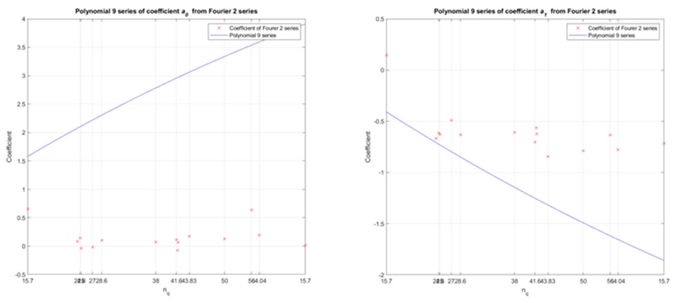
Through polynomial regression (with a polynomial of order 9) in the numerical model developed in MATLAB, the dependence between the values of coefficients a0, a1 (from the second-order Fourier function) and specific speed nq (11 pump–turbine models and 2 pump models) was determined for the Wh characteristic.
Figure 13.
Through polynomial regression (with a polynomial of order 9) in the numerical model developed in MATLAB, the dependence between the values of coefficients a0, a1 (from the second-order Fourier function) and specific speed nq (11 pump–turbine models and 2 pump models) was determined for the Wh characteristic.

Figure 14.
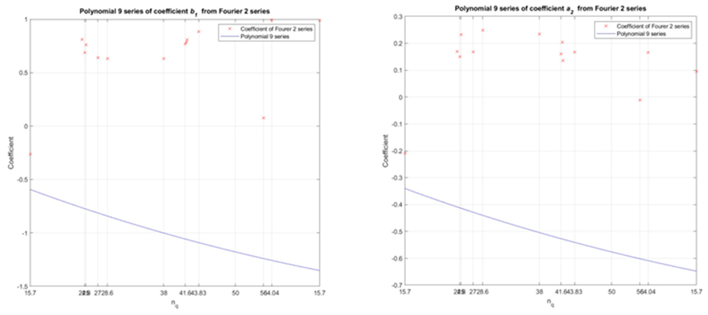
Through polynomial regression (with a polynomial of order 9) in the numerical model developed in MATLAB, the dependence between the values of coefficients b1, a2 (from the second-order Fourier function) and specific speed nq (11 pump–turbine models and 2 pump models) was determined for the Wh characteristic.
Figure 14.
Through polynomial regression (with a polynomial of order 9) in the numerical model developed in MATLAB, the dependence between the values of coefficients b1, a2 (from the second-order Fourier function) and specific speed nq (11 pump–turbine models and 2 pump models) was determined for the Wh characteristic.

Figure 15.
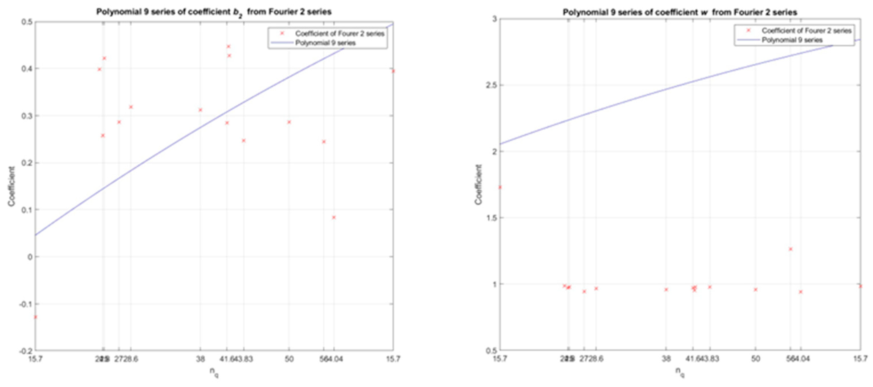
Through polynomial regression (with a polynomial of order 9) in the numerical model developed in MATLAB, the dependence between the values of coefficients b2, w (from the second-order Fourier function) and specific speed nq (11 pump–turbine models and 2 pump models) was determined for the Wh characteristic.
Figure 15.
Through polynomial regression (with a polynomial of order 9) in the numerical model developed in MATLAB, the dependence between the values of coefficients b2, w (from the second-order Fourier function) and specific speed nq (11 pump–turbine models and 2 pump models) was determined for the Wh characteristic.

Figure 16.
By polynomial regression (with a polynomial of order 9) in the numerical model developed in MATLAB, the dependence between the values of coefficients ao, a1 (from the second-order Fourier function) and specific speed nq (11 pump–turbine models and 2 pump models) was determined for the Wm characteristic.

Figure 17.
By polynomial regression (with a polynomial of order 9) in the numerical model developed in MATLAB, the dependence between the values of coefficients b1, a2 (from the second-order Fourier function) and specific speed nq (11 pump–turbine models and 2 pump models) was determined for the Wm characteristic.

Figure 18.
By polynomial regression (with a polynomial of order 9) in the numerical model developed in MATLAB, the dependence between the values of coefficients b2, w (from the second-order Fourier function) and specific speed nq (11 pump–turbine models and 2 pump models) was determined for the Wm characteristic.

Figure 19.
Comparison of Suter curves for the Wh characteristic obtained by re-calculating model curves Q11, n11, M11 with Suter curves obtained from universal equation, nq = 24.34 and 24.8.
Figure 19.
Comparison of Suter curves for the Wh characteristic obtained by re-calculating model curves Q11, n11, M11 with Suter curves obtained from universal equation, nq = 24.34 and 24.8.

Figure 20.
Comparison of Suter curves for the Wh characteristic obtained by re-calculating model curves Q11, n11, M11 with Suter curves obtained from universal equation, nq = 25 and 28.6.
Figure 20.
Comparison of Suter curves for the Wh characteristic obtained by re-calculating model curves Q11, n11, M11 with Suter curves obtained from universal equation, nq = 25 and 28.6.

Figure 21.
Comparison of Suter curves for the Wh characteristic obtained by re-calculating model curves Q11, n11, M11 with Suter curves obtained from universal equation, nq = 41.6 and 64.04.
Figure 21.
Comparison of Suter curves for the Wh characteristic obtained by re-calculating model curves Q11, n11, M11 with Suter curves obtained from universal equation, nq = 41.6 and 64.04.

Figure 22.
Comparison of Suter curves for the Wm characteristic obtained by re-calculating model curves Q11, n11, M11 with Suter curves obtained from the universal equation, nq = 24.34 and 24.8.
Figure 22.
Comparison of Suter curves for the Wm characteristic obtained by re-calculating model curves Q11, n11, M11 with Suter curves obtained from the universal equation, nq = 24.34 and 24.8.

Figure 23.
Comparison of Suter curves for the Wm characteristic obtained by re-calculating model curves Q11, n11, M11 with Suter curves obtained from universal equation, nq = 25 and 27.
Figure 23.
Comparison of Suter curves for the Wm characteristic obtained by re-calculating model curves Q11, n11, M11 with Suter curves obtained from universal equation, nq = 25 and 27.

Figure 24.
Comparison of Suter curves for the Wm characteristic obtained by re-calculating model curves Q11, n11, M11 with Suter curves obtained from the universal equation, nq = 28.6 and 64.04.
Figure 24.
Comparison of Suter curves for the Wm characteristic obtained by re-calculating model curves Q11, n11, M11 with Suter curves obtained from the universal equation, nq = 28.6 and 64.04.

Figure 25.
Schematic representation of components of pumping station.

Figure 26.
Change in head during transient processes at pump station (connection pump and pipe 1): comparison of obtained results for 13 specific speeds nq.
Figure 26.
Change in head during transient processes at pump station (connection pump and pipe 1): comparison of obtained results for 13 specific speeds nq.

Figure 27.
Change in discharge during transient process at pump station (connection pump and pipe 1): comparison of obtained results for 13 specific speeds nq.
Figure 27.
Change in discharge during transient process at pump station (connection pump and pipe 1): comparison of obtained results for 13 specific speeds nq.

Figure 28.
Change in dimensionless speed during transient processes at the pump: comparison of obtained results for 13 specific speeds nq.
Figure 28.
Change in dimensionless speed during transient processes at the pump: comparison of obtained results for 13 specific speeds nq.


Table 1.
Values of coefficients specified in the universal equation for the Wh characteristic.
| a0 (c1) | a0 (c2) | a0 (c3) | a0 (c4) |
| 0.00000000008265728147910180 | −0.000000029061457403003900 | 0.0000044563797292930600 | −0.0003908511288069320000 |
| a0 (c5) | a0 (c6) | a0 (c7) | a0 (c8) |
| 0.021587807156691600 | −0.7779210582576410 | 18.268604739268900 | −269.24654067798700 |
| a0 (c9) | a0 (c10) | a1 (c1) | a1 (c2) |
| 2256.073852668840 | −8170.186565443250 | −0.00000000003574826987209740 | 0.000000013284959440729400 |
| a1 (c3) | a1 (c4) | a1 (c5) | a1 (c6) |
| −0.0000021539386394449600 | 0.0001997420301777020000 | −0.011660699346564100 | 0.4438125887830780 |
| a1 (c7) | a1 (c8) | a1 (c9) | a1 (c10) |
| −10.995720789290900 | 170.69105909768900 | −1503.076337278080 | 5703.007866291280 |
| b1 (c1) | b1 (c2) | b1 (c3) | b1 (c4) |
| −0.00000000007545693999908280 | 0.000000025845257002692800 | −0.0000038551260024670600 | 0.0003284486762892260000 |
| b1 (c5) | b1 (c6) | b1 (c7) | b1 (c8) |
| −0.017601498848716700 | 0.6148165821380630 | −13.985903630865500 | 199.60428369467500 |
| b1 (c9) | b1 (c10) | a2 (c1) | a2 (c2) |
| −1619.808788457710 | 5686.005279970290 | 0.00000000004853501014984870 | −0.000000017313106387755800 |
| a2 (c3) | a2 (c4) | a2 (c5) | a2 (c6) |
| 0.0000026990431414927000 | −0.0002411556773051530000 | 0.013595507151620100 | −0.5009101639852780 |
| a2 (c7) | a2 (c8) | a2 (c9) | a2 (c10) |
| 12.042905981970900 | −181.84512743002200 | 1561.180298581870 | −5788.854265185760 |
| b2 (c1) | b2 (c2) | b2 (c3) | b2 (c4) |
| −0.00000000000127383719340139 | 0.000000000325499336592069 | −0.0000000269258577483385 | −0.0000000608514302740086 |
| b2 (c5) | b2 (c6) | b2 (c7) | b2 (c8) |
| 0.000160991178062167 | −0.0123557610666339 | 0.463796303315559 | −9.65109389182705 |
| b2 (c9) | b2 (c10) | w (c1) | w (c2) |
| 106.113132649951 | −478.811119088044 | 0.00000000007617383679759340 | −0.000000026492013127284700 |
| w (c3) | w (c4) | w (c5) | w (c6) |
| 0.0000040165086974174600 | −0.0003481612063995760000 | 0.019000243595516300 | −0.6763948591316100 |
| w (c7) | w (c8) | w (c9) | w (c10) |
| 15.691961350241300 | −228.50130238754600 | 1892.295034951600 | −6775.282084470940 |
Table 2.
Values of coefficients specified in universal equation for the Wm characteristic.
| a0 (c1) | a0 (c2) | a0 (c3) | a0 (c4) |
| 0.00000000007001706587787730 | −0.00000002501583155508980 | 0.000003904738113736460 | −0.0003491912666863700 |
| a0 (c5) | a0 (c6) | a0 (c7) | a0 (c8) |
| 0.01969645197701400 | −0.725829938836100 | 17.44890963741950 | −263.3977401451720 |
| a0 (c9) | a0 (c10) | a1 (c1) | a1 (c2) |
| 2260.388398637760 | −8377.01350286527 | −0.00000000000917920346698776 | 0.00000000390905486841779 |
| a1 (c3) | a1 (c4) | a1 (c5) | a1 (c6) |
| −0.000000712669136566865 | 0.0000731932114855007 | −0.00467292530266516 | 0.192408755177559 |
| a1 (c7) | a1 (c8) | a1 (c9) | a1 (c10) |
| −5.10821796821765 | 84.2463622056342 | −782.004920168192 | 3104.72992929313 |
| b1 (c1) | b1 (c2) | b1 (c3) | b1 (c4) |
| −0.00000000007140759190709090 | 0.00000002451861776936950 | −0.000003666867803655490 | 0.0003132713588738140 |
| b1 (c5) | b1 (c6) | b1 (c7) | b1 (c8) |
| −0.01683554373832690 | 0.589704417617438 | −13.44994606400680 | 192.3971195389380 |
| b1 (c9) | b1 (c10) | a2 (c1) | a2 (c2) |
| −1564.118084049990 | 5496.89652832734 | −0.00000000002473835428841850 | 0.00000000857389977038472 |
| a2 (c3) | a2 (c4) | a2 (c5) | a2 (c6) |
| −0.000001293799012428200 | 0.0001114657248249200 | −0.00603673362973466 | 0.212934147809491 |
| a2 (c7) | a2 (c8) | a2 (c9) | a2 (c10) |
| −4.88728990817866 | 70.3140700082219 | −574.701954526231 | 2029.92561253025 |
| b2 (c1) | b2 (c2) | b2 (c3) | b2 (c4) |
| 0.00000000001532603895634640 | −0.00000000534597810982802 | 0.000000813923958668984 | −0.0000709535832980723 |
| b2 (c5) | b2 (c6) | b2 (c7) | b2 (c8) |
| 0.00390090711682261 | −0.140186188779757 | 3.29082695837552 | −48.6175747114795 |
| b2 (c9) | b2 (c10) | w (c1) | w (c2) |
| 409.662879623748 | −1496.85732924952 | 0.00000000003725825084915130 | −0.00000001307237112503680 |
| w (c3) | w (c4) | w (c5) | w (c6) |
| 0.000002001304912505130 | −0.0001753365232788030 | 0.00967969358670688 | −0.348859201252643 |
| w (c7) | w (c8) | w (c9) | w (c10) |
| 8.19843384947085 | −120.9703220724220 | 1015.016628204550 | −3679.33688058800 |
Table 3.
Technical characteristics of components of pumping station.
| Pipe 1 Discharge (Q1) | Pipe 1 Wave Speed (a1) | Pipe 1 Friction Factor (f1) | Pipe 1 Diameter (D1p) |
| 0.5 m3/s | 900 m/s | 0.01 | 0.75 m |
| Pipe 1 Length (L1) | Pipe 2 Discharge (Q2) | Pipe 2 Wave speed (a2) | Pipe 2 Friction factor (f2) |
| 450 m | 0.5 m3/s | 1100 m/s | 0.012 |
| Pipe 2 Diameter (D2 p) | Pipe 2 Length (L2) | Pump efficiency (η) | Pump moment of inertia (WR2) |
| 0.75 m | 550 m | 0.84 | 16.85 kg·m2 |
| Pump rated speed of rotation (n*) | Pump rated head (H*) | Pump rated discharge (Q*) | |
| 1100 rpm | 60 m | 0.25 m3/s |
Disclaimer/Publisher’s Note: The statements, opinions and data contained in all publications are solely those of the individual author(s) and contributor(s) and not of MDPI and/or the editor(s). MDPI and/or the editor(s) disclaim responsibility for any injury to people or property resulting from any ideas, methods, instructions or products referred to in the content. |
© 2023 by the authors. Licensee MDPI, Basel, Switzerland. This article is an open access article distributed under the terms and conditions of the Creative Commons Attribution (CC BY) license (https://creativecommons.org/licenses/by/4.0/).
Share and Cite
MDPI and ACS Style
Giljen, Z.; Nedeljković, M. Universal Form of Radial Hydraulic Machinery Four-Quadrant Equations for Calculation of Transient Processes. Energies 2023, 16, 7736. https://0-doi-org.brum.beds.ac.uk/10.3390/en16237736
AMA Style
Giljen Z, Nedeljković M. Universal Form of Radial Hydraulic Machinery Four-Quadrant Equations for Calculation of Transient Processes. Energies. 2023; 16(23):7736. https://0-doi-org.brum.beds.ac.uk/10.3390/en16237736
Chicago/Turabian StyleGiljen, Zdravko, and Miloš Nedeljković. 2023. "Universal Form of Radial Hydraulic Machinery Four-Quadrant Equations for Calculation of Transient Processes" Energies 16, no. 23: 7736. https://0-doi-org.brum.beds.ac.uk/10.3390/en16237736
Note that from the first issue of 2016, this journal uses article numbers instead of page numbers. See further details here.