Article

Investigation of the Partial Shading Effect of Photovoltaic Panels and Optimization of Their Performance Based on High-Efficiency FLC Algorithm

1
Department of Mechanical Engineering, Faculty of Mechanical Engineering and Mechatronics, Polytechnic University of Bucharest, Independence Street no. 13, District 6, 060042 Bucharest, Romania
2
Department of Applied Physics, Faculty of Applied Sciences, Polytechnic University of Bucharest, Independence Street no. 13, District 6, 060042 Bucharest, Romania
3
Academy of Romanian Scientists (AOSR), Ilfov Street 3, 030167 Bucharest, Romania
*
Author to whom correspondence should be addressed.
Submission received: 20 November 2022 / Revised: 10 January 2023 / Accepted: 16 January 2023 / Published: 20 January 2023
(This article belongs to the Special Issue Analysis and Numerical Modeling in Solar Photovoltaic Systems)

Abstract

:
The present work proposes an enhanced method of investigation and optimization photovoltaic (PV) modules by approaching and using MPPT (Maximum Power Point Tracking) technique to improve their output power. The performance of the PV panels is strongly influenced by the operating conditions, especially regarding the solar irradiance, temperature, configuration, and the shading (due to a passing cloud or neighboring buildings); all these cause, both on energy conversion loss, and further on non-linearity of the I-V characteristics. From this reason, the present study could have a high relevance based on the improvement of the performances (including the efficiency) of the shaded photovoltaic panels and would quantify the impact of a complex approach represented by numerical modeling and experimental validation. For a better understanding of these issues determined by partial shading, and improvement of MPP tracking, it is required to study the behavior of individual panels. For the best accuracy of the implemented models a comparative analysis and optimized method of the PV modules was considered based on: (1) the influence of temperature and solar irradiance and behavior of the PV modules in partial shading conditions; (2) a comparison between the optimized output power of four algorithms (FLC—Fuzzy Logic Controller, P&O—Perturb and Observe, IncCond—Incremental Conductance and RC Ripple Correlation) and the selection of the best one (FLC); (3) discussion of customized/improved fuzzy logic controller (FLC) algorithm on five operation points introduced in order to increase PV module efficiency under fluctuating weather conditions and rapidly changing uncertainties. Furthermore, the FLC provides a set of rules useful for predicting the current-voltage behavior and the maximum power points of shaded photovoltaic modules. This FLC algorithm was implemented in a specialized software, namely MATLAB/Simulink. The authors highlighted the development and implementation of a numerical simulation model for an advanced PV module to determine its behavior under different operating conditions and improve its performance. The essence of the authors’ research and the motivation of this work is described. The authors were able to stabilize and improve the output performance of the PV module. The results concerning the shading effect as well as the shading patterns were developed, demonstrated, and experimentally validated. These results could be applied for the actual photovoltaic installations, respectively complex stand-alone or grid-connected photovoltaic systems.

1. Introduction

Due to various incentive programs and local market conditions in several European countries, as well as around the world, the photovoltaic (PV) systems represent a widespread solution for residential houses and other autonomous applications [1,2,3]. This approach raises new and important issues related to the efficiency, reliability, and safety of the PV systems, either autonomous or connected to the electrical grid [4].
The photovoltaic systems have increasing roles in modern electric power energy mix due to the continuing decline in the world’s conventional energy sources. The major advantages associated with photovoltaic systems are: (1) no moving parts; (2) noise is not produced; (3) little or no maintenance requirement and non-polluting; (4) they are renewable; (5) they are highly modular and highly reliable; (6) they can be installed almost anywhere [5].
The quality aspects of the electricity production, namely its reliability and stability influence high demand for electricity supply in terms of an increasing consumer safety [6]. However, the electricity production based on renewables raises the problems of compatibility with the electricity grid. A significant issue of the photovoltaic (PV) system is the power storage and represents an important aspect for performance improvement in solar power building communities [7,8,9,10]. The existing studies have developed various design methods for distributed batteries and shared batteries; however, the existing design methods are based on community aggregated energy mismatch, which may avoid battery oversizing, but would determine another severe problem, respectively, an excessive electricity loss in the sharing process due to the long-distance power transmission [11,12,13,14].
Storage is the key for a future-proofing energy; this issue could be solved using solar energy generation that is intermittent [15,16,17,18]. An important perspective and challenge in future research could be considered the energy storage in terms of security and high efficiency.
One of the literature gaps in the analyze of different algorithms applications connected with the operational optimization of PV systems regarding their performances, stability and durability based on partial shading conditions was discussed in the present study dedicated to the MPPT-FLC [19,20,21,22,23,24]. The obtained results could be considered for other algorithms utilization regarding the optimization of autonomous or grid connected various PV systems [25].
In order to achieve high performance and competitiveness of PV systems, it is necessary to achieve individual analyses on each type of PV system or application, respectively, on each type of application in which they can be integrated. The operational optimization of PV systems is possible by optimization of MPPT-FLC algorithm that led to the improvement of the electrical performance of PV systems in fluctuating operating conditions (random meteorological parameters) [26,27,28,29].
The authors aimed to Increase the performance of PV generator by adopting an advanced FLC algorithm that was implemented in the MATLAB/Simulink environment. On this basis, it is possible to increase the output power of PV systems, as well as its optimization from the point of view of the electricity consumer.
The valuable contribution of this paper was related with the implemented optimization of a PV generator by: (1) development and implementation of a upper approach based on series-parallel investigation in order to study the shading effects for the analyzed PV generator; (2) optimized operation of a PV generator by numerical modelling for the study of the influence of temperature and solar irradiance on PV device performances, as well as its behavior for partial shading condition; (3) comparative analysis of four types of MPPT algorithms in order to choose and implement the most efficient one in the operational optimization of the PV generator; and (4) significant increasing of the output power of PV generator based on a novel and advanced FLC algorithm to be developed for investigation of the PV generator with five operating points.
The organization of this study was based on an improved numerical simulation model; it was implemented in MATLAB Simulink, with direct implication in increasing the performance of PV generator. In this way, it is possible to respond efficiently to the varying character of the output parameters of the PV generator; interesting results would be obtained regarding the behavior and evolution of electrical parameters of the PV generator in different conditions.
The major objective of the present article was to develop a unifying approach of the methods and models used for investigation of PV generator; in this way, it would be possible to determine the influence of temperature and shading effects on performance of PV generator.
Another objective—the covered—gap is the accuracy and complexity of the research work that covers a wide spectrum in terms of the flow of information and obtained results, taking into account the existence of the insufficient practice in the specialized literature.

2. Knowledge and State of the Art

According to experts, the owners of these PV systems could lose up to 30% of the potential production of their photovoltaic installation due to shading, and this situation does not occur because the entire panel is shaded. It is enough for 20% of the surface of the solar panel to be shaded, a fact for which its output power leads to a decrease in electrical efficiency by up to 50%, according to some reports and research studies in the field. Mainly, this is due to the way the solar cells in an array are connected in the system [30,31,32,33,34].
The shading effect occurs when a photovoltaic system does not receive the same level of incident solar irradiance throughout the system due to some obstructions. Under these conditions, cells that receive a lower level of solar irradiance can absorb power instead of producing it. For this reason, bypass diodes are used to reduce the impact of the shading effect and to protect the solar panels [35,36,37,38]. Photovoltaic array models are configured with two or one diode. Bypass diodes are generally used every 10 cells in the panel (depending on the number of cells that make up the panel). Based on the configuration of the photovoltaic array, the shading effect on the specific PV system can be studied. An efficient and unifying approach to investigating and determining the behavior of PV modules, a maximum power point tracking system can be used together with a specific algorithm such as fuzzy logic, disturbance and observation, buck converter, incremental inductance, i.e., [39,40,41,42,43,44].
Conventional arrays of solar cells are connected in PV panels in a series of parallel “strings”. If an array is affected by shadowing, then the losses are passed on to the rest of the cell chain. To prevent complete failure of all cells, the installation usually includes bypass diodes [45]. These then redirect the current, bypassing the damaged/inefficient cells. However, even though the array does not fail together—in the same way that an electrical device for lighting that continues a series of lighting mixtures goes out when one fails—still, in the photovoltaic panel, the energy is restricted from the cells and thus lowers the voltage of the entire string, which implicitly causes a decrease in the energy efficiency of the photovoltaic device [46,47,48].
A shaded module in a string can significantly reduce its output power, however, a shaded module in a string does not reduce the output power of a parallel string. Therefore, a feasible and efficient solution is given by the grouping of shaded modules in separate strings (parallel series), thus, the total output power of the photovoltaic array can be maximized [49,50,51]. For example, in a real PV system, it can be beneficial to group modules that receive shade from parapets in strings and keep modules that do not receive shade from parapets in separate, parallel strings. In this way, the unshaded strings can maintain a higher current and power. However, to determine the effect in which shading affects the PV module, a theoretically complex approach based on modelling and numerical simulation of the electrical characteristics of the PV array is required [52].
Another method to improve the efficiency of a PV module in the case of partial shade is the implementation of a DC optimizer whose role is to adjust the output voltage and current and implicitly to maintain the maximum power without compromising the performance of other modules. This is achievable and possible by studying algorithms for optimizing the maximum power point, such as the FLC (Fuzzy Logic Controller) technique [53]. Such an approach allows for modelling and simulation the behavior of PV modules in an efficient manner that also allows the adjustment of the way the panels work, respectively, their operational optimization. At the same time, an optimization method based on MPP tracking algorithms ensures accuracy in terms of output power optimization, which is why numerous studies and researchers have continued to develop these models in order to increase the degree of usefulness and performance in terms of efficiency PV systems [54].
A concrete example, when a shaded module produces electricity but with a lower current, the DC optimizer (based on one of the established MPP tracking algorithms) will increase the output current to match the current flowing through the unshaded modules; to compensate, the optimizer reduces its output voltage by the same amount as it increases the current. This allows the shaded module to produce the same amount of electricity without blocking the output of other modules [55]. In order to understand the shading influence, in Figure 1 is schematically represented the effect in the case of photovoltaic cells and the implications regarding the output power, and also where we can apply the optimization.
In the specialized literature, the subjects regarding the partial shading and optimization of PV systems based on MPPT techniques are of great interest and were discussed by several researchers in the field, among which we could mention: (1) Chayut Tubniyom et. al., studied the effect of partial shading patterns and degrees of shading on Total Cross-Tied (TCT) photovoltaic array configuration; they proved the shading effect on PV modules through numerical simulation. Three standard configurations of PV array consist of series-parallel (SP) [56]; (2) Guoqian Lin and al. studied in their work entitled “Photovoltaic Modules Selection from Shading Effects on Different Materials”, a series of efficiency improvement methods for production and reduction of investment costs in the photovoltaic system using the symmetry concept, combining both mathematical and engineering principles for solar energy. The study builds a symmetrical photovoltaic model and uses series-parallel circuit theory, piecewise function, and MATLAB simulation [57]; (3) Alonso Gutiérrez Galeano et al, studied a simplified approach for modelling and analyzing the performance of partially shaded photovoltaic modules performance using the shading ratio. This approach integrates features of shadow area and shadow opacity into the PV cell model. The studied methodology aims to improve the description of shaded photovoltaic systems by specifying an experimental procedure for quantifying the shade impact. In addition, with the help of image processing, shading ratio analysis provides a set of useful rules for predicting the current-voltage behavior and peak power points of shaded PV modules. This correlation of shading ratio and shading patterns can contribute to the supervision of real photovoltaic installations [58]; (4) Carlos Robles Algarín et al., in their work entitled “Fuzzy Logic Based MPPT Controller for a PV System” discussed the need to implement maximum power point tracking (MPPT) controllers in order to obtain a maximized power for photovoltaic systems, regardless of variations in climatic conditions. It proposes a fuzzy controller and demonstrates that the results of simulation and numerical modelling show the scientific superiority and accuracy regarding the developed model [59]; (5) Qiang Zhao et al., in their paper entitled “A New PV Array Fault Diagnosis Method Using Fuzzy C-Mean Clustering and Fuzzy Membership Algorithm”, studied the PV array’s electrical characteristics’ behavior under fault conditions, and a novel PV array fault diagnosis method was proposed based on Fuzzy C-Mean (FCM) and fuzzy membership algorithms [60]; and (6) Simoes Marcelo Godoy et al. described in their paper the analysis, modelling, and implementation of a fuzzy based photovoltaic peak power tracking system. An analytical model was built for the PV system on the basis of the manufacturer characteristics. The solar panel was integrated with the converter model and a fuzzy algorithm was developed in order to perform an on-line search procedure to track the maximum power continuously [61].

3. Advanced Models of the PV Generator

3.1. PV Solar Cell Advanced Model

The mathematical model for two diodes model can be used for description of the electrical behavior of a solar cell. Different advanced models would be considered in the case of a PV cell operating under partial shading conditions [62,63]. One of these models is the Bishop Model [63], which requires and imposes a negative voltage on its terminals (negative cell voltage and positive cell current, thus consuming power). Another model is the Direct Reverse Model [64] that would reproduce the operation of a solar cell in either direct or reverse biasing modes for the influence of temperature and solar irradiance variations. Analyzed are the following: (1) positive cell voltage and current and (2) negative cell voltage and positive cell current, needed for power analysis and losses estimation during partial shading conditions. Future work could apply optimization techniques to solve the parameter estimation problem, which may reduce both estimation errors and computation time.
Therefore, a standard solar cell model is used. The current Icell provided by the cell is given by Figure 2:
I c e l l = I p h I r I s h
where Iph, Ir and Ish are the photo-generated current, the reverse current, and the shunt current, respectively.
It is denoted the voltage across the cell by Vcell. Then, the voltage V over the shunt resistance Rsh is given by V = Vcell + RsIcell. Here, Rs is the solar cell series resistance. The shunt current is given by Ish = V/Rsh. The reverse current is given by:
I r = I 0   exp q V B c e l l K T c e l l 1
where I0, Bcell, K and Tcell are the reverse saturation current, solar cell thermal voltage constant, Boltzmann’s constant, and the cell temperature, respectively. Additionally, q is the electron’s electric charge. The above relationships allow the writing of Equation (2) as:
I c e l l = I p h I 0 exp exp q V c e l l + R s I c e l l B c e l l K T c e l l 1 V c e l l + R s I c e l l R s h  
The following relations can be used for silicon solar cells:
I p h = G T · τ α · s A c e l l  
I 0 = K c e l l A c e l l T c e l l 3 exp E g K T c e l l
where GT, τ α , s and Acell are: the solar global irradiance at the level of the solar cell, the effective transmittance–absorbance product of the cell, a constant and the surface area of a solar cell, respectively [65]. Additionally, Kcell and Eg are the cell constant and the cell material’s band gap, respectively [66].

3.2. PV Solar Module Advanced Model

Several solar cell interconnection schemes were studied in [67] from the viewpoint of the cell reliability (the ability to continue operation without failure throughout a certain time). These schemes were: (a) a simple series-parallel module consisting of M parallel strings with each string having N solar cells connected in series; (b) a total cross tied system obtained from the simple series-parallel module by connecting ties across each row of junctions; and (c) a bridge linked system, consisting of solar cells interconnected in a bridge rectifier fashion.
The method proposed in this article is developed for a simple series-parallel scheme. It can also be implemented for other interconnection schemes. A PV module of M parallel strings, each of them consisting of N identical solar cells, is shown in Figure 3. The relation between the voltage across the PV module, Vmodule, and that across the solar cell, Vcell, is given by:
I c e l l = V m o d u l e + I m o d u l e R s , m o d u l e N
where Rs,module is the PV module series resistance. The current I’ through the PV module shunt resistance Rs,shunt is given by:
I = V m o d u l e + I m o d u l e R s , m o d u l e R s , m o d u l e
and the current I” is given by:
I = I c e l l M = I m o d u l e + I
Using the solar cell Equation (3) and Equations (6)–(8) yields, after some algebra, the PV module Imodule–Vmodule characteristics (see also [68,69]):
R s h ,   m o d u l e   N R s h + N R s + M R s , m o d u l e + N R s , m o d u l e R s h + R s N R s h N R s h , m o d u l e   I m o d u l e = M I p h N R s h + N R s + M R s , m o d u l e N R s h N R s h , m o d u l e   V m o d u l e M I 0 exp q M + N R s R s h , m o d u l e + V m o d u l e + N R s + M R s , m o d u l e + N R s R s , m o d u l e R s h , m o d u l e I m o d u l e N M B c e l l k T c e l l 1
The electric power Pmodule provided by the PV module is given by
P m o d u l e = I m o d u l e   V m o d u l e  
The energy balance at the level of the whole PV module is given by:
M N A c e l l s G T τ α M N A c e l l U c e l l   T c e l l T a I m o d u l e V m o d u l e = 0
where Ucell and Tcell are average PV module values of the convection heat loss coefficient and cell temperature, respectively, while Ta is the environment temperature. The first term in Equation (11) gives the rate of solar energy absorbed by the PV module, while the second term is the heat flux transferred by convection from the solar cells to the ambient environment. The third term represents the electric energy leaving the PV module. The PV module efficiency, η is defined as the ratio between the electrical output power and the incident solar radiation power, i.e.,
η = P m o d u l e G T A m o d u l e
where the PV module area is given by Amodule = MNAcell.
Specific interesting points linked with the I-V curve, respectively: the short-circuit point, the open-circuit point and the maximum power point are obtained and discussed in the following chapters based on numerical modelling in MATLAB/Simulink software.

4. Numerical Modelling of the Electrical Characteristics of the PV Module: Influence of Temperature and Solar Irradiance

4.1. Basics

PV modules are given a power rating at standard test conditions of 1000 W/m2 with an AM (air mass) of 1.5 at a module temperature of 25 °C, but these conditions do not represent what is typically experienced under outdoor operation. The results have confirmed that the output of PV modules changes seasonally in proportion to changes in solar radiation. This provided strong evidence that the variation in solar radiation should be taken into account for an optimum design. The method proposed in this paper is used to study the influence of various climates on the optimal PV cells interconnections.
The drawing of a PV module was entirely developed in MATLAB/Simulink to characterize the electrical characteristics (see Figure 4). It presents the methodology of the simulation technique used for electrical characteristics of the PV module, namely, the I-V and P-V characteristics of the PV module. A notable advantage of this approach in the MATLAB environment is the fact that once created, the photovoltaic generator model it can be later interfaced with current system models that make possible to simulate complex photovoltaic systems and their interaction with other systems. A major advantage of using MATLAB software is its availability in most academic research and industrial organizations, being useful for a wide range of engineering disciplines.

4.2. The Study of the Temperature Influence on the PV Module Electrical Characteristics

In this chapter, the modeling and simulation of the solar cell and PV panel(module) allowed to obtain its behavior for different values of temperature and solar irradiance, respectively. The current-voltage (I-V) characteristics of the PV generator were determined for 1000 W/m2 at different values of temperature and solar irradiance in relation to the reference size (STC). In the case of the power-voltage characteristics of the PV generator, both the values of solar irradiance and temperature were varied. The characteristics of the PV generator are presented in Table 1.
It is worth highlighting the way in which these main electrical parameters behave at temperature variations, namely: (a) short-circuit current Isc (Figure 5; (b) open-circuit voltage Voc (Figure 6); (c) maximum power Pmax (Figure 7); and (d) the fill factor FF (Figure 8). This was made possible by activating a function in the model that allows the random generation of temperature to simulate the real operating conditions of the PV generator. The graphical representation of the main parameters of the PV generator considered the real operating conditions, where the temperature was observed in the range of 20–60 °C (this temperature was recorded in Romania, in Constantza city, in August 2022). PV modules are given a power rating at 1000 W/m2 with an AM (airmass) of 1.5.
In the same way, the output characteristics of the PV module were determined in relation to the variation of the solar irradiance, within the limits indicated in the obtained figures; we can extract from the diagram the values of the maximum power points associated with the maximum values of current and voltage (Imp and Vmp), as seen in Figure 5c). For the tested module (by simulation) a maximum power was obtained of approximately 500 W, a value comparable to that of existing PV modules on the market (real). The final analysis of the PV generator is presented from the point of view of the main electrical parameters (indicators): Isc, Voc, Pmax, FF.
The results show that all electrical parameters of the PV module, such as maximum output power, open circuit voltage, short circuit current, and fill factor, have changed with temperature variation. PV module performance decreases with increasing temperature, fundamentally owing to increased internal carrier recombination rates caused by increased carrier concentrations. The operating temperature plays a key role in the photovoltaic conversion process. Both the electrical efficiency and the power output of a photovoltaic (PV) module depend linearly upon the operating temperature.

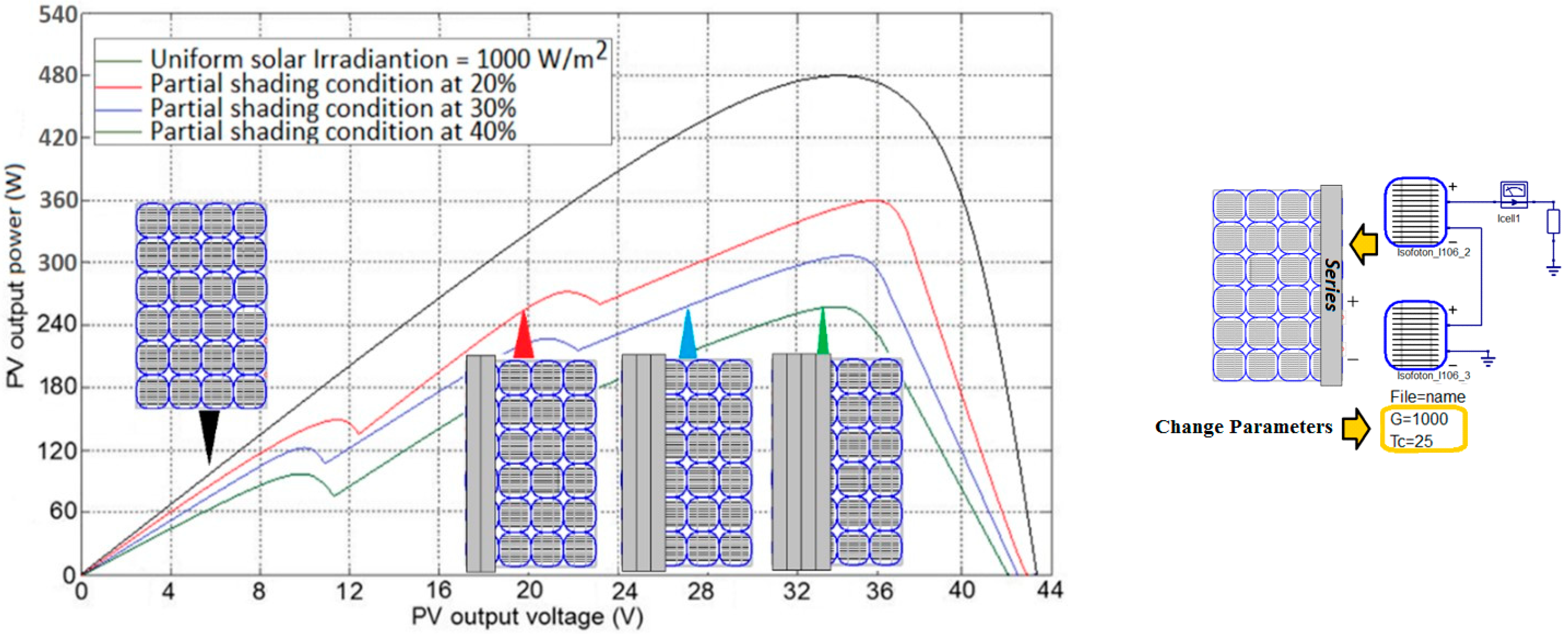
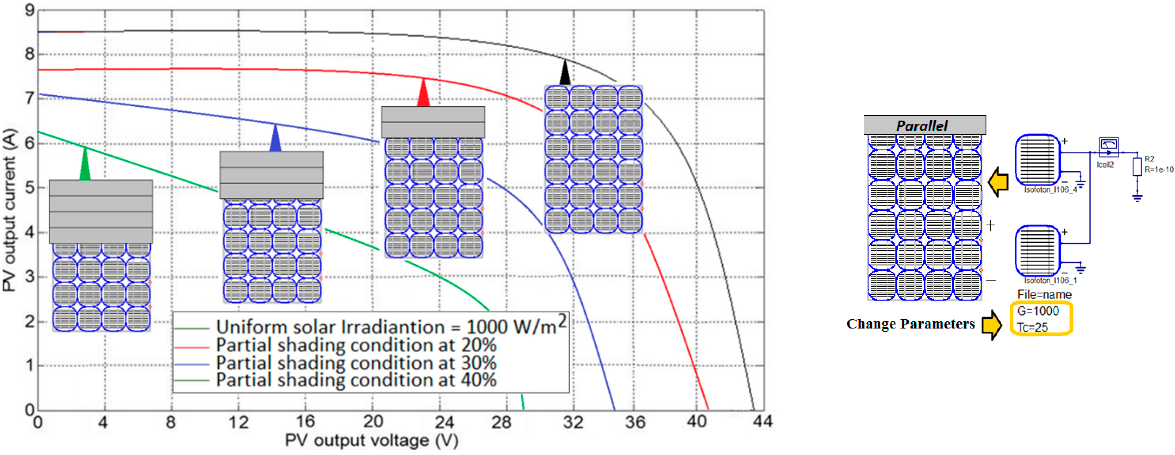
4.3. The Study of Behaviour and Response of the PV Module to STC Irradiance & Partial Shading Conditions

To analyze the dynamic behavior of the studied PV module, an algorithm based on the series-parallel method was introduced; the considered model described in Section 3 was implemented and evaluated in MATLAB/Simulink environment, considering the changes of solar irradiance and temperature registered by the photovoltaic system, in conditions of its partial shading. Three situations of partial shading of the PV module were investigated: 20%, 30% and 40%. Under conditions of complete (standard) solar irradiance, characteristics I-V have a single maximum power point; on the other hand, when the PV module is partially shaded, there are several maximum power points.
The I-V and P-V characteristics curves of the PV module, for different shading conditions and types of shading (series and parallel), are represented in Figure 9, Figure 10, Figure 11 and Figure 12; they indicate that the PV module depends very much on the applied solar irradiance, and the fluctuating character, as well as the environmental factors do not allow the equal distribution of the partial shading on the photovoltaic module, as a result, the application of optimization algorithms (in our case MPPT-FLC) makes it possible to gain power, even if it is not uniform.
The simulation results for the three shading situations suggest that the partially shaded mode does not cause a significant reduction in output power, even if the shadow value reaches 40%, with a gap due to the MPPT-FLC optimization algorithm.

5. The Performance Evaluation of the PV Generator Based on MPPT—FLC: Case Study

5.1. The Theoretical Aspects of Fuzzy Logic Algorithm

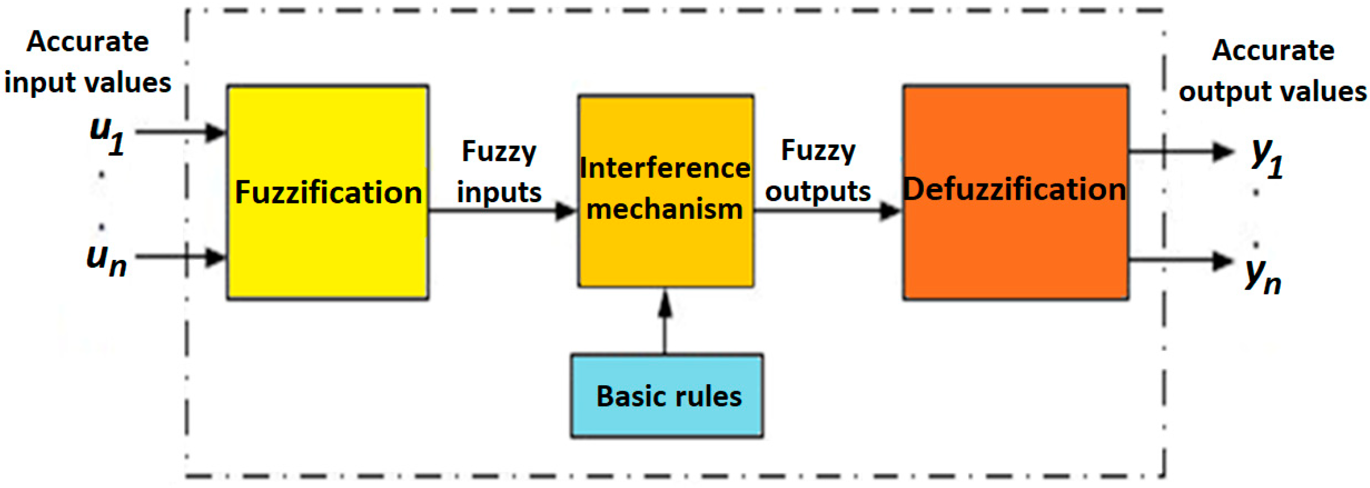
5.1.1. Fuzzy Block Diagram

The mathematical model underlying fuzzy logic is presented below, considering the most accurate definition of the terminology that characterizes this method, namely: variables, values and rules in fuzzy language [70,71,72,73]. After choosing the FLC inputs and outputs, there must be a language description for each of the respective input and output sizes.
Taking into account the complexity of Fuzzy Logic Algorithm given by: (1) membership function; (2) input and output variables; (3) fuzzification mechanism, interference mechanism (rules) and defuzzification mechanism, a list of abbreviations was created in order to define the terminology of the FLC.
For a fuzzy system, we will describe: (1) the fuzzy input as ui and its variable as u i ^ , (2) for the fuzzy output, we will have yi and the output size variable will be described as y i ^ . After establishing the input and output of the FLC, a description of each variable must be made, namely, u i ^ and y i ^ . In Figure 13 is presented the fuzzy block diagram that converts the input values to fuzzy values, and then through the interference mechanism, the FLC outputs could be obtained.
The mathematical characterization of the triangular member entry function, where μ , the membership function, is shown below:
μ s m a l l u = 1                                                               i f   u   0                                   max 0.1 u 0.5         o t h e r w i s e              
μ s m a l l u = 1                                                               i f   u   0.25                                   max 0.1 u 0.25         o t h e r w i s e              
μ m e d i u m u = max 0.1 + u 0.5 0.5   i f   u   0.5   max 0.1 + 0.5 u 0.5   o t h e r w i s e    
μ h i g h u = max 0.1 + u 0.75 0.75   i f   u   0.75   1   o t h e r w i s e    
μ h i g h u = max 0.1 + u 0.5 0.5   i f   u   1   1   o t h e r w i s e    
The output variable is represented by a normalized fuzzy set of five triangular MFs: Large Negative (NB), Medium Negative (NM), Low Negative (NS), Zero (ZO), Small Positive (PS), Medium Positive (PM) and Large Positive (PB) (see Figure 14). The mathematical characterization of the membership for the triangular function is presented below in the relations (18–24).
μ N B Δ C = 1   i f   Δ C   1   max 0.1 + 1 Δ C 0.5   o t h e r w i s e  
μ N M Δ C = 1   i f   Δ C   0.75   max 0.1 + 1 Δ C 0.75   o t h e r w i s e  
μ N S Δ C = max 0.1 + Δ C + 0.5 0.5   i f   Δ C   0.5   max 0.1 + 0.5 + Δ C 0.5   o t h e r w i s e    
μ Z O Δ C = max 0.1 + Δ C 0.5   i f   Δ C   0   max 0.1 + Δ C 0.5   o t h e r w i s e  
μ P S Δ C = max 0.1 + Δ C 0.5 0.5   i f   Δ C   0.5   max 0.1 + 0.5 Δ C 0.5   o t h e r w i s e    
μ P M Δ C = max 0.1 + Δ C 0.75 0.5   i f   Δ C   0.75   max 0.1 + 0.75 Δ C 0.5   o t h e r w i s e    
μ P B Δ C = max 0.1 + Δ C 1 0.5   i f   Δ C   1   1   o t h e r w i s e  
The P-V characteristics of the PV panel could be divided in five regions (with 5 points power operations), depending on the value of the absolute power slope—Sa (see Figure 15). The FLC controller will cause the change to a new step; ΔC—exit membership is based on the old disturbance—Cold to reach the MPP.

5.1.2. Interference Mechanisms

The two interference mechanisms are fuzzification and defuzzification. They will be discussed in the following:
(A)
Fuzzification:
Assuming that the operating point is at P1, and the absolute value of the slope Sa is high, it is remarked that the operating point is far from MPP. The old disturbance (Cold) can have three different values: (a) if Cold is small, then the change in the step size ΔC must be large positive (PB) to reach MPP quickly; (b) if Cold is medium, the change in the step size ΔC must be small’ positive (PM) to reach the MPP without oscillating around it; (c) if Cold is large, the change in step size ΔC must be small positive (PS) to avoid overtaking the MPP in the opposite direction, leading to oscillations.
  • Operating point: P1
    -
    If Sa is high and Cold is small, then ΔC is positively high
    μ premise   1 = min μ high S a , μ small   C old
    μ 1 Δ C = min   μ PB Δ C , μ premisa   1  
    -
    If Sa is high and Cold is medium, then ΔC is positive small
    μ p r e m i s e   2 = min μ h i g h S a , μ m e d i u m   C o l d
    μ 2 Δ C = min   μ P M Δ C , μ p r e m i s e   2
    -
    If Sa is high and Cold is high, then ΔC is zero
    μ p r e m i s e   3 = min μ h i g h S a , μ h i g h   C o l d
    μ 3 Δ C = min   μ P S Δ C , μ p r e m i s e   3
Assuming that the operating point is at P2, where the absolute value of the slope Sa is average, it means that the operating point is closer to the MPP than in the previous case, but still does not give it up. The Cold can also have three different values in this case. (a) If Cold is small, then the change in step size ΔC must be small’ positive (PM) to reach the MPP without oscillating around it; (b) if Cold is medium, the change in step size ΔC must be small positive (PS) to avoid overtaking the MPP in the opposite direction leading to oscillations; (c) if Cold is large, the change in step size ΔC must be zero (ZO), so as to not exceed MPP.
  • Operating point: P2
    -
    If Sa is high and Cold is small, then ΔC is positively high
    μ p r e m i s e   4 = min μ h i g h S a , μ s m a l l   C o l d
    μ 4 Δ C = min   μ P M Δ C , μ p r e m i s a   1  
    -
    If Sa is high and Cold is medium, then ΔC is positive small
    μ p r e m i s e   5 = min μ h i g h S a , μ m e d i u m   C o l d
    μ 5 Δ C = min   μ P S Δ C , μ p r e m i s e   2
    -
    If Sa is high and Cold is high, then ΔC is zero
    μ p r e m i s e   6 = min μ h i g h S a , μ h i g h   C o l d
    μ 6 Δ C = min   μ Z O Δ C , μ p r e m i s e   3
Assuming that the operating point is at P3, where the absolute value of the slope Sa is average, it means that the operating point is closer to the MPP than in the previous case, but still does not give it up. The Cold can also have three different values in this case. (a) If Cold is small, then the change in step size ΔC must be small positive (PS) to reach the MPP without oscillating around it; (b) if Cold is medium, the change in step size ΔC must be zero (ZO) to avoid overtaking the MPP in the opposite direction leading to oscillations; (c) if Cold is large, the change in step size ΔC must be negatively small (NS), so as to not exceed MPP.
  • Operating point: P3
    -
    If Sa is medium and Cold is small, then ΔC is positive small
    μ p r e m i s e   7 = min μ m e d i u m S a , μ s m a l l   C o l d
    μ 7 Δ C = min   μ P S Δ C , μ p r e m i s e   4
    -
    If Sa is medium and Cold is medium, then ΔC is zero
    μ p r e m i s e   8 = min μ m e d i u m S a , μ m e d i u m   C o l d
    μ 8 Δ C = min   μ Z O Δ C , μ p r e m i s e   5
    -
    If Sa is medium and Cold is high, then ΔC is negative small
    μ p r e m i s e   9 = min μ m e d i u m S a , μ h i g h   C o l d
    μ 9 Δ C = min   μ N S Δ C , μ p r e m i s e   6
Assuming that the operating point is at P4, where the absolute value of the slope Sa is average, it means that the operating point is closer to the MPP than in the previous case, but still does not give it up. The Cold can also have three different values in this case. (a) If Cold is small, then the change in step size ΔC must be zero (ZO) to reach the MPP without oscillating around it; (b) if Cold is medium, the change in step size ΔC must be negative small (NS) to avoid overtaking the MPP in the opposite direction leading to oscillations; (c) if Cold is large, the change in step size ΔC must be negatively small’ (NM), so as to not exceed MPP.
  • Operating point: P4.
    -
    If Sa is medium and Cold is small, then ΔC is positive small
    μ p r e m i s e   10 = min μ m e d i u m S a , μ s m a l l   C o l d
    μ 10 Δ C = min   μ Z O Δ C , μ p r e m i s e   7
    -
    If Sa is medium and Cold is medium, then ΔC is zero
    μ p r e m i s e   11 = min μ m e d i u m S a , μ m e d i u m   C o l d
    μ 11 Δ C = min   μ N S Δ C , μ p r e m i s e   8
    -
    If Sa is medium and Cold is high, then ΔC is negative small
    μ p r e m i s e   12 = min μ m e d i u m S a , μ h i g h   C o l d
    μ 12 Δ C = min   μ N M Δ C , μ p r e m i s e   9
Assuming that the operating point is at P5, where the absolute value of the slope Sa is small, then it means that the operating point is close to the MPP. The old step can have three different values in this case. (a) If Cold is small, then the change in step size ΔC must be negative small (NS) to avoid overtaking the MPP in the opposite direction leading to oscillations. (b) If Cold is medium, the change in step size ΔC must be negative small’ (NM), so as to not exceed MPP; (c) if Cold is large, the change in step size ΔC must be large negative (NB) so as to not exceed MPP.
  • Operating point: P5
    -
    If Sa is small and Cold is small, then ΔC is zero
    μ p r e m i s e   13 = min μ s m a l l S a , μ s m a l l   C o l d
    μ 13 Δ C = min   μ N S Δ C , μ p r e m i s e   10
    -
    If Sa is small and Cold is medium, then ΔC is negative small
    μ p r e m i s e   14 = min μ s m a l l c S a , μ m e d i u m   C o l d
    μ 14 Δ C = min   μ N M Δ C , μ p r e m i s e   11
    -
    If Sa is small and Cold is high, then ΔC is negative high
    μ p r e m i s e   15 = min μ m i c S a , μ h i g h   C o l d
    μ 15 Δ C = min   μ N B Δ C , μ p r e m i s e   12
Based on these results, Sa determines three rules for the operating points P1, P2, P3, P4 and P5 (see Figure 15). The FLC rules are presented in Table 2. The interference operator compares the rules for each of the MF inputs and chooses the minimum rule.
(B)
Defuzzification:
The second stage in the FLC process is defuzzification, which takes the input fuzzy values and generates real numbers.
Δ C r e a l =   1 u 15   Δ C + 0.75 u 14   Δ C + 0.5 u 13   Δ C i = 1 15 u i   Δ C + 0.75 u 12   Δ C + 0.5 u 11   Δ C + 0 u 10   Δ C i = 1 15 u i   Δ C   + 0.5 u 9   Δ C + 0 u 8   Δ C + 0.5 u 7   Δ C i = 1 15 u i   Δ C + 0.75 u 6   Δ C + 0 u 5   Δ C + 0.5 u 4   Δ C i = 1 15 u i   Δ C + 0 u 3   Δ C + 0.5 u 2   Δ C + 1 u 1   Δ C i = 1 15 u i   Δ C  
Substituting the premises in the above equation, we could obtain:
Δ C r e a l =   1   μ p r e m i s e   15 μ p r e m i s e   15 2 2 + 0.5 μ p r e m i s a   14 μ p r e m i s e   14 2 2 i = 1 15 u i   Δ C + 0.5   μ p r e m i s e   12 μ p r e m i s e   12 2 2 + 0.5 μ p r e m i s a   10 μ p r e m i s e   10 2 2 i = 1 15 u i   Δ C +   1   μ p r e m i s e   4 μ p r e m i s e   15 2 2 + 0.5 μ p r e m i s a   15 μ p r e m i s e   4 2 2 i = 1 15 u i   Δ C +   1   μ p r e m i s e   4 μ p r e m i s e   15 2 2 + 0.5   μ p r e m i s a   15 μ p r e m i s e   4 2 2 i = 1 15 u i   Δ C  
where:
i = 1 15 u i   Δ C = μ p r e m i s a   15 μ p r e m i s e   15 2 2 + μ p r e m i s e   14 μ p r e m i s e   14 2 2 + μ p r e m i s a   13 μ p r e m i s e   13 2 2 + μ p r e m i s e   12 μ p r e m i s e   12 2 2 + μ p r e m i s e   11 μ p r e m i s e   11 2 2 + μ p r e m i s e   10 μ p r e m i s e   10 2 2 + μ p r e m i s e   9 μ p r e m i s e   9 2 2 + μ p r e m i s e   8 μ p r e m i s e   8 2 2 + μ p r e m i s e   7 μ p r e m i s e   7 2 2 + μ p r e m i s e   6 μ p r e m i s e   6 2 2 + μ p r e m i s e   5 μ p r e m i s e   5 2 2 + μ p r e m i s e   4 μ p r e m i s e   4 2 2 + μ p r e m i s e   3 μ p r e m i s e   3 2 2 + μ p r e m i s e   2 μ p r e m i s e   2 2 2 + μ p r e m i s e   1 μ p r e m i s e   1 2 2
To obtain the final equation in the Relations (54) and (55), two functions are introduced, respectively, f1 and f2:
Δ C r e a l = 0.5   f 1   S a ,   C o l d + 0.5   f 2   S a ,   C o l d
where:
f 1   S a ,   C o l d = 2   μ p r e m i s e   15 μ p r e m i s e   15 2 2 + μ p r e m i s e   14 μ p r e m i s e   14 2 2 i = 1 15 u i   Δ C + μ p r e m i s e   12 μ p r e m i s e   12 2 2 i = 1 15 u i   Δ C
f 2   S a ,   C o l d = 2   μ p r e m i s e   10 μ p r e m i s e   10 2 2 + μ p r e m i s e   4 μ p r e m i s e   4 2 2 i = 1 15 u i   Δ C + μ p r e m i s e   1 μ p r e m i s e   1 2 2 i = 1 15 u i   Δ C  

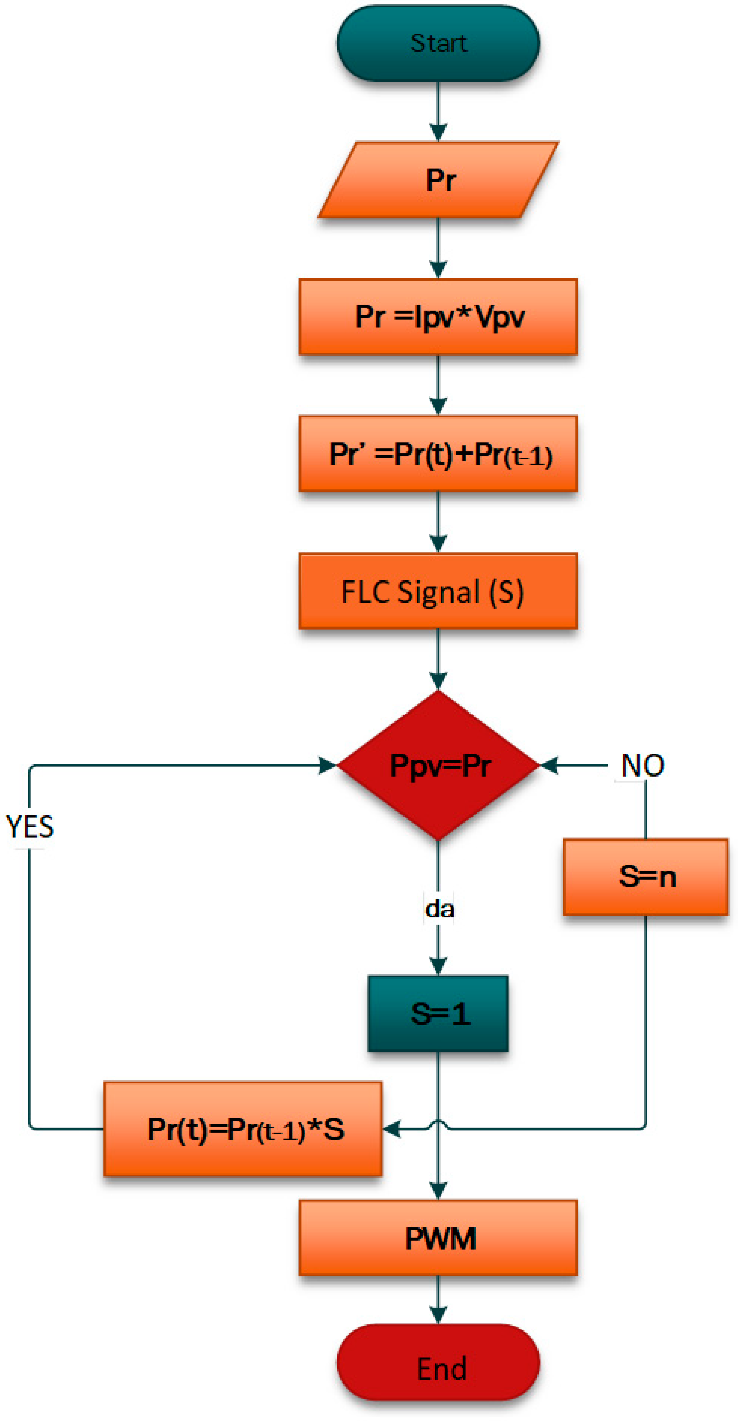
5.2. Optimization Procedure

The inputs for the optimization procedure are as follows. There are known: the climate where the PV application is implemented and the utilization period (here, a yearly operation is assumed). Therefore, information about the average available solar irradiation during the period is known. The average electrical power to be provided during the period by the PV module is a choice.
The MPPT could be implemented based on the FLC controller. The FLC algorithm compares the actual power of the PV system (PPV) with the reference power (maximum one) (Pr)—estimated value, via the FLC controller, at equal time intervals. The output of the FLC controller can direct the reference power to a new value, which is added to the previous value of each interval. The power highest value can be considered as the maximum one. The output from the FLC controller is routed to a PWM signal (Pulse Width Modulation) to control the operating cycle of the DC-DC voltage converter. This device raises the voltage to a value at which the PV system can operate at full power. The FLC-based MPPT technique was implemented based on the Fuzzy tool from MATLAB/Simulink. The first step is to define the FLC parameters (inputs, outputs) and methods (fuzzification and defuzzification) in the FIS (Fuzzy Inference System) editor.
After creating of the FLC controller in the MATLAB/Simulink, based on the FLC algorithm, we made the controller configuration for each component of the PV system. In Figure 16 is shown the diagram of the MPPT—FLC controller, where we have: PPV—actual power of the PV system, IPV—the current in the system, VPV—the system voltage, Pr—the maximum estimated reference power, and S—the FLC signal. In Figure 17 is presented the logic diagram for implementing the control algorithm MATLAB/Simulink; the input to the FLC controller is determined by the estimated reference power (Pr) and PV system actual power (PPV), while the output from the FLC is determined by the command signal (S).

5.3. Comparatives Analyze of Four Types of MPPT Algorithms

The authors proposed a comparative analysis based on MATLAB/Simulink work environment regarding four algorithms (FLC, P&O, IncCond and RC) for optimizing the maximum power point in order to choose the best algorithm. As expected, the FLC algorithm returned the best performances and gave evidence of increased accuracy, updated algorithm by adding two more operating points (since the FLC algorithm was the winner, in Section 5.1.1, only its model is presented). For modeling and numerical simulation, the use of an industrial photovoltaic module was considered (electrical characteristics are presented in Section 4). In order to determine the maximum power point for different solar irradiance values, the average irradiance values with a 20-minute acquisition step over a three-hour period were considered, namely: 843, 625, 756, 412, 530, 600, 821, 867, 917 W/m2. The temperature considered for modeling and numerical simulation of the electrical characteristics of the PV module was constant and had the value of 43 °C according to the manufacturer’s specifications. In Figure 18 and Figure 19, the I-V and P-V characteristics were obtained, respectively, with the corresponding maximum power points. It is notable that the FLC algorithm obtained the highest value for the maximum power point, which makes it feasible for the study of the partial shading of the respective PV panel for the optimization of its output power.

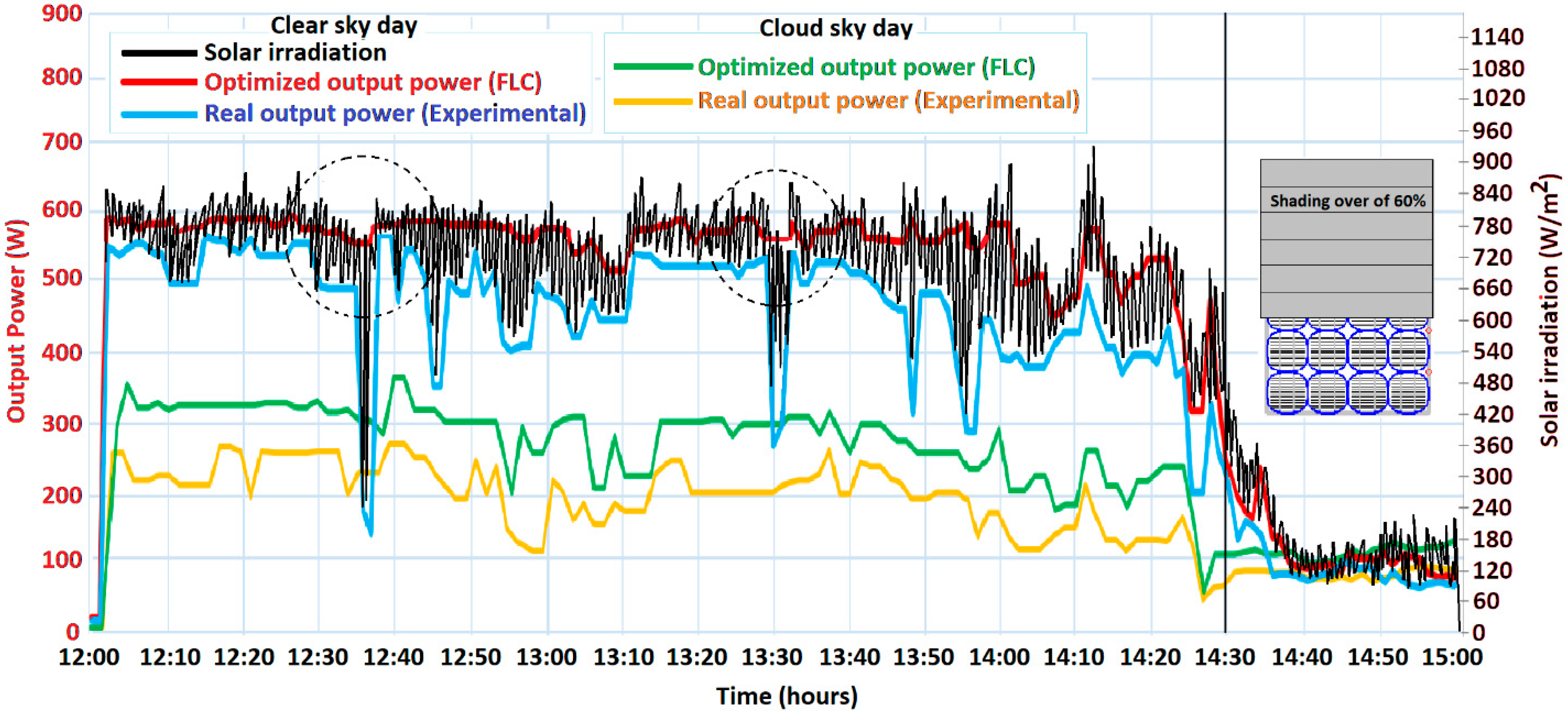
5.4. Response of the MPPT-FLC Technique to Partial Shading Conditions vs. Real Conditions

The results obtained from the modelling and simulation in the MATLAB/Simulink of the FLC controller based on MPPT show an increase in the power of the PV device. These findings are plotted with respect to the power of the PV generator. To highlight the contribution of FLC—MPPT for a clear sky day compared with the version of MPPT FLC for partially cloud sky day, the authors of the study analyzed the performance of the PV device. In order to plot the experimental data of the power curves (blue and yellows ones from Figure 20) comparison with the simulated data was performed; the field experiments was performed in August 2022 in Constanza City located in the South-East of Romania for two different types of days (clear sky day and partially cloudy sky day) were considered.
Figure 20 shows the power behavior of the photovoltaic generator. The results based on this optimized FLC algorithm for five operating points are presented in this Figure. We can see that the maximum value of the power is around 560 W using the experimental data obtained for two cases, namely: (1) a clear sky and (2) a partial cloudy sky. If we would analyze the results, we could see that the shading was considered. The results indicate a poor efficiency when the PV generator is affected by shading. Moreover, for a shading over 60%, the PV generator recorded a low power, correspondingly, a drastically negative influence on the efficiency and performances. After using the FLC controller based on MPPT, the power value of the PV generator rises to a maximum value (peak) of about of 590 W for clear sky day and 360 W for a partially cloudy sky, unfortunately, an excessive shading cannot be controlled.
For an adequate analysis, the comparison between real output power (experimental) and optimized output power based on MPPT-FLC is highlighted in Figure 20 with emphasis on the power gain in the case of the PV generator.
It can be remarked that, in the case of both characteristics, the curve obtained by numerical modeling is very close to the experimental curve, which indicates the accuracy of the model (FLC algorithm based on five-point operation), correspondingly, the accuracy of the MATLAB/Simulink working environment.
It could be remarked (see the dotted markers) that with sudden variations in solar irradiance due to the shading, the optimization based on the FLC algorithm keeps the output power constant, thus ensuring an excellent performance.

6. Validation of the Authors Study with Literature Results. Comparison with Other Approaches

A comparison of the authors study based on different approaches, methods, algorithms, and techniques technique with literature results regarding the extracted maximum power from PV systems is given in Table 3. It is stressed the novel results of the present article with the significant results obtained by the specialized literature.
At the same time, Table 3 presents a qualitative and quantitative comparison between literature and the results obtained in this paper (there were assigned as “Ref 0”); there were distinguished from other references that contain notable results presented by the authors of the published articles.
The most significant results obtained by the authors of specialized literature are numerically presented in Table 3. This comparison allows to the reader to identify much more easily and efficiently the effects of the results of the authors article as well as the notable published results obtained by various researchers. For an effective identification and correlation of the comparative results presented in Table 3, the following approach was developed: (1) Presentation of the method, (2) Degree of novelty from a qualitative point of view, and (3) Efficiency of the models/methods from a quantitative point of view.

7. Conclusions

We have proposed a complete method of optimizing photovoltaic modules, which uses a series parallel approach to determine the influence of temperature and shading effect to PV device. However, this study led to improving the output electrical parameters, making it possible to respond appropriately to sudden variations in solar radiation. We have analyzed the influence of the FLC controller on the output power of a photovoltaic generator in terms of power operational optimization. The obtained results can be developed and widely applied, both for complex stand-alone photovoltaic generators and on-grid ones. This research was dedicated to defining a special concept for extraction of the maximum power from a PV generator based on optimized FLC algorithm and the five-point operation, which determines a better accuracy. The authors modeled and simulated the PV generator for determining and tracking the maximum power point, along with operational optimization based on the MPPT-FLC controller.
The results show that a significant amount of additional energy can be extracted from a photovoltaic generator by applying a “tracker” to “track” the maximum power point based on FLC algorithm. At the same time, these results indicate an improved efficiency of the PV generator, during periods of low solar radiation or partially shading.
The simulations show that the derived model is correct. When the irradiance level is changed, the percentage increase in the maximum power point (MPP) is almost equal to the percentage increase in the incident irradiance level on the panel. In addition, the bypass diodes considered in the simulation approach achieve higher MPP values during partial shading. However, the maximum power point tracking (MPPT) based on FLC algorithm remains “stuck” to a local maximum instead of the global maximum.
The proposed FLC controller would show more robustness in terms of its dynamic behavior under different operating conditions and could successfully overcome the difficulties presented in non-uniform conditions, under partially shading.
The MPPT-based FLC could be applied to different types of solar cells (such as perovskite, tandem heterojunction with metal oxides, organic, dye sensitive, etc.) MATLAB/Simulink would allow the utilization of different types of solar cells and PV module configurations for the PV generator developed within the MPPT-FLC approach.

Author Contributions

Conceptualization, D.C.; methodology, D.C. and L.F.; formal analysis, D.C.; investigation, D.C. and L.F.; funding acquisition, L.F.; software, D.C..; validation, L.F. and D.C.; resources, L.F. and D.C.; data curation, L.F.; writing original draft preparation, D.C and L.F.; writing—review and editing, L.F.; visualization, L.F.; supervision, L.F.; project administration, L.F. All authors have read and agreed to the published version of the manuscript.

Funding

This work has been funded by the European Social Fund from the Sectorial Operational Programme Human Capital 2014–2020, through the Financial Agreement with the title “Training of PhD students and postdoctoral researchers in order to acquire applied research skills—SMART”, Contract no. 13530/16.06.2022-SMIS code: 153734.

Acknowledgments

This work has been supported by Polytechnic University of Bucharest, Faculty of Mechanics Engineering and Mechatronics through European Social Fund from the Sectorial Operational Programme Human Capital 2014–2020, through the Financial Agreement with the title “Training of PhD students and postdoctoral researchers in order to acquire applied research skills—SMART”, Contract no. 13530/16.06.2022-SMIS code: 153734.

Conflicts of Interest

The authors declare no conflict of interest.

Abbreviations

PV PhotovoltaicΔCExit membership
MPPT Maximum Power Point TrackingColdold disturbance
P&O Perturb and observePrreference power
RCRipple correlationIncCondIncremental Conductance
ACAlternative CurrentPPVactual power
DCDirect CurrentPLconsumer power
I-VCurrent-Voltage characteristicsWpwatt peak
P-VPower-Voltage characteristicsSaslope
FLCFuzzy Logic ControllerPWMPulse Width Modulation
FISFuzzy Inference SystemFFfilling factor
FLFuzzy LogicIBbattery current
MFMember FunctionVLdactual load voltage
NBLarge NegativeILload current
NSLow NegativeScommand signal
PSSmall PositiveIscshort circuit current
PBLarge PositiveVocopen circuit voltage
ZOZeroPmaxmaximum power
NMMedium Negative I”reference current
PMMedium Positive

References

  1. Fara, L.; Craciunescu, D.; Fara, S. Numerical Modelling and Digitalization Analysis for a Photovoltaic Pumping System Placed in the South of Romania. Energies 2021, 14, 2778. [Google Scholar] [CrossRef]
  2. Ongsakul, W.; Dieu, V.N. Artificial Intelligence in Power System Optimization; Informa: London, UK, 2016. [Google Scholar]
  3. Amin, A.A.E.; Al-Maghrabi, M.A. The Analysis of Temperature Effect for mc-Si Photovoltaic Cells Performance. Silicon 2018, 10, 1551–1555. [Google Scholar] [CrossRef]
  4. Fara, L.; Craciunescu, D. Output Analysis of Stand-Alone PV Systems: Modeling, Simulation and Control, Sustainable Solutions for Energy and Environment. Energy Procedia 2017, 112, 595–605. [Google Scholar] [CrossRef]
  5. Kurukuru, V.S.B.; Blaabjerg, F.; Khan, M.A.; Haque, A. A Novel Fault Classification Approach for Photovoltaic Systems. Energies 2020, 13, 308. [Google Scholar] [CrossRef] [Green Version]
  6. Martínez, F.; Lorenzo, E.; Muñoz, J.; Moretón, R. On the testing of large PV arrays. Prog. Photovolt. Res. Appl. 2012, 20, 100–105. [Google Scholar] [CrossRef] [Green Version]
  7. Craciunescu, D.; Fara, L.; Sterian, P.; Bobei, A.; Dragan, F. Optimized Management for Photovoltaic Applications Based on LEDs by Fuzzy Logic Control and Maximum Power Point Tracking. In Nearly Zero Energy Communities; Springer Proceedings in Energy; Springer International Publishing: Cham, Switzerland, 2018; pp. 317–336. [Google Scholar] [CrossRef]
  8. Fichera, A.; Pluchino, A.; Volpe, R. From self-consumption to decentralized distribution among prosumers: A model including technological, operational, and spatial issues. Energy Convers Manag. 2020, 217, 112932. [Google Scholar] [CrossRef]
  9. Luthander, R.; Widén, J.; Munkhammar, J.; Lingfors, D. Self-consumption enhancement and peak shaving of residential photovoltaics using storage and curtailment. Energy 2016, 112, 221–231. [Google Scholar] [CrossRef]
  10. Huang, P.; Lovati, M.; Zhang, X.; Bales, C.; Hallbeck, S.; Becker, A.; Bergqvist, H.; Hedberg, J.; Maturi, L. Transforming a residential building cluster into electricity prosumers in Sweden: Optimal design of a coupled PV-heat pump-thermal storage-electric vehicle system. Appl. Energy 2019, 255, 113864. [Google Scholar] [CrossRef]
  11. Chen, Y.; Wu, Y.; Song, C.; Chen, Y. Design, and implementation of energy management system with fuzzy control for DC microgrid systems. IEEE Trans. Power Electron. 2013, 28, 1563–1570. [Google Scholar] [CrossRef]
  12. Baniasadi, A.; Habibi, D.; Al-Saedi, W.; Masoum, M.A.; Das, C.K.; Mousavi, N. Mousavi Optimal sizing design and operation of electrical and thermal energy storage systems in smart buildings. J. Energy Storage 2020, 28, 101186. [Google Scholar] [CrossRef]
  13. Bozorgavari, S.A.; Aghaei, J.; Pirouzi, S.; Nikoobakht, A.; Farahmand, H.; Korpås, M. Robust planning of distributed battery energy storage systems in flexible smart distribution networks: A comprehensive study. Renew. Sustain. Energy Rev. 2020, 123, 109739. [Google Scholar] [CrossRef]
  14. Sameti, M.; Haghighat, F. Integration of distributed energy storage into net-zero energy district systems: Optimum design and operation. Energy 2018, 153, 575–591. [Google Scholar] [CrossRef]
  15. Parra, D.; Norman, S.A.; Walker, G.S.; Gillott, M. Optimum community energy storage system for demand load shifting. Appl. Energy 2016, 174, 130–143. [Google Scholar] [CrossRef]
  16. Sardi, J.; Mithulananthan, N.; Hung, D.Q. Strategic allocation of community energy storage in a residential system with rooftop PV units. Appl. Energy 2017, 206, 159–171. [Google Scholar] [CrossRef]
  17. Huang, P.; Lovati, M.; Zhang, X.; Bales, C. A coordinated control to improve performance for a building cluster with energy storage, electric vehicles, and energy sharing considered. Appl. Energy 2020, 268, 114983. [Google Scholar] [CrossRef]
  18. Huang, P.; Zhang, X.; Copertaro, B.; Saini, P.K.; Yan, D.; Wu, Y.; Chen, X. A technical review of modeling techniques for urban solar mobility: Solar to buildings, vehicles, and storage (S2BVS). Sustainability 2020, 12, 7035. [Google Scholar] [CrossRef]
  19. Cole, W.J.; Frazier, A. Cost Projections for Utility-Scale Battery Storage; National Renewable Energy Lab. (NREL): Golden, CO, USA, 2019.
  20. Diaconu, A.; Craciunescu, D.; Fara, L.; Sterian, P.; Oprea, C.; Fara, S. Estimation of electricity production for a photovoltaic park using specialized advanced software. In Proceedings of the ISES EuroSun 2016 Conference, Palma de Mallorca, Spain, 11–14 October 2016; pp. 1180–1182. [Google Scholar]
  21. Fara, L.; Craciunescu, D.; Diaconu, A. Results in performance improvement and operational optimization of photovoltaic components and systems. Ann. Acad. Rom. Sci. Ser. Phys. Chem. Sci. 2017, 2, 7–30. [Google Scholar]
  22. Diaconu, A.; Fara, L.; Sterian, P.; Craciunescu, D.; Fara, S. Results in sizing and simulation of PV applications based on different solar cell technologies. J. Power Energy Eng. 2017, 5, 63–74. [Google Scholar] [CrossRef] [Green Version]
  23. Theocharides, S.; Makrides, G.; Georghiou, G.E.; Kyprianou, A. Machine Learning Algorithms for Photovoltaic System Power Output Prediction. In Proceedings of the 2018 IEEE International Energy Conference (ENERGYCON), Limassol, Cyprus, 3–7 June 2018. [Google Scholar]
  24. Sebbagh, T.; Kelaiaia, R.; Zaatri, A. An experimental validation of the effect of partial shade on the I-V characteristic of PV panel. Int. J. Adv. Manuf. Technol. 2018, 96, 4165–4172. [Google Scholar] [CrossRef]
  25. Rezazadeh, S.; Moradzadeh, A.; Pourhossein, K.; Mohammadi-Ivatloo, B.; Márquez, F.G. Photovoltaic array reconfiguration under partial shading conditions for maximum power extraction via knight’s tour technique. J. Ambient. Intel. Human Comput. 2022, 14, 1–23. [Google Scholar] [CrossRef]
  26. How Digital Twin Technology is Changing the Solar Power. 2020. Available online: www.pratititech.com (accessed on 20 October 2022).
  27. Youssefa, A.; El-Telbanya, M.; Zekryb, A. The role of artificial intelligence in photovoltaic systems design and control: A review. Renew. Sustain. Energy Rev. 2017, 78, 72–79. [Google Scholar] [CrossRef]
  28. Mellit, A. Sizing of photovoltaic systems: A Review. Rev. Energ. Renouvelables 2007, 10, 463–472. [Google Scholar]
  29. Digital Platform. 2020. Available online: https://www.record-evolution.de/ (accessed on 20 October 2022).
  30. Craciunescu, D. Contributions to Development and Integration of Complex Photovoltaic Systems in Optoelectronic and Power Applications. Ph.D. Thesis, Polytechnic University of Bucharest, Bucharest, Romania, 2019. [Google Scholar]
  31. Singh, S.; Gupta, S.; Mathew, L. Simscape Based Modeling and Simulation of Solar Cell Module with Partial Shading Effect. Int. J. Mod. Electron. Commun. Eng. (IJMECE) 2013, 1. [Google Scholar]
  32. Ping, W.; Hui, D.; Changyu, D.; Shengbiao, Q. An Improved MPPT Algorithm Based on Traditional Incremental Conductance Method. In Proceedings of the 2011 4th International Conference on Power Electronics Systems and Applications, Hong Kong, China, 8–10 June 2011. [Google Scholar]
  33. Shiau, J.K.; We, Y.C.; Lee, M.Y. Fuzzy Controller for a Voltage-Regulated Solar-Powered MPPT System for Hybrid Power System Applications. Energies 2015, 8, 3292–3312. [Google Scholar] [CrossRef] [Green Version]
  34. Essefi, R.M.; Souissi, M.; Abdallah, H.H. Maximum Power Point Tracking Control Using Neural Networks for Standalone Photovoltiac Systems. Int. J. Mod. Nonlinear Theory Appl. 2014, 3, 53–65. [Google Scholar] [CrossRef] [Green Version]
  35. Mallika, S.; Saravanakumar, R. Genetic Algoritms Based MPPT Controller for Photovoltaic Sustems. Int. Electr. Eng. J. (IEEJ) 2014, 4, 1159–1164. [Google Scholar]
  36. Zhang, H. Constant Voltage Control on DC Bus of PV System with Flywheel Energy Storage Source (FESS). Int. Conf. Adv. Power Syst. Autom. Prot. 2011, 3, 1723–1727. [Google Scholar]
  37. Sharma, D. Designing and Modeling Fuzzy Control Systems. Int. J. Comput. Appl. 2011, 16, 975–987. [Google Scholar] [CrossRef]
  38. Letting, L.K.; Josiah, L.; Munda, Y. Optimization of Fuzzy Logic Controller Design for Maximum Power Point Tracking in Photovoltaic Systems. In Soft Computing in Green and Renewable Energy Systems; Springer: Berlin/Heidelberg, Germany, 2011; Volume 269, pp. 233–260. [Google Scholar]
  39. Atsu, D.; Dhaundiyal, A. Effect of Ambient Parameters on the Temperature Distribution of Photovoltaic (PV) Modules. Resources 2019, 8, 107. [Google Scholar] [CrossRef] [Green Version]
  40. Omar, M. Comparison between the Effects of Different Types of Membership Functions in Fuzzy Logic Controller Performance. Int. J. Eng. Res. Technol. 2015, 3, 2349–2355. [Google Scholar]
  41. Ali, A. Investigation of MPPT Techniques Under Uniform and Non-Uniform Solar Irradiation Condition–A Retrospection. IEEE Access 2020, 8, 127368–127392. [Google Scholar] [CrossRef]
  42. Sundarabalan, C.K.; Selvi, K.; Sakeenathul, K. Performance Investigation of Fuzzy Logic Controlled MPPT for Energy Efficient Solar PV Systems. In Power Electronics and Renewable Energy Systems; Springer: New Delhi, India, 2015; pp. 761–770. [Google Scholar]
  43. Mohapatra, A.; Nayak, B.; Das, P.; Kanungo Mohanty, B. A review on MPPT techniques of PV system under partial shading condition. Renew. Sustain. Energy Rev. 2017, 80, 854–867. [Google Scholar] [CrossRef]
  44. Karami, N.; Moubayed, N.; Outbib, R. General review, and classification of different MPPT Techniques. Renew. Sustain. Energy Rev. 2017, 68 Pt 1, 1–18. [Google Scholar] [CrossRef]
  45. Shams El-Dein, M.Z.; Kazerani, M.; Salama, M.M.A. Optimal photovoltaic array reconfiguration to reduce partial shading losses. IEEE Trans. Sustain. Energy 2013, 4, 145–153. [Google Scholar] [CrossRef]
  46. Gielen, D.; Boshell, F.; Saygin, D. The role of renewable energy in the global energy transformation. Energy Strategy Rev. 2019, 24, 38–50. [Google Scholar] [CrossRef]
  47. Niazi, K.A.; Yang, Y.; Nasir, M.; Sera, D. Evaluation of interconnection configuration schemes for PV modules with switched-inductor converters under partial shading conditions. Energies 2019, 12, 2802. [Google Scholar] [CrossRef] [Green Version]
  48. Kreft, W.; Filipowicz, M.; Odek, M. Reduction of electrical power loss in a photovoltaic chain in conditions of partial shading. Opt. Int. J. Light Electron. Opt. 2019, 202, 163559. [Google Scholar] [CrossRef]
  49. Ramalu, T.; Mohd Radzi, M.A.; Mohd Zainuri, M.A.A.; Abdul Wahab, N.I.; Abdul Rahman, R.Z. A Photovoltaic-Based SEPIC Converter with Dual-Fuzzy Maximum Power Point Tracking for Optimal Buck and Boost Operations. Energies 2016, 9, 604. [Google Scholar] [CrossRef]
  50. Dubey, S.; Narotam, J.; Seshadri, S.B. Temperature Dependent Photovoltaic (PV) Efficiency and Its Effect on PV Production in the World—A Review. Energy Procedia 2013, 33, 311–321. [Google Scholar] [CrossRef] [Green Version]
  51. Brito, M.A.G.; Galotto Sampaio, L.P.; Luigi, G.; Melo, A.; Canesin, C.A. Evaluation of the Main MPPT Techniques for Photovoltaic Applications. IEEE Trans. Ind. Electron. 2013, 60, 1156–1167. [Google Scholar] [CrossRef]
  52. Brito, M.A.G.; Sampaio, L.P.; Luigi, G.; Melo, G.A.; Canesin, C.A. Comparative analysis of MPPT techniques for PV applications. In Proceedings of the 2011 International Conference on Clean Electrical Power (ICCEP), Ischia, Italy, 14–16 June 2011; pp. 99–104. [Google Scholar] [CrossRef]
  53. Femia, N.; Petrone, G.; Spagnuolo, G.; Vitelli, M. Optimizing sampling rate of P&O MPPT technique. In Proceedings of the 2004 IEEE 35th Annual Power Electronics Specialists Conference (IEEE Cat. No.04CH37551), Aachen, Germany, 20–25 June 2004; Volume 3, pp. 1945–1949. [Google Scholar] [CrossRef]
  54. Tubniyom, C.; Jaideaw, W.; Chatthaworn, R.; Suksri, A. Effect of partial shading patterns and degrees of shading on Total Cross-Tied (TCT) photovoltaic array configuration. Energy Procedia 2018, 153, 35–41. [Google Scholar] [CrossRef]
  55. Guoqian, L.; Samuel, B.; Tseng, M.L.; Wang, C.H.; Liu, Y.; Li, L. Photovoltaic Modules Selection from Shading Effects for Different Materials. Symmetry 2020, 12, 2082. [Google Scholar] [CrossRef]
  56. Galeano, A.G.; Bressan, M.V.F.; Alonso, J.C. Shading Ratio Impact on Photovoltaic Modules and Correlation with Shading Patterns. Energies 2018, 11, 852. [Google Scholar] [CrossRef]
  57. Algarín, C.R.; Giraldo, J.T.; Álvarez, O.R. Fuzzy Logic Based MPPT Controller for a PV System. Energies 2017, 10, 2036. [Google Scholar] [CrossRef] [Green Version]
  58. Zhao, Q.; Shao, S.; Lu, L.; Liu, X.; Zhu, H. A New PV Array Fault Diagnosis Method Using Fuzzy C-Mean Clustering and Fuzzy Membership Algorithm. Energies 2018, 11, 238. [Google Scholar] [CrossRef] [Green Version]
  59. Simoes, M.G.; Franceschetti, N.N.; Friedhofer, M. A fuzzy logic based photovoltaic peak power tracking control. In Proceedings of the IEEE International Symposium on Industrial Electronics, ISIE ’98, Pretoria, South Africa, 7–10 July 1998; Volume 1, pp. 300–305. [Google Scholar]
  60. Quaschning, V.; Hanitsch, R. Numerical simulation of current–voltage characteristics of photovoltaic systems with shaded solar cells. Sol. Energy 1996, 56, 513–520. [Google Scholar] [CrossRef]
  61. Bishop, J. Computer simulation of the effects of electrical mismatches in photovoltaic cell interconnection circuits. Sol. Cells 1988, 25, 73–89. [Google Scholar] [CrossRef]
  62. Gautam, N.K.; Kaushika, N.D. Reliability evaluation of solar photovoltaic arrays. Sol. Energy 2002, 72, 129–141. [Google Scholar] [CrossRef]
  63. Lasnier, F.; Ang, T.G. Photovoltaic Engineering Handbook; Adam Hilger: Bristol, UK, 1990. [Google Scholar]
  64. Craparo, J.C.; Thacher, E.F. A solar–electric vehicle simulation code. Sol. Energy 1995, 55, 221–234. [Google Scholar] [CrossRef]
  65. Badescu, V.; Landsberg, P.T.; Dinu, C. Thermodynamic optimisation of non-concentrating hybrid solar converters. J. Phys. D Appl. Phys. 1996, 29, 246–252. [Google Scholar] [CrossRef]
  66. Khouzam, K.; Hoffman, K. Real-time simulation of photovoltaic modules. Sol. Energy 1996, 56, 521–526. [Google Scholar] [CrossRef]
  67. Badescu, V. Simple optimization procedure for silicon-based solar cell interconnection in a series–parallel PV module. Energy Convers. Manag. 2006, 47, 1146–1158. [Google Scholar] [CrossRef]
  68. Hassan, S.Z.; Li, H.; Kamal, T.; Arifoğlu, U.; Mumtaz, S.; Khan, L. Neuro-Fuzzy Wavelet Based Adaptive MPPT Algorithm for Photovoltaic Systems. Energies 2017, 10, 394. [Google Scholar] [CrossRef]
  69. Nabipour, M.; Razaz, M.; Seifossadat, S.; Mortazavi, S. A new MPPT scheme based on a novel fuzzy approach. Renew. Sustain. Energy Rev. 2017, 74, 1147–1169. [Google Scholar] [CrossRef]
  70. Bendib, B.; Krim, F.; Belmili, H.; Almi, M.F.; Boulouma, S. Advanced Fuzzy MPPT Controller for a Stand-alone PV System. Energy Procedia 2014, 50, 383–392. [Google Scholar] [CrossRef] [Green Version]
  71. Zadeh, L.A. Toward a theory of fuzzy information granulation and its centrality in human reasoning and fuzzy logic. Fuzzy Sets Syst. 2007, 90, 111–127. [Google Scholar] [CrossRef]
  72. Thambi, G.; Kumar, S.P.; Krishna, Y.M.; Aruna, M. Fuzzy-Logic-Controller-Based SEPIC Converter for MPPT in Standalone PV Systems. Int. Res. J. Eng. Technol. 2015, 2, 492–497. [Google Scholar]
  73. Ouil, D.S. Efefct of Different Membership Functions on Fuzzy Power System Stability for Synchronous Machine Connected to Infinite Bus. Int. J. Comput. Appl. 2013, 71, 975–985. [Google Scholar]
Figure 1. The shading effect on photovoltaic modules.
Energies 16 01169 g001
Figure 2. PV cell electrical model. S and D—photo-sensible and diode-type components of solar cell. Rs, Rsh—series and shunt resistance, respectively.
Energies 16 01169 g002
Figure 3. Electrical model of a simple series-parallel PV module. Rs,module, Rsh,module are series and shunt resistance, respectively.
Energies 16 01169 g003
Figure 4. PV generator test block diagram implemented in MATLAB/Simulink.
Energies 16 01169 g004
Figure 5. Plot representation of the temperature influence to the ISC characteristics of the PV generator.
Energies 16 01169 g005
Figure 6. Plot representation of the temperature influence to the VOC characteristics of the PV generator.
Energies 16 01169 g006
Figure 7. Plot representation of the temperature influence to the PMAX characteristics of the PV generator.
Energies 16 01169 g007
Figure 8. Plot representation of the temperature influence to the FF characteristics of the PV generator.
Energies 16 01169 g008
Figure 9. Current-Voltage characteristics under different partial shading conditions for series approach.
Energies 16 01169 g009
Figure 10. Power-Voltage (power characteristics) under different partial shading conditions for series approach.
Energies 16 01169 g010
Figure 11. Current-Voltage characteristics under different partial shading conditions for parallel approach.
Energies 16 01169 g011
Figure 12. Power-Voltage (power characteristics) under different partial shading conditions for parallel approach.
Energies 16 01169 g012
Figure 13. Fuzzy Block diagram.
Energies 16 01169 g013
Figure 14. Exit membership ΔC.
Energies 16 01169 g014
Figure 15. Power-Voltage characteristics of the PV panel with FLC based on 5 points of optimization.
Energies 16 01169 g015
Figure 16. MPPT-based FLC controller configuration.
Energies 16 01169 g016
Figure 17. Logic diagram for implementing the control algorithm in MATLAB.
Energies 16 01169 g017
Figure 18. Comparison between MPPT techniques for 4 algorithms regarding the MPP determination for I-V characteristics of an industrial PV module.
Energies 16 01169 g018
Figure 19. Comparison between MPPT techniques for 4 algorithms regarding the MPP determination for P-V characteristics of an industrial PV module.
Energies 16 01169 g019
Figure 20. Comparison between MPPT-FLC optimization output power and experimental data in terms of power gain for the whole PV generator.
Energies 16 01169 g020
Table 1. Electrical characteristics and performances of the PV module.
WATTROM H—M10-560
Description SymbolU.M.Values
Max. Power Pmax[W]560Energies 16 01169 i001
All Tolerance -[W]0 ± 5 W
Open circuit Voc[V]50.20
Short Circuit Isc[A]14.11
Max. Power Voltage Vmp[V]42.00
Max. Power Current Imp[A]13.35
Max System Voltage Pmax,system[VDC]1500
Max Series Fuse -[A]25
Nominal Operating Cell Temperature TN[°C]43 ± 2
Number of Cells Ncells[-]144
Table 2. FLC rules.
Table 2. FLC rules.
ColdSmallMediumHigh
Sa = dP/dV
Small NSNMNB
Small’ ZONSNM
Medium PSZONS
High’ PMPSZO
High PBPMPS
Table 3. Comparison of the results based on different investigation MPPT techniques/models/methods from literature with the results obtained by the authors of the present article.
Technique/Methods/ModelsRefNumerical Results and Efficiency of the Model/MethodNovelties of the Present Article and Other Articles From Literature
Temperature effect/Shading/MPPT/FLC/Method/Model/Investigation/Optimization0Module power output decreases by 20–30%—for about 50–60 °C. The power is optimized and stabilized to 590 W. The output power is increased with ~6%. Solar cells are used in the temperature range 5–50 °C. It was found that a temperature reduction of 3–9 °C could improve electrical performance with 7.2%.The present article was developed in order to unify the approach of the methods and models used for investigation of PV generator; in this way it was determined the influence of temperature and shading effects on performance of PV generator, also an optimization was implemented.
Temperature effect Method/Model/Investigation/Optimization3It was proved that PV module output power decreased by 0.8–0.9% for 1 °C temperature increase above the standard operating temperature. Keeping temperature at 20 °C, an increase of 9–12% in electrical yield is obtained.Solar cell performance decreases with increasing temperature, fundamentally owing to increased internal carrier recombination rates, caused by increased carrier concentrations. The operating temperature plays a key role in the photovoltaic conversion process.
This paper discussed the effect of light intensity and temperature on the performance parameters of monocrystalline and polycrystalline silicon solar devices. The performance and overview use of solar cells was expressed. The role of temperature on the electric parameters of solar cells has been studied. The experimental results showed that all electrical parameters of the solar cells, such as maximum output power, open circuit voltage, short circuit current, and fill factor have changed with temperature variation.
Shading effect Method/Model/Investigation/Optimization Shading effect on PV modules was simulated. Three standard configurations of PV array consisting of series-parallel (SP), bridge-linked (BL), and total cross-tied (TCT) were studied. 9 PV panels are arranged in 3 × 3 array.
45The shadow seriously affects the PV performance and the harvested power that can be obtained. Moreover, the authors proved that the partial shading contributes approximately with 20–25% to the efficiency reduction and also a hot spot in the corresponding PV module could cause severe damage to it.This study aimed to provide photovoltaic module selection with better performance in the shading conditions for improving production efficiency and reducing photovoltaic system investment cost through the symmetry concept, combining both mathematical and engineering principles of solar energy.
49Hence, the authors proposed the Differential Power Processing Technique (DPP) based on interconnection as a promising solution to enhance the energy yield for PV modules with minimal mismatch power losses during partial shading conditions. Thus, for this method, they obtain the minimum losses ~1.5%, taking into account interconnections.This paper presented the study of a simplified approach to model and analyze the performance of partially shaded photovoltaic modules using the shading ratio. This approach integrated the characteristics of shaded area and shadow opacity into the PV model.
56The authors found from simulations the following result: when shading is greater than or equal to 50% of the total area of solar PV module, the reconfiguration of solar PV arrays cannot increase the power output higher than 5%. Therefore, it is unnecessary to reconfigure the solar PV array. As for the cases of shaded area less than 50% of the total area, it is more suitable to reconfigure the solar PV array.This paper was dedicated on five-parameter modeling for photovoltaic systems. Additionally, a simulation for partial shading on the photovoltaic system was presented to illustrate a feasible assessment during the design of a PV system for loss of energy conversion due to shading.
MPPT techniques Comparison/Literature Review/Evaluation46The authors showed that for Particle Swarm Optimization (PSO) an efficiency enhancement of 12.19% compared with the P&O method, instead the Fuzzy Logic Control (FLC) presents an efficiency of about 15%. At the same time, FLC is very fast and very stable.In this paper, the concept of power tracking for PV systems was highlighted and an overview on 40 old and recent Maximum Power Point Tracking (MPPT) methods, available in the literature, was presented and classified. These methods were mathematically modeled and described in such a way the reader can select the most appropriate method for his own application. A comparative table was presented at the end of the paper to simplify the classification of different methods.
43The authors concluded that most of the conventional MPPT algorithms are useful to track the Global Maximum Power Point—GMPP under normal solar irradiance conditions but fails to obtain accurate GMPP under rapidly changing and partial shading conditions. However, hybrid optimization algorithms are fast and accurate in tracking the GMPP under partial shading and rapidly changing solar irradiance conditions. The tracking speed for one of hybrid optimization algorithm the Modified Hill-Climbing with Fuzzy Logic-Control (MHCL-FLC) is very fast, with an efficiency of up to 98~99% but this is based on a complex algorithm and it is quite difficult to implement this algorithm using embedded technologies.This article focused on classifications of online, offline, and hybrid optimization MPPT algorithms, under the uniform and non-uniform irradiance conditions. It summarized various MPPT methods along with their mathematical expression, operating principle, and block diagram/flow charts. This research will provide a valuable pathway to researchers, energy engineers and strategists for future research and implementation in the field of maximum power point tracking optimization.
54The analyzed methods were adjusted to provide its best performance with the same set of irradiation and temperature steps. In this context, the Ripple Correlation Beta-method stands with 98% of energy extracted, the P&O method reach 94% and Incremental Conductance (IC) stands at 92%. The author of this paper does not consider the FLC method of analysis.This paper presented a careful evaluation among the most usual MPPT techniques, doing meaningful comparisons with respect to the amount of energy extracted from the photovoltaic (PV) panel, PV voltage ripple, dynamic response and use of sensors; considered were the models first implemented via MATLAB/Simulink.
FLC algorithm
Fuzzy-logic-control
(FLC)
44The results showed that a significant amount of additional energy (approximately 7–9%) can be extracted from a photovoltaic generator by applying a “tracker” to “track” the maximum power point based on fuzzy logic. At the same time, these results indicated an improved efficiency of the PV generator, as the batteries could then be charged and used during periods of low solar radiation.This paper presented a new stable Fuzzy Logic Control (FLC) algorithm based on maximum power point tracking (MPPT) for stand-alone photovoltaic (PV) system. The proposed method used P-V variation as the input, which significantly simplified the computation.
33The proposed approach provides an energy efficiency of about 10–15% on the PV curve.The authors stated that in high solar insolation, FLC-MPPT algorithm suffered from drift because of the wrong decision taken by the algorithm. The paper presented a modified FLC-MPPT algorithm that avoids the drift in suddenly changing irradiance and accurately tracks the MPPT.
57The authors proved that the fuzzy controller has excellent performance when there are sudden changes in the operating temperature of the PV module, in contrast with P&O control, which is considerably affected, presenting power losses up to 46.18 W.The paper proposed a robust FLC-MPPT technique that used a second-order sliding mode control strategy. The results proved that the algorithm provided fast response and less chattering under varying atmosphere.
58Simulation analysis indicated that the diagnostic accuracy of the proposed method was 96%. Field experiments further verified the correctness and effectiveness of the proposed method, and the method can complete the PV array diagnosis.The paper presented a modified version of FLC-MPPT optimization. The results revealed that the proposed algorithm could track the global maximum, especially under the partial shading conditions.
38The authors determined that the lower energy losses obtained by the dual-FLC MPPT with only 2.5 µJ is compared to the single-FLC MPPT with 4.2 µJ. Interestingly, a large difference between both MPPTs can be seen during boost operation.The paper presented a fractional order control based FLC-MPPT algorithm. The results showed high tracking accuracy for remarkable climate changes.
71A rapid increase in irradiance from 1000 W/m2 to 1200 W/m2 within a time period of 2 s was simulated by the authors. The cell temperature was kept at a constant value of 25 °C. Under these operating conditions, the FLC-based MPPT method is more significant and shows how the power output of the FLC based MPPT increases linearly, whereas the conventional P&O MPPT technique determines a vast deviation from the MPPT.The proposed FLC-MPPT technique ensured the fast error tracking capability for PV pumping systems.
Disclaimer/Publisher’s Note: The statements, opinions and data contained in all publications are solely those of the individual author(s) and contributor(s) and not of MDPI and/or the editor(s). MDPI and/or the editor(s) disclaim responsibility for any injury to people or property resulting from any ideas, methods, instructions or products referred to in the content.

