A Hybrid Grey Wolf Assisted-Sparrow Search Algorithm for Frequency Control of RE Integrated System

Abstract

Nowadays, renewable energy (RE) sources are heavily integrated into the power system due to the deregulation of the energy market along with environmental and economic benefits. The intermittent nature of RE and the stochastic behavior of loads create frequency aberrations in interconnected hybrid power systems (HPS). This paper attempts to develop an optimization technique to tune the controller optimally to regulate frequency. A hybrid Sparrow Search Algorithm-Grey Wolf Optimizer (SSAGWO) is proposed to optimize the gain values of the proportional integral derivative controller. The proposed algorithm helps to improve the original algorithms’ exploration and exploitation. The optimization technique is coded in MATLAB and applied for frequency regulation of a two-area HPS developed in Simulink. The efficacy of the proffered hybrid SSAGWO is first assessed on standard benchmark functions and then applied to the frequency control of the HPS model. The results obtained from the multi-area multi-source HPS demonstrate that the proposed hybrid SSAGWO optimized PID controller performs significantly by 53%, 60%, 20%, and 70% in terms of settling time, peak undershoot, control effort, and steady-state error values, respectively, than other state-of-the-art algorithms presented in the literature. The robustness of the proffered method is also evaluated under the random varying load, variation of HPS system parameters, and weather intermittency of RE resources in real-time conditions. Furthermore, the controller’s efficacy was also demonstrated by performing a sensitivity analysis of the proposed system with variations of 75% and 125% in the inertia constant and system loading, respectively, from the nominal values. The results show that the proposed technique damped out the transient oscillations with minimum settling time. Moreover, the stability of the system is analyzed in the frequency domain using Bode analysis.

1. Introduction

Currently, rising energy demand and the depletion of fossil fuel resources have necessitated the extensive use of Renewable Energy (RE), which is considered clean and cost-effective, and likely to be connected to interconnected power systems for distributed utilization [1]. The integration of RE such as solar and wind leads to an uncertain variation in the generation of power due to the intermittent nature of RE, which introduces frequency oscillation that leads to multiple protection relays trip in the power system [2]. Automatic Load Frequency Control (ALFC) has proven very effective in regulating the system frequency by adjusting the generation system. Hence, the overall generation matches the load demand to successfully operate the interconnected power networks. To achieve this, a robust control technique is vital in each area of the interconnected power network to maintain the nominal system frequency within the prescribed limits of ±0.2 Hz and planned tie-line power exchange [3]. To study this, the system frequency and tie-line power exchange parameters are considered as Area Control Error (ACE), which serves as input to the controller [4].

For ALFC applications, researchers have developed numerous controllers in the past. A conventional Proportional-Integral (PI) controller is used to enhance the frequency stability of the power system using an electric vehicle as an energy storage unit [5]. In reference [6], a four-area multi-source thermal system is controlled using linear quadrat/linear Gaussian control. Usually, the conventional Proportional-Integral-Derivative (PID) controllers are the best option due to their extra degree of freedom, affordability, and simplicity when compared to more robust controllers such as the Sliding Mode Control (SMC) [7], the Model Predictive Controller (MPC) [8], and H2/H∞ controllers [9]. In reference [10], a hybrid fuzzy logic controller with sliding mode was implemented for a microgrid system to evaluate the penetration of Renewable Energy Resources (RERs) connected with a power system. Another hybrid controller based on PID with fuzzy logic technique has been evaluated for a microgrid system [11]. In this paper, the effect of designing high performance power converters has been demonstrated to achieve a stable power system. All these controllers are challenging to implement in real-time and need advanced mathematics to derive the control law [12]. On the other hand, tuning the parameters of the PID controller is critical for a large dynamic HPS model. Instability in the system may result from the improper tuning of the PID parameters, which displays poor dynamic response in the frequency regulation of the system. To resolve this, several papers have been published in the literature to optimize the gain values of the PID controller using Artificial Neural Network (ANN) [13] and Fuzzy Logic control (FLC) [14]. Despite their benefits, their application in the actual ALFC system is constrained by the computational time required to choose a rule foundation fuzzy logic and a big training database for ANN [15]. However, the selection has no precise mathematical meaning, which might occasionally result in poor ALFC performance.

On the other hand, numerous heuristic approaches are used to optimize the parameters of the PID controller for ALFC, as illustrated in

Table 1. Review of optimization algorithms used to study the ALFC.

Ref. No.	Controller Type	Optimization	Model Description	Limitations
[16]	PID	GWO	Two-area thermal system	GRC, GDB, and BD nonlinearities in thermal systems and RER have not been considered in this work. The most significant limitation of this optimization technique is trapping in local optimal points
[17]	PFMPID	GOA	Three-area multi-source power system comprises thermal, hydro, wind, diesel, and RFB with GDB and GRC	BD has not been considered in this study. Moreover, the GOA optimization search process begins with a population or flock of grasshoppers whose locations are comparable to design vectors which leads to poor exploration
[18]	PID	CTO	Two-area multi-source with thermal, hydro, and gas units in each area	Non-conventional power resources have not been considered in this study. The CTO algorithm has the drawback of a greater number of parameters to be initialized
[19]	PID	GWO	Single area multi-source power system comprises thermal, hydro, and gas units	RER has not been considered, and the limitation of GWO is that poor exploration leads to trapping in local optimal points
[15]	PID	Hybrid PSO-GSA	Considering a two-area thermal system with GRC and GDB	For a highly nonlinear and big dimensional system such as ALFC, PSO exhibits poor exploration and takes longer to find global minima. The PSO-GSA approach overcomes this, although the study considered only a conventional source
[20]	PID	MPA	Two-area multi-source systems were taken into consideration, with WTPG, STPP, BES, and thermal plants in area 2 as well as STPP, PV, SMES, and thermal power plants combining GDB and GRC in area 1, and a reheat generator with wind and PV RERs in area 2. GRC has been considered in the two-area	MPA’s main drawback is a slow convergence rate with poor exploration ability
[21]	PID	HIO	Two-area reheat turbine power plant with gas and hydro units in each area	RER has not been considered in this study
[22]	PID	DE	Two-area multi-source with hydro, thermal, and wind power plants in each area	Nonlinearities are not considered. The limitation of DE is inapplicable to solving many complex real-world problems in continuous domains
[23]	PIDA	MPA	Two-area non-reheat thermal system	This study has not considered RER, GRC, BD, or GDB
[24]	PID	WOA	Two-area reheat thermal system	Nonlinearities are not considered. The limitation of WOA is that whales are drawn to the coefficient vector during the later phases of WOA iteration convergence, and as a result, the whole whale population quickly enters the local optimum for the high-dimensional optimization problem
[25]	PID	SSO	Two-area thermal system with GRC and GDB considered with the wind power plant in both the areas	The drawback of SSO is that the update rule fails when one of the dimensions has a lower bound other than zero

. PID or other modified forms of PID controllers for ALFC applications, the system model considered, the recent optimization algorithms used, and the limitations of the control method are briefly depicted in Table 1.

The optimization algorithm listed in Table 1 is an individual metaheuristic algorithm. Individual algorithms are advantageous due to their minimum requirements for function evaluation and ease of usage throughout the whole optimization process. However, the probability of local optima stagnation is very high, and individual meta-heuristic algorithms have difficulty in balancing between exploration and exploitation in order to find the global optima [26]. To cater to this issue, various modifications are performed in meta-heuristic algorithms to enhance their performance. One of the most recent and popular methods is to apply chaos theory in meta-heuristic algorithms to improve the global convergence speed and exploration/exploitation capabilities of optimization algorithms, resulting in more diversity in solutions. Another way is by hybridizing two algorithms.

Hybrid algorithms have recently been a popular topic applied in several domains [27,28,29,30]. Combining the qualities and features of two different algorithms would provide an optimization tool that is more dependable and potent for solving complex problems. It is recognized that combining evolutionary algorithms can increase their performances with problem-dependent local searches [31]. In recent years, numerous swarm intelligence optimization algorithms have been proposed and investigated in the literature, such as the Ant Colony Optimization (ACO) [32], Manta-Ray Foraging Optimizer (MRFO) [33], Salp Swarm Optimization (SSO) [34], SSA [35], and GWO [36]. Among them, SSA is a new optimization intelligence algorithm proposed in 2020 [35] that mimics the foraging behavior of sparrows to tackle particular optimization problems. SSA is distinct from other intelligent optimization algorithms by its high search accuracy, quick convergence time, superior stability, and robustness [36]. However, in the later stages of convergence, SSA is prone to local optima due to poor exploitation [37]. These issues directly impact SSA’s optimization effect, resulting in the inability to discover the optimal global solution.

Another popular swarm intelligence algorithm is GWO, developed by Mirjalili et al. [36], which has received a great reception in the optimization field. This algorithm simulates the natural hunting and dominance behavior of grey wolves. GWO has received great attention because of its simplicity and ease of implementation, and it has been used to tackle many real-time optimization problems. However, when handling complex, high-dimensional, and unimodal problems, GWO can be stuck in local optima due to its poor exploration [37]. Hence, to improve the convergence speed and avoid the optima problems, GWO can be hybridized with a good exploration ability algorithm.

Therefore, based on the advantages and disadvantages of SSA and GWO, the hybrid method is the possible solution to eradicate the limitations and combine the advantages of the two algorithms. Hence, this paper attempts to hybridize SSA with GWO to balance the exploration and exploitation phases, improving the controller performance in terms of steady-state and dynamic responses for frequency and power flow variation in interconnected power systems. The main contributions of this research study are summarized as follows:

• A hybrid SSAGWO algorithm is proposed to improve the SSA algorithm exploitation ability, and the algorithm is tested using various classical benchmark functions to prove its effectiveness against other algorithms.
• Auto-tuning of the PID controller parameters for ALFC of an RER-integrated HPS network is implemented using various optimization algorithms to verify the robustness of the proposed algorithm.
• The proposed system is tested using the data of an actual solar power plant, emulated for extreme operating conditions.
• A stability analysis is conducted to prove the efficacy and robustness of the proposed technique.

The paper is organized as follows: Section 2 presents the mathematical modeling of the two-area power system considered in this study. Next, Section 3 discusses the control strategy for load frequency control of the two-area power system. Section 4 discusses in detail the formulation procedure of the proposed hybrid SSAGWO algorithm. The results and critical analysis of the obtained results are discussed in Section 5, and Section 6 concludes the paper.

2. System Model

The study proposed in this paper consists of a two-area reheat steam power turbine, Photovoltaic (PV), and Wind Turbine Power Generator (WTPG) conversion, as shown in Figure 1. The two-area power system consists of a governor, reheat power thermal turbine generators with 0.05% of Governor Dead Band (GDB) and 10% of Generator Rate Constraints (GRC), and Boiler Dynamics (BD). In this research, two symmetrical power generator areas have been proposed with the parameters shown in Appendix A [15,38]. The BD has been considered for the realistic two-area reheat power systems. The thermal power plant uses the boiler dynamics arrangement to generate steam under high pressure. The long-term process of the steam flow on the boiler drum is considered in this model as combustion control. The block diagram configuration of the BD is shown in Figure 2. Oil-fired boiler type parameters [39] are listed in Appendix A.

2.1. SPV Model

SPV cells comprising semiconductor materials can convert photon energy directly into electrical energy. Power loss is also modeled because of the boundary and external contact, represented by series resistors, and a leakage current, represented by parallel resistance. SPV power generation is intermittent and dependent on sun irradiation and temperature; thus, a random power source can represent SPV behavior [40]. The block diagram of the SPV is shown in Figure 3. The linearized SPV model, which is considered for the ALFC model, is given by [40]:

Where ∆T_PV is the time constant of the SPV, ∆P_Solar is the change in solar irradiation power, and ∆P_PV denotes the change in power generated from solar to the power system.

2.2. WTPG Model

The mathematical model implementation for the wind power plant comprises a hydraulic pitch actuator, data fit pitch response, and blade characteristics, as shown in Figure 4. The pitch angle control mechanism keeps the pitch angle at the desired value based on wind speed. Thus, wind turbine production may be controlled by adjusting the pitch angle regardless of wind speed. The wind’s mathematical modeling transfer function model can be given in [41]:

Where ∆T_WT is the time constant of the wind turbine, ∆P_Wind is the change in wind speed, and ∆P_W is the change in power generated by the power system.

2.3. RFB Structure

RFB is a type of electrochemical energy storage compensation device that can convert energy from its electrical form to its chemical form and vice versa through electrochemical reaction processes [42]. RFB is an efficient method for reducing frequency deviations and tie-line power and is considered a fast active power compensation energy device. The RFB block diagram model integrated with areas 1 and 2 is shown in Figure 5 [41]:

Where T_RFB and K_RFB are the time and gain constant of the RFB. The main objective of the RFB is to charge and store energy from the power system as a very small load during a normally operating system, and it delivers the stored energy to the interconnected power system during any sudden change in load to reduce frequency fluctuations.

3. Control Strategy

The closed loop of the two-area power system can be simplified as shown in Figure 6:

Where ∆P_tie is the power deviation of the tie line of the power system. The transfer function of the PID controller is given by:

$$C(s)=k_p+\frac{k_i}{s}+s{k}_d$$

(1)

where k_p is the proportional gain, k_i is the integral gain, and k_d is the derivative gain. The PID controller output of the power system is as follows:

$$u_{1,2}=k_{p1}AC{E}_{1,2}+k_i{\displaystyle {\int }_0^{t}AC{E}_{1,2}dt+\frac{dAC{E}_{1,2}}{dt}}$$

(2)

The gain of the PID controller in this study is designed to minimize the steady-state error guides, such as the performance index ITAE as given below:

$$J=ITAE={\displaystyle {\int }_0^{t}t\left|AC{E}_i\right|dt={\displaystyle {\int }_0^{t}t\left\{\left|\Delta f_i+\Delta P_{tie,i-j}\right|\right\}}dt}$$

(3)

where i and j are the area numbers from 1,2,3, 4, …. n with i ≠ j.

This study aims to minimize J by tuning the values of PID controller parameters by using techniques such as the Z–N technique and intelligence optimization algorithms techniques such as PSO, GWO, SSA, and the proposed new hybrid SSAGWO.

4. Proposed Hybrid SSA-GWO

In this section, an effort was made to develop a new hybrid metaheuristic algorithm that combines the strength of swarm-inspired algorithms such as SSA with GWO to tune the values of the PID controller for a multi-area power system.

4.1. Grey Wolf Optimization

GWO is a well-known swarm intelligence optimization technique. The algorithm searches and optimizes by simulating the process of tracking, enclosing, and hunting, which was inspired by the predation behavior of the grey wolf population. There are various types of members in a wolf pack depending on the level of dominance, such as α, β, δ, and ω. The best three solutions are α, β, and δ, who leads the pack ω. The grey wolves hunt in a pack and collaborate to catch prey. The technique is to chase the prey and encircle it [43]. The mathematical model of the encircling behavior of grey wolves is in the following equations:

$$\overrightarrow{X}(t+1)=\frac{{\overrightarrow{X}}_1+{\overrightarrow{X}}_2+{\overrightarrow{X}}_3}{3}$$

(4)

$${\overrightarrow{X}}_1={\overrightarrow{X}}_{\alpha }(t)-\overrightarrow{A}\cdot {\overrightarrow{D}}_{\alpha },{\overrightarrow{X}}_2={\overrightarrow{X}}_{\beta }(t)-\overrightarrow{A}\cdot {\overrightarrow{D}}_{\beta },and{\overrightarrow{X}}_3={\overrightarrow{X}}_{\delta }(t)-\overrightarrow{A}\cdot {\overrightarrow{D}}_{\delta }$$

(5)

$${\overrightarrow{D}}_{\alpha }=\left|{\overrightarrow{C}}_1\cdot {\overrightarrow{X}}_{\alpha }-\overrightarrow{X}\right|,{\overrightarrow{D}}_{\beta }=\left|{\overrightarrow{C}}_2\cdot {\overrightarrow{X}}_{\beta }-\overrightarrow{X}\right|,and{\overrightarrow{D}}_{\delta }=\left|{\overrightarrow{C}}_3\cdot {\overrightarrow{X}}_{\delta }-\overrightarrow{X}\right|$$

(6)

$\overrightarrow{X}(t)$ represents the current position of the grey wolf; $\overrightarrow{A}$ is a coefficient vector; $\overrightarrow{D}$ represent the distance that varies according to the place of the prey ${\overrightarrow{X}}_p$; $\overrightarrow{a}$ is a factor that reduces from 2 to 0 linearly during optimization; ${\overrightarrow{r}}_1$ and ${\overrightarrow{r}}_2$ are random numbers between 0 and 1; $t$ represents as the current iteration, and T is the maximum iteration [44].

To predict the prey, we suppose that the best solution discovered so far (the alpha wolf) is the prey’s location because he is leading the pack and knows the prey’s location, while the second-best solution is for β wolf, and the third-best solution is δ wolf in the current iteration [45]. A is a random number in the gap $\left[-2a,2a\right]$. The wolves move to attack the prey when the value of $\left|A\right|<1$. Exploration is the ability to search for prey, while exploitation is the ability to attack the prey. The arbitrary values of A are used to force the wolves to move away from the prey. Furthermore, when the value of $\left|A\right|>1$, the wolves are forced to diverge from the prey (local minimum).

4.2. Sparrow Search Algorithm

The SSA is a swarm intelligence optimization technique. This technique mimics sparrow foraging behavior. It has three sorts of individual behavior: discoverer, follower, and investigator, and the sparrows update their locations according to their own rules. The discoverer searches for food and guides the rest of the community [35]. After discovering the discoverer’s location, followers search for food around this location. The follower’s location is updated according to Equation (7) [46,47]:

$$X_i^{t+1}=\left\{\begin{array}{ll}Q\cdot \exp (\frac{X_{worst}-X_i^t}{i^2}),\hfill & \hfill i>\frac{n}{2}\\ X_{best}^{t+1}+\left|X_i^t-X_{best}^{t+1}\right|\cdot A\cdot L,\hfill & \hfill i\le \frac{n}{2}\end{array}\right\}$$

(7)

where X_best represents the best individual position, which means the best current location; X_worst is the current worst global location; A is a d × d_matrix, which contains each factor randomly assigned 1 or −1; n represents the number of sparrows; when i ≤ n/2, it proposes the ith entrant is searching for food close to the best location, if i > n/2, it means the ith entrant needs to fly to another location for food.

Individuals from the population are chosen at random to be investigators. When predators attack, they send out signals that cause sparrows to flee to a safe location [46].

The mutation strategy in SSA directly affects convergence accuracy and speed. The SSA performs better in solving complex optimization problems but has the disadvantages of reduced population diversity and insufficient convergence accuracy. It could have a chance to fall into the local optimum, failing to achieve the optimum solution to the problems.

4.3. Proposed Optimization Algorithm

A new hybrid sparrow search algorithm based on the GWO, namely SSAGWO, is proposed in this paper. Its features allow the SSAGWO to avoid the local optimum while improving convergence speed and accuracy. The exploitation capability of the GWO is introduced into the sparrow search algorithm to improve its exploitation ability. The modification in the structure of SSA is improving the exploitation ability by using the behavior of exploration ability in GWO to compromise between exploitation and exploration. Improving the exploitation in SSA with the exploration effort should be achieved by hybridization between SSA and GWO. The variants of the position of SSA Equation (7) are mixed with the distance equation of GWO by new weight factor (θ) to keep the problem’s final solutions near the optimal values. The modification-guided equations are rewritten as follows:

$${\overrightarrow{D}}_{\alpha }=\left|{\overrightarrow{C}}_1\cdot {\overrightarrow{X}}_{\alpha }-\theta \overrightarrow{X}\right|,{\overrightarrow{D}}_{\beta }=\left|{\overrightarrow{C}}_2\cdot {\overrightarrow{X}}_{\beta }-\theta \overrightarrow{X}\right|,and{\overrightarrow{D}}_{\delta }=\left|{\overrightarrow{C}}_3\cdot {\overrightarrow{X}}_{\delta }-\theta \overrightarrow{X}\right|$$

(8)

The probability of shifting the position of all agents is calculated using Equation (9):

$$\mathsf{\Gamma }\left[X(t+1)-X(t)\right]=\left|\frac{\left[X(t+1)-X(t)\right]}{\sqrt{{\left[X(t+1)-X(t)\right]}^2+1}}\right|$$

(9)

where Γ is the probability factor. If the result of [X(t + 1) − X(t)] is positive, the sparrows select the food, while if the result is negative, the sparrows move far away from predators. It is worth noting that the correct position is quickly achieved by selecting well the boundaries of the PID factors. The SSAGWO’s specific steps are described in detail:

• Step 1: Initialize the sparrow search population and its parameters (n is the total number of sparrows, T_max maximum iteration, d is the number of variables).
• Step 2: While (t < T_max), rank the sparrows according to their fitness values by minimizing J in Equation (3). Find the current best value, which is the minimum fitness value, and the current worst value, which is the maximum fitness value.
• Step 3: Update the sparrow location for the discoverer by using Equation (10).

$$X_i^{t+1}=\left\{\begin{array}{ll}{X}_i^t\times \exp (\frac{-i}{\alpha \cdot T_{\max }}),\hfill & \hfill R_2<STh\\ X_i^t+Q\cdot L,\hfill & \hfill R_2\ge STh\end{array}\right\}$$

(10)

With $X={\left[X_1,X_2,X_3,\dots X_i\dots X_n\right]}^T,X_i=\left[X_{i,1},X_{i,2},X_{i,3}\dots X_{i,d}\right]$.

Where t denotes the current iteration; $X_i^t$ is the location of the ith sparrow at iteration t; α is a random number between 0 and 1; R₂ is the alarm value, which is 0 < R₂ ≤ 1; the safety threshold is STh, and it is valued 0.5 ≤ STh <1; L is a 1 × d_matrix; d_matrix is the matrix including 1 in each factor; and Q is a random value with a mean of zero and a variance of one that follows the normal distribution. If R₂ < STh, it indicates that the foraging surroundings are safe, while R₂ ≥ STh denotes that some individuals already have faced dangerous animals and that all sparrows must flee to other safe locations as soon as possible.

• Step 4: If the ith individuals at the current iteration are less or equal to half the sparrow population, then update the follower’s position using Equation (7) and go to step 9. Except for that, run the GWO algorithm.
• Step 5: Initialize the values of a, A, and C.
• Step 6: Calculate the first-best value of the alpha wolf, the second-best value of the beta wolf, and third best value of the gamma wolf.
• Step 7: Determine the distance between the wolves and prey using Equation (6). After that, calculate the value of the new position using Equations (4) and (5).
• Step 8: Export the position of the best three wolves and exchange it with the current sparrows. The flowchart of the SSAGWO is shown in Figure 7.
• Step 9: Update the follower’s position using Equation (7). Then, update the investigator’s location using Equation (11).

$$X_i^{t+1}=\left\{\begin{array}{ll}{X}_{best}^t+{\beta }_e\left|X_i^t-X_{best}^t\right|,\hfill & \hfill f_i>f_b\\ X_{best}^{t+1}+K\frac{\left|X_i^t-X_{best}^{t+1}\right|}{(f_i-f_w)+\epsilon },\hfill & \hfill f_i=f_b\end{array}\right\}$$

(11)

where β_e denotes the random step length control coefficient, which has a variance of 1 and a mean value of 0 and follows the normal distribution; K is a random number between −1 and 1; f_i is the fitness value of the ith individual; f_b is the current global best fitness; and f_w is the current global worst fitness.

• Step 10: By using Equation (9), if the probability factor is a positive value, calculate the fitness value using Equation (3) and compare it with the best fitness solution to obtain the minimum optimal value. However, if the probability factor is negative, go to step 5.

The parameters of the proposed SSAGWO algorithm technique are initialized at maximum iteration = 100, the number of search agents = 50, and the percentage of the total population size is selected as 0.2.

5. Simulation Results and Discussion

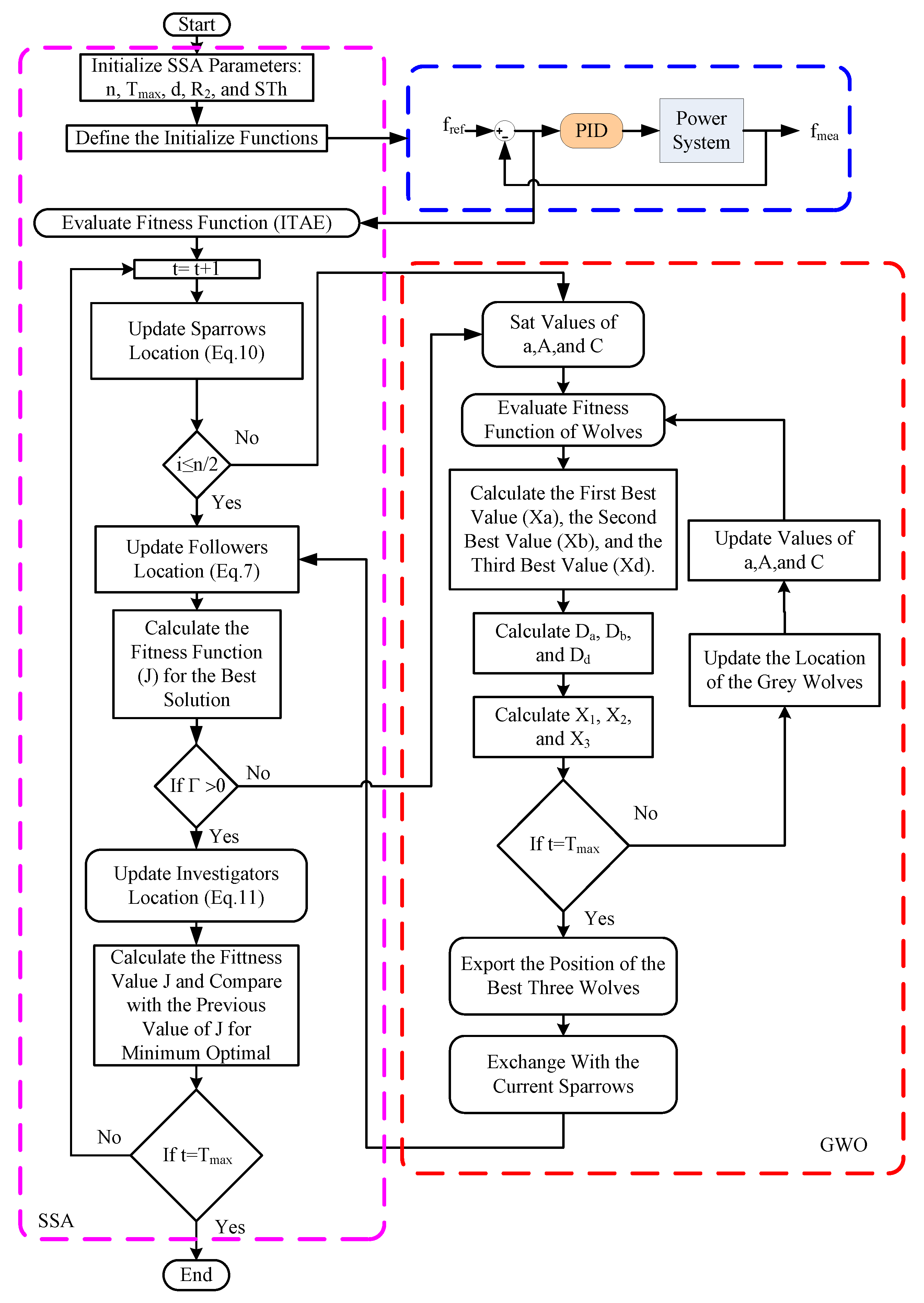
In this section, the proposed SSAGWO algorithm performance is first evaluated by comparing it with SSA and GWO algorithms in terms of statistical findings using five well-known benchmark functions from the literature. Furthermore, the proposed SSAGWO-tuned PID controller is analyzed for a two-area multi-source interconnected power system. The proposed SSAGWO optimized PID controller results are compared with SSA and GWO techniques. The obtained results for benchmark functions and various scenarios of the system model considered are discussed in detail in the following sections.

5.1. Validation of Benchmark Functions

Six classical benchmark functions with a wide range of characteristics are used to compare the proposed SSAGWO algorithm’s performance to that of GWO and SSA algorithms. The description of the benchmark functions used to verify the performance of various hybrid SSAGWO algorithms is shown in

Table 2. Benchmark functions.

Function Name		Type	Formula	Dimension (d)	Range
Sphere	F1	US	$f(x)={\displaystyle {\sum }_{i=1}^d{x}_i^2}$	30	[−100, 100]
Schwefel 2.21	F2	US	$f(x)={\max }_i\left\{\left|x_i\right|,1\le i\le d\right\}$	30	[−100, 100]
Schwefel 2.22	F3	UN	$f(x)={\displaystyle {\sum }_{i=1}^d\left|x_i\right|+{\displaystyle {\prod }_{i=1}^d\left|x_i\right|}}$	30	[−10, 10]
Rosenbrock	F4	UN	$f(x)={\displaystyle {\sum }_{i=1}^{d-1}\left[100{(x_{i+1}-x_i^2)}^2+{(x_i-1)}^2\right]}$	30	[−30, 30]
Rastrigin	F5	MS	$f(x)=10d+{\displaystyle {\sum }_{i=1}^d\left[x_i^d-10\cos (2\pi x_i)\right]}$	30	[−5.12, 5.12]
Ackley	F6	MN	$f(x)=-20\exp \left(-0.2\sqrt{\frac{1}{d}{\displaystyle {\sum }_{i=1}^d{x}_i^2}}\right)-\exp \left(\frac{1}{d}{\displaystyle {\sum }_{i=1}^d\cos 2\pi x_i}\right)+20+e$	30	[−32, 32]

. When referring to Table 2, the letter U indicates that the benchmark functions F1–F4 have a single global best and are unimodal. A function is said to be separable if and only if the letter S appears after the letter U in the notation. While if the letter N is written after the letter U, then the function is non-separable [3]. The exploitation ability of the optimization algorithm is investigated by the F1–F4 unimodal benchmark functions, as shown in Table 2, and they indicate that a robust local search capability is necessary for achieving good results. F5 and F6 are multimodal functions. These functions have multiple global bests and are used to investigate the optimization algorithm’s exploration ability. The multimodal functions are denoted with the letter M as shown in Table 2. The multimodal functions are also classified into separable and non-separable functions.

Table 3. Benchmark functions statistics.

Function	Index	SSAGWO	SSA	GWO
F1	Best	2.2339 × 10−31	2.7901 × 10−23	42.0302
	SD	3.3466 × 10−17	1.8513 × 10−19	10.11
	Mean	1.0642 × 10−17	6.6255 × 10−20	19.9949
	Min	0	2.4457 × 10−47	8.9247
F2	Best	5.1938 × 10−13	8.0550 × 10−12	22.7455
	SD	1.0443 × 10−10	2.2659 × 10−10	3.9943
	Mean	3.7025 × 10−11	7.8765 × 10−11	9.4191
	Min	1.6096 × 10−80	4.3857 × 10−55	5.3553
F3	Best	3.6567 × 10−13	1.6810 × 10−11	1.4005
	SD	4.9149 × 10−09	6.1537 × 10−10	0.3749
	Mean	1.7859 × 10−09	3.9256 × 10−10	1.3875
	Min	8.6574 × 10−58	1.2831 × 10−24	0.7203
F4	Best	2.8199 × 10−4	2.7812 × 10−2	548.2237
	SD	1.873 × 10−1	4.97 × 10−2	492.196
	Mean	1.113 × 10−1	5.28 × 10−2	963.3173
	Min	2 × 10−4	9.3 × 10−3	435.8798
F5	Best	0	0	76.6652
	SD	0	0	14.1344
	Mean	0	0	61.2244
	Min	0	0	36.401
F6	Best	8.8818 × 10−16	8.8818 × 10−16	2.4941
	SD	8.5631 × 10−11	7.1236 × 10−10	0.6564
	Mean	4.7806 × 10−11	3.0156 × 10−10	3.0160
	Min	8.8817 × 10−16	8.8817 × 10−16	1.3413

illustrates the statistical results of the optimization algorithm on the conventional benchmark functions. The results are compared based on the mean, minimum, and standard deviation of reaching the best values. The results were recorded for each algorithm 30 times running. Different benchmark functions are used to assess the algorithms GWO and SSA with SSAGWO by suggesting the algorithm population of 30 and 100 as a number of iterations. The results in Table 3 show that the SSAGWO has improved the exploration and exploitation ability compared with other optimization techniques. SSAGWO has mean, min, and standard deviation less than other algorithms.

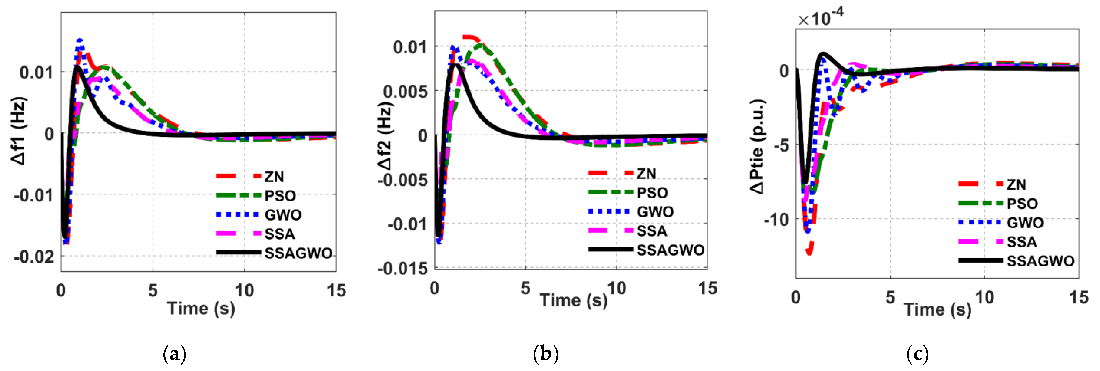
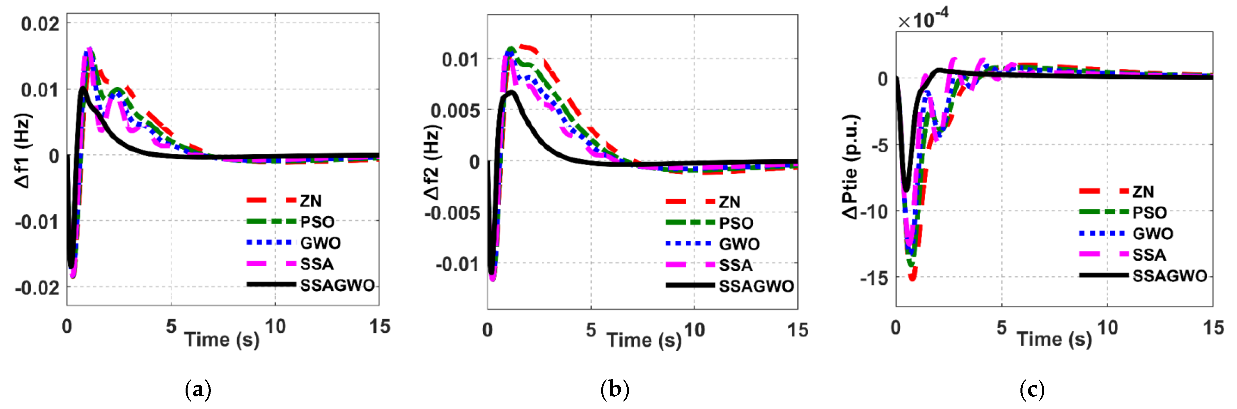
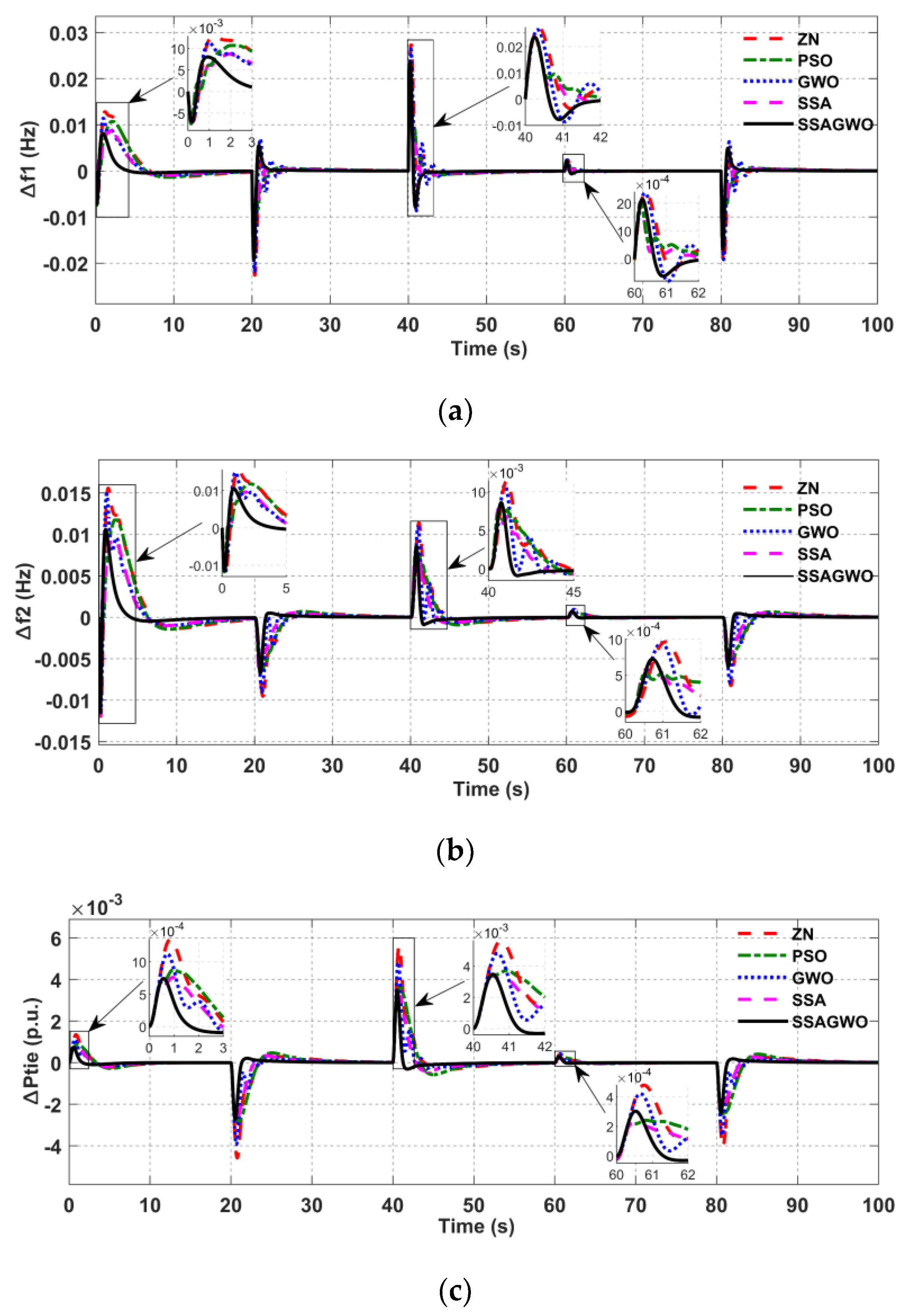
Three cases are presented to analyze the time domain response of the HPS as follows. Case I: In this case, area 1 is integrated with an SPV source, and area 2 is integrated with a WPG source. A step load change of 50 MW and 35 MW of the rated power system occurs in area 1 and area 2, respectively. Figure 8 shows the frequency deviation of four optimization techniques for tuning PID controller parameters (PSO, GWO, SSA, and SSAGWO) and the Z–N technique. It is clear from the figure that the ST of the proposed SSAGWO-optimized PID controller is much faster than the other optimization-tuned PID controller and Z–N-tuned PID controller.

Table 4. Frequency and power deviation in the tie-line power of case I.

Optimization Technique	Controller Effort	ST (s)	RT (s)	Undershoot	Steady-State Error
∆f1
Z–N	10.03 × 10−2	15.5747	1.3000 × 10−3	−1.85 × 10−2	−2.416 × 10−4
PSO	7.31 × 10−2	15.1049	8.9766 × 10−4	−1.69 × 10−2	−1.678 × 10−4
GWO	12.32 × 10−2	13.6758	7.3107 × 10−4	−1.82 × 10−2	−1.367 × 10−4
SSA	6.60 × 10−2	13.4111	5.9055 × 10−4	−1.69 × 10−2	−1.105 × 10−4
SSAGWO	5.95 × 10−2	3.8834	1.9259 × 10−4	−1.68 × 10−2	−3.608 × 10−5
∆f2
Z–N	7.14 × 10−2	16.7079	1.8 × 10−3	−1.23 × 10−2	−2.366 × 10−4
PSO	7.14 × 10−2	16.1989	1.3 × 10−3	−1.14 × 10−2	−1.643 × 10−4
GWO	6.24 × 10−2	15.1067	1.0 × 10−3	−1.22 × 10−2	−1.337 × 10−4
SSA	6.02 × 10−2	14.7612	8.2627 × 10−4	−1.14 × 10−2	−1.081 × 10−4
SSAGWO	5.18 × 10−2	9.9788	2.6857 × 10−4	−1.13 × 10−2	−3.521 × 10−5
∆Ptie
Z–N	6.6906 × 10−4	13.6500	2.957 × 10−1	−1.2 × 10−3	10.035 × 10−6
PSO	5.5430 × 10−4	14.0710	4.0090	−0.8 × 10−3	7.325 × 10−6
GWO	3.4650 × 10−4	11.5746	5.7 × 10−3	−1.1 × 10−3	6.509 × 10−6
SSA	5.3688 × 10−4	12.0433	2.87 × 10−2	−0.8 × 10−3	5.096 × 10−6
SSAGWO	1.1460 × 10−4	4.9285	2.0 × 10−3	−0.7 × 10−3	1.912 × 10−6

shows the results of the frequency deviation of area 1 and area 2 and the power deviation in the tie-line power. The ST of the proposed technique is improved by 75.06%, 74.29%, 71.60%, and 71.04% over Z–N, PSO, GWO, and SSA, respectively. Moreover, the RT of the frequency deviation of the proposed algorithm is less than other techniques by 85.18%, 78.54%, 73.65%, and 67.38%, respectively. In addition, the value of the undershoot of the frequency deviation is less than other techniques by 9.19%, 0.59%, 7.69%, and 0.59%, respectively. Furthermore, the results show that the steady-state error of the power system frequency when using the proposed SSAGWO is less by 85.06%, 78.49%, 73.60%, and 67.34%, respectively, than when using the other optimization techniques mentioned above. Furthermore, the steady-state values of the performance indices of the frequency deviation are improved by 30.43%, 70.45%, 39.50%, and 64.08% for the ISE, ITSE, IAE, and ITAE, respectively, compared with the best performance index of the optimization techniques presented in

Table 5. Steady-state indices in case I.

Performance Index	∆f1
	Z–N	PSO	GWO	SSA	SSAGWO
ITAE	22.81 × 10−2	20.45 × 10−2	14.77 × 10−2	13.860 × 10−2	4.978 × 10−2
IAE	5.787 × 10−2	4.785 × 10−2	4.296 × 10−2	3.625 × 10−2	2.193 × 10−2
ITSE	9.9 × 10−4	8.1 × 10−4	5 × 10−4	4.4 × 10−4	1.3 × 10−4
ISE	5 × 10−4	3.4 × 10−4	3.4 × 10−4	2.3 × 10−4	1.6 × 10−4
Performance Index	∆f2
	Z–N	PSO	GWO	SSA	SSAGWO
ITAE	22.22 × 10−2	20.070 × 10−2	14.4 × 10−2	13.64 × 10−2	4.845 × 10−2
IAE	5.236 × 10−2	4.425 × 10−2	3.816 × 10−2	3.322 × 10−2	1.862 × 10−2
ITSE	8.9 × 10−4	7.5 × 10−4	4.3 × 10−4	4 × 10−4	1 × 10−4
ISE	3.8 × 10−4	2.7 × 10−4	2.3 × 10−4	1.7 × 10−4	0.997 × 10−4

. Moreover, the proposed algorithm reduces the controller efforts by 40.67%, 18.60%, 51.70%, and 9.85% for Z–N, PSO, GWO, and SSA, respectively.

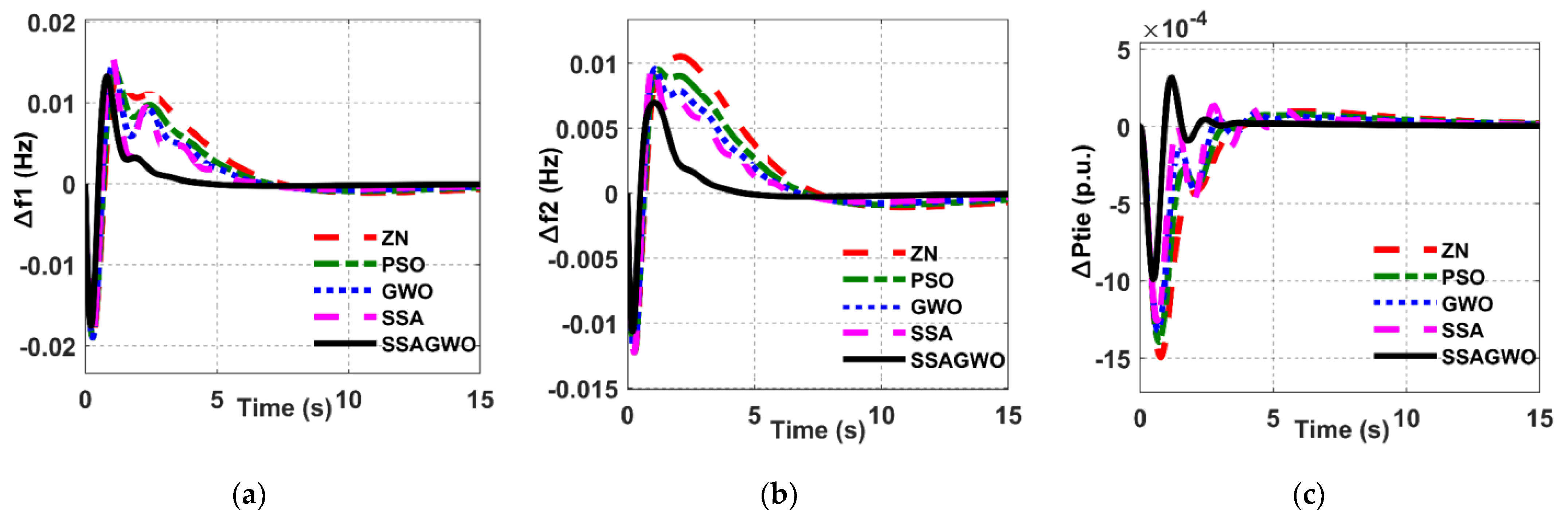
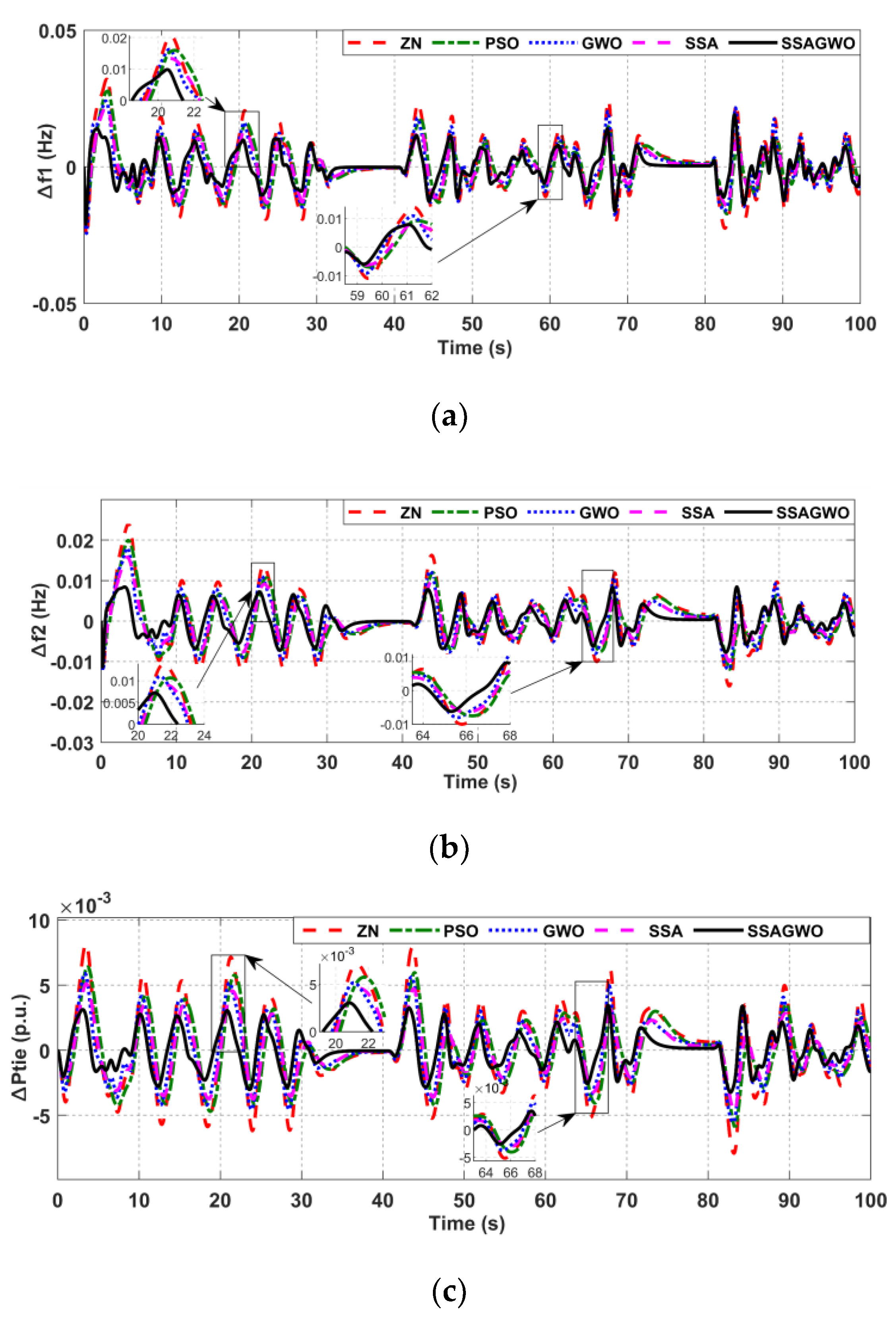
Case II: In this case, area 1 and area 2 are integrated with SPV resources. The step change in demand load applied in case II is similar to that of case I. Figure 9 shows the frequency deviation of the two areas and the power deviation in tie-line power for tuning PID parameters of the proposed SSAGWO compared with PSO, GWO, and SSA and the Z–N technique. Figure 9 demonstrates that the ST of the proposed SSAGWO-optimized PID controller is significantly less than that of the other optimization-tuned PID controllers and the Z–N-tuned PID controller. The results of the frequency deviation and tie-line power of case II are shown in

Table 6. Frequency and power deviation in the tie-line power of case II.

Optimization Technique	Controller Effort	ST (s)	RT (s)	Undershoot	Steady-State Error
∆f1
Z–N	14.71 × 10−2	15.5119	12.000 × 10−4	−1.84 × 10−2	−2.296 × 10−4
PSO	17.09 × 10−2	14.4838	8.8905 × 10−4	−1.84 × 10−2	−1.661 × 10−4
GWO	19.04 × 10−2	13.5912	6.9661 × 10−4	−1.83 × 10−2	−1.303 × 10−4
SSA	20.49 × 10−2	12.7962	5.7231 × 10−4	−1.83 × 10−2	−1.071 × 10−4
SSAGWO	8.060 × 10−2	3.73260	1.7247 × 10−4	−1.69 × 10−2	−3.231 × 10−5
∆f2
Z–N	8.96 × 10−2	16.7318	17.000 × 10−4	−1.16 × 10−2	−2.264 × 10−4
PSO	9.55 × 10−2	15.9302	13.000 × 10−4	−1.16 × 10−2	−1.637 × 10−4
GWO	10.32 × 10−2	15.1767	9.8148 × 10−4	−1.16 × 10−2	−1.283 × 10−4
SSA	11.09 × 10−2	14.4961	8.0590 × 10−4	−1.16 × 10−2	−1.054 × 10−4
SSAGWO	5.19 × 10−2	9.69000	2.4235 × 10−4	−1.09 × 10−2	−3.178 × 10−5
∆Ptie
Z–N	6.8776 × 10−4	12.0385	6.85 × 10−2	−1.5 × 10−3	6.506 × 10−6
PSO	6.9817 × 10−4	11.2029	81.85 × 10−2	−1.3 × 10−3	5.092 × 10−6
GWO	8.2955 × 10−4	10.5142	7.3 × 10−3	−1.3 × 10−3	4.183 × 10−6
SSA	17.000 × 10−4	9.7186	10.9 × 10−3	−1.2 × 10−3	3.547 × 10−6
SSAGWO	6.1746 × 10−4	6.4993	3.6 × 10−3	−0.8 × 10−3	1.167 × 10−6

. The ST of the proposed algorithm has been enhanced by 75.94%, 74.23%, 72.53%, and 70.83% compared with the ST of Z–N, PSO, GWO, and SSA, respectively. In addition, the RT of the frequency deviation of the proposed SSAGWO is less than other techniques by 85.63%, 80.60%, 75.24%, and 69.86%, respectively. Moreover, the peak undershoots value of the frequency deviation is less than other techniques by 8.15%, 8.15%, 7.65%, and 7.65%, respectively. Furthermore, the results shown in Table 6 depict that the steady-state error of the frequency deviation of the power system is less than other techniques by 85.93%, 80.54%, 75.20%, and 69.83%, respectively, when using the proposed SSAGWO to tune PID controller parameters.

The steady-state values of the ISE, ITSE, IAE, and ITAE all improve when using the proposed SSAGWO upon the best performance index of the optimization strategies shown in

Table 7. Steady-state indices in case II.

Performance Index	∆f1
	Z–N	PSO	GWO	SSA	SSAGWO
ITAE	22.71 × 10−2	17.88 × 10−2	14.71 × 10−2	12.45 × 10−2	4.658 × 10−2
IAE	5.845 × 10−2	4.97 × 10−2	4.356 × 10−2	3.899 × 10−2	2.069 × 10−2
ITSE	10.1 × 10−4	7 × 10−4	5.3 × 10−4	4.3 × 10−4	1.1 × 10−4
ISE	5.2 × 10−4	4.2 × 10−4	3.6 × 10−4	3.3 × 10−4	1.4 × 10−4
Performance Index	∆f2
	Z–N	PSO	GWO	SSA	SSAGWO
ITAE	21.72 × 10−2	17.07 × 10−2	14.03 × 10−2	11.91 × 10−2	4.393 × 10−2
IAE	5.146 × 10−2	4.32 × 10−2	3.747 × 10−2	3.33 × 10−2	1.679 × 10−2
ITSE	8.5 × 10−4	5.7 × 10−4	4.1 × 10−4	3.1 × 10−4	0.801 × 10−4
ISE	3.7 × 10−4	2.8 × 10−4	2.2 × 10−4	1.9 × 10−4	0.792 × 10−4

by 57.57%, 74.42%, 46.93%, and 62.58%, respectively. Moreover, the controller effort was reduced by 45.20%, 52.83%, 57.66%, and 60.66%, respectively, when using SSAGWO compared with other optimization techniques.

Case III: In this case, WTPG resources are integrated into both areas 1 and area 2. Figure 10 shows the frequency deviation and tie-line power of the HPS model. The figures show that the ST of the frequency deviation when using SSAGWO is less than the other optimization-tuned PID controller parameters mentioned above. The detailed results of this case are shown in Table 7. With the same sequence of comparing the proposed SSAGWO with other optimization techniques illustrated in case I and case II, the ST was improved by 75.40%, 73.66%, 71.88%, and 70.03%, respectively. In addition, the RT of the frequency deviation was reduced by 88.10%, 84.01%, 79.56%, and 75.15%, respectively. There is also a reduction in the peak undershoot value of the frequency deviation of 8.37%, 7.89%, 7.89%, and 7.41, respectively, compared to the other techniques.

Table 8. Frequency and power deviation in the tie-line power of case III.

Optimization Technique	Controller Effort	ST (s)	RT (s)	Undershoot	Steady-State Error
∆f1
Z–N	12.84 × 10−2	15.5405	13.000 × 10−4	−1.91 × 10−2	−2.5010 × 10−4
PSO	14.98 × 10−2	14.5127	9.6740 × 10−4	−1.90 × 10−2	−1.8080 × 10−4
GWO	17.32 × 10−2	13.5950	7.5658 × 10−4	−1.90 × 10−2	−1.4150 × 10−4
SSA	12.73 × 10−2	12.7563	6.2227 × 10−4	−1.89 × 10−2	−1.1640 × 10−4
SSAGWO	10.25 × 10−2	3.8229	1.5464 × 10−4	−1.75 × 10−2	−0.2898 × 10−4
∆f2
Z–N	8.55 × 10−2	16.7930	19 × 10−4	−1.22 × 10−2	−2.469 × 10−4
PSO	7.93 × 10−2	15.9452	14 × 10−4	−1.22 × 10−2	−1.783 × 10−4
GWO	8.88 × 10−2	15.1851	11 × 10−4	−1.22 × 10−2	−1.395 × 10−4
SSA	9.99 × 10−2	14.5028	8.7753 × 10−4	−1.22 × 10−2	−1.148 × 10−4
SSAGWO	6.48 × 10−2	8.8496	2.1741 × 10−4	−1.06 × 10−2	−0.285 × 10−4
∆Ptie
Z–N	7.2857 × 10−4	12.0973	58.7 × 10−3	−15 × 10−4	6.501 × 10−6
PSO	6.2357 × 10−4	11.2433	34.6 × 10−3	−14 × 10−4	5.083 × 10−6
GWO	8.4564 × 10−4	10.5482	7.9 × 10−3	−13 × 10−4	4.173 × 10−6
SSA	5.4 × 10−4	9.9408	9.1 × 10−3	−12 × 10−4	3.536 × 10−6
SSAGWO	1.7 × 10−4	3.8952	3.2793 × 10−3	−9 × 10−4	1.022 × 10−6

further demonstrates that using the proposed SSAGWO to tune PID controller parameters decreased the steady-state error of the frequency deviation of the power system by 88.41%, 83.97%, 79.52%, and 75.10%, respectively.

Compared to the best performance index of the optimization strategies presented in

Table 9. Steady-state indices in case III.

Performance Index	∆f1
	Z–N	PSO	GWO	SSA	SSAGWO
ITAE	23.42 × 10−2	18.45 × 10−2	15.17 × 10−2	12.87 × 10−2	3.995 × 10−2
IAE	5.882 × 10−2	5.01 × 10−2	4.401 × 10−2	3.947 × 10−2	1.978 × 10−2
ITSE	10.3 × 10−4	7.1 × 10−4	5.3 × 10−4	4.3 × 10−4	1.1 × 10−4
ISE	5.1 × 10−4	4.1 × 10−4	3.5 × 10−4	3.2 × 10−4	1.6 × 10−4
Performance Index	∆f2
	Z–N	PSO	GWO	SSA	SSAGWO
ITAE	22.43 × 10−2	17.65 × 10−2	14.51 × 10−2	12.29 × 10−2	3.749 × 10−2
IAE	5.18 × 10−2	4.357 × 10−2	3.787 × 10−2	3.366 × 10−2	1.524 × 10−2
ITSE	8.7 × 10−4	5.9 × 10−4	4.2 × 10−4	3.2 × 10−4	0.671 × 10−4
ISE	3.6 × 10−4	2.7 × 10−4	2.2 × 10−4	1.8 × 10−4	0.731 × 10−4

, the proposed SSAGWO improves the steady-state values of the ISE, ITSE, IAE, and ITAE by 50%, 74.42%, 49.88%, and 68.96%, respectively. In addition, SSAGWO reduced controller effort by 20.17%, 31.57%, 40.82%, and 19.48%, respectively, compared to other optimization methods.

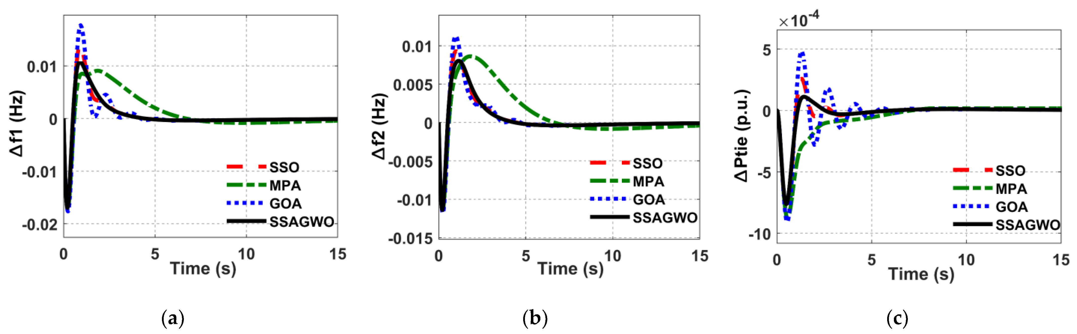
A comparison of the performance of the proposed hybrid SSAGWO optimization technique with the performance of the Grasshopper Optimization Algorithm (GOA) [17], Marine Predator Algorithm (MPA) [20], and Salp Swarm Optimization (SSO) [25] has been implemented in order to demonstrate the robustness of the suggested approach. Within the context of this discussion, case I has been utilized as a case study. Figure 11 depicts the dynamic response of the HPS model to the frequency deviation and the change in tie-line power. When compared with GOA, MPA, and SSO, the results demonstrate that the ST, overshoot, and oscillations of the frequency deviation, as well as the tie-line power, are improved when SSAGWO is utilized.

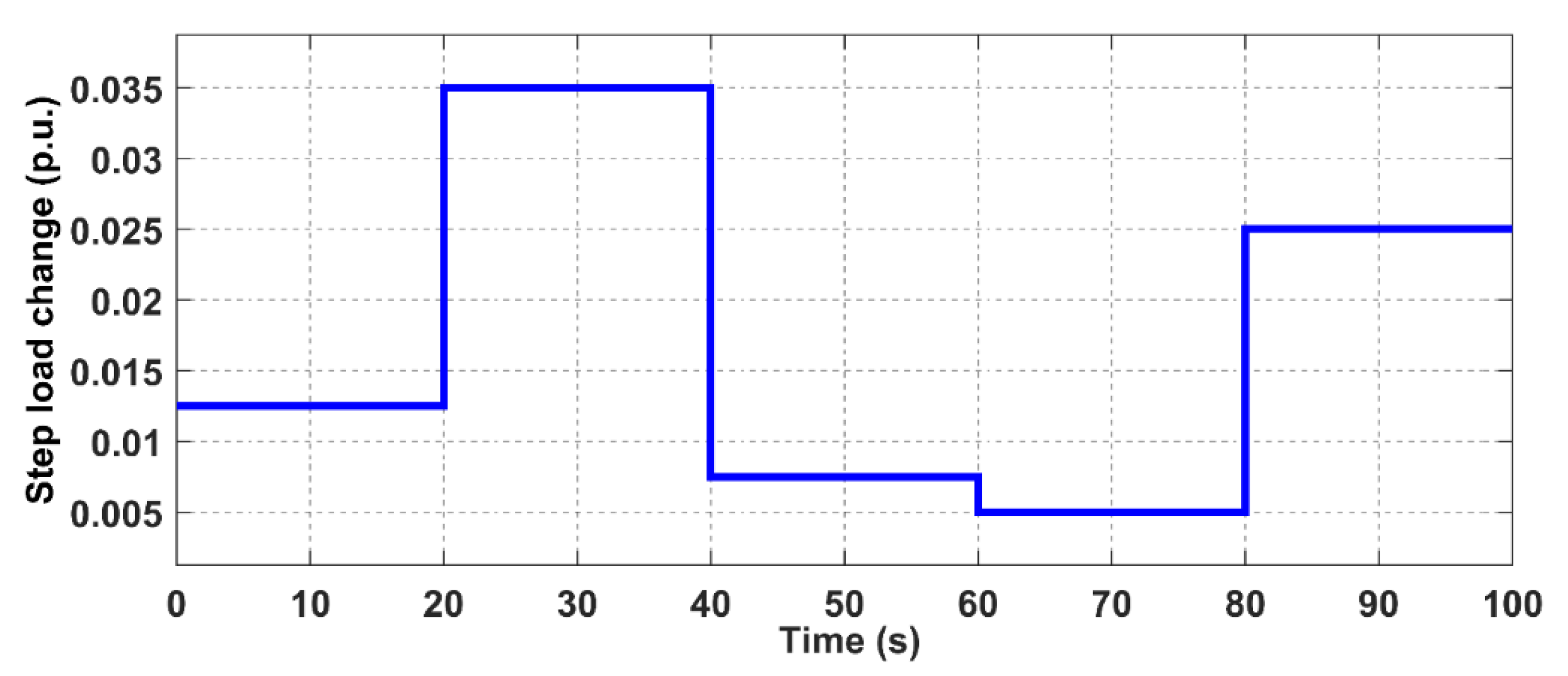
To study the effectiveness of the proposed algorithm, a random step change in load demand is applied in area 1, as shown in Figure 12. The frequency response of area 1, area 2, and tie-line power for this scenario are depicted in Figure 13. According to the findings, the proposed algorithm tunes the PID controller response more quickly for a sudden change in load than other optimization techniques do. Additionally, the power supplied by the tie-line changed in response to the changing load demands of the system while keeping a constant level of output despite these changes.

To further prove the robustness of the proposed technique, solar radiation data collected at Universiti Putra Malaysia, the output power from the SPV, is integrated with area 1 [3]. As shown in Figure 14, the solar irradiation values were measured from January through December 2014 for a total of 200 time-slots of 0.5 s. The multi-area power system in case I has been chosen to assess the dynamic response for real-time solar power fluctuations with all optimization techniques used in this study. The frequency deviation of area 1 and area 2 is shown in Figure 15 for this scenario. It can be deduced that the proffered SSAGWO algorithm-tuned PID controller shows a better and smoother response than other tuning methods, along with minimal undershoot, less ST, RT, steady-state error, and controller efforts.

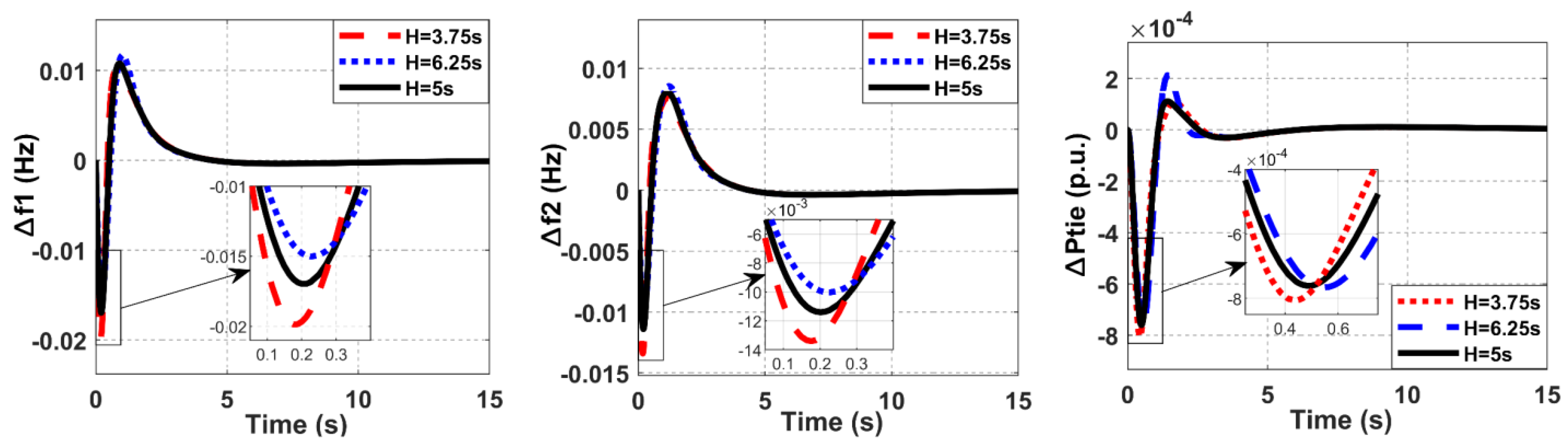
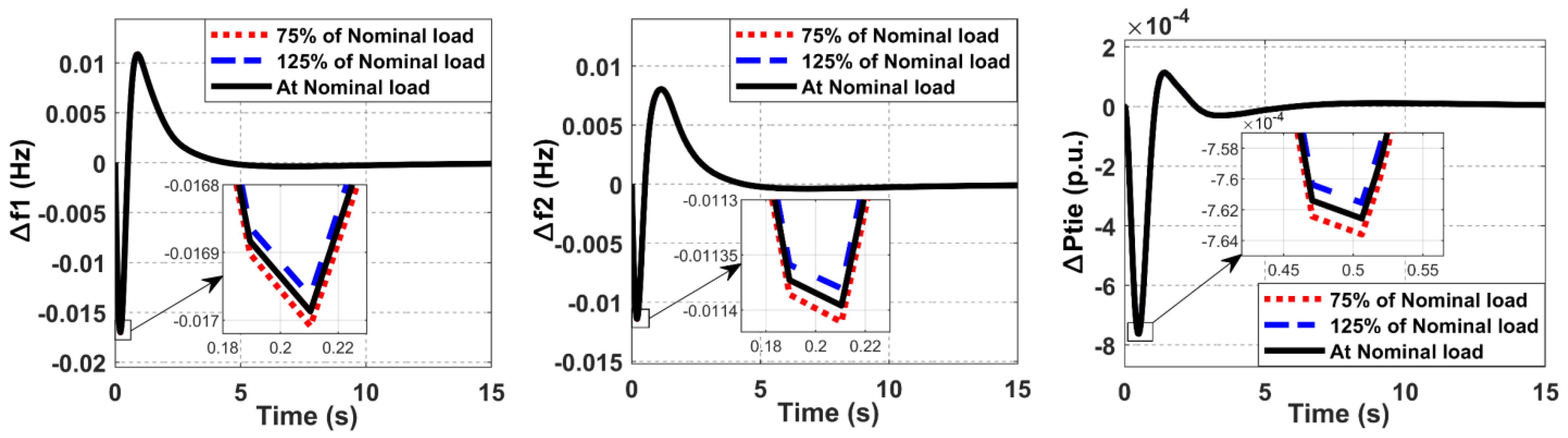
The sensitivity analysis of the proposed controller technique has been performed to prove the robustness of the controller parameters obtained under a variation of the inertia constant and change in the nominal loading of the power system.

The value of the inertia constant of the power system changed from 75% to 125% of its nominal value (H = 5), and the loading condition changed by ±25% compared with the nominal system loading (50% loading). The controller’s efficacy is demonstrated by using the value of the PID controller parameters under the nominal condition. Changing the inertia constant of the power system will affect the value of the time constant Tps. Likewise, the time constant of the power system block Tps and the gain constant Kps are affected by changes in load conditions. Figure 16 illustrates the dynamic response of the power system with variation in the inertia constant value. Figure 17 shows the dynamic response of the power system under change in the nominal loading. The result demonstrates a high tolerance for a wide range of changes in system parameters, as measured by the gain values obtained under nominal conditions. Because of this, one can draw the conclusion that the parameters do not need to be re-tuned even if there is a large amount of change in the system’s conditions and parameters.

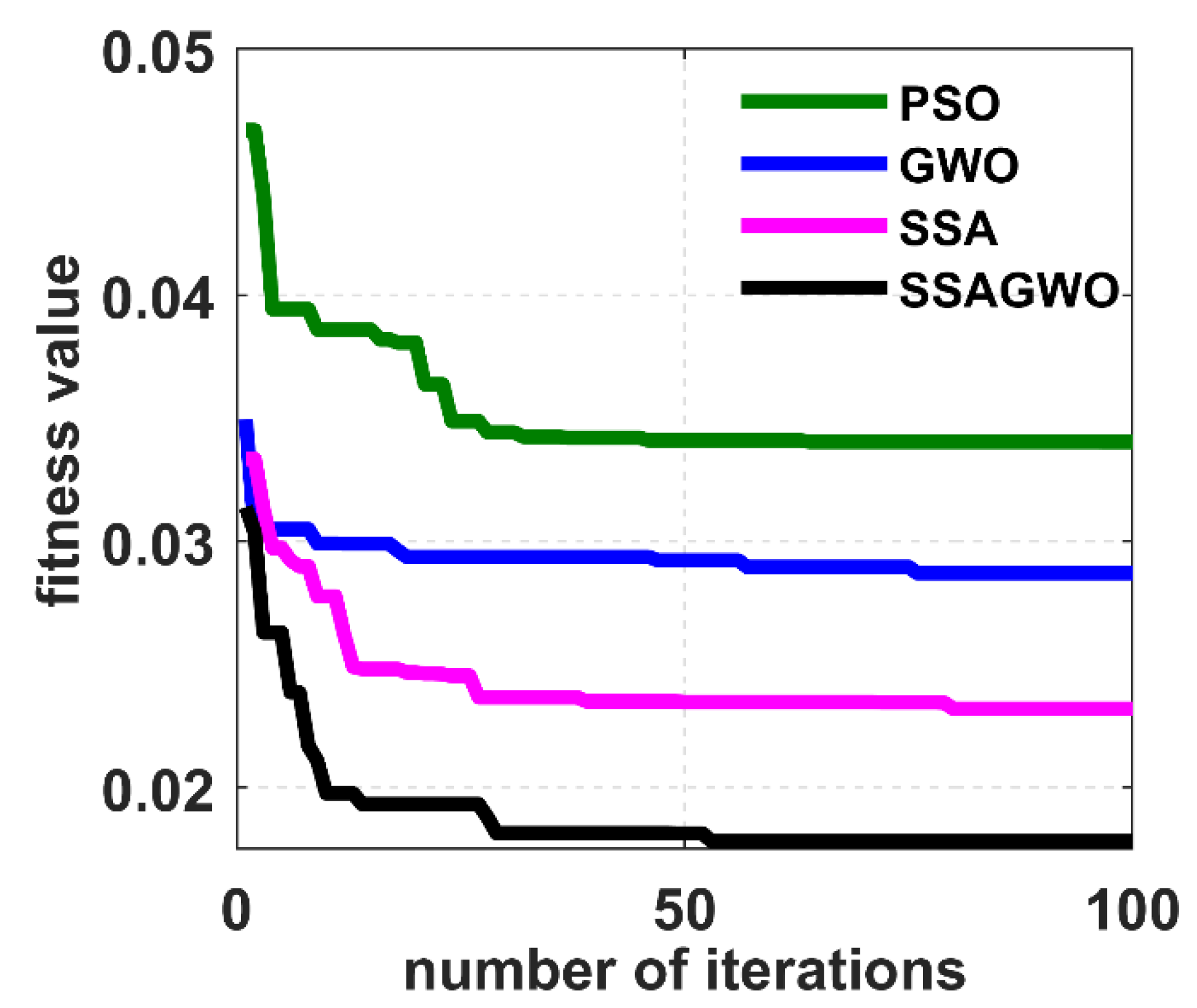
This section presents the convergence curves obtained by the proposed SSAGWO algorithm and other optimization algorithms. The convergence curve showing the minimum ITAE of ACE for the model is presented in Figure 18. The hybrid SSAGWO approach is shown to converge faster than other optimization methods, proving that the proposed SSAGWO has a better balance between exploration and exploitation than the standard GWO and SSA algorithms.

5.2. Stability Analysis

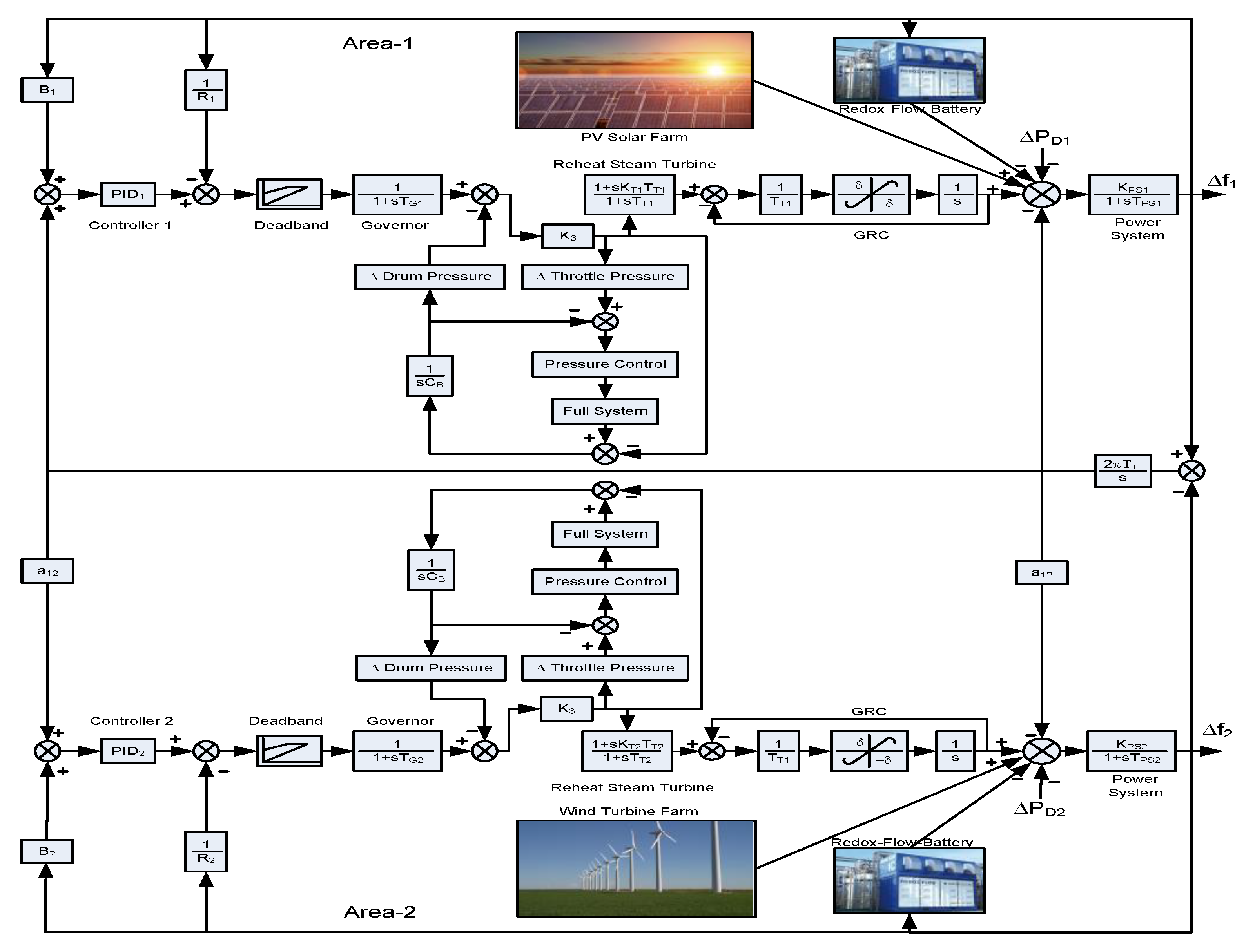
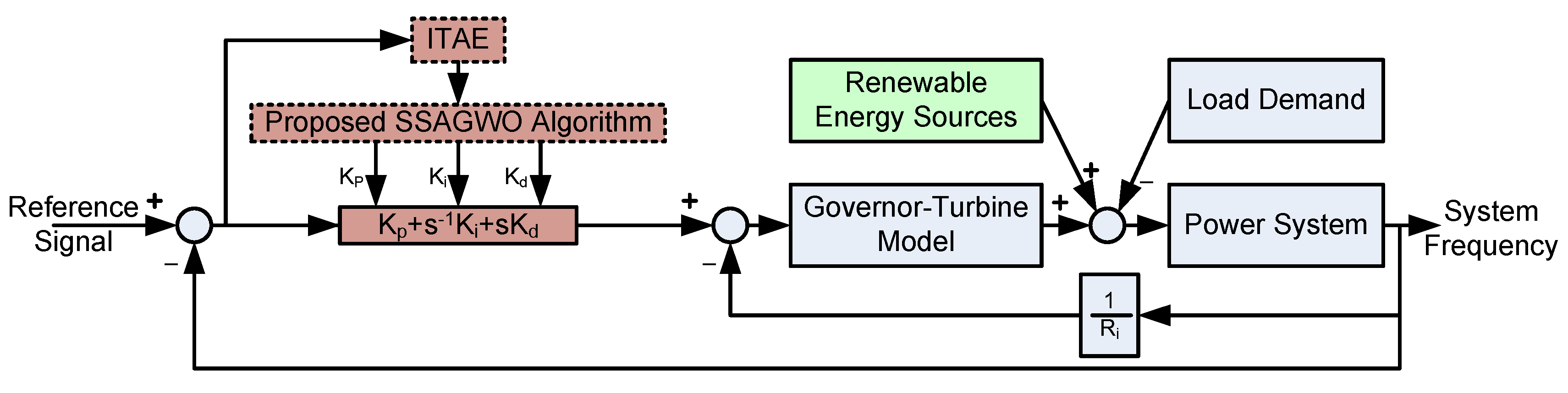
It is essential to take into consideration the effects of optimization techniques for PID tuning and validation of the stability analysis by calculating the state space of the system based on the Simulink model of the system. To assess the frequency stability of the power system and the HPS model optimized with SSAGWO-tuned PID controller parameters, two scenarios are considered. In scenario 1, Area I is considered as the input signal of the transfer function, while in scenario 2, Area II is considered as the input signal of the transfer function. The state-space equations with estimation of the Close Loop Transfer Function (CLTF) are illustrated as follows:

Let, ∆f_i = X₁, ∆P_Ti = X2, ∆T_T = X3, ∆P_tie,i = X5, ∆P_WT = X6, ∆P_PV = X7, and ∆P_RFB = X8

The vector form of the state variables of the proposed model is present in Equation (12):

$$X={\left[X_1,X_2,X_3,X_4,X_5,X_6,X_7,X_8\right]}^T$$

(12)

System parameters and their associated state variables are shown as below:

$$X={\left[\Delta f_i\Delta X_{1T}\Delta X_{1RE}\Delta P_{tie,i}\right]}^T$$

(13)

where

$$\Delta X_{1T}=\left[\Delta P_T\Delta T_T\Delta G_T\right]$$

(14)

$$\Delta X_{1RE}=\left[\Delta P_{WT}\Delta P_{PV}\Delta P_{RFB}\right]$$

(15)

The state-space equation of the HPS is illustrated as follows:

$$X_1^{•}=\frac{K_{pi}}{T_{pi}}\left[-X_1+X_2+X_3+X_4+X_5+X_6+X_7-X_8-\Delta P_{Di}\right]$$

(16)

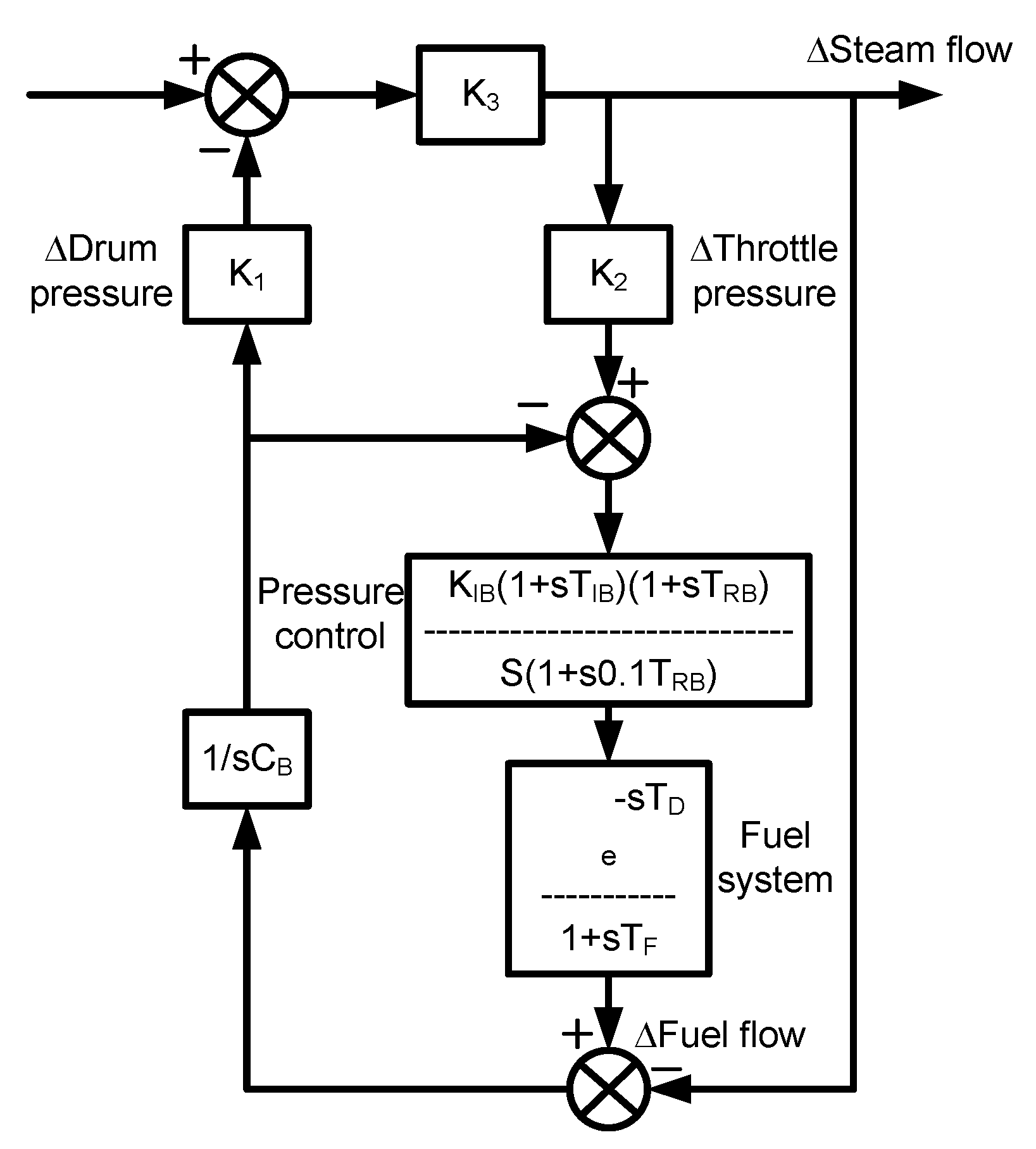
The state-space modeling of the reheat turbine generator is also derived in Equations (17)–(19):

$$X_2^{•}=-\frac{X_2}{T_{ti}}+\frac{X_3}{T_{ti}}$$

(17)

$$X_3^{•}=-\frac{X_3}{T_{ri}}+\left[\frac{1}{T_{ri}}-\frac{K_r}{T_{Gi}}\right]X_4+\frac{1}{T_{ri}}\Delta P_{ci}-\frac{X_1}{T_{ri}{R}_i}$$

(18)

$$X_4^{•}=-\frac{X_4}{T_{Gi}}+\frac{\Delta P_{ci}}{T_{Gi}}-\frac{1}{R_i{T}_{Gi}}{X}_1$$

(19)

In general, the state-space of the tie line power can be emulated as follows:

$$X_5^{•}=\Delta P_{tie,i}=2\pi \left[{\displaystyle \sum _{i=1,i\ne j}^n{T}_{ij}{X}_i}\right]$$

(20)

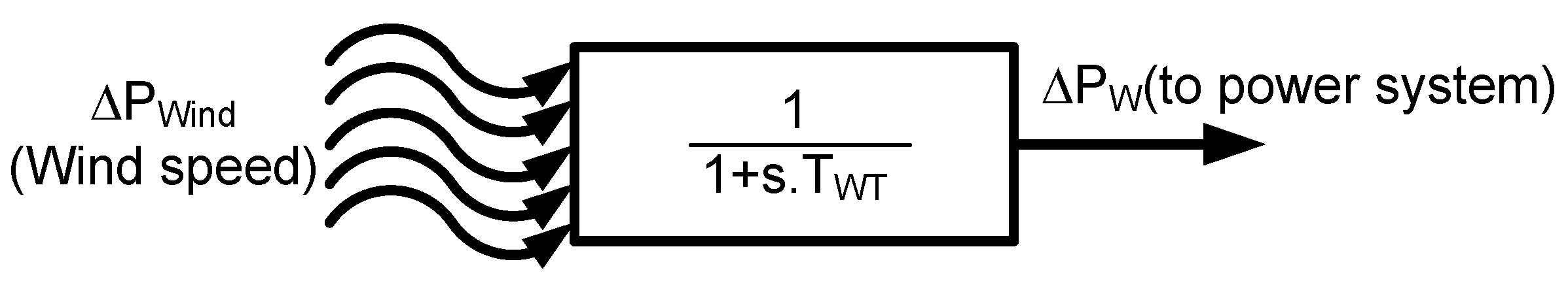
The wind turbine model in state space is given in Equation (21):

$$X_6^{•}=-\frac{X_6}{T_{WT}}+K_{WT}{P}_W$$

(21)

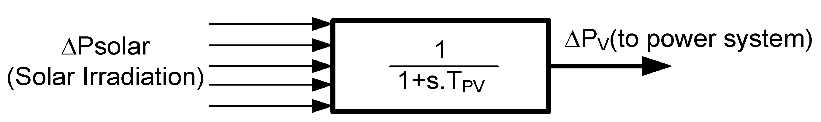
The PV model in state space is obtained in Equation (22):

$$X_7^{•}=-\frac{X_7}{T_{PV}}+K_{PV}{P}_V$$

(22)

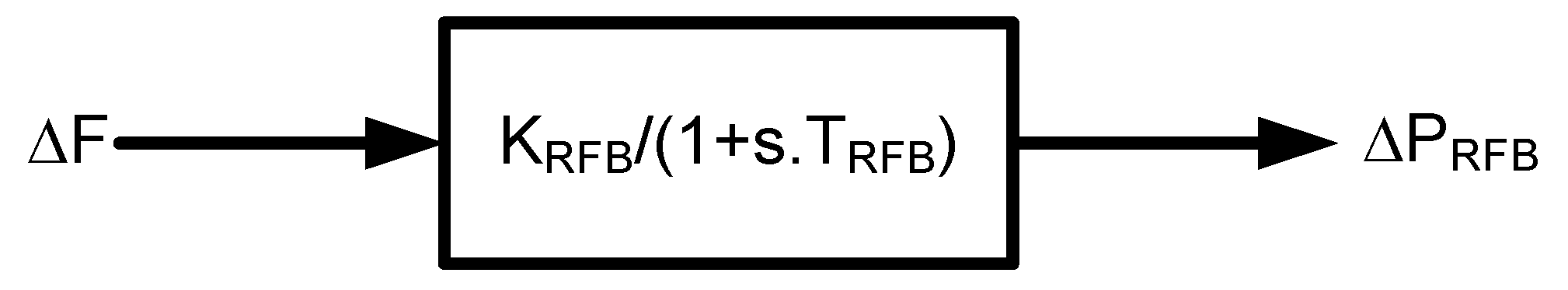
The state-space model of the RFB is shown below:

$$X_8^{•}=-\frac{X_8}{T_{RFB}}+K_{RFB}{P}_{RFB}$$

(23)

The general state-space representation is given below:

$$X^{•}=AX+Bu$$

(24)

where A is the state matrix, B is the input matrix, and C is the output matrix. According to the previous mathematical steps, A, B, and C can be calculated.

The control input can be presented as:

$$u={\left[\Delta P_{ci}\right]}^T$$

(25)

The definition of the output matrix of the proposed system is:

$$Y=CX$$

(26)

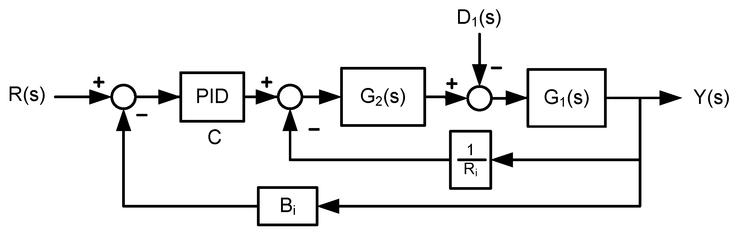
The closed loop control of the HPS shown in Figure 6, can be simplified as shows in Figure 19 in order to estimate the CLTF equation:

The derivation of the total response of the closed-loop transfer function of the interconnected power system was modeled with PID controller as the following:

$$R(s)G_2(s)G_1(s)C-B_{i}Y(s)C{G}_2(s)G_1(s)-Y(s)\frac{1}{R_i}{G}_2(s)G_1(s)-D_1(s)G_1(s)=Y(s)$$

(27)

$$Y(s)=\frac{R(s)G_1(s)G_2(s)C}{Z}-\frac{D_1(s)G_1(s)}{Z}$$

(28)

$$\therefore Y(s)=Y_{11}(s)+Y_{12}(s)$$

(29)

where

$$Z=1+B_{i}C{G}_1(s)G_2(s)+\frac{1}{R_i}{G}_1(s)G_2(s)$$

(30)

The change in load demand (∆P_D) is addressed for using the following expression for the CLTF of the system for the proposed controller:

$$\Delta f=\frac{-G_1}{1+G_1{G}_2\left[C{B}_i+\frac{1}{R}\right]}\Delta P_D$$

(31)

The CLTF can be applied to variations in tie-line power, as indicated by the definition of power variation:

$$\Delta f=\frac{C{G}_1{G}_2}{1+G_1{G}_2\left[C{B}_i+\frac{1}{R}\right]}\Delta P_{tie}$$

(32)

By using superposition theorem, the CLTF for the total variations of the frequency response can be defined as:

$$\Delta f=\frac{-G_1\Delta P_D+C{G}_1{G}_2\Delta P_{tie}}{1+G_1{G}_2\left[C{B}_i+\frac{1}{R}\right]}$$

(33)

By using the state-space analysis, the CLTF for the two scenarios (i.e., area 1 and area 2) can be presented as:

$$CLTF=\frac{num}{den}$$

(34)

Appendix B shows the state-space matrix, definition of the num, and den of the proposed power system model.

The proposed SSAGWO-tuned PID controller is of a higher order (11th), making stability analysis challenging. Therefore, the higher-order CLTF is reduced to a second-order transfer function using the Hankel matrix (HM) norm approximation method [48]. Detailed steps for reducing the higher-order transfer function are given below.

From the state-space in Appendix B, HM can be obtained. The general form of the HM can be presented as:

$$H_{nn}^0={\displaystyle \sum _{i=1}^n{\displaystyle \sum _{j=1}^n{(C{A}^{-n+1}B)}_{i,j}}}$$

(35)

The value of n = 13, therefore the HM is shown in Equation (35), which can be expressed as below:

$$H_{1313}^0={\displaystyle \sum _{i=1}^{13}{\displaystyle \sum _{j=1}^{13}{e}_{i,j}}}$$

(36)

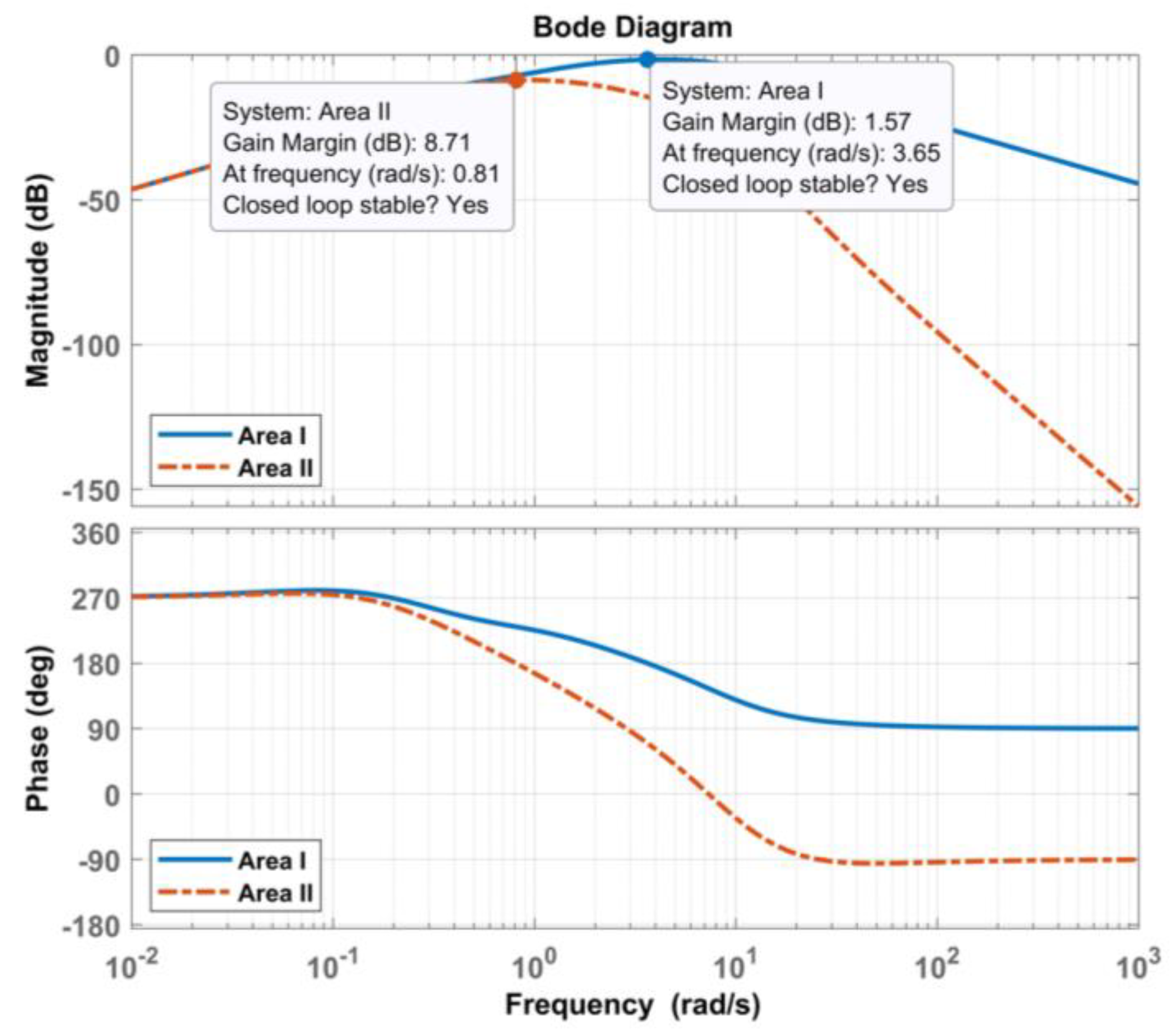
More detail about the HM technique to reduce the order of the CLTF of the proposed power system model has been given in [48]. To stabilize power generators, grid frequency should be controlled based on the droop characteristic that relates to the generator output [49]. Figure 20 depicts the frequency response of the Bode plot for the HPS model considering the two scenarios proposed in stability analysis, with a gain margin of 1.57 and 8.71 dB and a gain cross-over frequency of 3.65 and 0.81 (rad/s) for Area I and Area II, respectively. According to the Bode analysis response, the closed-loop system for the proposed SSAGWO optimized PID controller of the HPS network is stable.

6. Conclusions

In this manuscript, a hybrid SSAGWO algorithm is developed for optimal tuning of a PID controller for the load frequency control of multi-area interconnected power system. The proposed power system includes a high nonlinearity reheat steam station integrated with various RERs. The proposed SSAGWO optimization algorithm was utilized to enhance the parameters of the PID controller to minimize the frequency deviation in the presence of a PV system, wind turbine system generation, and load disturbance and to improve the robustness of the PID controller with SSAGWO contrary to the penetration of RERs and the effect of nonlinearities of the conventional plants of the HPS. Since the performance of the SSAGWO algorithm depends on minimizing the complexity of the fitness functions, the constraints and the boundaries of the proposed algorithm was modified by using the SSA algorithm and the GWO algorithm. This modified approach improves the dynamic performance of the LFC, while considering reduced-order of the entire transfer function for the sensitivity and stability analyses. In order to validate the dynamic performance and rigidity of the proposed optimization algorithm, a state-space model of the high-order close loop transfer function was computed in this work. Furthermore, the dynamic performance of the optimization algorithm was compared with PSO, GWO, SSA, GOA, MPA, and SSO. It is concluded that the SSAGWO achieved the best performance (i.e., settling time is 3.8834 s) in comparison with PSO, GWO and SSA; where the settling time values are 15.1049 s, 13.6758 s, and 13.4111 s, respectively.

References

1. Irudayaraj, A.X.R.; Wahab, N.I.A.; Premkumar, M.; Radzi, M.A.M.; Bin Sulaiman, N.; Veerasamy, V.; Farade, R.A.; Islam, M.Z. Renewable sources-based automatic load frequency control of interconnected systems using chaotic atom search optimization. Appl. Soft Comput. 2022, 119, 108574. [Google Scholar] [CrossRef]
2. Shouran, M.; Anayi, F.; Packianather, M. The bees algorithm tuned sliding mode control for load frequency control in two-area power system. Energies 2021, 14, 5701. [Google Scholar] [CrossRef]
3. Veerasamy, V.; Wahab, N.I.A.; Ramachandran, R.; Othman, M.L.; Hizam, H.; Kumar, J.S.; Irudayaraj, A.X.R. Design of single- and multi-loop self-adaptive PID controller using heuristic-based recurrent neural network for ALFC of hybrid power system Veerapandiyan. Expert Syst. Appl. 2022, 192, 116402. [Google Scholar] [CrossRef]
4. Mokhtar, M.; Marei, M.I.; Sameh, M.A.; Attia, M.A. An Adaptive Load Frequency Control for Power Systems with Renewable Energy Sources. Energies 2022, 15, 573. [Google Scholar] [CrossRef]
5. Arya, Y. AGC performance enrichment of multi-source hydrothermal gas power systems using new optimized FOFPID controller and redox flow batteries. Energy 2017, 127, 704–715. [Google Scholar] [CrossRef]
6. Huddar, A.P.; Kulkarni, P.S. Load frequency control of a multi-area power system using linear quadratic regulator. J. Inst. Eng. Electr. Eng. Div. 2009, 90, 69–76. [Google Scholar]
7. Wang, Z.; Liu, Y.; Yang, Z.; Yang, W. Load frequency control of multi-region interconnected power systems with wind power and electric vehicles based on sliding mode control. Energies 2021, 14, 2288. [Google Scholar] [CrossRef]
8. Mohamed, A.; Diab, A.A.Z.; Rezk, H.; Jin, T. A novel adaptive model predictive controller for load frequency control of power systems integrated with DFIG wind turbines. Neural Comput. Appl. 2020, 32, 7171–7181. [Google Scholar] [CrossRef]
9. Mohseni, N.A.; Bayati, N. Robust Multi-Objective H2/H∞ Load Frequency Control of Multi-Area Interconnected Power Systems Using TS Fuzzy Modeling by Considering Delay and Uncertainty. Energies 2022, 15, 5525. [Google Scholar] [CrossRef]
10. Soliman, M.S.; Belkhier, Y.; Ullah, N.; Achour, A.; Alharbi, Y.M.; Al Alahmadi, A.A.; Abeida, H.; Khraisat, Y.S.H. Supervisory energy management of a hybrid battery/PV/tidal/wind sources integrated in DC-microgrid energy storage system. Energy Rep. 2021, 7, 7728–7740. [Google Scholar] [CrossRef]
11. Al Alahmadi, A.A.; Belkhier, Y.; Ullah, N.; Abeida, H.; Soliman, M.S.; Khraisat, Y.S.H.; Alharbi, Y.M. Hybrid wind/PV/battery energy management-based intelligent non-integer control for smart DC-microgrid of smart university. IEEE Access 2021, 9, 98948–98961. [Google Scholar] [CrossRef]
12. Ramachandran, R.; Madasamy, B.; Veerasamy, V.; Saravanan, L. Load frequency control of a dynamic interconnected power system using generalised Hopfield neural network based self-adaptive PID controller. IET Gener. Transm. Distrib. 2018, 12, 5713–5722. [Google Scholar] [CrossRef]
13. Safari, A.; Babaei, F.; Farrokhifar, M. A load frequency control using a PSO-based ANN for micro-grids in the presence of electric vehicles. Int. J. Ambient. Energy 2021, 42, 688–700. [Google Scholar] [CrossRef]
14. Yesil, E. Interval type-2 fuzzy PID load frequency controller using Big Bang-Big Crunch optimization. Appl. Soft Comput. J. 2014, 15, 100–112. [Google Scholar] [CrossRef]
15. Veerasamy, V.; Wahab, N.I.A.; Ramachandran, R.; Vinayagam, A.; Othman, M.L.; Hizam, H.; Satheeshkumar, J. Automatic load frequency control of a multi-area dynamic interconnected power system using a hybrid PSO-GSA-Tuned PID controller. Sustainability 2019, 11, 6908. [Google Scholar] [CrossRef] [Green Version]
16. Guha, D.; Roy, P.K.; Banerjee, S. Load frequency control of interconnected power system using grey Wolf optimization. Swarm Evol. Comput. 2016, 27, 97–115. [Google Scholar] [CrossRef]
17. SNosratabadi, M.; Bornapour, M.; Gharaei, M.A. Grasshopper optimization algorithm for optimal load frequency control considering Predictive Functional Modified PID controller in restructured multi-resource multi-area power system with Redox Flow Battery units. Control Eng. Pract. 2018, 89, 204–227. [Google Scholar] [CrossRef]
18. Rai, A.; Das, D.K. Optimal PID Controller Design by Enhanced Class Topper Optimization Algorithm for Load Frequency Control of Interconnected Power Systems. Smart Sci. 2020, 8, 125–151. [Google Scholar] [CrossRef]
19. Paliwal, N.; Srivastava, L.; Pandit, M. Application of grey wolf optimization algorithm for load frequency control in multi-source single area power system. Evol. Intell. 2022, 15, 563–584. [Google Scholar] [CrossRef]
20. Sobhy, M.A.; Abdelaziz, A.Y.; Hasanien, H.M.; Ezzat, M. Marine predators algorithm for load frequency control of modern interconnected power systems including renewable energy sources and energy storage units. Ain Shams Eng. J. 2021, 12, 3843–3857. [Google Scholar] [CrossRef]
21. Gupta, D.K.; Jha, A.V.; Appasani, B.; Srinivasulu, A.; Bizon, N.; Thounthong, P. Load frequency control using hybrid intelligent optimization technique for multi-source power systems. Energies 2021, 14, 1581. [Google Scholar] [CrossRef]
22. Wang, X.; Wang, Y.; Liu, Y. Dynamic load frequency control for high-penetration wind power considering wind turbine fatigue load. Int. J. Electr. Power Energy Syst. 2020, 117, 105696. [Google Scholar] [CrossRef]
23. Yakout, A.H.; Attia, M.A.; Kotb, H. Marine Predator Algorithm based Cascaded PIDA Load Frequency Controller for Electric Power Systems with Wave Energy Conversion Systems. Alexandria Eng. J. 2021, 60, 4213–4222. [Google Scholar] [CrossRef]
24. Guha, D.; Roy, P.K.; Banerjee, S. Whale optimization algorithm applied to load frequency control of a mixed power system considering nonlinearities and PLL dynamics. Energy Syst. 2020, 11, 699–728. [Google Scholar] [CrossRef]
25. Hasanien, H.M.; El-Fergany, A.A. Salp swarm algorithm-based optimal load frequency control of hybrid renewable power systems with communication delay and excitation cross-coupling effect. Electr. Power Syst. Res. 2019, 176, 105938. [Google Scholar] [CrossRef]
26. Lu, P.; Ye, L.; Zhao, Y.; Dai, B.; Pei, M.; Tang, Y. Review of meta-heuristic algorithms for wind power prediction: Methodologies, applications and challenges. Appl. Energy 2021, 301, 117446. [Google Scholar] [CrossRef]
27. Almotairi, K.H.; Abualigah, L. Hybrid Reptile Search Algorithm and Remora Optimization Algorithm for Optimization Tasks and Data Clustering. Symmetry 2022, 14, 458. [Google Scholar] [CrossRef]
28. Sundararaju, N.; Vinayagam, A.; Veerasamy, V.; Subramaniam, G. A Chaotic Search-Based Hybrid Optimization Technique for Automatic Load Frequency Control of a Renewable Energy Integrated Power System. Sustainability 2022, 14, 5668. [Google Scholar] [CrossRef]
29. Pozna, C.; Precup, R.E.; Horvath, E.; Petriu, E.M. Hybrid Particle Filter-Particle Swarm Optimization Algorithm and Application to Fuzzy Controlled Servo Systems. IEEE Trans. Fuzzy Syst. 2022, 30, 4286–4297. [Google Scholar] [CrossRef]
30. Sureshkumar, V.; Balasubramaniam, S.; Ravi, V.; Arunachalam, A. A hybrid optimization algorithm-based feature selection for thyroid disease classifier with rough type-2 fuzzy support vector machine. Expert Syst. 2021, 39, 137–145. [Google Scholar] [CrossRef]
31. Gharehpasha, S.; Masdari, M.; Jafarian, A. Power efficient virtual machine placement in cloud data centers with a discrete and chaotic hybrid optimization algorithm. Cluster Comput. 2021, 24, 1293–1315. [Google Scholar] [CrossRef]
32. Dorigo, M.; Socha, K. Ant colony optimization. In Handbook of Approximation Algorithms and Metaheuristics; Chapman and Hall/CRC: New York, NY, USA, 2007; pp. 28–39. [Google Scholar] [CrossRef]
33. Zhao, W.; Zhang, Z.; Wang, L. Manta ray foraging optimization: An effective bio-inspired optimizer for engineering applications. Eng. Appl. Artif. Intell. 2018, 87, 103300. [Google Scholar] [CrossRef]
34. Castelli, M.; Manzoni, L.; Mariot, L.; Nobile, M.S.; Tangherloni, A. Salp Swarm Optimization: A critical review. Expert Syst. Appl. 2021, 189, 116029. [Google Scholar] [CrossRef]
35. Xue, J.; Shen, B. A novel swarm intelligence optimization approach: Sparrow search algorithm. Syst. Sci. Control Eng. 2020, 8, 22–34. [Google Scholar] [CrossRef]
36. Okwu, M.O.; Tartibu, L.K. Grey Wolf Optimizer. Stud. Comput. Intell. 2014, 927, 43–52. [Google Scholar] [CrossRef]
37. Yuan, J.; Zhao, Z.; Liu, Y.; He, B.; Wang, L.; Xie, B.; Gao, Y. DMPPT Control of Photovoltaic Microgrid Based on Improved Sparrow Search Algorithm. IEEE Access 2021, 9, 16623–16629. [Google Scholar] [CrossRef]
38. Irudayaraj, A.X.R.; Wahab, N.I.A.; Umamaheswari, M.G.; Radzi, M.A.M.; Bin Sulaiman, N.; Veerasamy, V.; Prasanna, S.C.; Ramachandran, R. A Matignon’s theorem based stability analysis of hybrid power system for automatic load frequency control using atom search optimized FOPID controller. IEEE Access 2020, 8, 168751–168772. [Google Scholar] [CrossRef]
39. Sahu, R.K.; Gorripotu, T.S.; Panda, S. A hybrid DE-PS algorithm for load frequency control under deregulated power system with UPFC and RFB. Ain Shams Eng. J. 2015, 6, 893–911. [Google Scholar] [CrossRef] [Green Version]
40. El-Ela, A.A.A.; El-Sehiemy, R.A.; Shaheen, A.M.; Diab, A.E.G. Enhanced coyote optimizer-based cascaded load frequency controllers in multi-area power systems with renewable. Neural Comput. Appl. 2021, 33, 8459–8477. [Google Scholar] [CrossRef]
41. Oshnoei, S.; Oshnoei, A.; Mosallanejad, A.; Haghjoo, F. Novel load frequency control scheme for an interconnected two-area power system including wind turbine generation and redox flow battery. Int. J. Electr. Power Energy Syst. 2021, 130, 107033. [Google Scholar] [CrossRef]
42. Dhandapani, L.; Abdulkareem, P.; Muthu, R. Two-area load frequency control with redox ow battery using intelligent algorithms in a restructured scenario. Turkish J. Electr. Eng. Comput. Sci. 2018, 26, 330–346. [Google Scholar] [CrossRef]
43. Sun, X.; Hu, C.; Lei, G.; Guo, Y.; Zhu, J. State feedback control for a PM hub motor based on gray Wolf optimization algorithm. IEEE Trans. Power Electron. 2020, 35, 1136–1146. [Google Scholar] [CrossRef]
44. Singh, N.; Singh, S.B. A Modified Mean Gray Wolf Optimization Approach for Benchmark and Biomedical Problems. Evol. Bioinform. 2017, 13, 1176934317729413. [Google Scholar] [CrossRef] [PubMed] [Green Version]
45. Xie, Q.; Guo, Z.; Liu, D.; Chen, Z.; Shen, Z.; Wang, X. Optimization of heliostat field distribution based on improved Gray Wolf optimization algorithm. Renew. Energy 2021, 176, 447–458. [Google Scholar] [CrossRef]
46. Liu, G.; Shu, C.; Liang, Z.; Peng, B.; Cheng, L. A modified sparrow search algorithm with application in 3D route planning for UAV. Sensors 2021, 21, 1224. [Google Scholar] [CrossRef]
47. Zhu, Y.; Yousefi, N. Optimal parameter identification of PEMFC stacks using Adaptive Sparrow Search Algorithm. Int. J. Hydrogen Energy 2021, 46, 9541–9552. [Google Scholar] [CrossRef]
48. Veerasamy, V.; Wahab, N.I.A.; Ramachandran, R.; Othman, M.L.; Hizam, H.; Irudayaraj, A.X.R.; Guerrero, J.M.; Kumar, J.S. A Hankel Matrix Based Reduced Order Model for Stability Analysis of Hybrid Power System Using PSO-GSA Optimized Cascade PI-PD Controller for Automatic Load Frequency Control. IEEE Access 2020, 8, 71422–71446. [Google Scholar] [CrossRef]
49. Idan, R.F.; Mahdi, A.J.; Wahhab, T.M.A. Optimized proportional-integral controller for a photovoltaic-virtual synchronous generator system. Int. J. Power Electron. Drive Syst. 2022, 13, 509–519. [Google Scholar] [CrossRef]
Figure 1. Transfer function model of the two-area power system.
Energies 16 01177 g001
Figure 2. Block diagram of the boiler dynamics configuration system.
Energies 16 01177 g002
Figure 3. Block diagram of PV dynamics system.
Energies 16 01177 g003
Figure 4. Block diagram of Wind turbine dynamics system.
Energies 16 01177 g004
Figure 5. Block diagram of Redox-Flow-Battery (RFB) model.
Energies 16 01177 g005
Figure 6. Close loop control system tuning.
Energies 16 01177 g006
Figure 7. Flow chart of the proposed hybrid SSAGWO algorithm technique.
Energies 16 01177 g007
Figure 8. The frequency deviation responses of the optimization techniques and conventional Ziegler–Nichols method for tuning PID controller parameters for case I: (a) The frequency deviation of area 1; (b) The frequency deviation of area 2; (c) The power deviation of the tie line.
Energies 16 01177 g008
Figure 9. The frequency deviation responses of the optimization techniques and conventional Ziegler–Nichols method for tuning PID controller parameters for case II: (a) The frequency deviation of area 1; (b) The frequency deviation of area 2; (c) The power deviation of the tie line.
Energies 16 01177 g009
Figure 10. The frequency deviation responses of the optimization techniques and conventional Ziegler–Nichols method for tuning PID controller parameters for case III: (a) The frequency deviation of area 1; (b) The frequency deviation of area 2; (c) The power deviation of the tie line.
Energies 16 01177 g010
Figure 11. The frequency deviation responses and change in tie line power of SSAGWO compared with GOA, MPA, and SSO for tuning PID controller parameters for case I: (a) The frequency deviation of area 1; (b) The frequency deviation of area 2; (c) The power deviation of the tie line.
Energies 16 01177 g011
Figure 12. Random change load.
Energies 16 01177 g012
Figure 13. Dynamic response of the multi-area power system at a random change load: (a) The frequency deviation of area 1; (b) The frequency deviation of area 2; (c) The power deviation of the tie line.
Energies 16 01177 g013
Figure 14. Realize solar input power.
Energies 16 01177 g014
Figure 15. Dynamic response comparison of the multi-area power system using various optimization techniques: (a) The frequency deviation of area 1; (b) The frequency deviation of area 2; (c) The power deviation of the tie line.
Energies 16 01177 g015
Figure 16. The dynamic response of the power system under different inertia constant (75% and 125% of the nominal value H = 5 s).
Energies 16 01177 g016
Figure 17. The dynamic response of the power system under different system loading (±25% of the nominal load).
Energies 16 01177 g017
Figure 18. Convergence curve of the algorithms.
Energies 16 01177 g018
Figure 19. The simplified closed loop control system for stability analysis.
Energies 16 01177 g019
Figure 20. Bode analysis of frequency stability.
Energies 16 01177 g020