Article

A Numerical Analysis of the Hybrid Nanofluid (Ag+TiO2+Water) Flow in the Presence of Heat and Radiation Fluxes

1
Department of Mathematical Sciences, University of Lakki Marwat, Lakki Marwat 28420, Khyber Pakhtunkhwa, Pakistan
2
Department of Mathematics and Sciences, Prince Sultan University, Riyadh 11586, Saudi Arabia
3
Mechanical Engineering Department, College of Engineering, Umm Al-Qura University, Makkah 24382, Saudi Arabia
4
Department of Industrial & Systems Engineering, College of Engineering, Princess Nourah bint Abdulrahman University, P. O. Box 84428, Riyadh 11671, Saudi Arabia
5
Department of Physics, Kohat University of Science & Technology, Kohat 26000, Khyber Pakhtunkhwa, Pakistan
6
Department of Mathematics and Statistics, Hazara University, Mansehra 21120, Khyber Pakhtunkhwa, Pakistan
*
Author to whom correspondence should be addressed.
Submission received: 14 December 2022 / Revised: 11 January 2023 / Accepted: 14 January 2023 / Published: 22 January 2023

Abstract

:
The hydrothermal characteristics of (Ag+TiO 2 +H 2 O) hybrid nanofluid three dimensional flow between two vertical plates, in which the right permeable plate stretches as well as rotates, are investigated by employing varying magnetic, heat and radiation fluxes. The motion is governed by coupled PDEs (nonlinear) obeying suitable boundary conditions. The PDEs coupled system is transformed to a coupled set of nonlinear ODEs employing appropriate similarity transformation relations. The resultant equations are numerically solved through the bv4c solver. The impact of the changing strength of associated parameters on the flow is investigated graphically and through tables. It has been found that the velocity gradient and velocity initially increase and then decrease with increasing Grashof number values in both the suction and injection cases. The enhancing magnetic field first augments and then lowers the velocity gradient in the presence of radiation source of maximum strength. The increasing strength of injection parameter drops the velocity. The temperature distribution in the fluid increases with the increasing Eckert number, radiation flux and heat strength and nanomaterial concentration, and depreciates with the enhancing injection parameter values and Prandtl number. The C f x increases with a higher magnetic field magnitude and nanomaterial concentration, and declines with an increasing Grashof number. The results obtained are compared with the available literature in the form of tables.

1. Introduction

The study of energy transfer finds importance and applications in almost every field of science and technology. The transfer of thermal energy takes place due to either conduction, convection, or radiation, or a combination of these processes. In conduction, heat energy transfers due to direct contact, while in convection, the accumulative motion of fluid particles causes heat energy transfer. Thermal energy also transfers from one point to another point in the form of electromagnetic waves; this mode is termed radiation. The fluids which are employed ordinarily for thermal energy transport through convection mode are ethylene glycol, ethylene, water, etc. Such fluids have poor heat energy transport capability. The heat energy transfer capability of these fluids may be augmented by mixing particles of suitable nature and size. If the dimension of these mixing particles are of nanometer range and of metallic nature, then their mixing with the usual fluids can enhance the radiant energy transport capacity very significantly [1,2]. The fluid which is formed by merging the fluids with nanomaterials are known as nanofluid. This fascinating idea was initially presented by Choi [3]. The different physical and thermal characteristics (such as heat capacity, thermal conduction, and viscosity) of nanofluids depend highly on the associated nanomaterial’s attributes, such as size, nature, and temperature, and concentration of the ordinary fluids. Researchers globally have examined heat energy transport capacity under a variety of restrictions to model the dynamics of these innovative fluids [4,5]. Nanofluids have extensively been used in solar energy systems [6,7], heat energy exchangers [8,9,10], freezing phenomena [11], and energy transfer due to electromagnetic waves [12,13,14]. Mebarek-Oudina [15] examined the thermal energy properties of nanofluids by employing different types of usual fluids. Muhammad et al. [16] numerically modeled the magneto-hydro-dynamic (MHD) flow of nanofluid by considering the motile microorganisms and slip effects. Nahid [17] studied nonlinear equations by using perturbation methods. The Darcy–Forchheimer flow from a curved body of a nanofluid was studied by Sajjad et al. [18] analytically. Nanofluid motion through variable-induced flux via a model of second-grade fluid was studied by Ambreen et al. [19]. Qasim et al. [20] analyzed ferrofluid flow by considering the flux of heat and velocity slip effects though a stretching cylinder. Afridi and Qasim [21] studied numerically the entropy generation inside the dissipative 3 D flow. Qasim [22] studied the heat and mass transfer analysis of Jeffrey fluid though a stretching surface. He reported that the thermal boundary layer declines with the larger values of the wall temperature and sink parameter. A recent study of nanofluids was undertaken in references [23,24,25,26,27].
In recent times, enormous interest has developed in investigating the heat energy transfer attributes of hybrid nanofluids (HNs). These fluids are formed by intermixing nanoparticles of different kinds in host fluids. Hybrid nanofluids posses improved and distinct thermophysical properties in comparison with ordinary nanofluids. To date, different types of hybrid nanoliquids have been developed [28,29,30]. The research work shows that HNs are more prominent and versatile in comparison to single-component nanofluids. Suresh et al. [31] analyzed the thermal properties of an HN obtained by merging alumina and copper nanoparticles with the host fluid, employing a two-step technique. Chamkha et al. [32] undertook a study of the distinct characteristics of time-dependent conjugate migration of (Cu+Al 2 O 3 +H 2 O) an HN using a triangular enclosure. They claimed a sufficient increase in the HN convective transport of heat energy. Momin [33] experimentally analyzed the HN laminar and mixed convective flow through an inclined tube. Qadeer et al. [34] studied numerically the entropy optimization for a 3 D HN squeezing flow. Their results show that with larger values of the magnetic parameter and Eckert number, both the temperature and entropy produced are boosted. The friction parameter and thermal energy transfer properties of (MWCNT+Fe 3 O 4 +H 2 O) HN were studied by Sundar et al. [35]. The energy transport rate was investigated by Ghachem et al. [36] by employing a hybrid nanofluid using a heat exchanger. Lund et al. [37] examined the impact of viscosity on (Cu+Al 2 O 3 +H 2 O) HN migration over a squeezing surface by performing a stability analysis. Suresh et al. [38] studied (copper + alumina) nano-powders for the efficient operation of thermal energy system. They used host fluid as water. Afridi et al. [39] analyzed the Cu+Al 2 O 3 +H 2 O and Cu+Al 2 O 3 +kerosene oil hybrid nanofluids (HN) numerically. The impact of various parameters such as Eckert number on the state variables was analyzed, and the study further suggested that the thermal boundary layer thickness is higher compared to conventional fluids. Usman et al. [40] studied the Cu+Al 2 O 3 +H 2 O HN migration from a perforated enclosure, considering the impact of variable thermal conduction rate and a source of radiation, using the least squares method (LSM). A numerical study of the impacts due to (MWCNT+Fe 3 O 4 +H 2 O) HN motion through a corrugated channel with distinct cooling (heating) sections was undertaken by Mohebbi et al. [41] applying LSM. Minna et al. [42] presented a thorough review by discussing the development of HNs and their applications.
This manuscript is concerned with the radiant energy transport properties of (Ag+TiO 2 +H 2 O) HN flow between vertical plates, considering the effects of changing magnetic flux, heat energy and radiation sources. The right side plate is permeable, rotates with Ω (angular velocity), and stretches with U w . The investigation may find enough importance in the system for the transfer of energy using HN. The article is arranged as: The flow of the chosen HN is assumed between plates in which one of the plates (the right one) is rotatory, permeable and stretching in the presence of variable magnetic field, radiation and the heat source. The problem is mathematically structured by PDEs which are nonlinear and coupled in Section 2. A simple and soluble system of ODEs is then obtained via similarity relations in Section 3. The resultant ODEs are numerically tackled through bv4c in Section 4. The results are discussed through graphs and tables in Section 5. A summary points of the investigations is presented in Section 6.

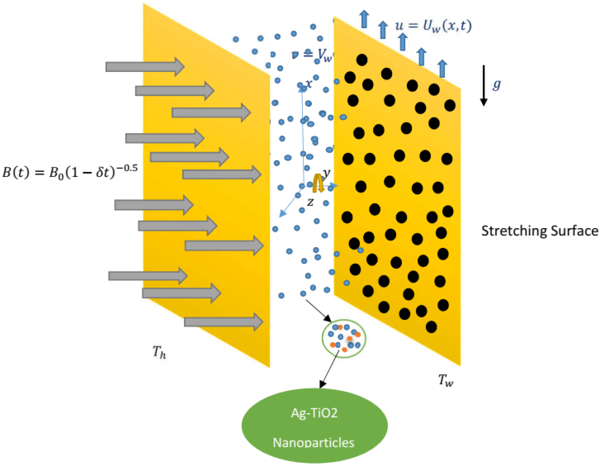
2. Problem Formulation

Consider the chosen HN (Ag+TiO 2 +H 2 O) motion through two vertical plates in the state of magnetic flux, thermal energy source and nonlinear radiation flux. The right plate of the configuration is rotating with Ω around the y-axis, and is permeable. Furthermore, the right wall is stretching with velocity U w = χ ( 1 δ t ) 1 , with χ t < 1 ; here, δ and χ are constants. The no-slip condition is not taken into consideration due to thermal equilibrium between the base fluid and nanoparticles. A time-varying magnetic field ( B ( t ) = B 0 ( 1 δ t ) 0.5 ) is acting orthogonal to the fluid motion. The flow is assumed to be incompressible and the pressure due to the fluid migration and the rotating wall is neglected. The velocity near the wall is V w and corresponds to the injection/suction case for positive and negative values of the parameter, respectively, as shown in Figure 1 [43,44]. Various impacts, for example, viscous dissipation and Coriolis effect, are taken into consideration in the fluid motion.
Keeping in view these assumptions, the given problem can be modeled as [44,45,46]:
u x + v y + w z = 0 ,
ρ h n f u t + u u x + v u y + 2 Ω w = p x + μ h n f u x x + u y y σ h n f B 2 ( t ) ( 1 + m 2 ) u + g ( ρ β ) h n f ( T T w ) ν K u ,
ρ h n f v t + u v x + v v y = p y + μ h n f v x x + v y y ,
ρ h n f w t + u w x + v w y 2 Ω w = μ h n f w x x + w y y σ h n f B 2 ( t ) ( 1 + m 2 ) w ν K w ,
( ρ C p ) h n f T t + u T x + v T y + w T z = k h n f T x x + T y y + T z z + μ h n f 2 u x 2 + v y 2 + w z 2 + v x 2 + v z 2 + w x + u z 2 + Q s ( T T w ) q y r .
Here, ρ h n f , σ h n f , k h n f , μ h n f , and ( ρ C p ) h n f are the HN properties, B ( t ) is the magnetic field, and Q s is the radiant energy source. The flux q r of radiation is expressed as [43]:
q r y = 16 σ s T 3 3 k 1 2 T y 2 ,
here, k 1 ( σ s ) denotes the absorption coefficient (Stefan constant). Equations (1) to (5) satisfy the following B.Cs [46]:
u = U w , v = V w , w = 0 , T = T h , at y = 0 , u 0 , v s . 0 , w 0 , T T w , at y h .
where, V w = ν χ 1 δ t 0.5 f ( η ) designates the flow at y = 0 and corresponds to injection (suction/injection) subjected to V w > 0 ( V w < 0 ). The properties of the nanoparticles and the base fluid are given in Table 1, where as, different parameters of the HN components are given in Table 2.

3. Similarity Transformations

Equations (1) to (7) are transformed by employing the similarity transformations [45]:
u = χ x ( 1 δ t ) f ( η ) , v = χ ν 1 δ t 0.5 f ( η ) , θ = T T w T h T w , w = χ x 1 δ t 0.5 g ( η ) , η = y χ ν ( 1 δ t ) 0.5 .
Using (8), we have:
f R ϵ 1 ϵ 2 ( f f f f ) 2 K r ϵ 1 ϵ 2 g ϵ 5 M ϵ 2 ( 1 + m 2 ) f R e ϵ 1 ϵ 2 G r β θ A 0 ( η 2 f + f ) + γ 0 f = 0 ,
g R ϵ 1 ϵ 2 ( f g f g ) + 2 K r ϵ 1 ϵ 2 f ϵ 5 M ϵ 2 ( 1 + m 2 ) g + A 0 ( η 2 g + g ) γ 0 g = 0 ,
θ + P r ϵ 2 ϵ 3 ϵ 1 ϵ 4 R e ϵ 1 ϵ 2 f θ + E c ϵ 1 ϵ 3 ( 4 f 2 + g 2 ) + ϵ 1 ϵ 2 ϵ 3 R e Q θ / ( 1 + 4 R d 3 ϵ 4 ) A 0 η 2 θ = 0 .
The boundary conditions transform as:
f ( η ) = S , f ( η ) = 1 , g ( η ) = 0 , θ ( η ) = 1 : η = 0 , f ( η ) 0 , g ( η ) 0 , f ( η ) 0 , θ ( η ) 0 : η 1 .
Here, ϵ 1 = ρ h n f ρ f , ϵ 2 = μ e f f μ f , ϵ 3 = ( ρ C P ) h n f ( ρ C p ) f , ϵ 4 = k K f , ϵ 5 = σ h n f σ f , and A 0 = δ χ are constants, γ 0 = ν f χ K is the porosity parameter, G r = g β f ( T h T w ) χ 2 x is the Grashof number, β = β h n f β f is the expansion (thermal) coefficient, Q = Q 0 χ ( ρ C p ) f ( R d = 16 σ s T h 3 3 k k s ) is the source or sink of heat (radiation), M = σ f B 0 2 h 2 ρ f ν f is the magnetic parameter, k r = Ω h 2 ν f is the rotational parameter, P r = μ ( ρ C p ) f ρ f k f is the Prandtl number, E c = ρ f a 2 h 2 ( ρ C p ) f ( T w T h ) Eckert number, and R e = χ h 2 ν f is the Reynolds number.

4. Numerical Solution

In the fluid flow problems, and especially in boundary layer equations, the homotopy analysis method, Kellerbox method, Laplace transform, and shooting technique etc. are widely employed for the the model equations solution. A brief survey on these types of equations is presented by Verma and Mondal [48], by using the Casson fluid model. Furthermore, Rai and Mondal [49] present a more detailed report on spectral methods. Oyelakin et al. [50] present the Casson fluid problem by considering the quasi-linearization technique with multi and bi-variations in the domain. In the literature, a bv4c Matlab solver is very commonly used for solving nonlinear ODEs, especially in fluid mechanics. The results obtained through bv4c as a special case give similar results to those obtained through semi-analytical and numerical approaches. To use this technique, we first transform the system of Equations (9)–(12) into the first order initial value problem (IVP). The transformed system is then solved by applying bv4c. For this, assume that
f = y 1 , f = y 2 , f = y 3 , f = y 4 , g = y 5 , g = y 6 , θ = y 7 , θ = y 8
y 1 = f , y 2 = y 3 , y 3 = y 4 , y 4 = 1 + R ϵ 1 ϵ 2 y 1 1 [ R ϵ 1 ϵ 2 y 2 y 4 + 2 k r y 6 + ϵ 5 M ϵ 2 y 3 + R ϵ 1 ϵ 2 G r β * y 8 + A 0 η 2 y 3 + y 2 + M 2 1 + m 2 ( y 2 + m y 5 ) γ 0 y 3 ] y 5 = g , y 5 = y 6 , y 6 = R ϵ 1 ϵ 2 y 2 y 5 y 1 y 6 2 k r ϵ 1 ϵ 2 y 2 + ϵ 5 M ϵ 2 y 5 A 0 η 2 y 6 + y 5 + M 2 1 + m 2 ( m y 2 y 5 ) + γ 0 y 5 y 7 = θ , y 7 = y 8 , y 8 = P r ϵ 2 ϵ 3 ϵ 1 ϵ 4 [ R ϵ 1 ϵ 2 y 1 y 7 + E c ϵ 1 ϵ 3 ( 4 y 2 2 + y 5 2 ) + ϵ 1 ϵ 2 ϵ 3 R Q y 7 ] 1 + 4 R d 3 ϵ 4 1 + A 0 η 2 y 8 ,
and BCs are:
y 1 ( 0 ) = S , y 2 ( 0 ) = 1 , y 5 ( 0 ) = 0 , y 7 ( 0 ) = 1 , y 1 ( 1 ) = 0 , y 2 ( 1 ) = 0 , y 5 ( 1 ) = 0 , y 7 ( 1 ) = 0 .
The system of Equations (13)–(15) is now solved by using bv4c Matlab code.

Important Physical Quantities

These quantities at the surface of the plate are defined as:
C f x R e 1 / 2 = μ h n f μ f 1 f ( 0 ) , N u x R e x 1 / 2 = k h n f k f 1 θ ( 0 ) .

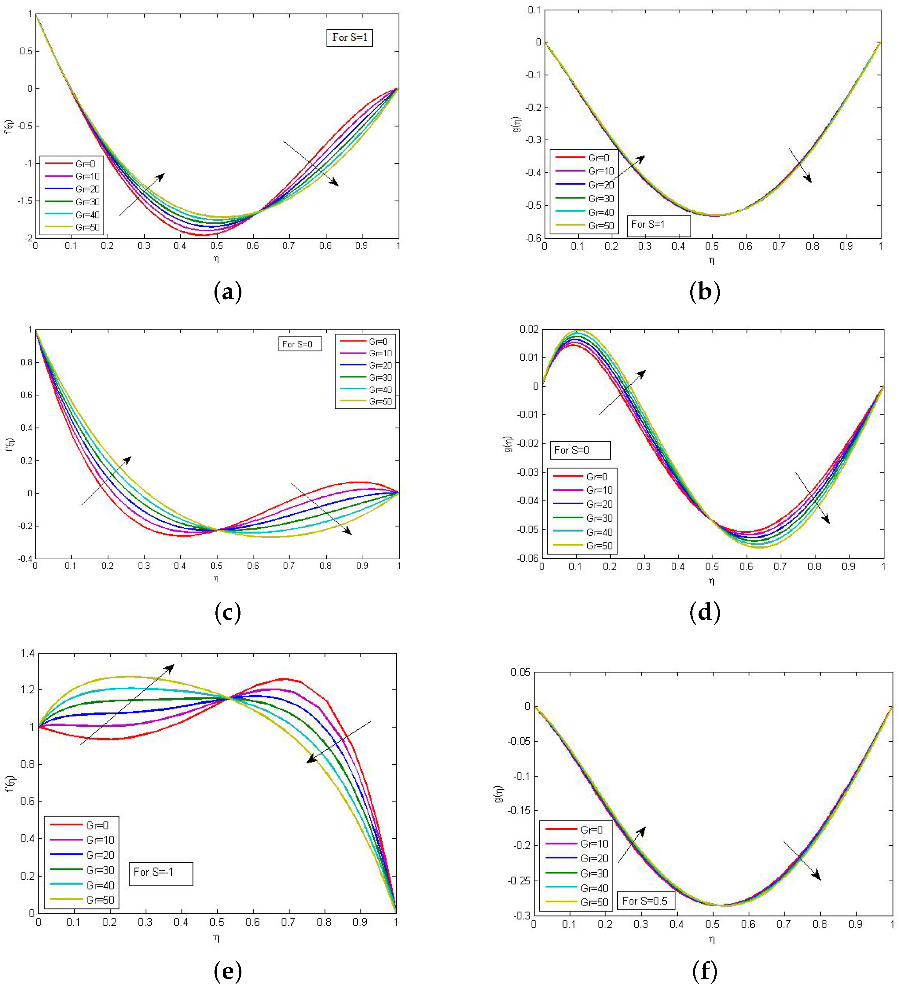
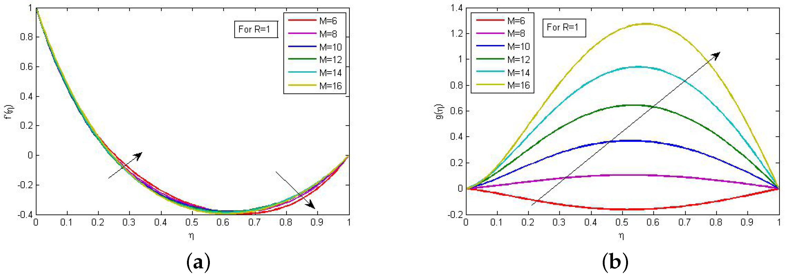
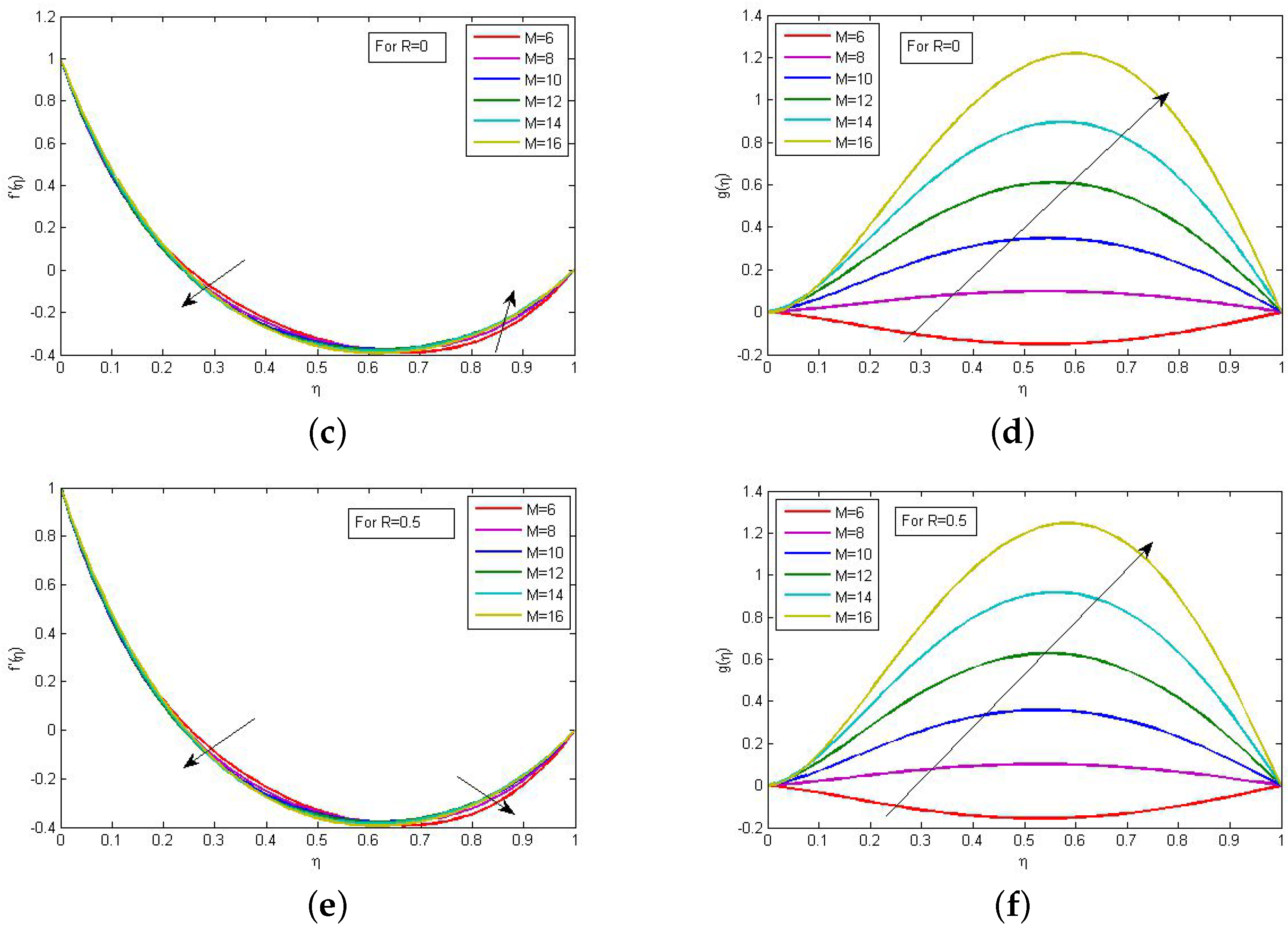
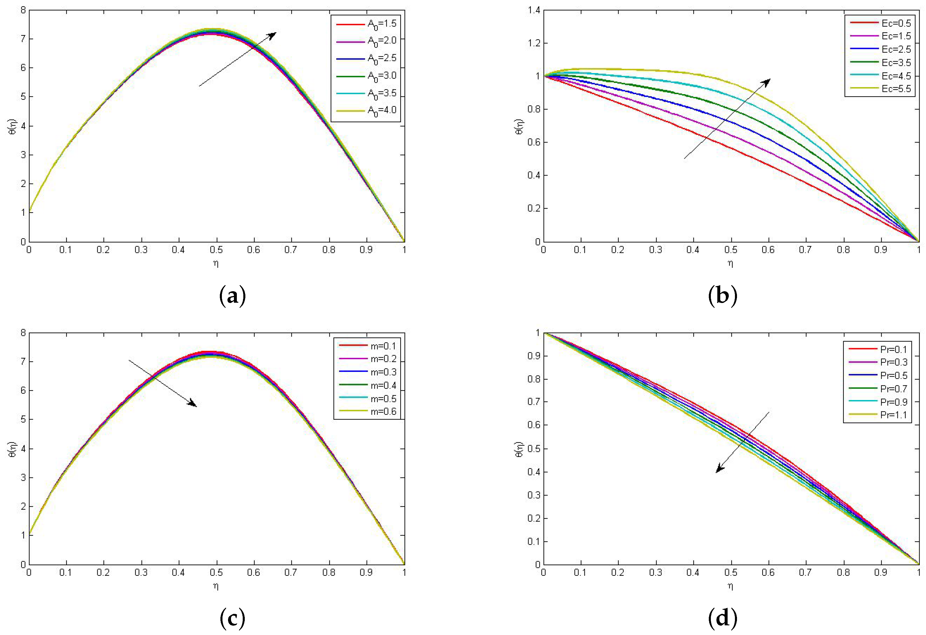
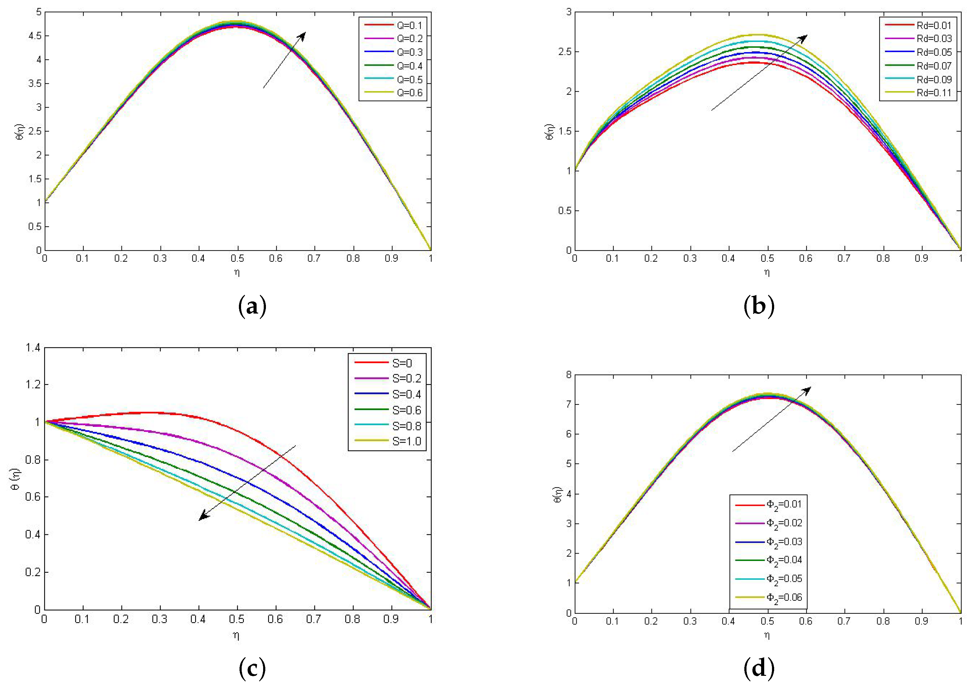
5. Results and Discussion

This portion deals with the discussion and explanation of the results which are obtained during the investigation through graphs and tables. These graphs and tables are displayed by plotting the state variables with varying values of the pertinent parameters of physical interest. These parameters include magnetic parameters, rotation parameters, couple stress parameters, nanomaterials’ concentrations, radiation parameters, the Grahsof number, the Eckert number, etc.
The variation of the velocity components with changing values of the the Grashof number ( G r ) is depicted in Figure 2. The selected G r values are 0.0 , 10 , 20 , 30 , 40 , 50 . This figure consists of six subplots. The left panel from top to bottom shows f ( η ) dependence on G r of the three different cases: (a) Injection ( S = 1.0 ) (b) ( S = 0.0 ) and (c) Suction ( S = 1.0 ). The right panel displays the variation of g ( η ) with G r for the same three cases as the left panel. All these subplots show that the velocity components increases with enhancing G r for smaller η values, while they drop at η larger values. Physically, when the temperature difference increases, it enhances the internal energy of the nanoparticles, and as a result the Brownian motion pumps up, which causes an increase in the migration of the fluid. The f ( η ) variation is more prominent with increasing G r compared to the variation in g ( η ) . Hence, the enhancing buoyancy associated with G r values results in a velocity upsurge near the hot wall, whereas opposite effects are observed at larger distances from the hot wall.
The effect of changing magnetic field parameter M on the velocity components is depicted in Figure 3. The parameter M values are 6 , 8 , 10 , 12 , 14 , 16 . The subplots of the left panel show f ( η ) variation with varying M for the cases: (a) R = 1.0 (b) R = 0.0 . and (c) R = 0.5 . The right column shows the variation of g ( η ) with varying M for the same three cases. The left panel subplots display the enhancing strength of the radiation source change the fluid velocity distribution. When R = 0 , the augmenting values of M drop the velocity component f ( η ) near the boundary layer, while augmenting far away from the boundary layer region. Physically, the magnetic parameter is applied orthogonally to the surface of the fluid flow, as the magnetic field increases the current produced, which acts opposite to the fluid motion, and as a result the fluid velocity at the surface declines. As we move away from the surface, this effect decreases and the magnetic field favours the fluid motion.
The effect of G r and M varying magnitudes on the components of velocity are depicted in Figure 4. The G r chosen values are 0 , 10 , 20 , 30 , 40 , 50 , whereas those of M are M = 6 , 8 , 10 , 12 , 14 , 16 . The subplots of the left panel depict the f ( η ) variation with varying G r for the cases: (a) S = 1.0 (c) S = 0.0 . and (e) S = −1. The right column shows the f ( η ) variation with varying M for cases: (b) R = 1.0 (b) R = 0.0 and (f) R = 0.5 . The left panel subplots display that the gradient in velocity distribution rises in all the three cases with the increasing G r values. The middle subplot of the left panel shows that the velocity distribution increases at a higher rate compared to the injection or suction cases in the first and the last subplots of the left panel. The right panel shows that the gradient in the distribution of velocity lowers with the higher magnetic forces due to higher values of M for the varying strength of the radiation source.
The impact of the varying strength of S and m on the velocity components is exhibited in Figure 5. The selected values of S and m are 0.0 , 0.1 , 0.2 , 0.3 , 0.4 , 0.5 , 0.6 . The subplots of the left panel display of f ( η ) variation with varying (a) S and (c) m. The right column shows the variation of g ( η ) with varying (b) S and (d) m. The left panel subplots display that the gradient in velocity distribution augments with the increasing strength of injection. The subplot (c) shows that the velocity distribution has dual display with varying m. Initially, the velocity distribution declines with enhancing m from η = 0.35 to η = 0.75 , and augments from η = 0.75 to η = 1.00 . The right panel shows that g ( η ) drops with rising strength of S and rises with increasing m values.
The influence of changing strength of S, k r , M, and Φ over the gradient in velocity distribution is shown in Figure 6. The selected values of S are 0.0 , 0.1 , 0.2 , 0.3 , 0.4 , 0.5 , 0.6 , and of k r are 0 , 2 , 4 , 6 , 8 , 10 , M are 6 , 8 , 10 , 12 , 14 , and Φ 1 = Φ 2 are 0.01 , 0.02 , 0.03 , 0.04 , 0.05 , 0.06 . The subplots of the left panel display the variation of f ( η ) with varying (a) S (c) M. The right column shows the variation of f ( η ) with varying (b) k r (d) nanomaterial concentrations Φ 1 , Φ 2 . The left panel subplots display that the gradient in velocity distribution drops with the increasing strength of injection. The subplot (c) shows that the velocity distribution has dual dependence on the varying strength of M. Initially, the velocity distribution augments with increasing M from η = 0.15 to η = 0.55 , and drops from η = 0.6 to η = 0.98 . The upper subplot of the right panel shows that the gradient in velocity distribution drops with the increasing strength of k r and rises with increasing m values. Subplot (d) displays dual dependence of f ( η ) over the increasing concentration of the chosen nanomaterials. For smaller values of η , the gradient rises, while it drops for η higher values.
The impact of varying strength of A 0 , E c , m, and P r on the hybrid nanofluid temperature distribution is exhibited in Figure 7. The chosen strength of A 0 are 1.5 , 2.0 , 2.5 , 3.0 , 3.5 . 4 , 4.0 , of E c are 0.5 , 1.5 , 2.5 , 3.5 , 4.5 , 5.5 , of m are 0.1 , 0.2 , 0.3 , 0.4 , 0.5 , 0.6 , and of P r are 0.1 , 0.3 , 0.5 , 0.7 , 0.9 , 1.1 . The subplots of the left panel display the variation of Θ ( η ) with varying (a) A 0 (c) m. The subplots of the first panel display the temperature enhancement with the A 0 and E c ’s higher values. The enhancement rate of Θ ( η ) with higher values of E c is much larger compared with A 0 higher values. The subplots of the lower row show a drop in temperature with the m and P r increasing values. The dropping rate is more prominent with the increasing P r values. This prominent impact is due to the thermal conductivity of the fluid because, when thermal conductivity declines, the motion of the nanoparticles decreases, which further declines the particles’ interaction, and as a result, the migration of heat reduces.
The impact of the varying strength of Q, R d , S, and ϕ 2 on the temperature distribution of HN is plotted in Figure 8. All these subplots show temperature enhancement with the enhancing strength of the associated variables, except with the increasing strength of injection parameter. This reverse impact of the injection parameter is due to the increase in the viscosity of the fluid which increases the inner molecular bonds’ strength, which as a result causes a decline in the transfer of heat. Similarly, with the increase in the nanoparticles concentration, the Brownian motion increases, which as a result increases the transfer of heat.
Table 3 shows the variation of C f x R e x 0.5 along the x-axis with the changing values of selected parameters. The friction enhances with the rising strength of M, Φ 1 Φ 2 , and k r . The friction displays dual dependence on G r .
Table 4 shows the Nusselt number ( N u x R e x 0.5 ) variation with changing values of the selected quantities. The table shows that the heat transfer through convection enhances with higher values of these associated quantities.

6. Conclusions

This section summarizes the current investigation of the selected HN migration between vertical plates in the presence of magnetic flux, a heat source and radiation The right plate of the configuration is stretching, rotating, and is permeable. The fluid flow is structured by coupled nonlinear PDEs satisfying appropriate boundary conditions. A set of coupled nonlinear ODEs is achieved by using appropriate transformations. The final system is solved with the help of the built in bv4c solver. The variation of state variables with the changing strength of associated parameters is examined graphically and through tables. This work may be extended to other models, and can be analyzed using different hybrid nanofluids. As a limiting case, this work is carried out for a single hybrid nanofluid. The concluding remarks are given as follows:
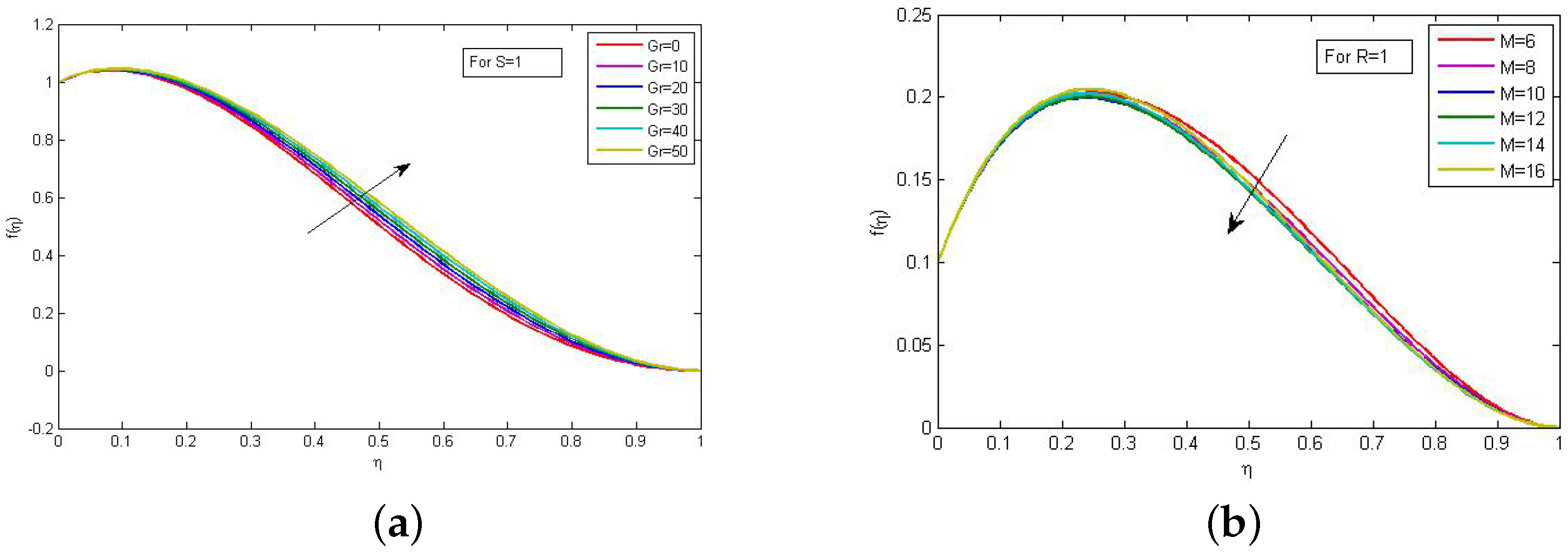
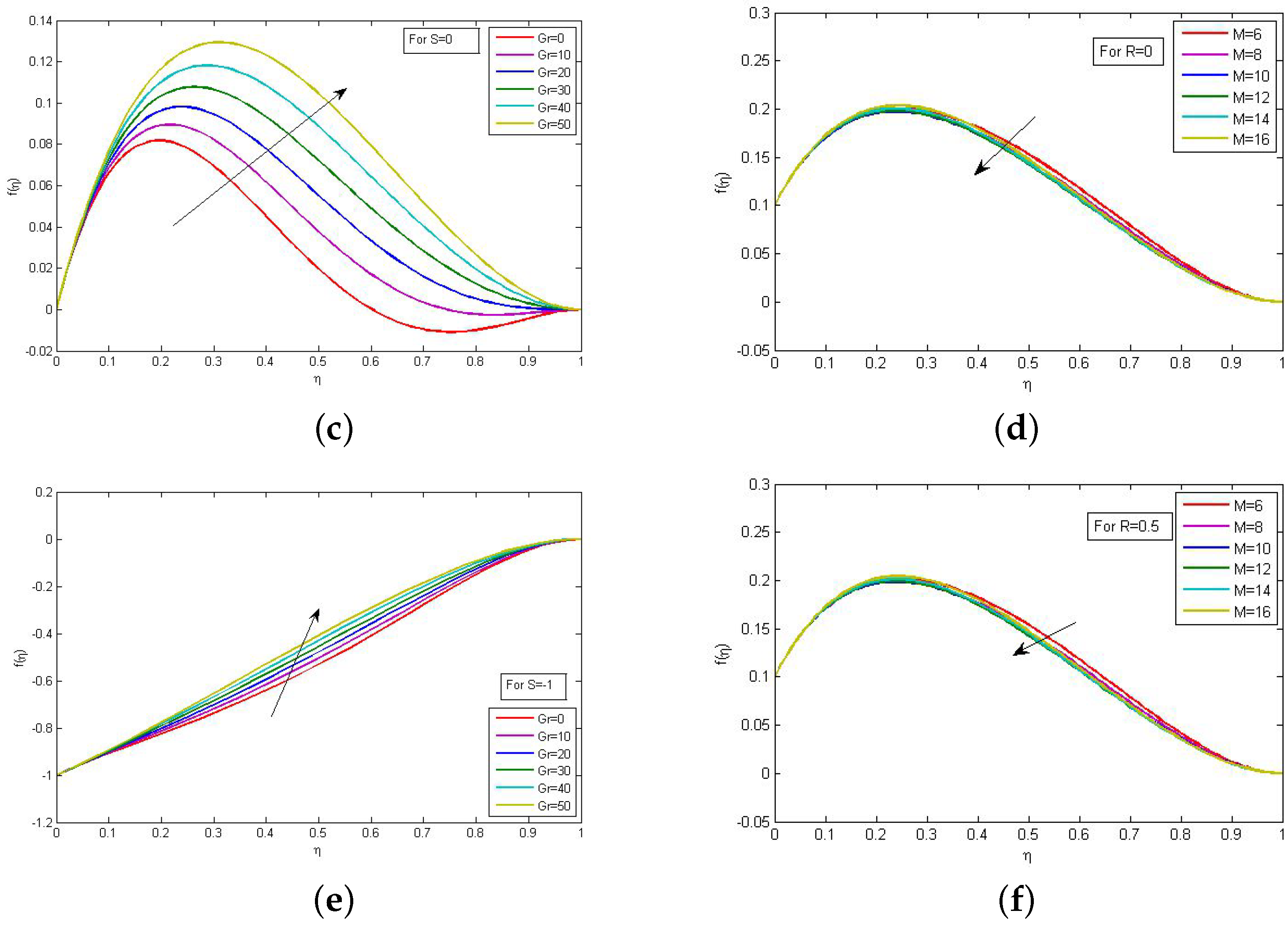
  • It is observed that the velocity distribution initially augments and then decreases with increasing Grashof number values in suction as well as injection.
  • The rising M values first augment and then drop the velocity distribution in the presence of a radiation source of maximum strength.
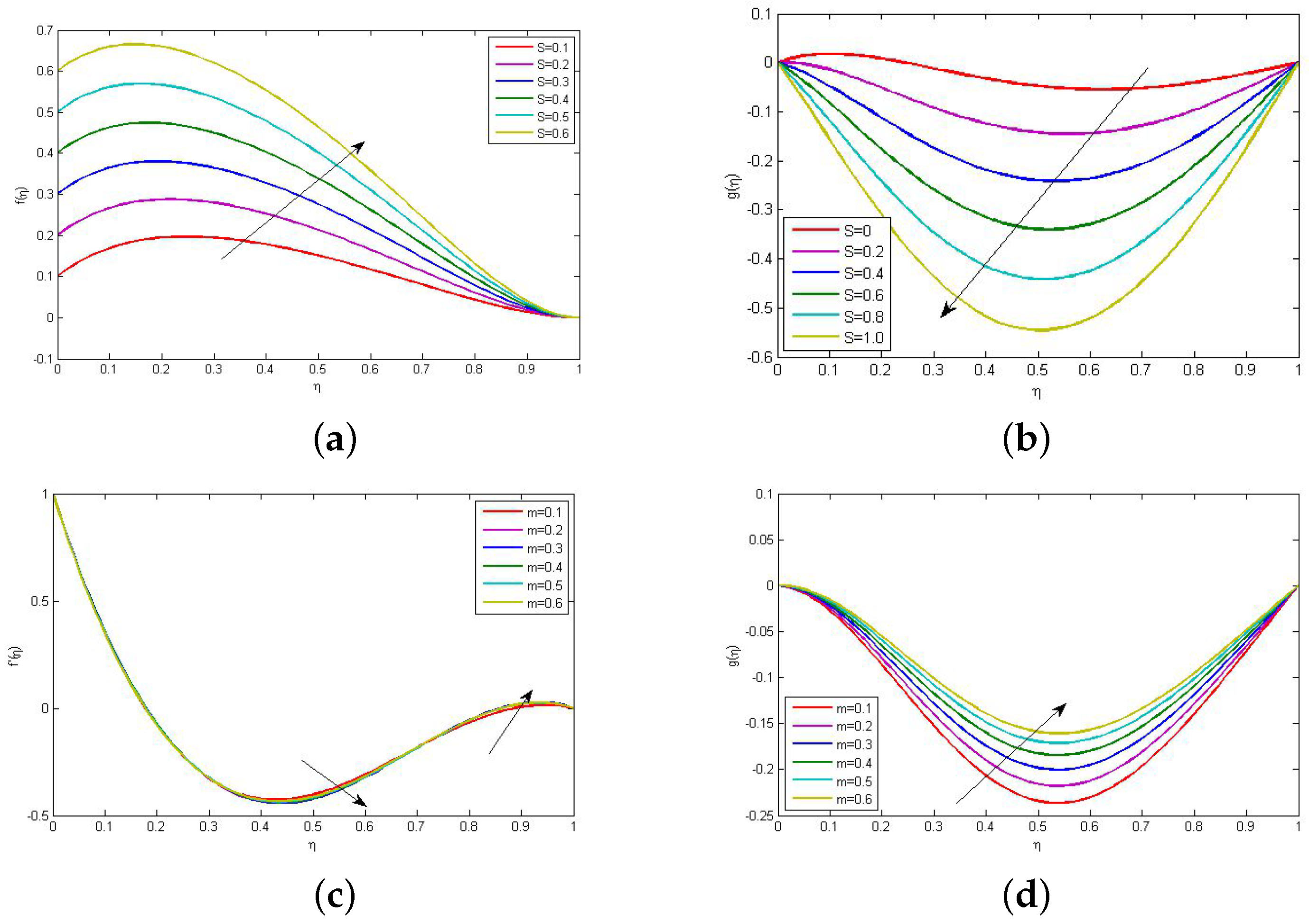
  • The increasing strength of the injection parameter drops the velocity distribution.
  • The temperature increases with the increasing Eckert number, radiation and heat sources’ strength and nanomaterial concentration, and declines with the larger values of injection and Prandtl parameter.
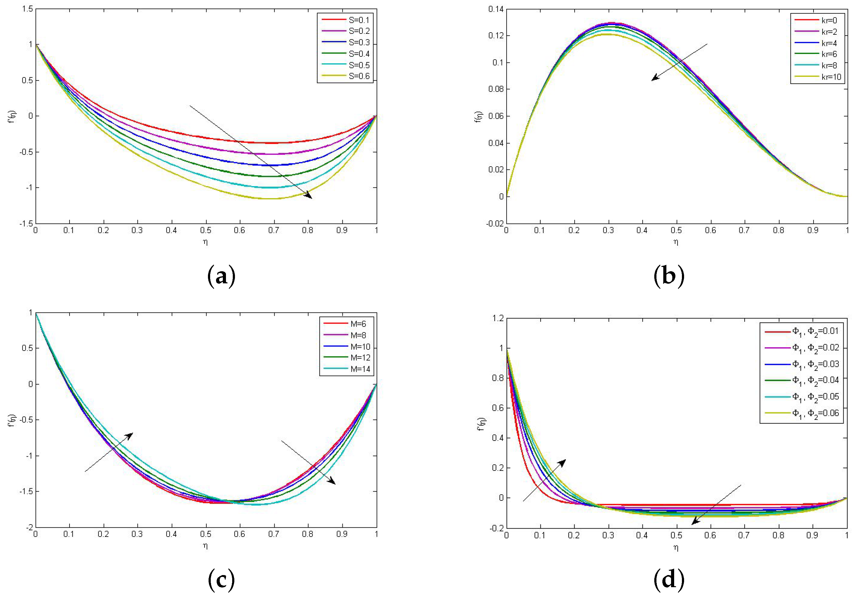
  • The skin friction rises with M and nanomaterial concentrations, and drops with the larger Grashof number values.
  • The heat energy transport due to convection enhances with the rising strength of the pertinent parameters.

Author Contributions

Conceptualization, N.F., S.E. and A.U.; Software, K.A.M.A., I., W.K. and A.U.; Writing—Original Draft Preparation, A.U., S.E. and K.A.M.A.; Writing—Review and Editing, K.A.M.A., I., W.K. and A.U.; Formal Analysis, A.U., K.A.M.A., N.F. and I.; Validation, A.U., K.A.M.A., W.K., S.E. and N.F.; Methodology, A.U., N.F. and K.A.M.A.; Investigation, I., W.K. and A.U.; Resources, A.U., K.A.M.A., I. and N.F.; Project Administration, A.U., N.F. and S.E.; Funding Acquisition, S.E. and N.F. All authors have read and agreed to the published version of the manuscript.

Funding

This research received no external funding.

Data Availability Statement

The data used to support the findings of this study are available within the article.

Acknowledgments

Princess Nourah bint Abdulrahman University Researchers Supporting Project number (PNURSP2023R163), Princess Nourah bint Abdulrahman University, Riyadh, Saudi Arabia. The author N.F. would like to thank Prince Sultan University for paying the publication fees (APC) for this work through TAS LAB.

Conflicts of Interest

The authors declare no conflict of interest.

Abbreviations

Following abbreviations are used in this study:
γ 0 Porosity parameter
β Thermal expansion coefficient
G r Grashof number
QHeat source/sink parameter
R d Radiation parameter
k r Rotational parameter
E c Eckert number
k 1 Absorption coefficient
k r Rotational parameter
σ s Stefan constant
σ Electrical conductivity S m
B ( t ) Time defendant magnetic parameter
B 0 Magnetic field strength
Ω Rotation angle
U w Stretching velocity m sec
V w Velocity of suction/injection mass transfer m sec
ρ h n f Hybrid nanofluid density ( kg m 3 )
μ h n f Hybrid nanofluid dynamic viscosity mPa
ν h n f Hybrid nanofluid kinematic viscosity m 2 s
k h n f Hybrid nanofluid thermal conductivity
σ h n f Hybrid nanofluid electrical conductivity
ϵ 1 , ϵ 2 , ϵ 3 , ϵ 4 , ϵ 5 and A 0 Dimensionless constants
N u x Local Nusslet number
R e x Local Reynolds number
C f x Local Skin friction
P r Prandtl number
TFluid temperature (K)
C p Specific heat ( J kg K )
fDimensionless velocity
gDimensionless velocity
θ Dimensionless temperature
Condition at infinity
hReference condition
x, y, and zCoordinates (m)
η Similarity variable
tTime (s)
mHall parameter
SSuction/injection parameter
Φ 1 , Φ 2                   First and second nanoaprticles volume fractions
HNHybrid nanofluid
B.Cs.Hybrid nanofluid
PDEsPartial differential equations
ODEsOrdinary differential equations
MMagnetic field interaction parameter

References

  1. Alsabery, A.; Chamkha, A.; Saleh, H.; Hashim, I. Natural convection flow of a nanofluid in an inclined square enclosure partially filled with a porous medium. Sci. Rep. 2017, 7, 1–18. [Google Scholar] [CrossRef] [PubMed] [Green Version]
  2. Xu, H.J.; Xing, Z.B.; Wang, F.; Cheng, Z. Review on heat conduction, heat convection, thermal radiation and phase change heat transfer of nanofluids in porous media: Fundamentals and applications. Chem. Eng. Sci. 2019, 195, 462–483. [Google Scholar] [CrossRef]
  3. Choi, S.U.; Eastman, J.A. Enhancing Thermal Conductivity of Fluids with Nanoparticles; Technical Report; Argonne National Lab.: Lemont, IL, USA, 1995. [Google Scholar]
  4. Al-Srayyih, B.M.; Gao, S.; Hussain, S.H. Effects of linearly heated left wall on natural convection within a superposed cavity filled with composite nanofluid-porous layers. Adv. Powder Technol. 2019, 30, 55–72. [Google Scholar] [CrossRef]
  5. Mehryan, S.; Ghalambaz, M.; Izadi, M. Conjugate natural convection of nanofluids inside an enclosure filled by three layers of solid, porous medium and free nanofluid using Buongiorno’s and local thermal non-equilibrium models. J. Therm. Anal. Calorim. 2019, 135, 1047–1067. [Google Scholar] [CrossRef]
  6. Khanafer, K.; Vafai, K. A review on the applications of nanofluids in solar energy field. Renew. Energy 2018, 123, 398–406. [Google Scholar] [CrossRef]
  7. Basha, H.T.; Sivaraj, R.; Reddy, A.S.; Chamkha, A. SWCNH/diamond-ethylene glycol nanofluid flow over a wedge, plate and stagnation point with induced magnetic field and nonlinear radiation–solar energy application. Eur. Phys. J. Spec. Top. 2019, 228, 2531–2551. [Google Scholar] [CrossRef]
  8. Izadi, A.; Siavashi, M.; Xiong, Q. Impingement jet hydrogen, air and CuH2O nanofluid cooling of a hot surface covered by porous media with non-uniform input jet velocity. Int. J. Hydrog. Energy 2019, 44, 15933–15948. [Google Scholar] [CrossRef]
  9. Sabaghan, A.; Edalatpour, M.; Moghadam, M.C.; Roohi, E.; Niazmand, H. Nanofluid flow and heat transfer in a microchannel with longitudinal vortex generators: Two-phase numerical simulation. Appl. Therm. Eng. 2016, 100, 179–189. [Google Scholar] [CrossRef]
  10. Ebrahimi, A.; Rikhtegar, F.; Sabaghan, A.; Roohi, E. Heat transfer and entropy generation in a microchannel with longitudinal vortex generators using nanofluids. Energy 2016, 101, 190–201. [Google Scholar] [CrossRef]
  11. Siavashi, M.; Joibary, S.M.M. Numerical performance analysis of a counter-flow double-pipe heat exchanger with using nanofluid and both sides partly filled with porous media. J. Therm. Anal. Calorim. 2019, 135, 1595–1610. [Google Scholar] [CrossRef]
  12. Ghadikolaei, S.; Hosseinzadeh, K.; Ganji, D.; Jafari, B. Nonlinear thermal radiation effect on magneto Casson nanofluid flow with Joule heating effect over an inclined porous stretching sheet. Case Stud. Therm. Eng. 2018, 12, 176–187. [Google Scholar] [CrossRef]
  13. Kumar, M.A.; Reddy, Y.D.; Rao, V.S.; Goud, B.S. Thermal radiation impact on MHD heat transfer natural convective nano fluid flow over an impulsively started vertical plate. Case Stud. Therm. Eng. 2021, 24, 100826. [Google Scholar] [CrossRef]
  14. Naranjani, B.; Roohi, E.; Ebrahimi, A. Thermal and hydraulic performance analysis of a heat sink with corrugated channels and nanofluids. J. Therm. Anal. Calorim. 2020, 146, 2549–2560. [Google Scholar] [CrossRef]
  15. Mebarek-Oudina, F. Convective heat transfer of Titania nanofluids of different base fluids in cylindrical annulus with discrete heat source. Heat Transf. Res. 2019, 48, 135–147. [Google Scholar] [CrossRef] [Green Version]
  16. Muhammad, T.; Alamri, S.Z.; Waqas, H.; Habib, D.; Ellahi, R. Bioconvection flow of magnetized Carreau nanofluid under the influence of slip over a wedge with motile microorganisms. J. Therm. Anal. Calorim. 2021, 143, 945–957. [Google Scholar] [CrossRef]
  17. Fatima, N. New homotopy perturbation method for solving nonlinear differential equations and Fisher type equation. In Proceedings of the 2017 IEEE International Conference on Power, Control, Signals and Instrumentation Engineering (ICPCSI), Chennai, India, 21–22 September 2017; pp. 1669–1673. [Google Scholar]
  18. Saif, R.S.; Hayat, T.; Ellahi, R.; Muhammad, T.; Alsaedi, A. Darcy–Forchheimer flow of nanofluid due to a curved stretching surface. Int. J. Numer. Methods Heat Fluid Flow 2019, 29, 2–20. [Google Scholar] [CrossRef]
  19. Khan, A.A.; Naeem, S.; Ellahi, R.; Sait, S.M.; Vafai, K. Dufour and Soret effects on Darcy-Forchheimer flow of second-grade fluid with the variable magnetic field and thermal conductivity. Int. J. Numer. Methods Heat Fluid Flow 2020, 30, 4331–4347. [Google Scholar] [CrossRef]
  20. Qasim, M.; Khan, Z.H.; Khan, W.A.; Ali Shah, I. MHD boundary layer slip flow and heat transfer of ferrofluid along a stretching cylinder with prescribed heat flux. PLoS ONE 2014, 9, e83930. [Google Scholar] [CrossRef]
  21. Afridi, M.I.; Qasim, M. Entropy generation in three dimensional flow of dissipative fluid. Int. J. Appl. Comput. Math. 2018, 4, 1–11. [Google Scholar] [CrossRef]
  22. Qasim, M. Heat and mass transfer in a Jeffrey fluid over a stretching sheet with heat source/sink. Alex. Eng. J. 2013, 52, 571–575. [Google Scholar] [CrossRef]
  23. Mahalakshmi, T.; Nithyadevi, N.; Oztop, H.F.; Abu-Hamdeh, N. MHD mixed convective heat transfer in a lid-driven enclosure filled with Ag-water nanofluid with center heater. Int. J. Mech. Sci. 2018, 142, 407–419. [Google Scholar] [CrossRef]
  24. Sheikholeslami, M.; Rezaeianjouybari, B.; Darzi, M.; Shafee, A.; Li, Z.; Nguyen, T.K. Application of nano-refrigerant for boiling heat transfer enhancement employing an experimental study. Int. J. Heat Mass Transf. 2019, 141, 974–980. [Google Scholar] [CrossRef]
  25. Zhang, L.; Bhatti, M.M.; Ellahi, R.; Michaelides, E.E. Oxytactic microorganisms and thermo-bioconvection nanofluid flow over a porous Riga plate with Darcy–Brinkman–Forchheimer medium. J. Non-Equilib. Thermodyn. 2020, 45, 257–268. [Google Scholar] [CrossRef]
  26. Kumar, P.; Poonia, H.; Ali, L.; Areekara, S. The numerical simulation of nanoparticle size and thermal radiation with the magnetic field effect based on tangent hyperbolic nanofluid flow. Case Stud. Therm. Eng. 2022, 37, 102247. [Google Scholar] [CrossRef]
  27. Shutaywi, M.; Shah, Z. Mathematical Modeling and numerical simulation for nanofluid flow with entropy optimization. Case Stud. Therm. Eng. 2021, 26, 101198. [Google Scholar] [CrossRef]
  28. Taylor-Pashow, K.M.; Della Rocca, J.; Huxford, R.C.; Lin, W. Hybrid nanomaterials for biomedical applications. Chem. Commun. 2010, 46, 5832–5849. [Google Scholar] [CrossRef] [PubMed]
  29. Babazadeh, H.; Shah, Z.; Ullah, I.; Kumam, P.; Shafee, A. Analysis of hybrid nanofluid behavior within a porous cavity including Lorentz forces and radiation impacts. J. Therm. Anal. Calorim. 2020, 143, 1129–1137. [Google Scholar] [CrossRef]
  30. Mehryan, S.; Izadpanahi, E.; Ghalambaz, M.; Chamkha, A. Mixed convection flow caused by an oscillating cylinder in a square cavity filled with Cu–Al2O3/water hybrid nanofluid. J. Therm. Anal. Calorim. 2019, 137, 965–982. [Google Scholar] [CrossRef]
  31. Suresh, S.; Venkitaraj, K.; Selvakumar, P.; Chandrasekar, M. Synthesis of Al2O3–Cu/water hybrid nanofluids using two step method and its thermo physical properties. Colloids Surf. A Physicochem. Eng. Asp. 2011, 388, 41–48. [Google Scholar] [CrossRef]
  32. Chamkha, A.J.; Miroshnichenko, I.V.; Sheremet, M.A. Numerical analysis of unsteady conjugate natural convection of hybrid water-based nanofluid in a semicircular cavity. J. Therm. Sci. Eng. Appl. 2017, 9, 041004. [Google Scholar] [CrossRef]
  33. Momin, G.G. Experimental investigation of mixed convection with water-Al2O3 & hybrid nanofluid in inclined tube for laminar flow. Int. J. Sci. Technol. Res. 2013, 2, 195–202. [Google Scholar]
  34. Qadeer, M.; Khan, U.; Ahmad, S. Irreversibility analysis for three-dimensional squeezing flow of hybrid nanofluids: A numerical study. Waves Random Complex Media 2022, 1–27. [Google Scholar] [CrossRef]
  35. Sundar, L.S.; Singh, M.K.; Sousa, A.C. Enhanced heat transfer and friction factor of MWCNT–Fe3O4/water hybrid nanofluids. Int. Commun. Heat Mass Transf. 2014, 52, 73–83. [Google Scholar] [CrossRef]
  36. Ghachem, K.; Aich, W.; Kolsi, L. Computational analysis of hybrid nanofluid enhanced heat transfer in cross flow micro heat exchanger with rectangular wavy channels. Case Stud. Therm. Eng. 2021, 24, 100822. [Google Scholar] [CrossRef]
  37. Lund, L.A.; Omar, Z.; Khan, I.; Seikh, A.H.; Sherif, E.S.M.; Nisar, K.S. Stability analysis and multiple solution of Cu–Al2O3/H2O nanofluid contains hybrid nanomaterials over a shrinking surface in the presence of viscous dissipation. J. Mater. Res. Technol. 2020, 9, 421–432. [Google Scholar] [CrossRef]
  38. Suresh, S.; Venkitaraj, K.; Selvakumar, P.; Chandrasekar, M. Effect of Al2O3–Cu/water hybrid nanofluid in heat transfer. Exp. Therm. Fluid Sci. 2012, 38, 54–60. [Google Scholar] [CrossRef]
  39. Afridi, M.; Qasim, M.; Khan, N.A.; Hamdani, M. Heat transfer analysis of Cu–Al2O3–water and Cu–Al2O3–kerosene oil hybrid nanofluids in the presence of frictional heating: Using 3-stage Lobatto IIIA formula. J. Nanofluids 2019, 8, 885–891. [Google Scholar] [CrossRef]
  40. Usman, M.; Hamid, M.; Zubair, T.; Haq, R.U.; Wang, W. Cu-Al2O3/Water hybrid nanofluid through a permeable surface in the presence of nonlinear radiation and variable thermal conductivity via LSM. Int. J. Heat Mass Transf. 2018, 126, 1347–1356. [Google Scholar] [CrossRef]
  41. Mohebbi, R.; Izadi, M.; Delouei, A.A.; Sajjadi, H. Effect of MWCNT–Fe3O4/water hybrid nanofluid on the thermal performance of ribbed channel with apart sections of heating and cooling. J. Therm. Anal. Calorim. 2019, 135, 3029–3042. [Google Scholar] [CrossRef]
  42. Minea, A.; Moldoveanu, M. Overview of hybrid nanofluids development and benefits. J. Eng. Thermophys. 2018, 27, 507–514. [Google Scholar] [CrossRef]
  43. Abdeljawad, T.; Ullah, A.; Alrabaiah, H.; Ikramullah; Ayaz, M.; Khan, W.; Khan, I.; Khan, H.U. Thermal radiations and mass transfer analysis of the three-dimensional magnetite carreau fluid flow past a horizontal surface of paraboloid of revolution. Processes 2020, 8, 656. [Google Scholar] [CrossRef]
  44. Rizk, D.; Ullah, A.; Elattar, S.; Alharbi, K.A.M.; Sohail, M.; Khan, R.; Khan, A.; Mlaiki, N. Impact of the KKL Correlation Model on the Activation of Thermal Energy for the Hybrid Nanofluid (GO+ ZnO+ Water) Flow through Permeable Vertically Rotating Surface. Energies 2022, 15, 2872. [Google Scholar] [CrossRef]
  45. Sinha, A.; Misra, J.; Shit, G. Effect of heat transfer on unsteady MHD flow of blood in a permeable vessel in the presence of non-uniform heat source. Alex. Eng. J. 2016, 55, 2023–2033. [Google Scholar] [CrossRef] [Green Version]
  46. Khashi’ie, N.S.; Waini, I.; Arifin, N.M.; Pop, I. Unsteady squeezing flow of Cu-Al2O3/water hybrid nanofluid in a horizontal channel with magnetic field. Sci. Rep. 2021, 11, 1–11. [Google Scholar] [CrossRef] [PubMed]
  47. Riahi, A.; Ben-Cheikh, N.; Campo, A. Water-based nanofluids for natural convection cooling of a pair of symmetrical heated blocks placed inside a rectangular enclosure of aspect ratio two. Int. J. Therm. Environ. Eng. 2018, 16, 1–10. [Google Scholar]
  48. Verma, V.K.; Mondal, S. A brief review of numerical methods for heat and mass transfer of Casson fluids. Partial Differ. Equations Appl. Math. 2021, 3, 100034. [Google Scholar] [CrossRef]
  49. Rai, N.; Mondal, S. Spectral methods to solve nonlinear problems: A review. Partial Differ. Equations Appl. Math. 2021, 4, 100043. [Google Scholar] [CrossRef]
  50. Oyelakin, I.S.; Mondal, S.; Sibanda, P.; Motsa, S.S. A multi-domain bivariate approach for mixed convection in a Casson nanofluid with heat generation. Walailak J. Sci. Technol. 2019, 16, 681–699. [Google Scholar] [CrossRef]
Figure 1. Problem geometry.
Energies 16 01220 g001
Figure 2. Influence of G r on f ( η ) for cases (a) S = 1.0 (c) S = 0.0 (e) S = −1.0, and influence of G r on g ( η ) for cases (b) S = 1.0 (d) S = 0.0 (f) S =  −1.0.
Energies 16 01220 g002
Figure 3. Impact of M on f ( η ) for cases (a) R = 1.0 (c) R = 0.0 (e) S = 0.5 , and of M on g ( η ) for cases (b) R = 1.0 (d) R = 0.0 (f) R = 0.5 .
Energies 16 01220 g003aEnergies 16 01220 g003b
Figure 4. Effect of G r on f ( η ) for cases (a) S = 1.0 (c) S = 0.0 (e) S = 1 , and of M over f ( η ) for cases (b) R = 1.0 (d) R = 0.0 (f) R = 0.5 .
Energies 16 01220 g004aEnergies 16 01220 g004b
Figure 5. Dependence of (a) S on f ( η ) (c) m on f ( η ) (b) S on g ( η ) (d) m on g ( η ) , respectively.
Energies 16 01220 g005
Figure 6. Effect of (a) S (c) M (b) k r and (d) Φ 1 , Φ 2 on f ( η ) .
Energies 16 01220 g006
Figure 7. (a) Influence of A 0 , (b) S c on, (c) m, and (d) P r on θ ( η ) .
Energies 16 01220 g007
Figure 8. Influence of (a) Q, (b) R d (c) S and (d) ϕ 2 on Θ ( η ) .
Energies 16 01220 g008
Table 1. Physical characteristics of silver (Ag), titanium dioxide (TiO 2 ) and water [47].
Properties k W m · K æ Kg m 3 C p J Kg · K
Ag42910.5235
Water0.613997.14179
TiO 2 8.954250686
Table 2. Mathematical relations for the computation of physical properties of HN [46].
QuantityHybrid Models
Thermal Conductivity k h n f k b f = ( 1 Φ 2 ) + 2 Φ 2 k m 2 k m 2 k b f l n k m 2 + k b f 2 k b f
k b f k f = ( 1 Φ 1 ) + 2 Φ 1 k m 1 k m 1 k f l n k m 1 + k f 2 k f
Electrical Conductivity σ h n f σ b f = 1 + 3 σ m 2 σ b f 1 Φ 2 σ m 2 σ b f + 2 σ m 2 σ b f 1 Φ 2
σ b f σ f = 1 + 3 σ m 1 σ f 1 Φ 1 σ m 1 σ f + 2 σ m 1 σ f 1 Φ 1
Specific Heat ( ρ C p ) h n f ( ρ C p ) f = ( 1 Φ 2 ) 1 1 ( ρ C p ) m 1 ( ρ C p ) f Φ 1 + Φ 2 ( ρ C p ) m 2 ( ρ C p ) f
Viscosity μ h n f μ f = 1 ( 1 Φ 1 ) 2.5 ( 1 Φ 2 ) 2.5
Density ρ h n f ρ f = ( 1 Φ 2 ) 1 1 ρ m 1 ρ f Φ 1 + Φ 2 ρ m 2 ρ f
Table 3. Depenedence of C f x R e x 0.5 values with the varying strength of associated quantities [44].
M Φ 1 Φ 2 kr Gr Cf x
0.10.010.10.11.35340
0.3 1.56322
0.50.02 1.61480
0.04 1.70841
0.5 1.81831
0.3 1.88298
0.51.80101
0.71.67691
Table 4. Dependence of N u x R e x 0.5 on different quantities [44].
Φ 1 Φ 2 MQ Rd Ec Pr Nu x
0.020.10.10.125.00.112352
0.04 0.266434
0.060.3 0.270780
0.5 0.410970
0.4 0.490223
0.8 0.611523
0.4 0.699960
0.8 0.823056
3 0.935024
4 0.999068
5.20.611976
5.30.634667
Disclaimer/Publisher’s Note: The statements, opinions and data contained in all publications are solely those of the individual author(s) and contributor(s) and not of MDPI and/or the editor(s). MDPI and/or the editor(s) disclaim responsibility for any injury to people or property resulting from any ideas, methods, instructions or products referred to in the content.

