Calibration of Grid Models for Analyzing Energy Policies

Abstract

Intermittent forms of renewable energy destabilize electricity grids unless adequate reliable generating capacity and storage are available, while instability of hybrid electricity grids and cost fluctuations in fossil fuel prices pose further challenges for policymakers. We examine the interaction between renewable and traditional fossil-fuel energy sources in the context of the Alberta electricity grid, where policymakers seek to eliminate coal and reduce reliance on natural gas. We develop a policy model of the Alberta grid and, unlike earlier models, calibrate the cost functions of thermal generation using positive mathematical programming. Rather than employing constant average and marginal costs, calibration determines upward sloping supply (marginal cost) functions. The calibrated model is then used to determine an optimal generation mix under different assumptions regarding carbon prices and policies to eliminate coal-fired capacity. Results indicate that significant wind capacity can enter the Alberta grid if carbon prices are high, but that it remains difficult to eliminate reliable baseload capacity. Adequate baseload coal and/or natural gas capacity is required, which is the case even if battery storage is allowed into the system. Further, significant peak-load gas capacity will also be required to backstop intermittent renewables.

1. Introduction

The integration of renewable energy sources into electricity grids can lead to instability due to the variable and intermittent nature of wind and solar power outputs [1,2,3]. This can result in inefficient thermal generation and increased CO₂ emissions when traditional generators are required to ramp up quickly to meet changes in load [4]. Additionally, the low cost of wind and solar generation can negatively impact the profitability of traditional thermal generators, as their capacity factors decrease and they may not generate enough revenue to recover their capital costs [5,6]. Furthermore, when renewable generation falls below expectations, and fossil fuel prices are simultaneously high, it can lead to “green inflation” characterized by a surge in electricity prices and the overall price level [7]. These effects have been observed in Europe in 2022, where lower-than-expected wind regimes have led to increased output from fossil-fuel generators, resulting in higher gas prices and increased electricity prices [8,9].

To better understand the potential impacts of increasing reliance on renewables, electricity system models have been developed to analyze the penetration of renewables into power grids and their impacts on greenhouse gas (GHG) emissions. Dispatch modelling, which represents short-term system operation, and capacity expansion modelling, which represents long-term system investment planning, are the two main methodologies that have been applied. Recent engineering-type models have been developed to examine the least-cost combination of investments in energy technology and the least-cost set of operational choices to meet electricity. Examples include the constrained optimization models GenX [10] and OseMOSYS [11], with [12] providing a review of electricity grid models.

Our model is a policy as opposed to engineering type of model; thus, there is less concern about details regarding individual generators. A policy model assumes that each generation type constitutes a single asset rather than a variety of plants [13]. In this study, a policy-oriented mathematical programming (MP) model is used to determine the optimal generation mix that includes a role for renewable wind and solar assets, and battery storage. It modifies the traditional load-duration-screening-curve method [6], which identifies an optimal generation mix for a set of price and cost parameters, by considering renewable intermittency and its potential impact on other generators. In that case, the optimal generation mix is sensitive to the factors accounting for intermittency, such as wind and solar regimes [14].

The MP model that we modify here was originally developed by Prescott et al. [15]. They examined the potential for wind energy to reduce possible blackouts that might occur in Vancouver Island. As discussed by the authors, one blackout had already occurred, and more were predicted. The integer programming model developed in [15] minimized the cost of generating electricity on the Island by allocating generation across existing assets plus various levels of wind asset availability. Costs were minimized subject to meeting hourly load levels, up- and down-ramping constraints, capacity constraints on existing assets, and a reliability constraint. The results indicated that, while wind power could contribute to overall generation, it could not alleviate future shortfalls because wind power would not always be available at the time needed to prevent a blackout. Following their procedure, our model seeks to determine the best operational and investment strategies to meet the demand for all hours in a year.

The major innovation of our model is the introduction of a calibration procedure, which is necessary to account for the complexities of the electricity grid, such as regulatory and political developments (e.g., command-and-control versus unregulated and privatized decision-making), technological developments, market prices for primary energy carriers, and weather factors (e.g., related to wind and solar output) [16]. The complexity of the MP problem poses many challenges, with a major one related to the costs of operating power plants at various levels of capacity. Information on costs is difficult to find—cost data and (quite sophisticated) decision models used by system operators and asset owners are often proprietary (see [12]). Further, even if costs are available for individual generators, models often aggregate several or all generators of a particular fuel type. In that case, engineering costs are no longer relevant for modelling purposes as costs need to reflect how various generators operate in tandem and how external factors, including the operation of other generator types under changing load conditions, affect operating costs. Policy models of an electricity grid must then be calibrated to actual operating levels, and this requires the discovery of the parameters of economic cost functions. Once calibrated, a model can be used for policy analyses related to, say, a carbon tax or output restrictions on certain classes of generators.

Given that calibration of MP models of electricity grids is not common in the literature, a major contribution of the current research is to demonstrate how one or more calibration methods can be used to develop economic cost functions for grid optimization modelling. As an application, we calibrate the cost functions for fossil fuel generators using data on generation by assets and related prices for a grid characterized by a mix of generating assets but dominated by coal-fired power and various types of natural gas sources (e.g., baseload and peaking gas plants and co-generation assets) and increasing wind capacity. While price data are required for calibrating the model, when simulating the effect of climate policies on generation, prices are no longer available (as they are determined by the mix of assets and generation decisions). Therefore, it is necessary to minimize costs rather than maximize revenue.

A simple and efficient calibration methodology coupled with an optimization model allows us to disentangle the complex interactions of different types of generating assets. It is only after the model has been calibrated that it can be used to examine the effects of different policies on the mix of generation assets comprising an electricity grid. Our application is to the Alberta electricity grid because it consists of substantial fossil fuel assets, especially coal plants, that need to be shuttered in the context of the drive to Net-Zero. In particular, we identify how the overall capacity and generation mix might change as a government implements a carbon tax and emission standards as policy instruments. The Alberta results are representative of what might happen in other jurisdictions, such as Australia, the UK, and various North American systems, despite differences in asset mixes and scale. That is, the proposed methodology can be utilized to study a host of policy scenarios, including changes in generation costs, plant operations, load, and so on.

The remainder of the paper is structured as follows. In the materials and method section, we first discuss methods for calibrating MP models followed by a description of our model. Then, in the results section, we present our findings, including as an intermediate result the calibrated cost functions; some of the results are presented graphically. The conclusion and policy implications section summarize the main findings and discusses implications for policy; here we also provide recommendations for future research.

2. Materials and Methods

2.1. Background: Calibrating Mathematical Programming Models

Before a grid optimization model can be used for policy purposes, it is important to calibrate the parameters used to represent various aspects of the grid so that it is most representative of the actual grid [17]. A well-calibrated MP model should be able to reproduce observed historical data—a model should be calibrated so that it provides a realistic approximation of what happens in the real world [18]. In an MP model, calibration constraints use data on inputs and outputs (for a base year, say) to discover the parameters of a postulated objective functional form so that, once the calibration constraints are removed, the model with the adjusted objective function replicates the observed outcomes ([19,20]). The calibrated models can then be used for policy analysis.

Positive mathematical programming (PMP) is an approach that directly enables one to find the parameters of an economic cost function. PMP has been used to calibrate models in agricultural and resource economics but has yet to be applied to the estimation of cost functions in the operation of electricity grids. The method was first developed by Howitt [19] who derived cost functions based on positive inferences from base year data rather than normative assumptions. PMP uses information about the dual variables associated with the calibration constraints to adjust the objective function so that the calibrated model duplicates observed outcomes. The most common application begins by specifying a linear objective function in the calibration stage but replaces it with a nonlinear (often quadratic) objective function once the model is calibrated. The method was initially applied to policy analysis in agriculture (e.g., [21,22]) but has increasingly been implemented in trade models and models related to resource management [23,24,25].

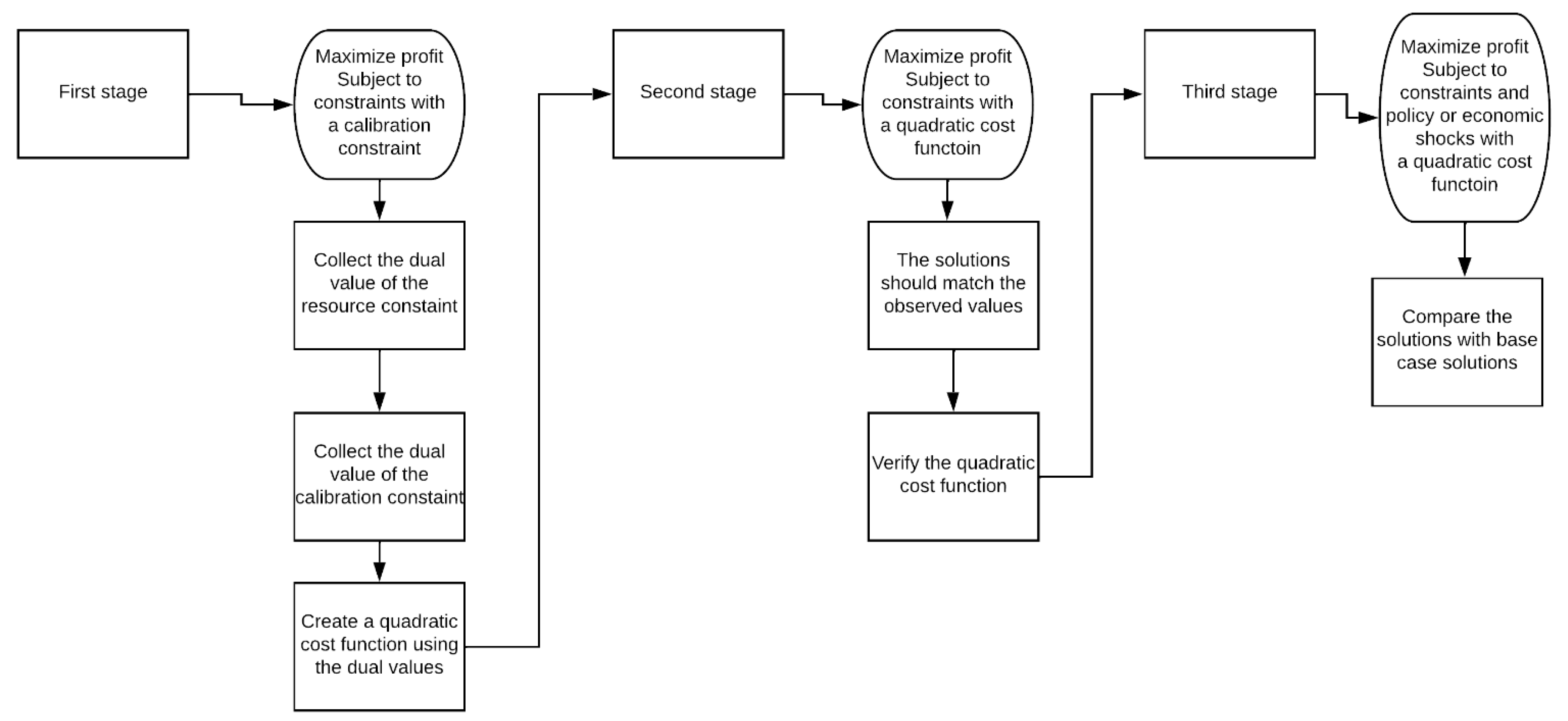
The standard PMP approach involves three stages to calibrate a linear cost function (1st stage), thereby obtaining an upward sloping supply (marginal cost) function (2nd stage), and a 3rd stage where the calibrated model is used to analyze policy. This is illustrated in Figure 1. The optimization problem is defined as:

$$\underset{\mathit{x}}{\mathrm{Maximize}} \mathrm{R}(\mathit{x}) - \mathbf{c}(\mathit{x})$$

(1)

$$\mathrm{Subject} \mathrm{to}: \mathbf{A}\mathit{x} \le \mathbf{b},$$

(2)

where $\mathrm{R}(\mathit{x})$ and $\mathrm{c}(\mathit{x})$ are revenue and cost functions, respectively. The vector $\mathit{x}$ is k × 1, representing k activities with non-negative values; vector $\mathbf{b}$ is m × 1, signifying the m resource constraints; $\mathbf{A}$ is a m × k matrix which specifies the resource usage for each activity. In practice, $\mathrm{c}(\mathit{x})$ represents the average variable costs rather than marginal costs (supply functions) that vary with $\mathit{x}$.

In general, a linear programming (LP) model is specified in the first stage of the PMP process along with calibration constraints that bind the LP problem to the observed activity levels:

$$\underset{\mathit{x}}{\mathrm{Maximize}}\mathrm{Z}=\mathbf{p}’\mathit{x} - \mathbf{c}’\mathit{x}$$

(3)

$$\mathrm{Subject} \mathrm{to}: \mathbf{A}\mathit{x} \le \mathbf{b} \left[\mathit{\lambda }\right],$$

(4)

$$\mathit{x} \le x^0+\mathit{e} [\mathit{\delta }],$$

(5)

$$\mathit{x} \ge \mathbf{0},$$

(6)

where $x^0$ is a k × 1 vector representing the observed activity levels in the base year. The elements of the vector e are small positive numbers added to the observed levels to prevent degeneracy of the solution due to the relationship between constraints (5) and (4), $\mathit{\lambda }$ represents the dual variables associated with the resource constraints, while $\mathit{\delta }$ refers to the dual variables associated with the calibration constraints. The associated Karush-Kuhn-Tucker conditions are:

$$\mathbf{p} - \mathbf{c} - \mathbf{A}’\mathit{\lambda } - \mathit{\delta }=\mathbf{0} \Rightarrow \mathbf{c}+\mathit{\delta }=\mathbf{p} - \mathbf{A}’\mathit{\lambda }.$$

(7)

Given the calibration constraints, the optimal solution will exactly reproduce the observed base-year activity levels x⁰. The left-hand side (LHS) of Equation (7) represents the marginal costs of production, while the RHS represents the value of the marginal product (marginal product of the input multiplied by the output price).

In the second stage, a quadratic variable cost function is specified, and a quadratic MP problem is defined as follows:

$$\underset{\mathit{x}}{\mathrm{Maximize}}\mathrm{Z}=\mathbf{p}’ \mathit{x} - \mathit{d}’ \mathit{x} - \frac{1}{2}\mathit{x}’ \mathit{Q} \mathit{x}$$

(8)

$$\mathrm{Subject} \mathrm{to}: \mathbf{A}\mathit{x} \le \mathbf{b},$$

(9)

$$\mathit{x} \ge \mathbf{0}.$$

(10)

In the model, the cost functions are $\mathbf{C}\left(\mathit{x}\right)=\mathit{d}’\mathit{x}+\frac{\mathbf{1}}{\mathbf{2}} \mathit{x}’ \mathit{Q}$, where $\mathit{d}$ is the vector of parameters associated with the linear terms and $\mathit{Q}$ is a symmetric, positive, semi-definite matrix of parameters associated with the quadratic terms. Because the observed levels of activities are assumed to be optimal, the marginal costs of these activities are set equal to the prices at the base-year activity levels $x^0$ and all activities have a marginal profit that equals the opportunity cost of the resources. Hence, the marginal cost functions can be derived as [26]:

$$\mathit{MC}=\frac{\partial \mathit{C}}{\partial \mathit{x}}=\mathit{d}+\mathit{Q}{x}^0=\mathbf{c}+\mathit{\delta }.$$

(11)

For parameters that satisfy Equation (11), the variable cost functions have the right curvature (convex in activity levels) and the resulting quadratic (nonlinear) programming problem defined by Equations (8)–(10) will have a solution that matches the base-year level $x^0$ [20].

Two sets of unknown parameters need to be estimated in Equation (11), which causes an underdetermined specification problem. To be specific, an infinite number of parameter sets could satisfy condition (11) and lead to a perfectly calibrated model. However, each set could imply a different response behavior to changing economic policies. A couple of methods were introduced to specify parameter sets to avoid an arbitrary simulation of behavior. An early specification rule was to set d = c and all the off-diagonal elements of $\mathit{Q}$ to be 0. Then the diagonal elements of $\mathit{Q}$ are computed as follows:

$$q_{\mathrm{ii}}{=\rho }_{\mathrm{i}}/{\mathrm{x}}_{\mathrm{i}}{}^0.$$

(12)

Another approach proposed by Paris and Howitt [27] sets both the linear cost function parameters d and the off-diagonal elements of $\mathit{Q}$ to zero. Then the diagonal elements are calculated as:

$$q_{\mathrm{ii}}{=\mathrm{c}}_{\mathrm{i}}{+\rho }_{\mathrm{i}}/{{\mathrm{x}}_{\mathrm{i}}}^0.$$

(13)

The following section elaborates on the importance of calibrating cost functions for generating electricity, and how to calibrate the parameters of the cost functions.

2.2. Calibrating of Power Generation Cost Functions

Fixed average costs of production (such as the levelized cost of electricity, or LCOE) have been used broadly to compare the costs of intermittent and dispatchable generating technologies. (Because LCOE combines the fixed and variable cost components, it cannot be used in the current modeling exercise.) Many factors that influence the cost of electricity are likely omitted due to measurement errors, selection bias, or technological difficulties. In contrast to the upward-sloping screening curve required in the current analysis [6], the fixed average cost curve is flat, failing to account for increases in per unit costs as more electricity is produced. Using a systematic calibration approach, we can identify an upward sloping cost function for generating electricity that then simulates the observed output and, thereby, the behavior of the assets’ operators. In this way, our model better captures the way generating assets operate in the real world, while remaining flexible enough to predict system responses to future policy changes. In other words, the calibrated model provides a baseline model that facilitates policy analysis.

PMP is especially suited for estimating cost functions for groups of generators for several reasons: (1) PMP enables us to recover the base-year observations without adding constraints; (2) It takes into consideration not only the operating and maintenance costs of generating power from a particular source (e.g., an aggregation of several thermal power plants or generators), but also explicitly accounts for the costs associated with planned and unplanned shutdowns, other nuances specific to existing assets (e.g., varying ages of generators), et cetera; (3) PMP allows systems to continuously react to policy changes. In what follows, we calibrate the cost functions for Alberta’s generation mix using PMP, and then, in the next section, use the calibrated model to conduct policy analysis to examine how the optimal generation mix changes with changes in the carbon tax, and identify the potential costs of greater reliance on renewable energy. It is assumed that, in a wholesale electricity market, the system operator works as a social planner to maximize the total net revenue of the grid subject to a set of technical and economic constraints. To calibrate the model, we treat renewable wind, solar, and run-of-river hydro as must-run (non-dispatchable) assets whose production is subtracted from total system load. Hence, the system operator can only control the output from fossil fuel generators. Flexible quadratic cost functions are calibrated only for fossil fuel generators and hydropower stations with reservoirs. The first stage of the model is defined as follows:

$$\underset{G_{\mathrm{i},\mathrm{t}}}{\mathrm{Maximize}} {\mathrm{Z}}_{\mathrm{AB}}={{\displaystyle \sum }}_{\mathrm{t}=1}^{\mathrm{T}}\left[{\mathrm{P}}_{\mathrm{t}}{\mathsf{\Sigma }}_{\mathrm{i}}{G}_{\mathrm{it}}-{{\displaystyle \sum }}_{\mathrm{i}}{\mathrm{c}}_{\mathrm{i}}{G}_{\mathrm{it}}\right],$$

(14)

where ${\mathrm{Z}}_{\mathrm{AB}}$ is net revenue (CAD); i refers to the generator fuel type (coal, natural gas, biomass, wind, hydro, solar, etc.); T is the total number of hours (t) in a one-year time horizon (8760 h); P_t are observed Alberta prices of electricity in each hour (CAD/MWh); $G_{\mathrm{i},\mathrm{t}}$ are observed electricity production by generator i in hour t (MWh); and ${\mathrm{c}}_{\mathrm{i}}$ is the variable fuel cost plus other variable costs of producing electricity from generator i (CAD/MWh).

The constraints are as follows:

$$G_{\mathrm{i},\mathrm{t}} \le { \mathrm{K}}_{\mathrm{i}} \forall \mathrm{t}=1, \dots , \mathrm{T}; \forall {\mathrm{i} [\lambda }_{\mathrm{i},\mathrm{t}}],$$

(15)

$${{\displaystyle \sum }}_{\mathrm{i}}{G}_{\mathrm{i},\mathrm{t}} \ge { \mathrm{D}}_{\mathrm{t}}{ - M}_{\mathrm{k},\mathrm{t}}{+X}_{\mathrm{k},\mathrm{t}}, \forall {\mathrm{t}=1, \dots , \mathrm{T} [\eta }_{\mathrm{t}}],$$

(16)

where ${\mathrm{K}}_{\mathrm{i}}$ is the capacity of generator i; ${\mathrm{D}}_{\mathrm{t}}$ is the hourly load (MWh); $M_{\mathrm{k},\mathrm{t}}$ refers to Alberta imports from region k ∈ {BC, SK, US} at t; ${\mathrm{X}}_{\mathrm{k},\mathrm{t}}$ equals exports from Alberta to region k at t; ${\lambda }_{\mathrm{i},\mathrm{t}}$ refers to the shadow prices (dual variables) related to the capacity constraints; and ${\eta }_{\mathrm{t}}$ represents the shadow prices related to the load each hour. (For simplicity, $M_{\mathrm{k},\mathrm{t}}$ and ${\mathrm{X}}_{\mathrm{k},\mathrm{t}}$ are fixed at the 2019 observed values; therefore, the costs and revenues associated with imports and exports are not included in the objective function.)

The first step of the PMP procedure is to use a set of calibration constraints to recover the base-year energy use and estimate shadow prices for each generation fuel type:

$$G_{\mathrm{i},\mathrm{t}} \le { \mathrm{G}}_{\mathrm{i},\mathrm{t}}^{\mathrm{obs}}+ϵ{ [\mathsf{\delta }}_{\mathrm{i},\mathrm{t}}],$$

(17)

where $ϵ$ is a small perturbation needed to prevent degeneracy and ${\delta }_{\mathrm{i},\mathrm{t}}$ refers to the dual variables associated with calibration constraints (17). Other technical constraints are ignored.

The first-order conditions for this optimization problem in terms of $G_{\mathrm{i},\mathrm{t}}$ are:

$${\mathrm{c}}_{\mathrm{i}}+{\delta }_{\mathrm{i},\mathrm{t}}={\mathrm{P}}_{\mathrm{t}}-{\lambda }_{\mathrm{i},\mathrm{t}}+{\eta }_{\mathrm{t}} \forall t=1, \dots , \mathrm{T}; \forall \mathrm{i}.$$

(18)

In Equation (18), the LHS represents the marginal costs of producing electricity by asset-type i, including the cost of allocating generation across assets that use the same fuel type. The RHS represents the marginal revenue that accrues to asset i when it generates one more unit of electricity given that nothing else in the grid changes. Finally, ${\eta }_{\mathrm{t}}$ represents the change in revenue that occurs if system generation increases by one unit to meet a marginal increase in load.

After solving the net revenue maximization problem, the solution $G_{\mathrm{i},\mathrm{t}}$ recovers observed generation, ${\mathrm{G}}_{\mathrm{i},\mathrm{t}}^{\mathrm{obs}}$, and the dual variables ${\delta }_{\mathrm{i},\mathrm{t}}$ associated with the calibration constraints are used to calibrate the parameters of the quadratic cost functions and, thereby, the non-linear objective function. The dual variables are interpreted as “capturing any type of model misspecification, data errors, aggregate bias, risk behavior, and price expectations” [23].

When we use the forgoing calibration method to discover the parameters of a nonlinear increasing cost function, the dual variables ${\delta }_{\mathrm{i},\mathrm{t}}$ are the differences between the accounting cost vector, c, and the actual variable marginal cost of supplying the observed allocation of electricity across asset types. Typically, a quadratic cost function is specified as:

$${\mathrm{C}(G}_{\mathrm{i},\mathrm{t}}{)=(d}_{\mathrm{i},\mathrm{t}}{+½ q}_{\mathrm{i},\mathrm{t}}{\times G}_{\mathrm{i},\mathrm{t}}{) \times G}_{\mathrm{i},\mathrm{t}} , \forall \mathrm{i},\mathrm{t},$$

(19)

with corresponding linear marginal cost functions:

$${\mathit{MC}}_{\mathrm{i},\mathrm{t}}{=d}_{\mathrm{i},\mathrm{t}}{+q}_{\mathrm{i},\mathrm{t}}{ \times G}_{\mathrm{i},\mathrm{t}} , \forall \mathrm{i},\mathrm{t},$$

(20)

where $d_{\mathrm{i},\mathrm{t}}$ is the intercept of the marginal cost function and $q_{\mathrm{i},\mathrm{t}}$ is its slope.

For simplicity, we focus on calibrating the variable cost functions of the major fossil-fuel generating assets such as coal/gas assets and hydroelectric reservoirs. (Alberta also has an ancillary services market and a number of the plants studied here derive some of their revenue from selling into the ancillary market, which may skew the calibrated parameters depending on the share of revenue they earn from each market). The reason is that fossil fuel generators and non-run-of-river hydropower are dispatchable, while wind, solar, biomass, and cogeneration power stations are less flexible or non-dispatchable. Combined heat and power, and biomass, can be dispatchable, e.g., biomass plants often offer power in multi-block bids. (However, we do not model these assets as there are not enough data available properly to characterize their operations or calibrate their cost functions). For example, wind speed at any time decides how much output a wind turbine produces, but thermal generation must be capable of ramping up or down to facilitate the entry of wind power into the grid. Likewise, biomass and cogeneration output are often treated as must run, although their output is not intermittent as that from wind and solar sources. Biomass generation is limited, with much of the power used ‘behind-the-fence’ or on-site in a local sawmill or pulp mill, with only extra power delivered to the grid. Cogeneration occurs as a result of burning gas for heating purposes or injecting steam into oilsands to make heavy petroleum viscous for extraction purposes, with exhaust heat used to produce electricity [28]; such power production is, by its nature, less responsive to gas and electricity prices. For calibration purposes only, we treat their output as exogenous and subtract it from the system load. Likewise, net imports are subtracted from the load for ease of analysis, this allows us to avoid calibrating any costs associated with imports and exports, which would require data on grid operations of trading partners. We do not calibrate the cost function for battery storage since battery storage has not been broadly used in electricity grids, and most of the time the battery is used for ancillary service—it is difficult to obtain data for battery operations. For all of our post-calibration simulations, we keep the generation and capacity levels of biomass, cogeneration, and run-of-river hydro assets fixed at their base case levels.

The nonlinear objective function is now specified as:

$$\underset{G_{\mathrm{i},\mathrm{t}}}{\mathrm{Maximize}}R={{\displaystyle \sum }}_{\mathrm{t}=1}^{\mathrm{T}}\left[{\mathrm{P}}_{\mathrm{t}}{ \mathsf{\Sigma }}_{\mathrm{i}}{G}_{\mathrm{i},\mathrm{t} }-{{\displaystyle \sum }}_{\mathrm{f}}{(d}_{\mathrm{f},\mathrm{t}}+\frac{1}{2}{q}_{\mathrm{f},\mathrm{t}}{\times G}_{\mathrm{f},\mathrm{t}})-{{\displaystyle \sum }}_{\mathrm{r}}{\mathrm{c}}_{\mathrm{r},\mathrm{t}}{\times G}_{\mathrm{r},\mathrm{t}}\right],$$

(21)

where f refers to dispatchable assets, including coal, natural gas, and non-run-of-river assets, and r refers to non-dispatchable assets (biomass, cogeneration, wind, solar, and run-of-river hydro). The second term in square brackets is the average cost function. We solve objective function (21) subject to constraints (15) and (16), but no longer retain the calibration constraint (17). As noted, it is assumed that the calibrated quadratic cost functions capture information from other technical constraints, including the ramping up/down constraints. Huisman et al. [29] note that dispatchable hydroelectric output should also be represented by a nonlinear cost function. They further indicate that “similar scenarios apply for solar and wind power, the only difference with hydropower is that the input-water can be stored in reservoirs. This storability creates indirect costs, namely opportunity costs, as the decision needs to be made to either produce hydropower now or generate electricity in the future against a possible better price” (p. 156).

The first-order conditions for the resulting constrained optimization problem with respect to $G_{\mathrm{f},\mathrm{t}}$ are:

$$d_{\mathrm{f},\mathrm{t}}{+q}_{\mathrm{f},\mathrm{t}}{ \times G}_{\mathrm{f},\mathrm{t}}{=\mathrm{P}}_{\mathrm{t}}-{ \lambda }_{\mathrm{f},\mathrm{t}}{+\eta }_{\mathrm{t}}, \forall \mathrm{f},\mathrm{t}.$$

(22)

Again, the LHS of Equation (22) is interpreted as marginal cost and the RHS as marginal revenue.

Assuming that the observed ${\mathrm{G}}_{\mathrm{f},\mathrm{t}}^{\mathrm{obs}}$ are optimal solutions for the given hourly prices in the base year, Equations (18) and (20) should be reconciled. Therefore, the variable marginal cost functions, ${\mathit{MC}}_{\mathrm{f},\mathrm{t}}$, could be set equal to the sum of the average costs ${\mathrm{c}}_{\mathrm{f}}$ and the differential marginal cost ${\delta }_{\mathrm{f},\mathrm{t}}$ as follows:

$$d_{\mathrm{f},\mathrm{t}}{+q}_{\mathrm{f},\mathrm{t}}{ \times \mathrm{G}}_{\mathrm{f},\mathrm{t}}^{\mathrm{obs}}{=\mathrm{c}}_{\mathrm{f}}+{\delta }_{\mathrm{f},\mathrm{t}}, \forall \mathrm{t}=1, \dots , \mathrm{T},$$

(23)

where $f\subset i$ refers to generators that use fossil fuels. This is an under-determined system, but several strategies can be employed to solve this problem.

One strategy, [S1], is to assume $d_{\mathrm{f},\mathrm{t}}$ = 0, ∀i, which leads to:

$$[\mathrm{S}1] q_{\mathrm{f},\mathrm{t}}=\left({\mathrm{c}}_{\mathrm{f}}+{\delta }_{\mathrm{f},\mathrm{t}}\right)/{\mathrm{G}}_{\mathrm{f},\mathrm{t}}^{\mathrm{obs}} \mathrm{and} d_{\mathrm{f},\mathrm{t}}=0, \forall \mathrm{t}=1, \dots , \mathrm{T}.$$

(24)

The second strategy, [S2], assumes that ${\mathrm{d}}_{\mathrm{f},\mathrm{t}}$ equals the average variable cost ${\mathrm{c}}_{\mathrm{f}}$, so

$$[\mathrm{S}2] q_{\mathrm{f},\mathrm{t}}={\delta }_{\mathrm{f},\mathrm{t}}{/\mathrm{G}}_{\mathrm{f},\mathrm{t}}^{\mathrm{obs}} {\mathrm{and}}_{ }{d}_{\mathrm{f},\mathrm{t}}{=\mathrm{c}}_{\mathrm{f}} \forall \mathrm{t}=1, \dots , \mathrm{T}.$$

(25)

A final strategy, [S3], assumes the average cost ${\mathrm{c}}_{\mathrm{f}}$ equals $d_{\mathrm{f},\mathrm{t} }+\frac{1}{2}{q}_{\mathrm{f},\mathrm{t}}{\times G}_{\mathrm{f},\mathrm{t}}$. Therefore,

$$[\mathrm{S}3] q_{\mathrm{f},\mathrm{t}}=(2 \times {\delta }_{\mathrm{f},\mathrm{t}}{)/\mathrm{G}}_{\mathrm{f},\mathrm{t}}^{\mathrm{obs}} \mathrm{and} d_{\mathrm{f},\mathrm{t} }{=\mathrm{c}}_{\mathrm{f}}-{\delta }_{\mathrm{f},\mathrm{t}} \forall \mathrm{t}=1, \dots , \mathrm{T}.$$

(26)

In all these approaches, the calibrated parameters $q_{\mathrm{f},\mathrm{t}}$ and $d_{\mathrm{f},\mathrm{t} }$ could be used in Equation (19), with the calibrated parameters enabling us to recover the observed generation ${\mathrm{G}}_{\mathrm{f},\mathrm{t}}^{\mathrm{obs}}$. However, different strategies for calibrating the model could lead to different simulation responses to the policy changes [16].

3. Results: Application to the Alberta Grid

As an application of our approach, we examine the Alberta electricity market because it is carbon-intensive, with about 45% of generated electricity coming from coal and about the same from natural gas. A map of Alberta that includes some aspects of the electricity grid is provided in Figure 2. Indeed, “Alberta’s electricity sector produces more GHG emissions than any other province because of its size and reliance on coal-fired generation. For example, in 2017 Alberta’s power sector generated 60% of total Canadian GHG emissions from power generation” [30]. The task of decarbonizing the Alberta grid poses a challenge because oilsands development is a key to Canada’s economy and its clean energy future. At the same time, Alberta has excellent wind and solar resources: south-western Alberta, around the town of Pincher Creek, is a particularly beneficial place to site wind farms [31]. Pincher Creek was selected as the location for the representative wind farm due to its superior wind resource profile. In a previous study [32], hourly wind speeds from 17 locations in Alberta were collected and averaged to create wind profiles for three regions (southwest, southeast, and north). The southwest region, where Pincher Creek is located (near the borders with British Columbia and the U.S. in Figure 2), was found to be the most suitable for wind power, providing almost all the wind power output. In the optimization model, the remaining regions were ignored as a battery using wind output from the southwest region was preferred over placing turbines all over Alberta. Further, the Alberta Electric System Operator (AESO) provides information on hourly prices, load, and generation by asset type on an hourly basis.

We employ each of the three approaches to calibrate the parameters of quadratic cost functions for the Alberta electricity grid using observed data for 2019. This section starts with the background information employed in our model, including the capacities of generating assets by fuel type and purpose, costs of generating electricity in Alberta, and a description of the representative generators used in our simulation. Then the PMP calibration results are presented, followed by a discussion of the policy impacts.

3.1. Description of the Alberta Electricity Grid

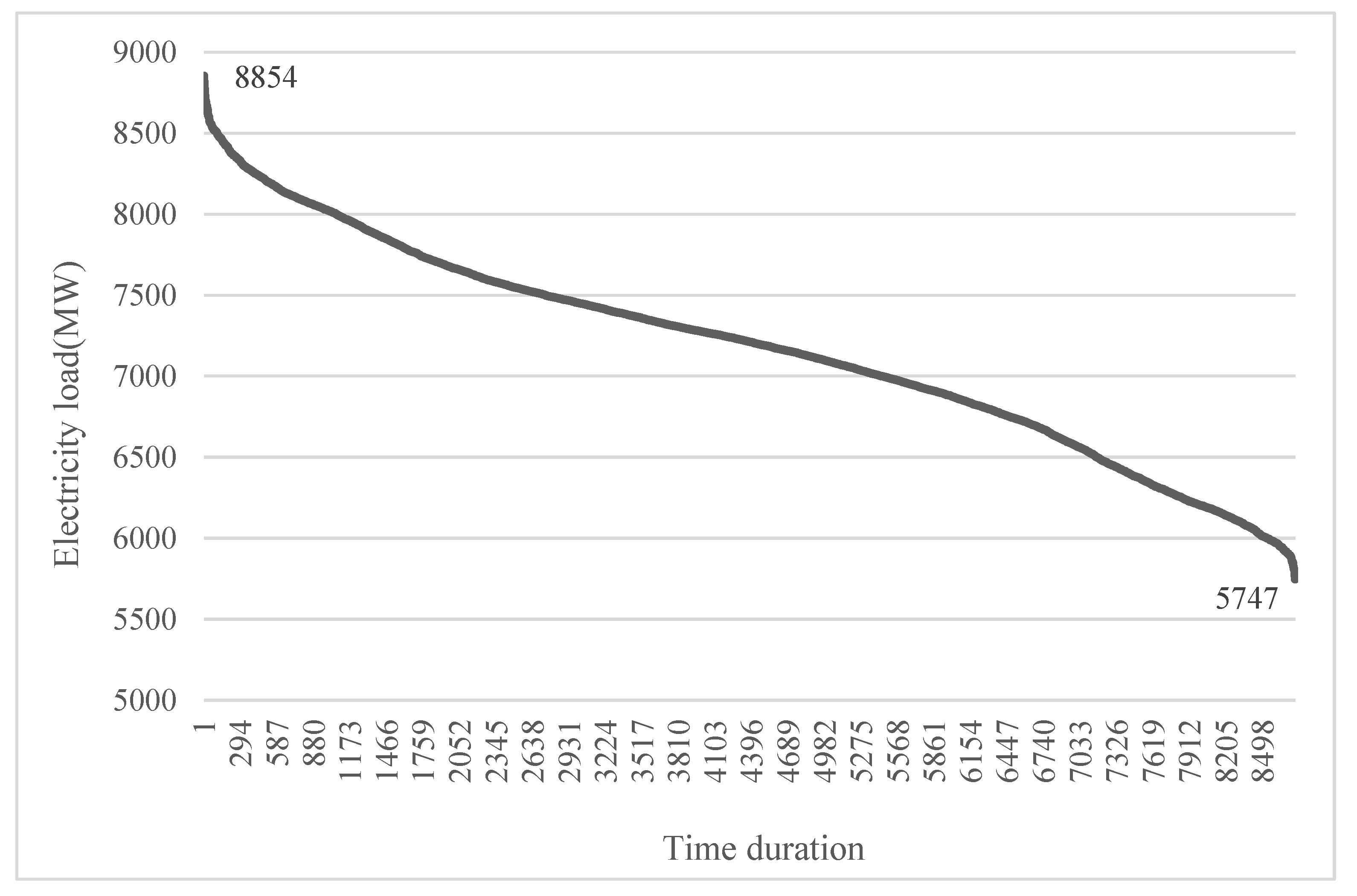
Electricity demand in Alberta has increased over the past several years, although load has remained relatively stable within a given year because more than half of the demand comes from industrial and commercial activities. Specifically, about one-third of the total Alberta internal load (AIL) is from the industrial sector; one-fifth comes from commercial activities and the remainder is contributed by residential and farm customers [4]. A load duration curve rearranges the hourly load (demand) throughout a year from highest to lowest, with the lowest load to be met by baseload generators—thermal assets, such as coal, nuclear or combined-cycle gas turbines (CCGT), or a hydroelectric facility with reservoir. For our modelling, we estimate hourly demand by adding up hourly generation from different assets and net imports. The available hourly data on AIL are on average greater than our estimated hourly supply by adding up generation by different assets, including net imports. We consider this difference to be primarily driven by behind the fence load and industrial self-generation. Alberta’s load duration curve for 2019 is provided in Figure 3; the highest load is 8854 MW, while the baseload is 5747 MW. In our study, we ignore any generation used to self-supply behind-the-fence load and consider only the system load that is external to the generating assets [33]. The Alberta internal load represents the system load plus load served by on-site generating units, including those within an industrial system and the City of Medicine Hat.

In Alberta, electricity is generated from multiple sources.

Table 1. Alberta Electric System Generating Capacity in 2019 (MW).

Year	Coal	Cogen a	CCGT Gas b	OCGT Gas c	Hydro	Wind	Other	Total
2019	5723	5043	1748	905	894	1781	438	16,532

^a Cogen refers to cogeneration which is used primarily in industrial plants. ^b Combined-cycle gas turbine (CCGT) provides baseload power. ^c Open-cycle gas turbine (OCGT) refers to fast-responding (peak load) gas turbines. Source: AESO [36].

shows the composition of Alberta’s generating capacity in 2019. These capacity data are used as the base case scenario for calibration purposes. Thermal generators still dominate the mix, with coal and gas accounting for 80% of total system capacity; as a result, there is great potential to introduce more renewable electricity generation ([34,35]). In 2019, several coal-fired facilities were converted to co-fire with natural gas. The AESO was unable to discern which fuel was being utilized at any given time, so data related to coal-fired generation may reflect natural gas firing at these facilities. During 2021, five coal assets were converted to fire natural gas. In 2019, Alberta did not rely on utility-scale battery storage, but, by 2021 two new battery storage stations had been built along with wind farms [31].

Cost information is from the AESO, U.S. Energy Information Administration (EIA), and various other sources, as indicated in

Table 2. Cost of Electricity Estimates for OCGT, CCGT, Solar, Wind and Battery Power (CAD 2019 per MWh) ^a.

Type	Overnight Capital Cost (CAD/kW)	Fixed O & M (CAD/kW/yr)	Fuel Cost (CAD/MWh)	Variable O & M (CAD/MWh)	Emissions (tCO2/MWh)	Facility Life (Years)
Coal		53	21.6	5.9	0.63
OCGT	1159	57.3	16.5	4.6	0.17	25
CCGT	1667	53.9	11.9	2.7	0.023	30
Cogeneration		53.9	23.6	2.7	0.022
Biomass	2501	164.3	56.5	6.31	0.965
Run of River		54.6	2.56	13.62	0.024
Brazeau and Bighorn Reservoirs		54.6	2.56	13.62	0.024
Solar	1643	19.9	0	0	0.048	25
Wind	1586	32.5	0	0	0.012	25
Li-ion battery	1515	32.4	0	0	0.3	10

^a Authors’ calculations based on data from AESO ([28,34]), EIA [38], Rapier [39], Schlömer et al. [40] and Sönnichsen [41]. O & M stands for operations and maintenance cost.

. All monetary values are converted to Canadian dollars. In recent years, the cost of renewables fell significantly [37]. We use scenario analysis to investigate how the Alberta electricity generation mix responds to different assumptions about costs. For example, we simulate changes in the generation mix resulting from changes in carbon taxes and the imposition of emission standards.

Alberta has excellent potential to deploy renewable resources to generate electricity for two reasons. First, Alberta has abundant wind and solar resources, with wind power especially high during winter and in June, while solar output is high in summer but low in winter [42]. During the day, solar power is highest at noon and wind power is at its peak at night. In essence, wind and solar power are complementary, but solar power is more valuable than wind power because solar is available at a time when demand and prices are greatest. A second reason why Alberta is a good place to invest in renewables relates to its electricity market, which is deregulated so electricity companies can make asset investment decisions independently. Thus, the market is quite resilient to economic shocks and responsive to policy incentives, such as carbon taxes.

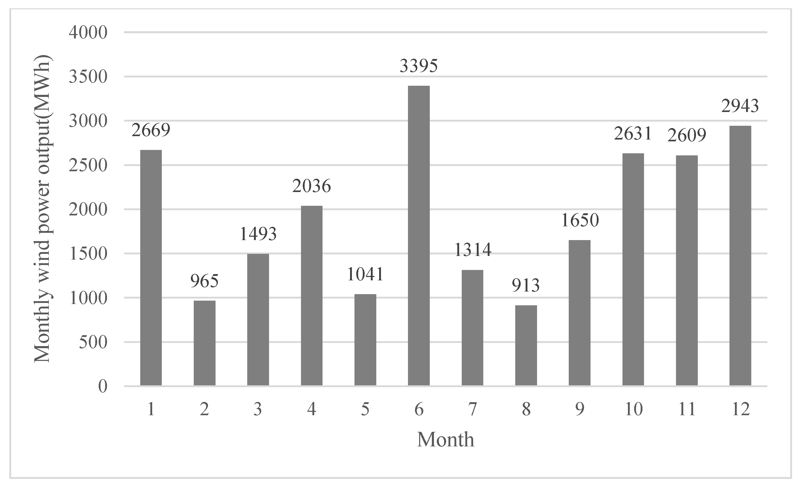
To estimate potential generation capacity from wind and solar, we modelled two representative generators [43]. We used the 2019 wind speed profile for Pincher Creek from Environment and Climate Change Canada [44] and an ENERCON E-126 7.58 MW wind turbine to estimate electricity output (see Figure 4). Conversion of the available mechanical energy (wind speed) to electricity is based on technical specifications. Wind generation was stronger in 2020 than in 2019, resulting in an increase in the average capacity factor from 30% to 39%; the capacity factor was also 15–20% higher in winter than in summer [36]. In our simulations, the average annual capacity factors are around 35%.

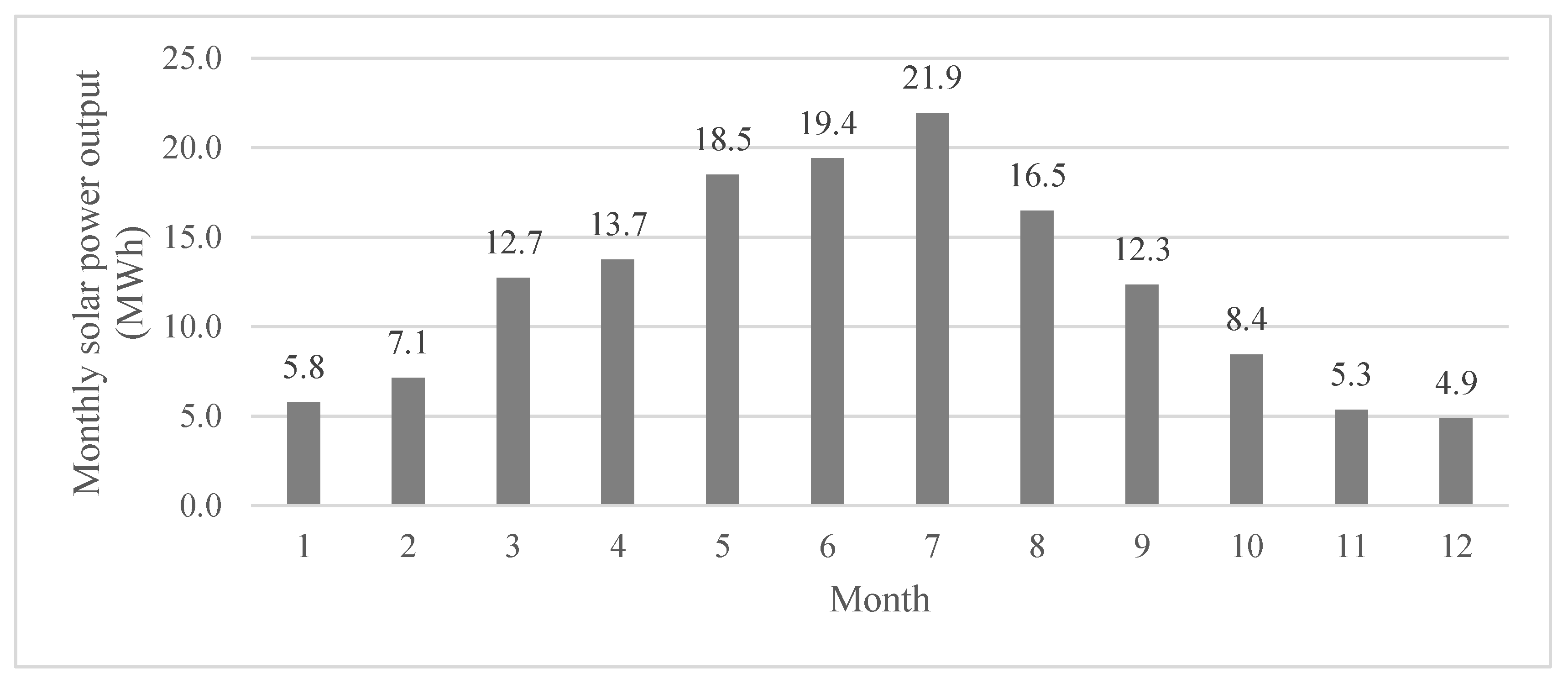
In addition to high wind profiles, southern Alberta has one of Canada’s highest solar potentials, which explains why one of the largest solar farms in North America was developed in Vulcan County in 2021 [45]. We used solar radiation and temperature information for Pincher Creek in 2017 from Canadian Weather Energy and Engineering Datasets ([44,45]) and a Canadian Solar CS6X_300P panel to calculate potential solar power output (see Figure 5). The Canadian Weather Energy and Engineering Datasets (CWEEDS) provides annual data on a range of meteorological elements, recorded hourly at a grid spacing of about 10 × 10 km grid. The solar energy outputs were calculated using the PVLIB package in Python, developed by Sandia National Laboratories [46].

3.2. Calibrating Cost Functions for Alberta Electricity Generation

Using the quadratic cost functions in Equation (21), we can recover observed generation for the Alberta grid in 2019 by asset types. The differences between model solutions and observed generation are summarized in

Table 3. Differences between Calibrated and Observed Outputs for Four Generator Types, based on the Second Calibration Method.

	Coal	Open-Cycle Gas Turbine (OCGT)	Combined-Cycle Gas Turbine (CCGT)	Brazeau and Bighorn Reservoir
RMSE a	4.018	0.121	0.189	0.103
MAE b	0.496	0.116	0.130	0.103
MAPE c	0.000	0.000	0.000	0.002

^a Root mean squared error. ^b Mean absolute error. ^c Mean absolute percent error.

using the second identification strategy [S2] in Equation (25). The calibrated cost functions not only capture the explicit accounting costs but also the implicit economic costs as they replicate observed generation. The implicit economic costs could come from capacity constraints or ramping up/down constraints, et cetera.

To study the sensitivity of our results, we calibrate the model using data the years 2014 through 2020. The sensitivity analysis revealed that the calibration algorithm does not necessarily converge for all years due to dual degeneracy or other numerical issues. In the context of the Alberta model, PMP yielded successful convergence of the calibration parameters for the years 2017 and 2019. Subsequently, we discuss the simulation results with 2019 as our base case, although the simulation results using 2017 data are similar in terms of long-run patterns but with differences in short-run patterns. The differences between actual hourly generation and recovered generation using calibrated costs never exceed 0.1 percent. Nonetheless, calibrated marginal costs can vary between the two years as summarized in

Table 4. Calibrated Marginal Costs (CAD/MWh).

Generator Type		2017	2019
Coal	Mean	29.29	55.13
	Median	27.50	33.51
	Std Dev	26.08	90.30
	25th percentile	27.50	31.42
	75th percentile	27.50	45.17
	95th percentile	32.52	101.71
OCGT	Mean	29.28	55.13
	Median	27.49	33.51
	Std Dev	26.08	90.29
	25th percentile	27.47	31.42
	75th percentile	27.50	45.17
	95th percentile	32.52	101.70
CCGT	Mean	29.29	55.13
	Median	27.50	33.51
	Std Dev	26.08	90.30
	25th percentile	27.50	31.42
	75th percentile	27.50	45.17
	95th percentile	32.52	101.70
Hydraulics: Brazeau and Bighorn	Mean	29.28	55.09
	Median	27.49	33.49
	Std Dev	26.07	90.24
	25th percentile	27.48	31.39
	75th percentile	27.49	45.14
	95th percentile	32.51	101.62

Source: Authors’ calculations.

.

3.3. Power Generation Mix Optimization with Calibrated Cost Function

Once the grid optimization model is calibrated, we simulate the impacts of various climate policies on the electricity generation mix. In doing so, we allow the system operator to remove fossil-fuel power plants and add renewable power assets along with battery storage. However, since electricity prices are not known at this stage (they are used only in calibrating the parameters of the cost functions), a cost minimization problem now needs to be specified—the system operator must satisfy the electricity demand and all technical constraints at minimum cost. The system operator specifically minimizes the following total cost function:

$$Z_{\mathrm{AB}}={{\displaystyle \sum }}_{\mathrm{t}=1}^{\mathrm{T}}\left\{\begin{array}{c}{\displaystyle \sum }_{\mathrm{f}}\left({\mathrm{d}}_{\mathrm{f},\mathrm{t}}+\frac{1}{2}{\mathrm{q}}_{\mathrm{f},\mathrm{t}}{G}_{\mathrm{f},\mathrm{t}}\right)G_{\mathrm{f},\mathrm{t}}+\\ {\displaystyle \sum }_{\mathrm{r}}{\mathrm{c}}_{\mathrm{r}}{G}_{\mathrm{r},\mathrm{t}}+\\ {\displaystyle \sum }_{\mathrm{i}=1}^{\mathrm{I}}\left[\left({\mathrm{c}}_{\mathrm{i}}^{\mathrm{on}}+{\mathrm{c}}_{\mathrm{i}}^{\mathrm{fom}}\right)K_{\mathrm{i}}^{+}+{\mathrm{c}}_{\mathrm{i}}^{\mathrm{fom}}\left({\mathrm{K}}_{\mathrm{i}}-K_{\mathrm{i}}^{-}\right)\right]+\\ \tau {\displaystyle \sum }_{\mathrm{i}}{\mathrm{E}}_{\mathrm{i}}{G}_{\mathrm{i},\mathrm{t}}\end{array}\right\},$$

(27)

where f refers to coal, open-cycle gas (OCGT), combined-cycle gas (CCGT), and the Brazeau-Bighorn hydroelectric facility that has storage reservoirs; r refers to wind, solar, battery storage, and other non-dispatchable assets; i refers to all generating assets; ${\mathrm{c}}_{\mathrm{i}}^{\mathrm{on}}$ represents the annualized overnight cost of electricity (CAD/MWh); ${\mathrm{c}}_{\mathrm{i}}^{\mathrm{fom}}$ is the fixed operation and maintenance cost (CAD/MWh); ${\mathrm{K}}_{\mathrm{i}}$ refers to existing generating capacity (MW); $K_{\mathrm{i}}^{+}$ is added capacity (MW); $K_{\mathrm{i}}^{-}$ is capacity that is removed (MW); ${\mathrm{E}}_{\mathrm{i}}$ refers to CO₂ emissions (tCO₂/MWh) from generation type i; and $\mathsf{\tau }$ is the carbon tax (CAD/tCO₂).

Equation (27) is minimized subject to demand (Equation (16)) and other technical constraints (e.g., ramping constraints). To study the effects of policies on generation and asset capacities, the model allows the system operator to change the fossil fuel and renewable capacities so that the system could achieve proactively the CO₂ emission reduction goals. Therefore, the capacity constraints (15) change accordingly.

For the base case and ensuing simulations, we use the 2019 hourly loads to solve for the optimal generation mix. The carbon tax in Alberta was CAD 30/tCO₂ in 2019, so our calibrated costs for the base year take into account the extant carbon tax. We then solve the model using the calibrated quadratic cost functions. The model does not add any renewable power capacity to the system. Instead, as a means of minimizing cost, it removes around 15% of the existing capacity of CCGT, 26% of OCGT, and 24% of coal in the base case scenario. Since we assume that the existing asset investments in the grid are optimal, we consider these removed capacities as reserves necessary for avoiding outages. Additionally, the model solutions are static in the sense that, given the hourly base-year loads, it minimizes cost by choosing the generators and their output—no account is taken of future expectations or forecasted demand growth. Hence, in the subsequent policy analysis sections, any fossil fuel capacities removed (or added) beyond the base case are treated as potential removals (or additions). A summary of the base-case results is found in

Table 5. Generation and Emissions in the base case.

	Total Generation (TWh)	Total Emission (Mt)
Base Case (2019)	62.89	19.33
	Share of Total Generation (%)	Share of Total Emission (%)
Biomass	1%	3.1%
Coal	44%	90.4%
OCGT	6%	3.2%
Cogeneration	22%	1.6%
CCGT	15%	1.1%
Brazeau and Bighorn	1%	0.1%
Run of River	2%	0.1%
Solar	<0.1%	<0.1%
Wind	9%	0.3%
Battery Storage	0%	0%

Source: Authors’ calculations.

.

The main policy instruments in our analysis are a carbon tax and an emissions standard. Under the carbon tax, we first solve the model imposing an increasing carbon tax up to CAD 200/tCO₂ using the current cost level (Section 3.4) and then examine the impacts of emission standards (Section 3.5).

3.4. Carbon Tax Scenarios

It is evident that, with a rising carbon tax, the optimal solution reduces fossil-fuel capacities and increases renewable energy sources in the generation mix. One aspect worth considering, however, is how these assets displace one another in the process.

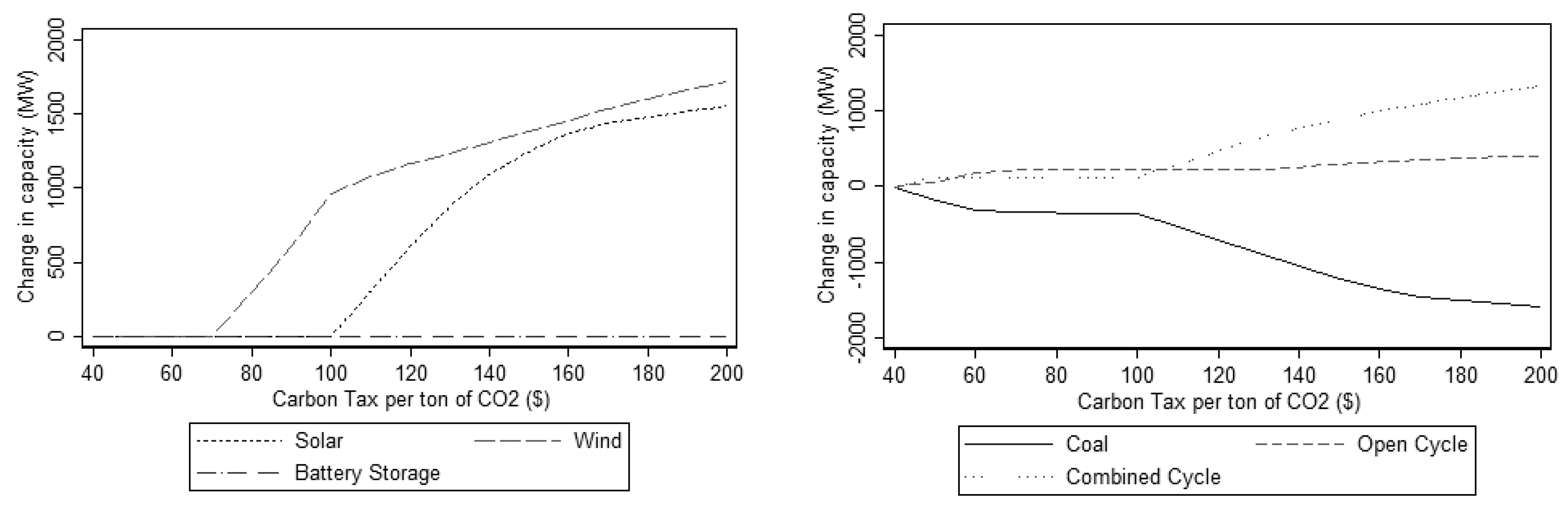
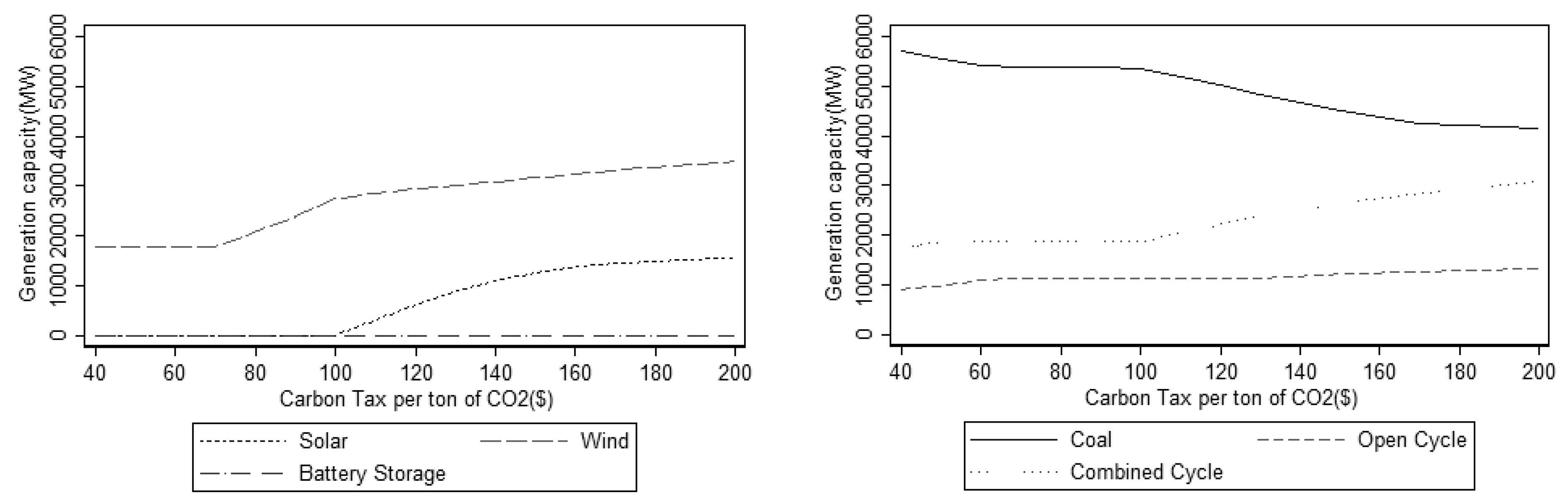
Figure 6 presents the changes in asset capacities that occur as the carbon tax increases, while Figure 7 provides total capacities. There is a high correlation between changes in coal capacity and changes in CCGT capacity; when coal capacity falls, CCGT capacity increases, and when coal capacity is unchanged so is CCGT capacity. Surprisingly, there is no correlation between changes in coal capacity and changes in the capacities of renewable energy sources—when the capacity of renewables increases, coal capacity does not decrease correspondingly. However, there is competition between renewables—when solar capacity increases, the investment in wind assets slows down. When the carbon tax increases to around CAD 65/tCO₂, coal capacity declines rapidly, while OCGT and CCGT capacities increase slightly. Tax rates between CAD 65/tCO₂ and CAD 130/tCO₂ have little impact on optimal capacities of fossil-fuel generators, but, when the tax rate exceeds CAD 130/ tCO₂, coal capacity declines further while there is an increase in CCGT capacity—baseload gas capacity replaces baseload coal capacity. At the same time, there is hardly any change in OCGT capacity. Although peak-load OCGT is used to meet rapid changes in load due to intermittent wind, say, reliance on OCGT is more expensive than CCGT. Yet it is surprising that the model does not add more peak OCGT capacity, although CCGT assets ramp up and down somewhat faster than coal assets.

Finally, wind power capacity increases sharply when tax rates are between CAD 90/tCO₂ and CAD 130/tCO₂. When the carbon tax reaches CAD 130/tCO₂, new solar capacity is added to the system, while reliance on wind energy slows down. However, additional wind and solar capacities are not able to replace baseload or peak load gas capacity. In terms of capacity substitution, additional wind and solar capacities do not have much impact. When the carbon tax reaches CAD 200/tCO₂, wind capacity reaches 3617 MW and solar capacity 1652 MW. The amount of renewable capacity added to the system is much greater than the reduction in coal capacity.

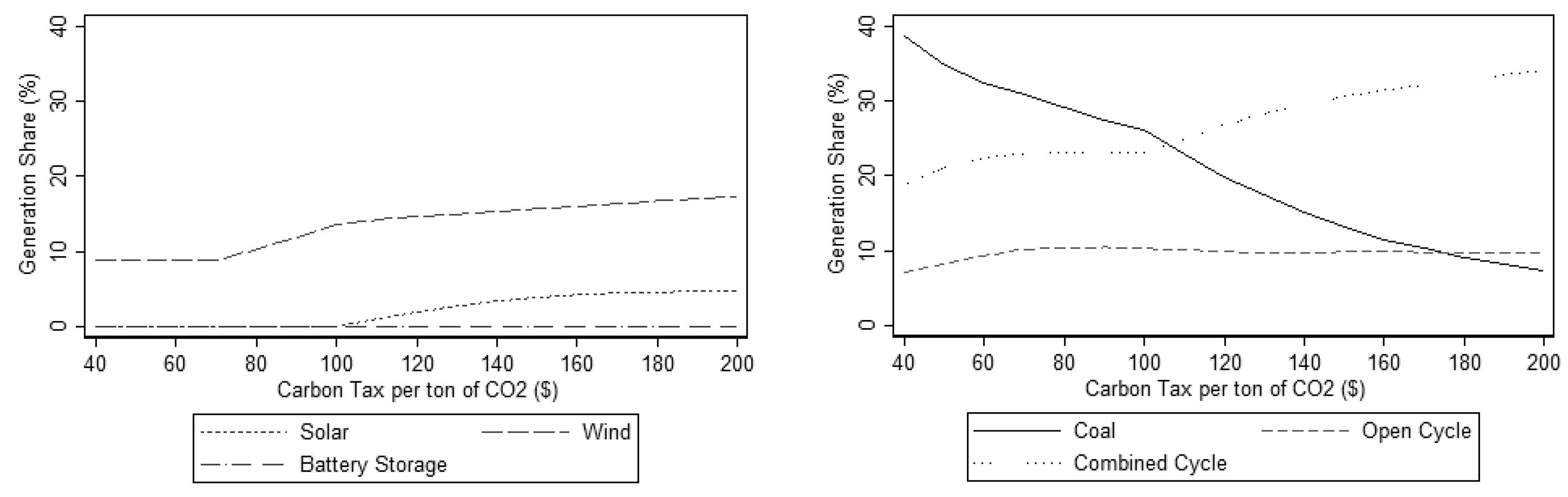
If we consider the impact of renewables on total generation, we find that renewables play a vital role in substituting for fossil-fuel generation (Figure 8). Starting from 9% in the base case, the total generation share of renewables reaches around 23% (18% from wind, 5% from solar) when the carbon tax is CAD 230/tCO₂. Some 1600 MW of solar capacity is added to the base solar capacity of 15 MW, which is about half of the total wind capacity; nonetheless, the generation share of solar power is only one-third that of wind, which implies that the capacity factor of solar is lower than that of wind power. Further, the share of the generation coming from coal declines from 42% (base case) to 7% (CAD 200/tCO₂ tax), but importantly, the generation share of CCGT increases from 16% to 35%. Overall, less than half of the lost generation share from coal is replaced by renewables, with more than half replaced by CCGT.

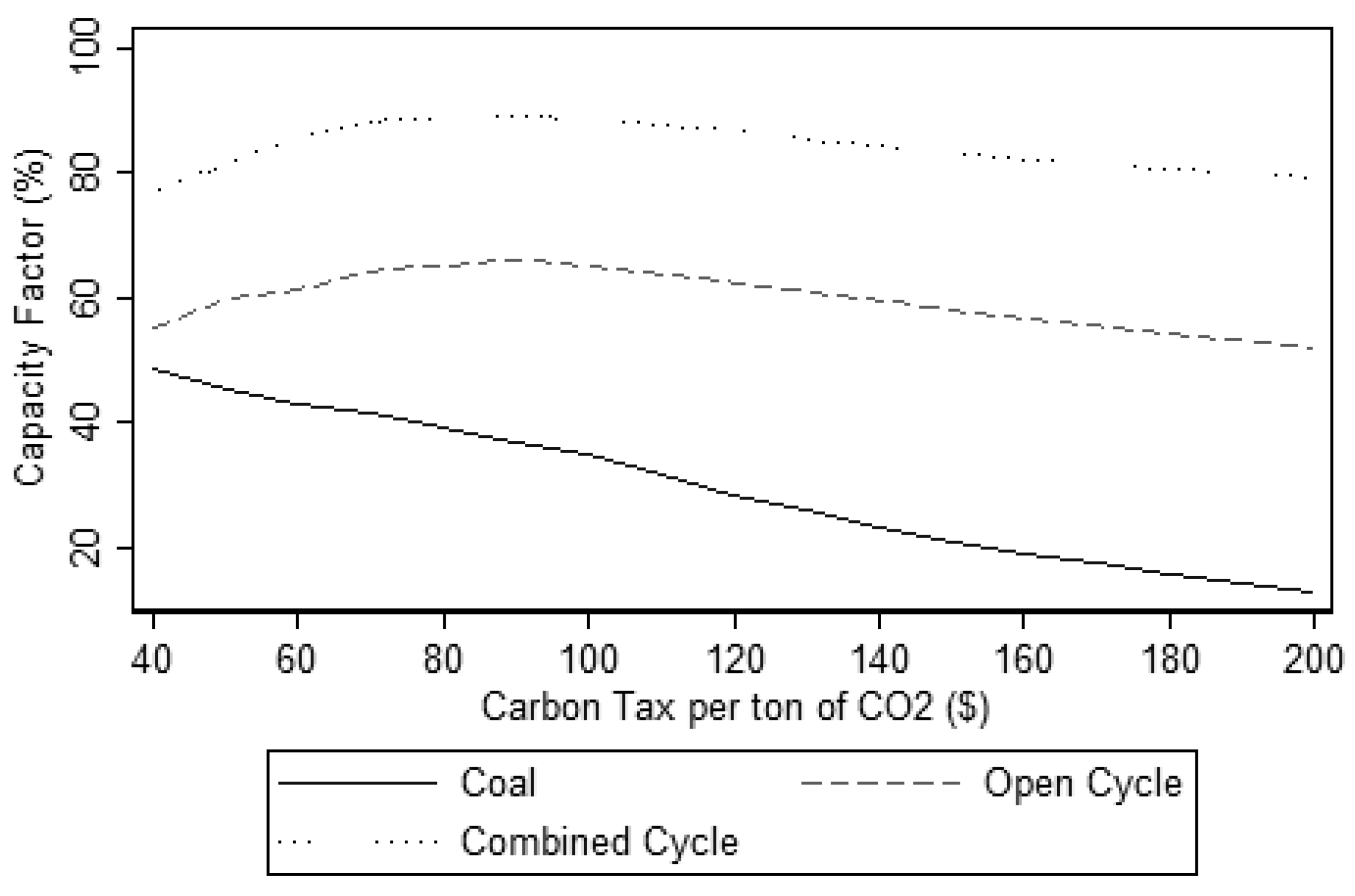
The capacity factor (CF) is determined as actual generation over a period divided by potential generation. For example, a 100-MW capacity generator has the potential to produce 876,000 MWh of energy over a year (=8760 h × 100 MW); if it produced 450,000 MWh over some year, its CF is 51.4% (=450/876). The CF helps us understand the interaction between fossil fuels and renewables (Figure 6 and Figure 7). In Alberta, the CF for coal generation fell from 80% to 60% in the years before 2020, while the CF of CCGT has continued at about 70% [33].

Results in Figure 9 are similar. First, the CF for coal continues to decline from 54% to 11% as coal generation decreases faster than the reduction in coal-fired capacity. When we have abundant renewables, coal-fired power is not needed, but a large amount of coal capacity is still required as backup capacity. Newly added renewable capacity replaces some coal generation, but it has less impact on reducing coal capacity. Second, the CFs of OCGT and CCGT initially increase, but when new wind and solar power are added, the CFs slowly decline. More renewable capacity and generation lead to less efficient OCGT and CCGT power use.

The CFs for wind and solar power in our model are decided by the natural wind and solar resources, which do not change when the carbon tax increases. However, the CF of a storage device does fall from 33% to 16%, but there is too little storage to decide whether this result is applicable under different conditions.

Our findings are solid when it comes to the price of renewable energy. We also run simulations for scenarios where the cost of renewable energy assets is cut in half from the baseline level. The results from the simulation match those from this section.

3.5. Clean Electricity Emission Standards

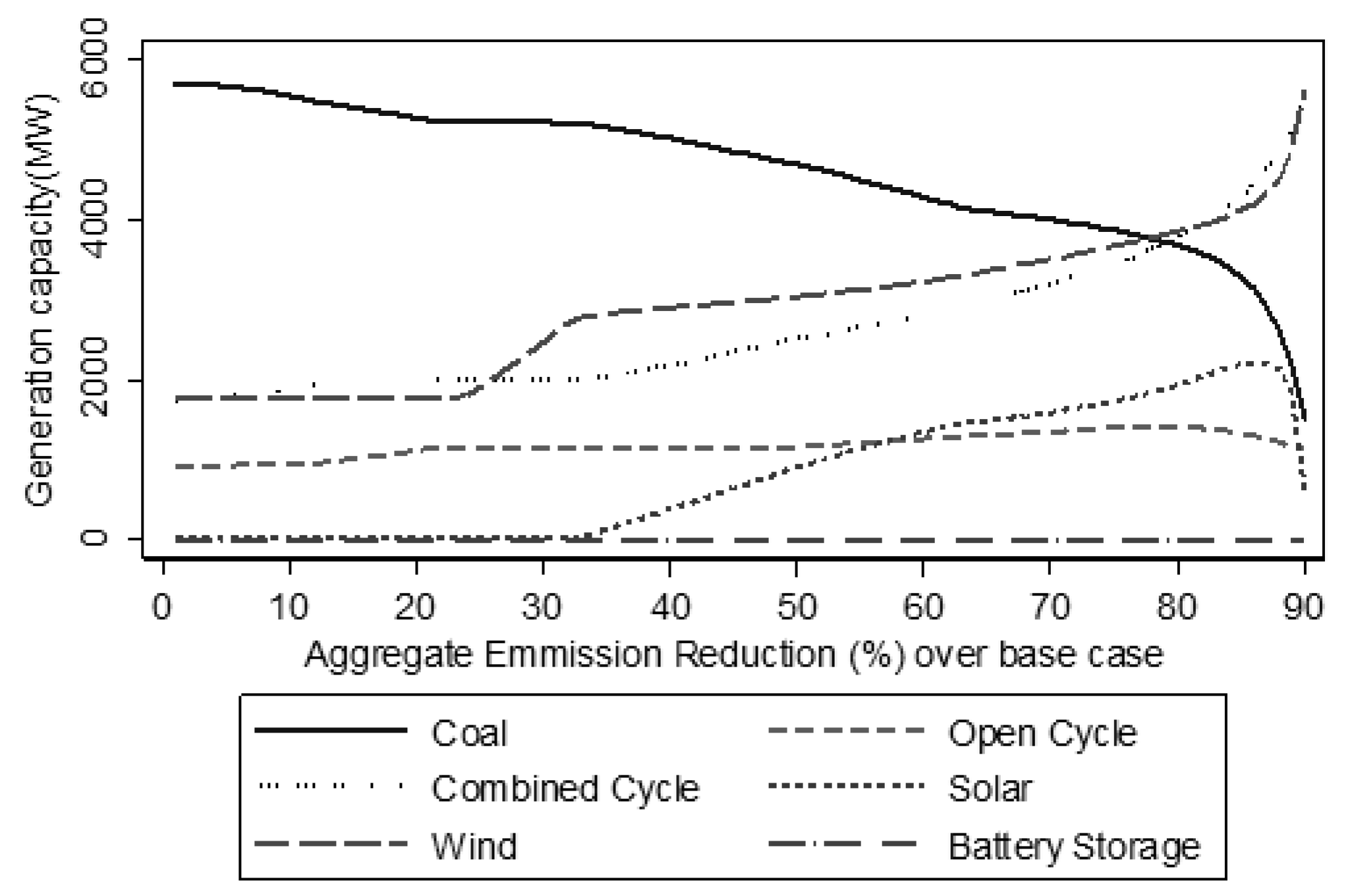
An alternative policy instrument is to implement emission standards. To investigate the impacts of clean electricity standards on the generation mix, we introduce emission reduction requirements as an additional constraint in the model, while imposing no carbon tax and keeping renewable costs at the base level. With an increased carbon emission reduction target, we expect to see a reduction in fossil-fuel generation capacities and an increase in renewable capacities. When the emission reduction target reaches 85% compared to the base case, optimal solar power capacity falls while wind and CCGT capacities rise sharply (Figure 10). When the target increases to 90%, solar power is even driven out of the generation mix, and the share of coal power in the generation mix steadily declines toward zero. The reason is that the lifetime emissions from solar power are higher than from wind due to the construction of solar panels. Hence, the simulation results show that, in the extreme situation, we choose wind over solar to reduce carbon emissions.

With an 85% emissions-reduction target, the total capacity of wind and CCGT is 11,256 MW, which is much higher than peak demand (8854 MW). At the same time, OCGT capacity remains quite high. The results show that, to backstop intermittent renewables when the emission reduction standard is high, overinvestment in CCGT, OCGT, and renewable capacities is unavoidable, which might lead to economic inefficiency and further reinforce the missing money problem. With a 90% emission-reduction target, total capacity rises to 14,570 MW, and the total capacity for wind and CCGT assets remains at 11,256 MW.

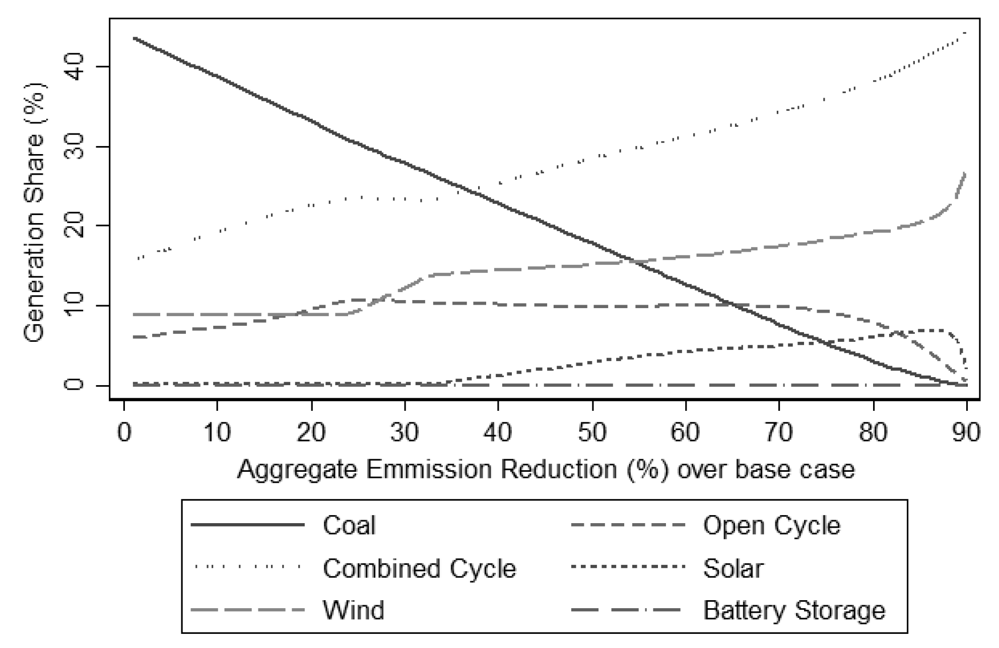
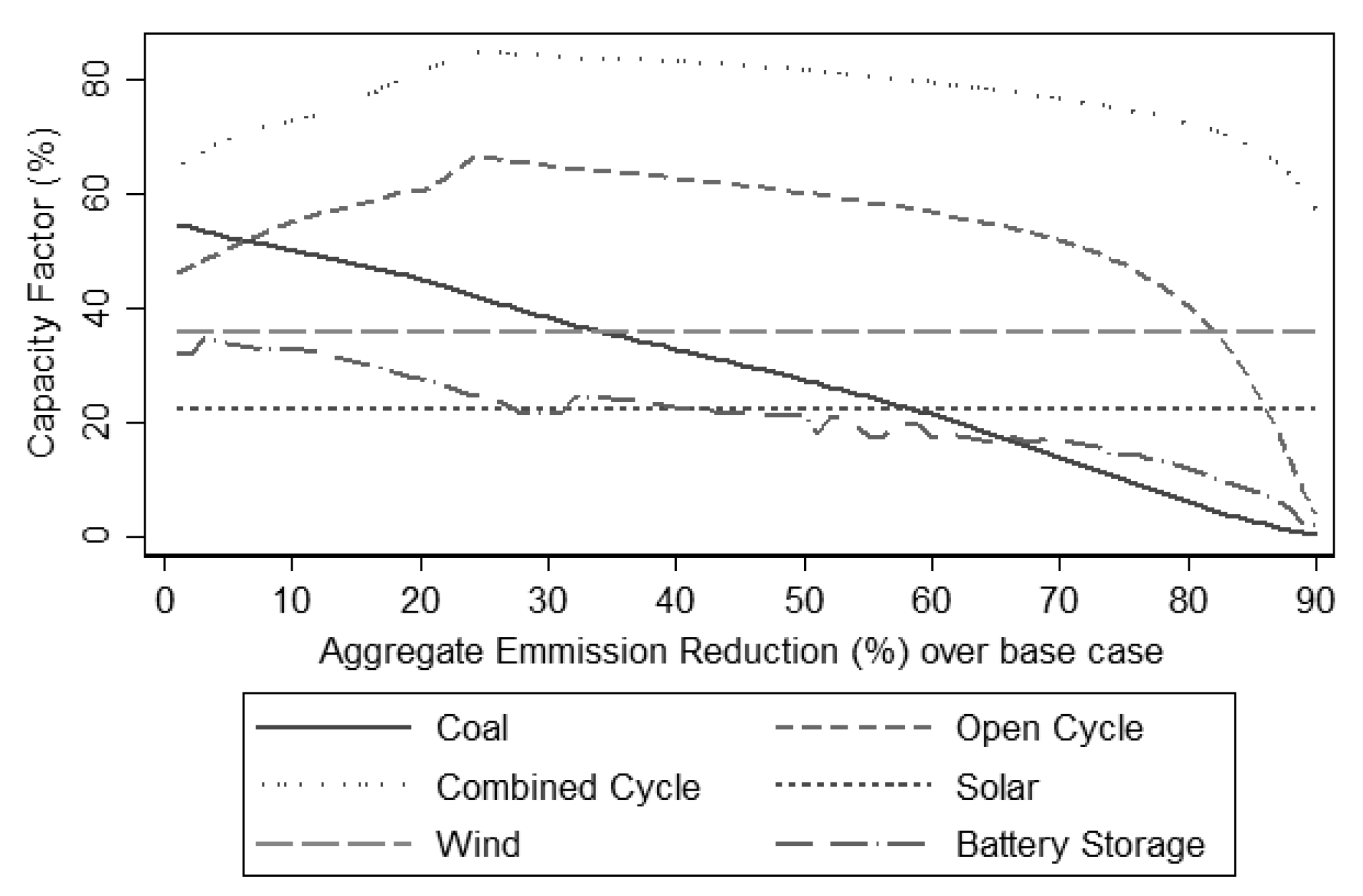
The changes in generation shares (Figure 11) and capacity factors (Figure 12) reflect a similar situation. CCGT and wind power production dominate electricity supply. Despite a high capacity, the generation share of OCGT declines rapidly when the reduction target reaches 70%; the CF begins to decline as early as an emissions-reduction target of 25%. The CFs for coal and battery storage steadily decrease with an increasingly stringent carbon emissions reduction target.

Overall, the simulation results here indicate that renewables generation could replace coal generation, but wind and solar power cannot be used as reliable baseload assets, requiring instead a large degree of CC gas capacity and generation. Further, the capacity factors of thermal generators fall because they are relied upon to generate power less often resulting in inefficient resource allocation. To improve the efficacy while meeting the carbon emission reduction goal, the electricity industry needs some reliable and less carbon-intensive alternatives to provide necessary baseload capacity. For example, many developing countries such as China and India have turned to nuclear power, with some developed countries, such as France and the Netherlands, also planning to build more nuclear power plants [47,48]).

4. Conclusions and Policy Implications

A growing share of intermittent renewables in electricity grids adds complexity to an already intricate system, creating greater challenges for grid operators and policymakers. Models of electricity grids can be an important tool to help decision makers, perhaps enabling them to avoid blackouts such as the one that affected the Western Interconnection in 1996 [49] and California in 2020–2021 [50]. While off-the-shelf engineering models are useful for operational purposes [43], they lack the scope to study longer-term policy effects. In this paper, we proposed a grid model using a calibration method that enables the researcher to parameterize upward-sloping marginal cost functions for modelling electricity grids—essentially calibrating screening curves for fossil-fuel generation. Based on a screening-curve-load-duration method, it allowed us to study optimal generation mixes based on various policy parameters and potential wind/solar regimes. Our study employed a simple yet effective way to analyze policy scenarios with reasonably minimal data on the electricity wholesale market, thereby providing a novel contribution to the calibration literature as it pertains to electricity grid models.

Using this approach, we examined several climate policies to determine how renewable wind and solar generating assets would optimally enter an electricity grid (Alberta) dominated by fossil-fuel assets. The calibrated upward-sloping supply functions provided a realistic allocation of load across assets, tracing out the effect of a carbon tax or emission standard on the grid. For example, rather than coal power suddenly disappearing from the generation mix when there is a small change in the carbon tax, a smooth phasing out process may be optimal (viz., slow increase in a carbon tax), thereby avoiding disruptive and costly shutdowns and start-ups (as in Europe in 2023 as a result of reduced availability of natural gas) [51].

We analyzed the impact of two policy scenarios—a carbon tax and an emissions reduction target. Not surprisingly, the capacities and generation shares of renewables increase, and those of coal-fired power decrease, under both an increasing carbon tax and an emission reduction target. The capacity and generation of natural gas assets on the other hand rise, while their capacity factors fall. Because OCGT and CCGT replace coal to provide reliable baseload and peaking generation, their optimal capacities remain high, but their use decreases as more electricity is produced by renewables. Overall, wind and solar power are unreliable and unsuitable for meeting continuous baseload and peaking load requirements. Consequently, significant natural gas generating capacity is required to backstop intermittent generation, although gas power output is required less frequently, leading to lower capacity factors and loss of quasi-rents (the “missing money”) required to incentivize investments in gas plants. To rectify this capacity, payments are needed, but these raise retail electricity prices [52].

The policy findings based on a calibrated model of the Alberta electricity grid are also relevant for other regions. Observations with regards to the missing money problem and capacity payments for investments in backup assets have already been noted in the context of the UK and EU [53]. Analogous policy implications have been found as well for Australia, where gas is competitive with coal but, unlike coal, complements the uptake of renewables [54].

Finally, the calibration method proposed in this paper can be used to study a variety of other policy issues, including the impact of changes in the cost of building new plants, changes in hourly demand, and changes in the water inflow of hydroelectric dams on overall generation and capacity mixes. One interesting extension to our approach would be to calibrate transmission costs across multiple regions and create a model that allows for imports and exports while satisfying each region’s load. However, other calibration methods will also need to be investigated.

References

- Brouwer, K.M.; Bergkamp, L. Road to EU Climate Neutrality by 2050. Spatial Requirements of Wind/Solar and Nuclear Energy and Their Respective Costs; ECR Group and Renew Europe, European Parliament: Brussels, Belgium, 2021. [Google Scholar]
- Lund, H. Large-scale integration of wind power into different energy systems. Energy 2005, 30, 2402–2412. [Google Scholar] [CrossRef]
- van Kooten, G.C. The economics of wind power. Annu. Rev. Resour. Econ. 2016, 8, 181–205. [Google Scholar] [CrossRef]
- van Kooten, G.C.; Mokhtarzadeh, F. Optimal investment in electric generating capacity under climate policy. J. Environ. Manag. 2019, 232, 66–72. [Google Scholar] [CrossRef] [PubMed]
- Stahel, A. The Crisis of the European Energy System; vol. GWPF Note 35; Global Warming Policy Foundation: London, UK, 2022. [Google Scholar]
- van Kooten, G.C. All You Want to Know About the Economics of Wind Power; University of Victoria: Victoria, BC, Canada, 2015. [Google Scholar]
- International Energy Agency (IEA). Electricity Market Report, July 2021; International Energy Agency (IEA): Paris, France, 2021. [Google Scholar]
- PA Media. Energy Crisis Could Halt Factory Production, Industry Leaders Warn | Energy Industry | The Guardian. 2021. Available online: https://www.theguardian.com/business/2021/oct/08/energy-crisis-could-halt-factory-lines-industry-leaders-warn (accessed on 19 July 2022).
- Barrett and Philip. How Food and Energy are Driving the Global Inflation Surge. International Monetary Fund. Available online: https://www.imf.org/en/Blogs/Articles/2022/09/09/cotw-how-food-and-energy-are-driving-the-global-inflation-surge (accessed on 12 January 2023).
- Jenkins, J.; Sepulveda, N. Enhanced Decision Support for a Changing Electricity Landscape: The GenX Configurable Electricity Resource Capacity Expansion Model; MIT: Cambridge, MA, USA, 2017. [Google Scholar]
- Howells, M.; Rogner, H.; Strachan, N.; Heaps, C.; Huntington, H.; Kypreos, S.; Hughes, A.; Silveira, S.; DeCarolis, J.; Bazillian, M.; et al. OSeMOSYS: The Open Source Energy Modeling System: An introduction to its ethos, structure and development. Energy Policy 2011, 39, 5850–5870. [Google Scholar] [CrossRef]
- Foley, A.M.; Gallachóir, B.P.; Hur, J.; Baldick, R.; McKeogh, E.J. A strategic review of electricity systems models. Energy 2010, 35, 4522–4530. [Google Scholar] [CrossRef]
- Streitberger, C. On the Economics of Renewable Energy Support and Market Integration of Intermittent Electricity Supply. Ph.D Thesis, ETH Zurich, Zurich, Switzerland, 2020. [Google Scholar]
- Joskow, P.L. Competitive Electricity Markets and Investment in New Generating Capacity; Elsevier: Amsterdam, The Netherlands, 2006. [Google Scholar]
- Prescott, R.; van Kooten, G.C. Economic costs of managing of an electricity grid with increasing wind power penetration. Clim. Policy 2009, 9, 155–168. [Google Scholar] [CrossRef]
- Ahmed, T. Modeling the Renewable Energy Transition in Canada; Springer: Berlin/Heidelberg, Germany, 2016. [Google Scholar]
- Paris, Q. Economic Foundations of Symmetric Programming; Cambridge University Press: Cambridge, MA, USA, 2010. [Google Scholar]
- Karnon, J.; Vanni, T. Calibrating Models in Economic Evaluation. Pharmacoeconomics 2011, 29, 51–62. [Google Scholar] [CrossRef]
- Howitt, R.E. Positive Mathematical Programming. Am. J. Agric. Econ. 1995, 77, 329–342. [Google Scholar] [CrossRef]
- Heckelei, T. Calibration and Estimation of Programming Models for Agricultural Supply Analysis. Ph.D Thesis, Universität Bonn, Bonn, Germany, 2002. [Google Scholar]
- Röhm, O.; Dabbert, S. Integrating Agri-Environmental Programs into Regional Production Models: An Extension of Positive Mathematical Programming. Am. J. Agric. Econ. 2003, 85, 254–265. [Google Scholar] [CrossRef]
- Liu, X.; van Kooten, G.C.; Duan, J. Calibration of agricultural risk programming models using positive mathematical programming. Aust. J. Agric. Resour. Econ. 2020, 64, 795–817. [Google Scholar] [CrossRef] [Green Version]
- De Frahan, B.H.; Buysse, J.; Polomé, P.; Fernagut, B.; Harmignie, O.; Lauwers, L.; van Huylenbroeck, G.; van Meense, J. Positive mathematical programming for agricultural and environmental policy analysis: Review and practice. Int. Ser. Oper. Res. Manag. Sci. 2016, 99, 129–154. [Google Scholar]
- Heckelei, T.; Britz, W.; Zhang, Y. Positive mathematical programming approaches–recent developments in literature and applied modelling. Bio-Based Appl. Econ. J. 2012, 1, 109–124. [Google Scholar]
- Johnston, C.M.T.; van Kooten, G.C. Impact of inefficient quota allocation under the Canada-U.S. softwood lumber dispute: A calibrated mixed complementarity approach. For. Policy Econ. 2017, 74, 71–80. [Google Scholar] [CrossRef]
- Howitt, R. Agricultural and Environmental Policy Models: Calibration, Estimation and Optimization; University of California: Davis, CA, USA, 2005. [Google Scholar]
- Paris, Q.; Howitt, R.E. An Analysis of Ill-Posed Production Problems Using Maximum Entropy. Am. J. Agric. Econ. 1998, 80, 124–138. [Google Scholar] [CrossRef]
- Alberta Electric System Operator (AESO). AESO 2021 Long-term Outlook; Alberta Electric System Operator (AESO): Edmonton, AL, Canada, 2021. [Google Scholar]
- Huisman, R.; Michels, D.; Westgaard, S. Hydro reservoir levels and power price dynamics: Empirical insight on the nonlinear influence of fuel and emission cost on Nord Pool day-ahead electricity prices. J. Energy 2014, 40, 149–187. [Google Scholar]
- Government of Canada. CER—Provincial and Territorial Energy Profiles—Alberta. 2021. Available online: https://www.cer-rec.gc.ca/en/data-analysis/energy-markets/provincial-territorial-energy-profiles/provincial-territorial-energy-profiles-alberta.html (accessed on 20 July 2022).
- McWilliam, M.K.; van Kooten, G.C.; Crawford, C. A method for optimizing the location of wind farms. Renew. Energy 2012, 48, 287–299. [Google Scholar] [CrossRef]
- van Kooten, G.C.; Withey, P.; Duan, J. How big a battery? Renew. Energy 2020, 146, 196–204. [Google Scholar] [CrossRef]
- Alberta Electric System Operator (AESO). AESO 2020 Annual Market Statistics; Alberta Electric System Operator (AESO): Edmonton, AL, Canada, 2021. [Google Scholar]
- Alberta Electric System Operator (AESO). AESO 2019 Long-Term Outlook; Alberta Electric System Operator (AESO): Edmonton, AL, Canada, 2019. [Google Scholar]
- Alberta Electric System Operator (AESO). AESO 2021 Annual Market Statistics; Alberta Electric System Operator (AESO): Edmonton, AL, Canada, 2022. [Google Scholar]
- Alberta Electric System Operator (AESO). AESO 2019 Annual Market Statistics; Alberta Electric System Operator (AESO): Edmonton, AL, Canada, 2020. [Google Scholar]
- EIA. Levelized Cost of New Generation Resources in the Annual Energy Outlook 2013; US Energy Information Administration: Washington, DC, USA, 2013; pp. 1–5. [Google Scholar]
- EPA. Levelized Cost and Levelized Avoided Cost of New Generation Resources in the Annual Energy Outlook 2020; US EIA: Washington, DC, USA, 2020; pp. 1–20. [Google Scholar]
- Rapier, R. Estimating the Carbon Footprint of Utility-Scale Battery Storage Forbes. 2020. Available online: https://www.forbes.com/sites/rrapier/2020/02/16/estimating-the-carbon-footprint-of-utility-scale-battery-storage/?sh=4b4c10407adb (accessed on 19 July 2022).
- Schlomer, S.; Bruckner, T.; Fulton, L.; Hertwich, E.; McKinnon, A.; Perczyk, D.; Roy, J.; Schaeffer, R.; Sims, R.; Smith, P.; et al. Annex III: Technology-specific cost and performance parameters. In Climate Change 2014: Mitigation of Climate Change. Contribution of Working Group III to the Fifth Assessment Report of the Intergovernmental Panel on Climate Change, Cambridge, United Kingdom and New York, NY, USA; Cambridge University Press: Cambridge, MA, USA, 2014; pp. 1329–1356. [Google Scholar]
- Sönnichsen, N. U.S. Natural Gas and Coal Prices for Energy 2021. Statista. 2022. Available online: https://0-www-statista-com.brum.beds.ac.uk/statistics/189180/natural-gas-vis-a-vis-coal-prices/ (accessed on 19 July 2022).
- Climenhaga, C. Why the Prairies get more sun than the rest of Canada | CBC News. 2021. Available online: https://www.cbc.ca/news/canada/edmonton/sun-shines-on-prairies-1.6287193 (accessed on 19 July 2022).
- van Kooten, G.C.; Duan, J.; Lynch, R. Is There a Future for Nuclear Power? Wind and Emission Reduction Targets in Fossil-Fuel Alberta. PLoS ONE 2016, 11, e0165822. [Google Scholar] [CrossRef] [Green Version]
- Environment and Climate Change Canada. Historical Data-Climate-Environment and Climate Change Canada. 2022. Available online: https://climate.weather.gc.ca/historical_data/search_historic_data_e.html (accessed on 19 July 2022).
- The Government of Canada. Engineering Climate Datasets–Climate-Environment and Climate Change Canada. 2021. Available online: https://climate.weather.gc.ca/prods_servs/engineering_e.html (accessed on 19 July 2022).
- Holmgren, W.F.; Andrews, R.W.; Lorenzo, A.T.; Stein, J.S. PVLIB Python 2015. In Proceedings of the 2015 IEEE 42nd Photovoltaic Specialist Conference, PVSC, New Orleans, LA, USA, 14–19 June 2015. [Google Scholar]
- World Nuclear News. Macron Says France will Construct New Reactors: Nuclear Policies—World Nuclear News. 2022. Available online: https://www.world-nuclear-news.org/Articles/Macron-says-France-will-construct-new-reactors (accessed on 19 July 2022).
- Chrisafis, A. France to Build up to 14 New Nuclear Reactors by 2050, Says Macron. The Guardian, 2022. Available online: https://www.theguardian.com/world/2022/feb/10/france-to-build-up-to-14-new-nuclear-reactors-by-2050-says-macron (accessed on 19 July 2022).
- Verma, R.; Liu, C.; Mili, L.; Venkatasubramanian, V.; Li, Y. Analysis of 1996 Western American Electric Blackouts. In Proceedings of the Bulk Power System Dynamics and Control, Cortina d’Ampezzo, Italy, 22–27 August 2004. [Google Scholar]
- Wolff, E.; Kahn, D.; Colman, Z. Texas and California Built Different Power Grids, but Neither Stood up to Climate Change. POLITICO, 2021. Available online: https://www.politico.com/news/2021/02/21/texas-california-climate-change-power-grids-470434 (accessed on 19 July 2022).
- Henton, D.; Varcoe, C. Early Shutdown of Coal-Fired Power Plants Could Cost Billions of Dollars: Analyst | Calgary Herald. 2015. Available online: https://calgaryherald.com/news/politics/early-shutdown-of-coal-fired-power-plants-could-cost-billions-of-dollars-analyst (accessed on 19 July 2022).
- Petitet, M.; Finon, D.; Janssen, T. Capacity adequacy in power markets facing energy transition: A comparison of scarcity pricing and capacity mechanism. Energy Policy 2017, 103, 30–46. [Google Scholar] [CrossRef]
- Newbery, D. Missing money and missing markets: Reliability, capacity auctions and interconnectors. Energy Policy 2016, 94, 401–410. [Google Scholar] [CrossRef] [Green Version]
- Guidolin, M.; Alpcan, T. Transition to sustainable energy generation in Australia: Interplay between coal, gas and renewables. Renew. Energy 2019, 139, 359–367. [Google Scholar] [CrossRef]
Figure 1.
The flow chart of the PMP three stages.
Figure 2.
Alberta electricity Map.
Figure 3.
Load duration curve in 2019 in Alberta.
Figure 4.
Monthly wind power output from an ENERCON E-126 7.58 MW wind turbine in Pincher Creek, 2019.
Figure 5.
Monthly solar energy output from a 75,600 W Canadian Solar CS6X_300P solar panel array in Pincher Creek 2017(CWEEDS).
Figure 6.
The changes in capacities (MW) with increasing carbon tax.
Figure 7.
The capacities of generators with the increasing carbon tax.
Figure 8.
Power generation shares with an increasing carbon.
Figure 9.
The capacity factors generators with increasing carbon tax.
Figure 10.
The capacities of fossil fuel power and renewables with increasing carbon emission reduction.
Figure 11.
Generation shares with increasing carbon emission reduction target.
Figure 12.
Capacity factors with increasing carbon emission reduction target.