
Simulations for Planning of Liquid Hydrogen Spill Test


1
Mechanical and Aerospace Engineering Department, North Carolina State University, Raleigh, NC 27695, USA
2
Sandia National Laboratories, Livermore, CA 94550, USA
*
Author to whom correspondence should be addressed.
Energies 2023, 16(4), 1580; https://0-doi-org.brum.beds.ac.uk/10.3390/en16041580
Submission received: 13 January 2023
/
Revised: 26 January 2023
/
Accepted: 30 January 2023
/
Published: 4 February 2023
(This article belongs to the Special Issue Computational Fluid Dynamics Applied to Hydrogen Safety)
Abstract
:In order to better understand the complex pooling and vaporization of a liquid hydrogen spill, Sandia National Laboratories is conducting a highly instrumented, controlled experiment inside their Shock Tube Facility. Simulations were run before the experiment to help with the planning of experimental conditions, including sensor placement and cross wind velocity. This paper describes the modeling used in this planning process and its main conclusions. Sierra Suite’s Fuego, an in-house computational fluid dynamics code, was used to simulate a RANS model of a liquid hydrogen spill with five crosswind velocities: 0.45, 0.89, 1.34, 1.79, and 2.24 m/s. Two pool sizes were considered: a diameter of 0.85 m and a diameter of 1.7. A grid resolution study was completed on the smaller pool size with a 1.34 m/s crosswind. A comparison of the length and height of the plume of flammable hydrogen vaporizing from the pool shows that the plume becomes longer and remains closer to the ground with increasing wind speed. The plume reaches the top of the facility only in the 0.45 m/s case. From these results, we concluded that it will be best for the spacing and location of the concentration sensors to be reconfigured for each wind speed during the experiment.
1. Introduction
As a cryogenic fluid with an extremely low saturation temperature and a saturated vapor density near that of standard air, the behavior of pooling and vaporizing liquid hydrogen is complex. Unintended breaches of liquid hydrogen equipment and lines could lead to a liquid hydrogen spill that forms a pool; this is a potentially hazardous event that could become more common as the use of hydrogen increases as the world transitions from fossil fuel-based energy systems. An improved understanding of liquid hydrogen physics is needed so that codes and standards and decisions about liquid hydrogen systems can be based on realistic predictions of potential scenarios.
There have been a handful of experimental campaigns with liquid hydrogen. A comprehensive program of liquid hydrogen spills and ignition of vapors was carried out by the Arthur D. Little Company [1], with spills ranging from 5 L to 5000 gallons, and some gas sampling measurements of dispersion. Around the same time, Zabetakis and colleagues at the Bureau of Mines also described some liquid hydrogen experiments [2,3] wherein ignition and concentration measurements above dewars and spills up to 90 L were used to determine the extent of the hazardous zone. While these authors were able to determine some conservative safety distances from these experimental programs (which are of the same order of magnitude and may form the basis for existing safety distances in current fire codes), the descriptions of the experiments are lacking enough detail to make the data suitable for model validation. Researchers at NASA performed some large-scale liquid hydrogen spills in the 1980s [4], showing that thermocouples could be used to accurately correlate temperatures to concentrations, and that diking should not be used for liquid hydrogen (to take advantage of the rapid heating from the ground that enhances the mixing of hydrogen), whereas it was required for liquid natural gas (LNG). Germany’s Federal Institute for Materials Research and Testing, in cooperation with Battelle Ingenieurtechnik GmbH, managed a series of liquid hydrogen spill tests onto different substrates (aluminum and water), where pooling was explicitly measured; however, the authors did not report many details of the dispersion from the pool [5,6,7,8]. The United Kingdom’s Health and Safety Executive (HSE) performed some unignited experiments on liquid hydrogen at 60 L/min in 2010, characterizing the pool formation and developing a concentration map for a vaporizing pool for vertically downward releases, but with unsteady wind [9,10]. The authors also noted that there was no rainout (pooling) for horizontal releases from around 0.9 m of height. More recent experiments by HSE [11] showed that hydrogen would not rainout when released horizontally 0.5 m above the ground, but a pool of approximately 1.7 m diameter could be formed when liquid hydrogen was released vertically downward from the same height. Extractive measurements of the downstream concentration of these releases had a wide range of variability, due to unsteadiness in the outdoor wind speed [12]. Buttner et al. [12] also showed good correlation between thermocouple temperature measurements and extractive concentration measurements when analyzing data from these experiments. The horizontal and vertically downward releases described by Medina et al. gave similar results; pooling was only observed for vertically downward releases, and sparse measurements of downwind concentrations fluctuated significantly due to variability in the wind [13].
Simulations of liquid hydrogen releases are challenging, as they could incorporate a variety of complex physical conditions: very low temperatures (hydrogen is liquid at approximately 20 K), multiple phase flows of liquid and gas, phase change of hydrogen from liquid to gas, condensation to liquid or solid forms of water (from humidity), nitrogen (from air), and oxygen (from air), as well as buoyancy and species transport. The NASA experiments [4] have been simulated by several authors [14,15,16,17]. Shao et al. [14] were able to reproduce the experimental results reasonably well, suggesting that a lack of consideration of humidity condensation in the model may have contributed to differences, as well as finding that the wind speed can greatly affect dispersion, with air temperature and pressure having more minor influence. Jin et al. [15] showed that the ground temperature can influence the pool extent, and the wind speed greatly affects the plume dispersion. Two other simulations of the NASA experiments implement a pool model similar to the one in this paper. Molkov et al. [16] presented an LES calculation with the liquid hydrogen source defined as a given mass flux from a pool with an increasing radius. Venetsanos and Bartzis [17] compare simulations of a liquid hydrogen jet to vaporization from a pool, and show that while the shape of the plume is similar, the pool vaporization method predicts a higher hydrogen concentration in the plume. In simulating the German experiments [8], Statharas et al. [18] demonstrated both buoyant and dense gas behavior during cryogenic hydrogen dispersion depending on the extent to which the hydrogen had warmed, while lamenting challenges with defining the wind speed and direction. Several research groups have modeled some or all of these physical phenomena, using the HSE experiments done in 2010 [9,10] as validation for their simulations. Ichard et al. [19] performed two phase simulations using the FLACS simulation code. While they showed qualitatively similar results, they also noted that they could be improved with a better understanding and representation of the wind flow and turbulent conditions, and also by taking into account air condensation. Pu et al. [20] also used the experiments as validation for their modeling, which included phase transitions of H2, O2, and N2. This paper also looked at the effect of the outlet Froude number on plume shape. Giannissi et al. [21] used the HSE experiments to validate their ADREA-HF CFD code. They modeled the effects of humidity and slip velocities. Liu et al. [22] used ANSYS FLUENT to model liquid hydrogen pooling and the resulting plumes seen in the HSE experiment. Hansen and Hansen [23] used the CFD code FLACS to model the DNV GL experiments [13] for both the outdoor and indoor releases, as well as overpressure calculations for explosions inside a contained space. Beyond the validation papers, Pu et al. also looked at plume dispersion modeling [24] and categorized resulting hazards. Giannissi and Venetsanos also published on the key parameters needed to model LH2 releases [25] and the comparison of liquid hydrogen and liquid natural gas releases [26].
The modeling presented here is facilitating the planning of well-instrumented experiments in a partially enclosed space in which the crosswind can be well controlled. The intent is to have suitable measurements for validating models of pooling, vaporization, and downwind dispersion of liquid hydrogen. The experiment will try to closely mimic outdoor conditions, where spills are more likely to take place, while still adequately measuring conditions of temperature and humidity, as well as controlling wind speed, so that the dataset can more easily be used to validate future modeling. One of the goals of this modeling work is to inform appropriate crosswind speeds and expected plume trajectories. The wind speeds from the fan will be chosen so that they are high enough that the hydrogen plume will not interact with the ceiling or sides of the tube. In addition, the simulations will be used to inform sensor placement, allowing experimenters to concentrate sensors in the appropriate areas of the flows. Two characteristic substrates typically found below hydrogen infrastructure will also be tested in the experiments: concrete and steel. Temperature measurements will be used to characterize the heat flux from the substrates into the liquid hydrogen.
2. Simulation Methods
The simulations presented in this paper were conducted using the high-performance computing resources at Sandia National Laboratories. Cubit [27] was used as the meshing software, and the Low-Mach Fluids Module, Fuego [28], of the in-house Sierra Code Suite [29] was used for the Reynolds Average Navier–Stokes (RANS) computational fluid dynamics (CFD) modeling.
2.1. Scenario Descriptions
The modeling scenarios are set up to match conditions during experimental tests that will be performed in early 2023. The domain is a section of Sandia’s Shock Tube Facility, wherein the spill of liquid hydrogen will take place. Carrying out the experiment inside this facility represents a compromise between outdoor testing and being able to record and control the experimental conditions. There are five different wind speeds: 0.45, 0.89, 1.34, 1.79, and 2.24 m/s (1, 2, 3, 4, and 5 mph). These wind velocities were chosen to make sure we capture a range of velocities, from one that is just fast enough to prevent the hydrogen plume from hitting the ceiling all the way to the setting with which the plume is kept mostly along the ground while in the tube. The fan’s highest speed will produce the 2.24 m/s wind, and as shown in this work, modeling indicated that the plume will remain near the floor at this setting. The characteristic flow rate of liquid hydrogen will be at 10 L/min and last approximately 10 min for each test. The liquid hydrogen will be spilled on both concrete and steel substrates. Because we do not know a priori what the size of the liquid hydrogen pool will be, two diameters that are expected to bound that actual size were simulated: 0.85 m and 1.7 m. Section 2.3 describes the pool modeling which does not take into account hydrogen vaporization, so heat transfer from the ground was not included.
2.2. Domain and Meshing
The modeling domain is a section of Sandia’s Shock Tube Facility, located onsite in Albuquerque, NM. Details of the facility and of the meshing software used are discussed in this section.
2.2.1. Shock Tube Facility
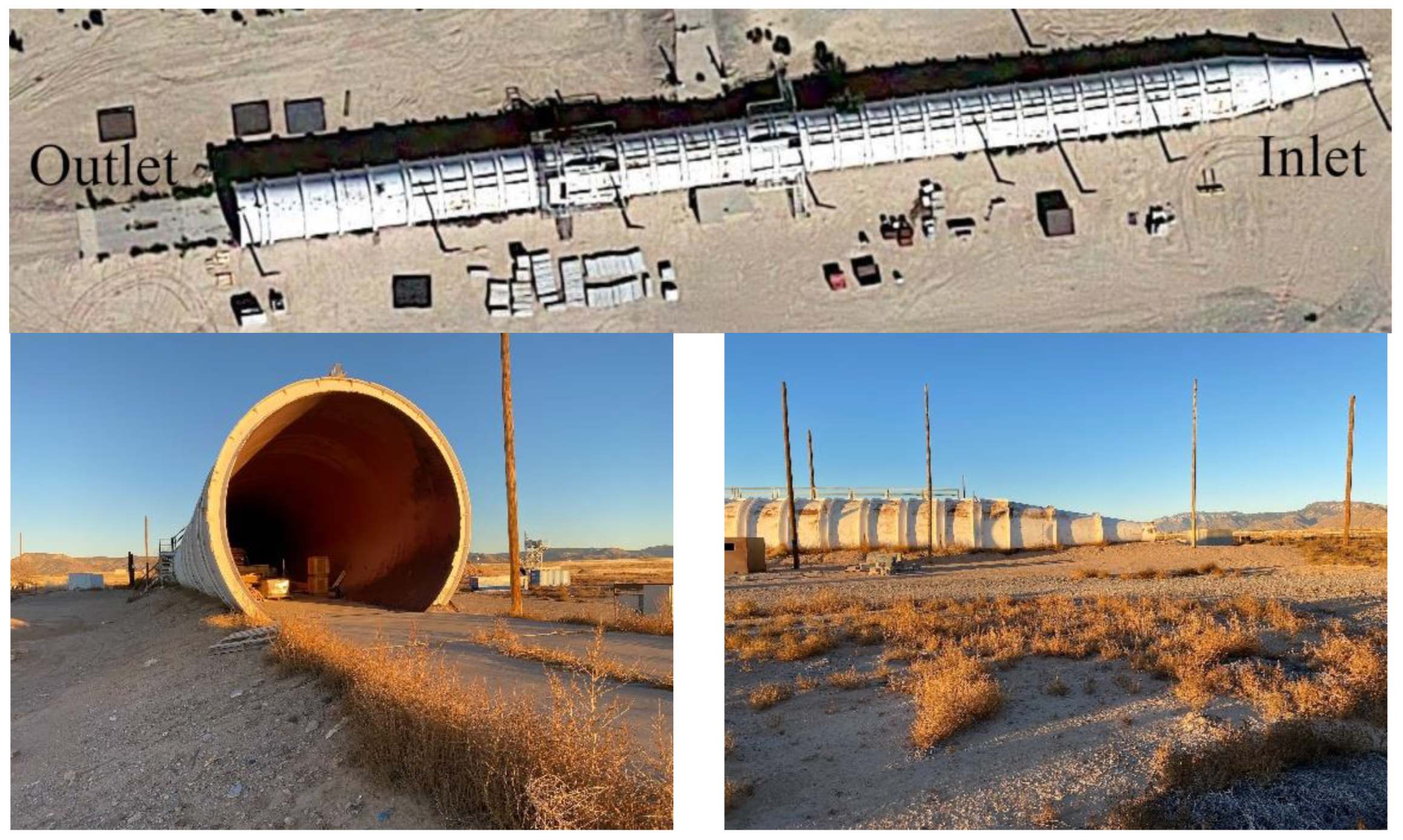
Sandia National Laboratories’ Shock Tube Facility at Thunder Range offered an excellent compromise between the safety of holding a liquid hydrogen experiment outside and having control over wind and other elements that would come with an indoor experiment. This facility was originally designed to perform tests with energetic and hazardous materials. While the hydrogen will not intentionally be ignited for this experiment, there is no safety concern for this facility if it were to accidentally ignite. This facility consists of a 91 m (300 ft) long, 25 mm (1″) thick reinforced steel tube that has a diameter of 5.5 m (18 feet) and a 5.23 m (17′2″) wide flat floor of reinforced concrete. The top view, the end where the inflow fan is placed, and the outflow exit are shown in Figure 1. A section approximately half the length of the tube has available openings to allow for piping in of the liquid hydrogen.
In order to simulate realistic outside wind conditions, a 2800 m3/min (100,000 ft3/min) fan was placed at the narrower end of the tube. This fan can be adjusted using a variable frequency drive to create several desired wind speeds for the tests. Filters were placed 11.6 m (38 feet) downstream of the fan to help the flow be more homogeneous, and help remove any dust or other particles. There will be tests conducted with air flow speeds of 0.45, 0.89, 1.34, 1.79, and 2.24 m/s (1, 2, 3, 4, and 5 mph) at the hydrogen test section. The flow in the tube will be carefully characterized using an anemometer before the hydrogen tests are performed. The wind speed will also be monitored at a single point upstream of the hydrogen pool during the tests. Temperatures on and throughout the concrete substrate will be measured, as well as those on the steel substrate. An array of thermocouples will be arranged in the downstream plume with sensors concentrated in areas where high concentrations of hydrogen are expected, as informed by this work. These thermocouples will be used to calculate concentrations, and those concentration measurements will be verified by a lower density of extractive concentration sensors.
2.2.2. CUBIT Meshing Software and Domain
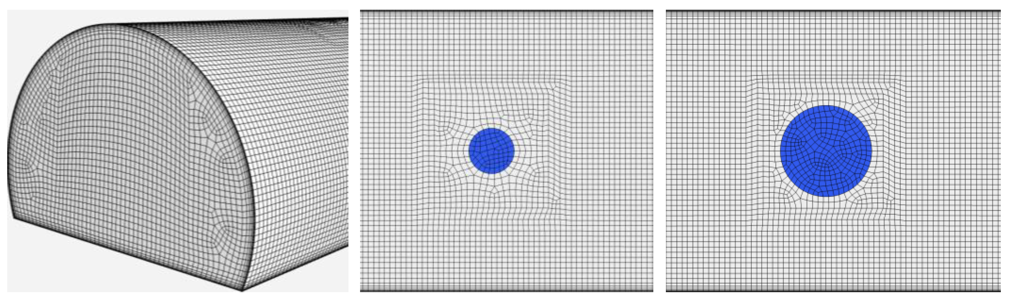
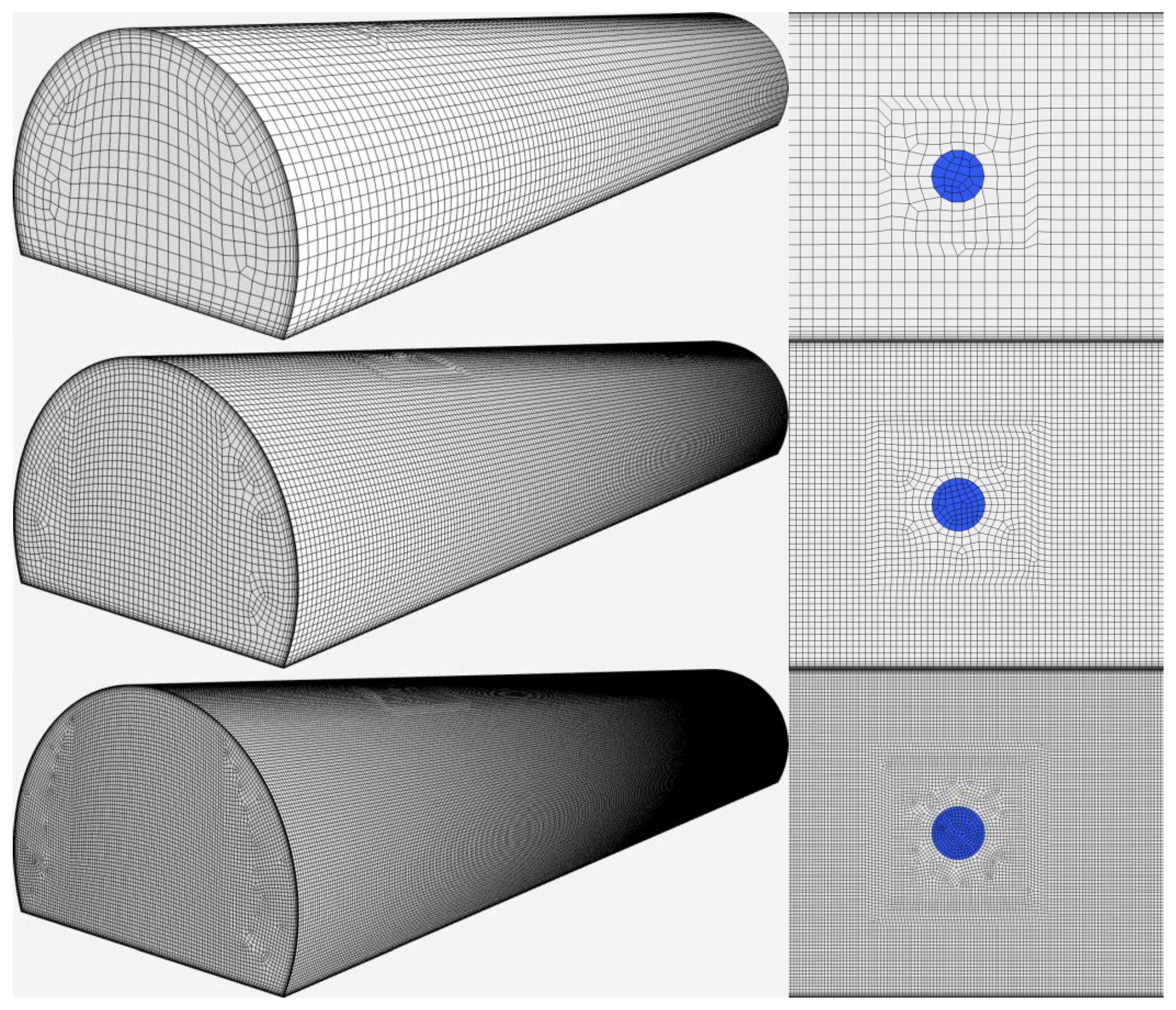
CUBIT is a full-featured software toolkit developed at Sandia National Laboratories for robust generation of two- and three-dimensional finite element meshes. Meshes with a combination of a structured boundary layer near walls and unstructured hexahedral elements were used for these simulations. Only the test section of the Shock Tube Facility was modeled, with 5.85 m (19 ft) before the center of the pool and 22.875 m (75 ft) after. The mesh, including a bottom-up view of both pools, is shown in Figure 2. The boundary layers had 8 nodes vertically from all walls, with spacings stretching from 5 mm to 86 mm. The unstructured hexahedral elements in the center of the domain matched the spacing of the boundary layer and were stretched to a maximum size of 0.1 m. The mesh was finer at and near the hydrogen inlet boundary surface which represented the liquid hydrogen pool (highlighted in blue in Figure 2. The pool with a diameter of 0.85 m had 67 elements, while the 1.7 m pool had 267 elements. The meshes had a total number of elements of 775,388 and 791,158 for the small and large pool, respectively.
2.2.3. Simulation Software
Fuego is a robust simulation software for buoyancy-driven turbulent flow mechanics [28,30]. This incompressible low-Mach CFD code is part of Sandia’s Sierra Suite [29]. Fuego uses an approximate projection algorithm with a control volume finite element method (CVFEM) [31]. The Reynolds-averaged Navier–Stokes (RANS) method was used to solve the time-dependent Navier–Stokes and energy equations. The two-equation standard k- closure model [32,33] is used to evaluate the turbulent eddy viscosity for RANS simulations.
We found that the choice of solvers did influence the shape of the hydrogen plume. The results presented here use the TPETRA equation solver using the PRESET scheme. The convergence tolerance was set to 1 × 10⁻⁸ for both continuity and scaler functions. The convection terms in the equations are discretized with a first-order upwind differencing scheme [34], using a hyperbolic tangent bending method with a shift of 1000 and width of 200 for the momentum equations, and a shift and width of 2 for continuity. Equations were solved using second-order-in-time.
Transport equations are solved for the mass fractions of each chemical species, except for the dominant species (nitrogen, in this case) which is computed by constraining the sum of the species mass fractions to equal one [35]. The density is based on the mixture fraction at a given node, and the temperature is solved through the Navier–Stokes equations, assuming ideal gas. Phase changes, of either the hydrogen, water, or air, are not taken into account.
There were five boundary conditions for these simulations. The floor and the curved walls to ceiling had a no-slip wall boundary condition applied. Because the modeling of the hydrogen vaporization was not carried out directly (see Section 2.3), heat transfer from the floor and sides of the tube were not considered. The wind flow was created by an inflow with a constant velocity for each of the five crosswind speeds. The outflow was an open boundary condition. The hydrogen pool was simulated as an inflow velocity, described in more detail in the next section. Buoyancy forces were calculated, and the ambient and buoyancy reference temperatures were set to T = 298 K.
2.3. Modeling of LH2 Pool and Vaporization
During the experiments, LH2 will be poured at a known rate onto the concrete where it will pool before boiling off. Modeling the pooling of liquid hydrogen and the phase change from liquid to vapor would add significant complexities to the modeling. Instead, a fixed pool size was assumed, and gaseous hydrogen at a temperature of T = 20 K is released upward into the domain with a velocity that will match the known flow rate of the experiment, 10 L/min. This method does not take into account the effect of the heat transfer from the ground on the vaporization rate, but instead approximates the rate using conservation of mass. Because the pool size will not be known until the experiment is completed, two bounding pool diameters were tested with the velocity adjusted accordingly. Using the saturation vapor density of hydrogen at 1.228 kg/m3, 10 L/min corresponds to a mass flow rate of 0.0117 kg/s, and the velocities of the cold hydrogen gas were set to 4.2 and 16.8 mm/s for pool diameters of 1.7, and 0.85 m, respectively.
2.4. Comparison of Simulations with Experiment
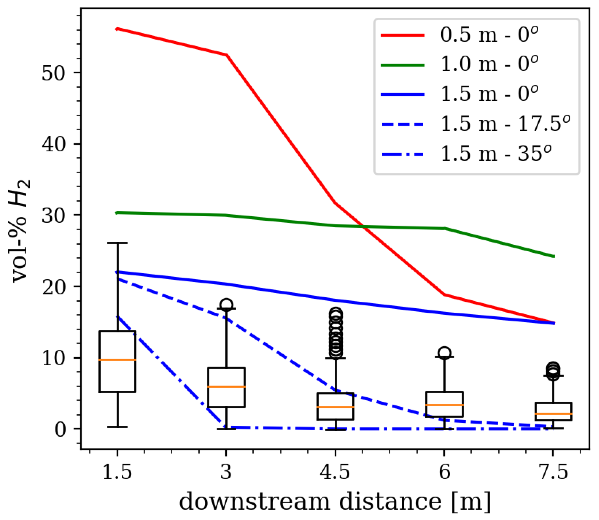
In order to validate our methodology and modeling parameters, simulations of the HSE-Test 6 [9,10] were performed. This was a vertically downward release 100 mm above the ground. The most applicable measurements to our work from this test are the hydrogen concentration measured at 5 distances downstream at a height of 0.25 m. The volume fractions in Figure 23 from [9] show instantaneous hydrogen concentrations at downstream distances of 1.5 m, 3.0 m, 4.5 m, 6.0 m, and 7.5 m. The data from this figure was extracted, and box-and-whisker plots of the concentration data are shown in Figure 3. They show that the highest volume fractions were measured at =1.5 m distance downstream, which has a maximum value around 26% and more typical volume fractions between 5 and 15%. At 3.0 m downstream, the maximum observed concentration was lower, at approximately 17%, with the majority of the data between about 4 and 8%. The measurements at 4.5, 6.0 and 7.5 m downstream have fairly similar median concentrations around 2–3%, with decreasing peak concentrations.
The simulations matched the HSE–Test 6 conditions: a wind speed of 2.675 m/s, an ambient temperature of 283.56 K, and a hydrogen mass flow rate of 0.07 kg/s. The pool size was estimated to be around 2.1 m × 1.3 m; we simulated a range of round pool diameters. The domain size is 40 m × 10 m × 12 m and had 54,723, 111,037, and 193,177 elements for pool diameters of 0.5, 1.0, and 1.5 m, respectively. The simulation parameters match those described in Section 2.2.3. The LH2 pool and vaporization modeling methodology is described in Section 2.3, and pool diameters of 0.5, 1.0, and 1.5 m were tested. Figure 3 shows the simulated concentrations at a height of 0.25 m going downstream from the pool. The solid lines are the concentrations along the centerline directly downstream of the pool. The simulated results along the centerline generally show a higher concentration than the median measured experimental values, which is in alignment with the findings of [17]. Although this method for introducing the hydrogen into the domain may cause an overprediction of the concentrations, it is expected that the location and shape of the plume are represented well enough to adequately plan for the sensor placements in the upcoming experiment. Another consideration of the higher concentrations comes with a closer examination of Figure 19 in [9], which shows the visible cloud passing mostly behind the poles (with the measurement sensors attached) at the time the picture was taken, rather than having the poles centered in the visible cloud. We assume from this that the measurement points were likely at an angle relative to the wind for some of the time during the measurements. To evaluate this effect, concentrations at a 17.5° and a 35° horizontal angle from the wind direction are also shown in Figure 3. The concentration, especially at further downstream distances, is much lower if the measurement is not along the centerline. In addition, unsteadiness in the wind also plays a large role in the variability in the concentration measurements. When accounting for the variation of the wind direction and speed, and uncertainty in the pool size during the experimental campaigns, our simulation concentrations align well with the data. The simulations for the 1.5 m diameter pool at 17.5° or greater from the centerline are well within the experimentally measured range at all distances from the release. This comparison highlights the challenges of using outdoor experiments to validate models.
3. Results
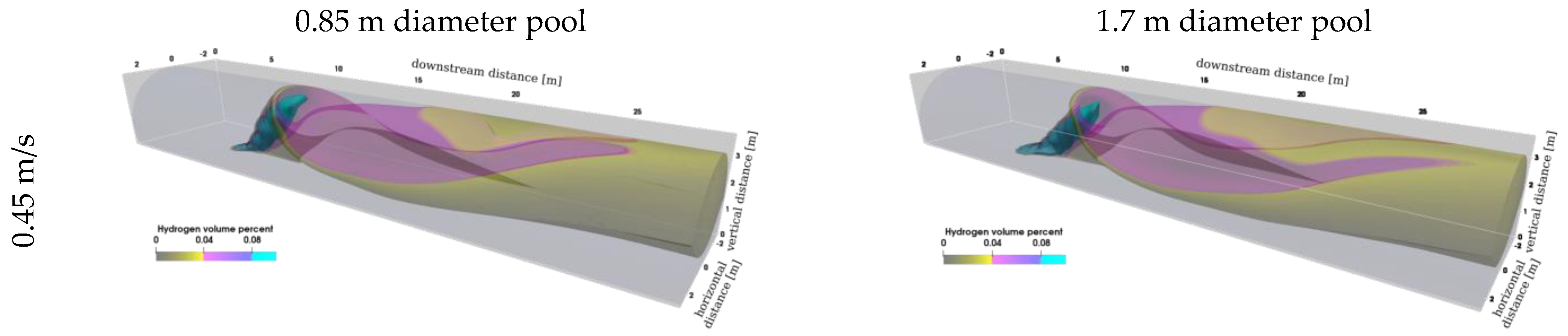
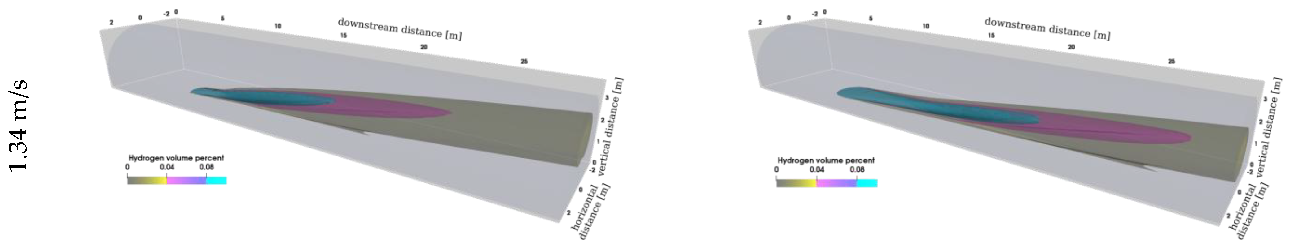
Hydrogen from the pool warms and mixes with air, becoming more dilute as the mixture travels downwind. The locations of the 4% and 8% mole fraction contours are shown in a three-dimensional view for several cases in Figure 4. For turbulent plumes, sustained light-up to a flame will occur at a mean mole fraction much higher than the 4% lower flammability limit; it will occur, typically, above 8% [36], so this contour is more representative of an area to avoid ignition sources than the mean 4% mole fraction contour. In all cases, near the pool, the density of the hydrogen is near that of air and the plume remains close to the floor. Downwind of the pool, there is some buoyancy to the mixture, and the 4% and 8% mole fraction isovolumes extend off the floor. As expected, this angle is steeper for the 0.45 m/s crosswind than the 1.34 m/s crosswind. The hydrogen is pushed towards the facility exit by the crosswind and exits through the outlet after interacting with the ceiling, in the 0.45 m/s case, or before interacting with the ceiling, in the 1.34 m/s case. Because the larger 1.7 m diameter pool has less upward momentum (because the volumetric flow rate of hydrogen is the same for both pool diameters), the wind pushes the flammable contours further downstream, and the contours remain closer to the ground than for the smaller pool diameter. The plume dispersion and the location of these 4 and 8% contours are the primary quantities of interest (QoIs) in this work, as these will inform the placement of the sensors during the experiments.
3.1. Mesh Refinement Study for the D = 0.85 m Pool
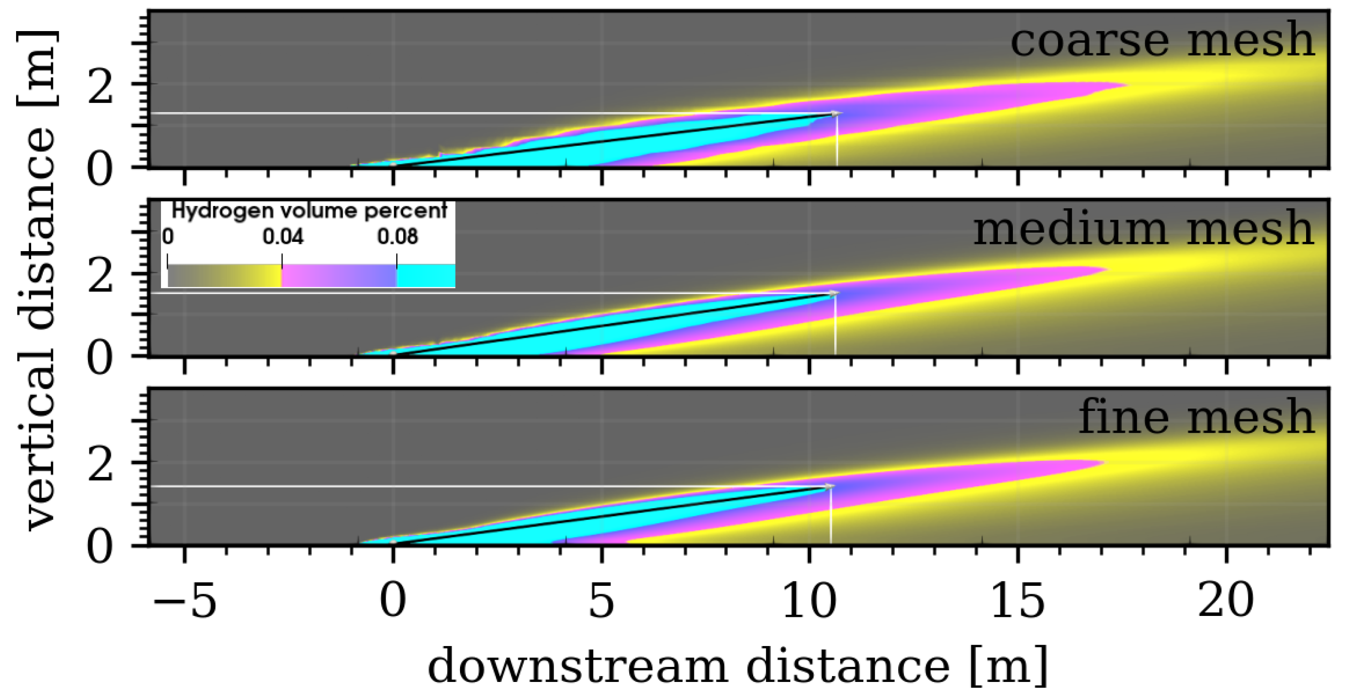
A mesh refinement study was completed to determine whether the mesh spacing used in the simulations accurately captures the flow physics and the QoIs. The QoIs include the length and height of the hydrogen plume, described by the location of the 8% mole fraction contour. This study uses the 1.34 m/s wind case and the LH2 pool diameter of 0.85 m. Three meshes, shown in Figure 5, were generated using Cubit. The coarse mesh has 127,234 elements and a mesh size of 0.2 m. The medium mesh (described previously) has 775,388 elements and a mesh size of 0.1 m. The finest mesh has 4,947,502 elements and a mesh size of 0.05 m. The number of elements that make up the surface of the pool are 26, 67, and 250 for the coarse, medium, and fine mesh, respectively.
The QoIs (location of the tip of the 8% mole fraction contour) from a course, medium, and fine mesh sizing are compared and shown in Table 1, and the centerline cross-sections showing an arrow from the center of the pool to the tip of the 8% mole fraction contour are shown in Figure 6. Close inspection of Figure 6 shows rough edges of the isocontours for the coarse mesh, which are artifacts from the coarseness of the mesh. Qualitatively, the plumes appear similar, and all three have similar values for the QoIs, shown in Table 1. Both the coarse and medium mesh results have a total plume length within 1.3% of the fine mesh. The difference in the length of the plume between the coarse and fine mesh is less than the spacing of the coarse mesh at the tip of the plume. The flammable mass, defined as the mass of hydrogen in the domain with mole fractions between 4 and 75% volume, increases slightly as the mesh becomes more refined, but in all cases is within 5% of the mass predicted by the fine mesh. Since the three mesh resolutions gave similar results for the QoIs, the medium mesh was chosen for the simulations, which was a good compromise between resolving the edges of the isocontours and the computational time required for convergence.
3.2. Plume Behavior
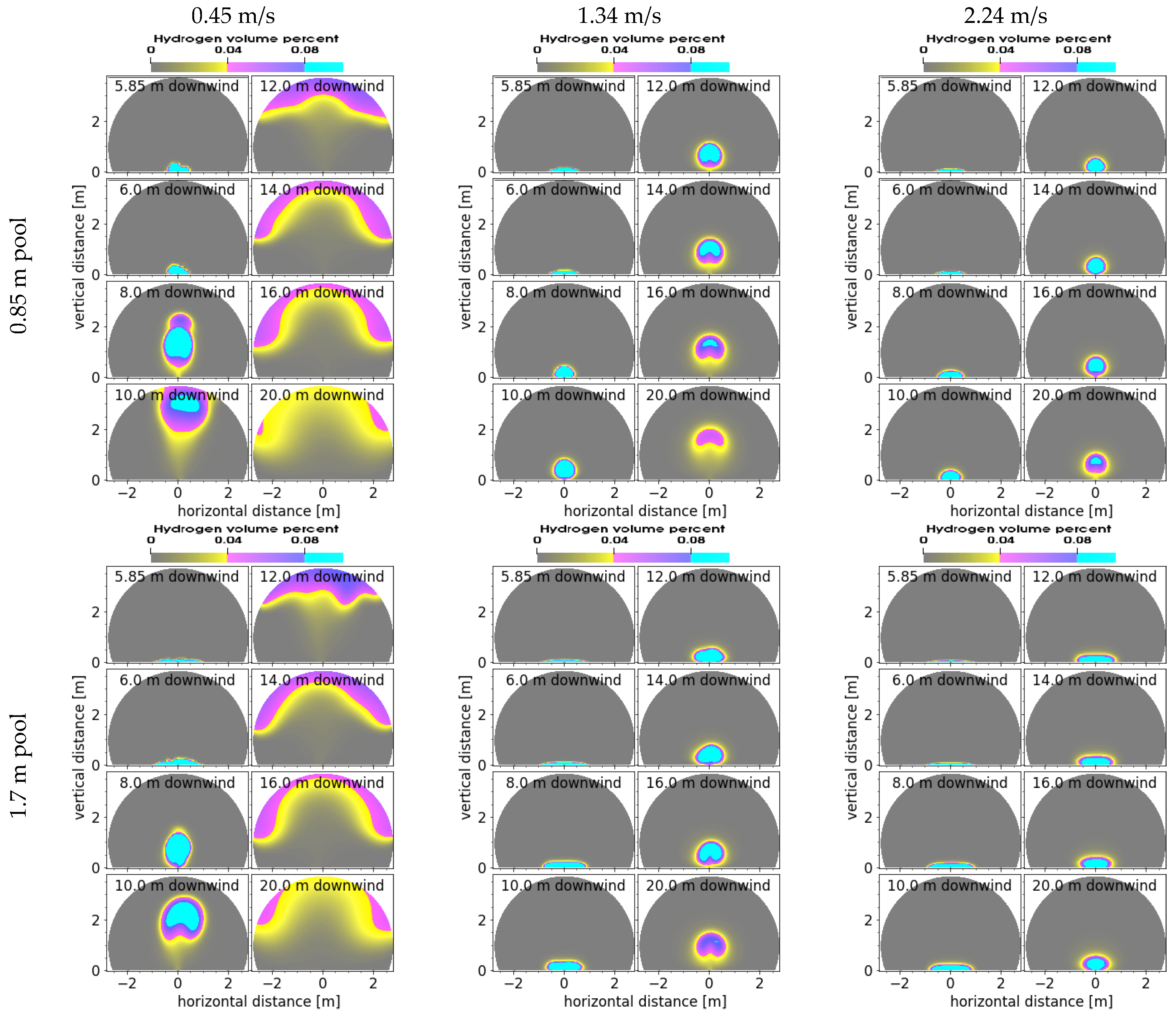
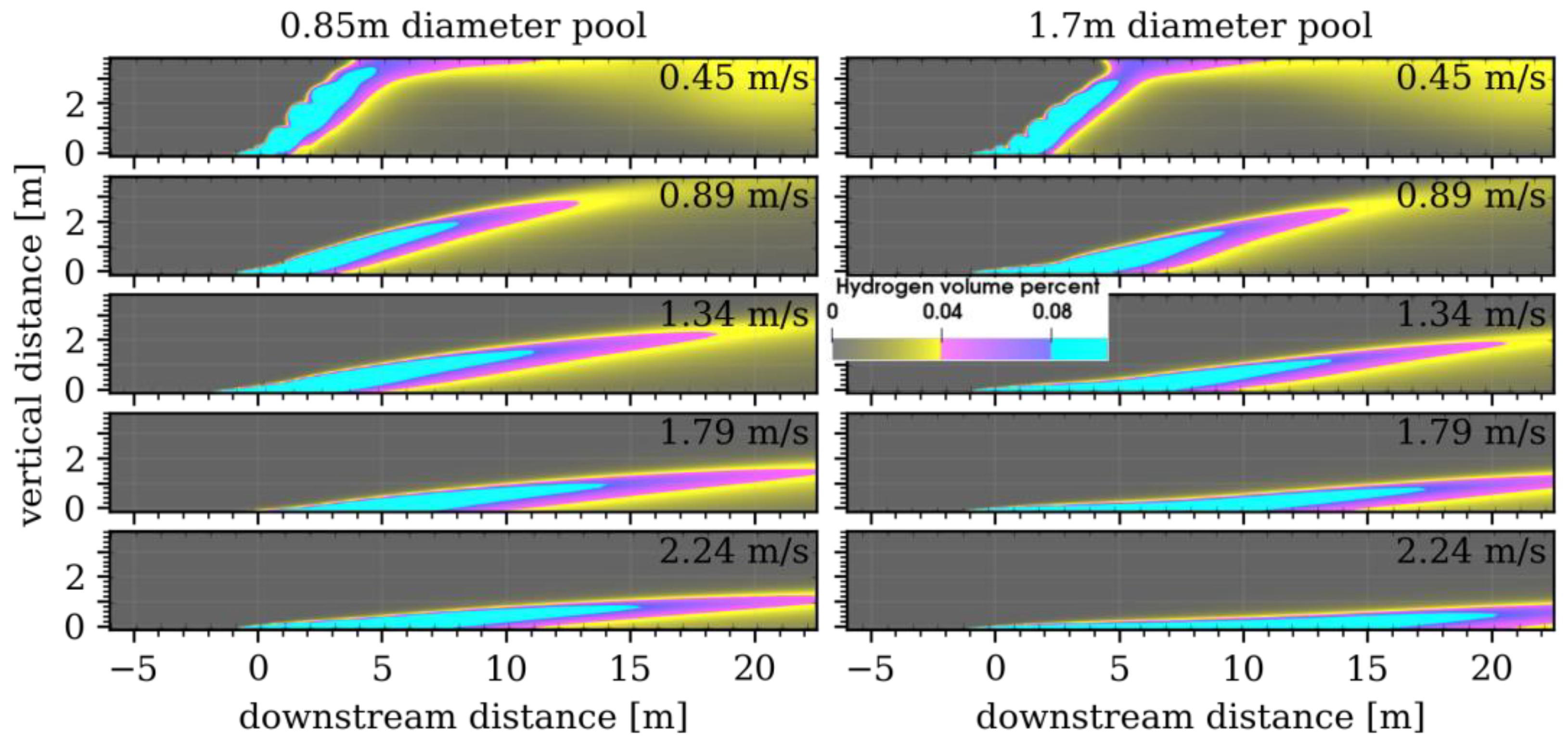
To help understand the shape and location of the plume, cross-sections for several conditions are shown in Figure 7. In all cases, the center of the pool in the first frame (5.85 m downwind) shows flammable mass extending only a few cm above the ground level. Only beyond the edge of the pool (8 m downwind) does the flammable mass (4% mole fraction contour) start to extend above ground level, and for the 2.24 m/s crosswind, not until 10 m downwind. In the later frames (>8 m downwind for the 0.45 m/s case, >10 m downwind for the 1.34 m/s cases, and > 14 m for the 0.85 m diameter pool in the 2.24 m/s case), there is no longer any flammable mass touching the floor, and the plume demonstrates a non-circular shape with some tucking in of the flammable mass on the bottom of the plume, as the vortices in the wake of the plume affect its shape. For the 0.45 m/s case, the plume can be seen reaching the ceiling 10–12 m downwind and then being pushed downwind along the curved ceiling of the Shock Tube Facility, and some hydrogen that is potentially flammable (>4%) is observed all the way to 20 m downwind. For the 3 and 2.24 m/s crosswinds, the hydrogen never reaches the ceiling. In all cases, the larger, 1.7 m diameter pool with the lower upward momentum of hydrogen, shows hydrogen remaining closer to the floor than the smaller pool for each downwind location. For the 2.24 m/s crosswind and the 1.7 m diameter pool, the flammable hydrogen mass remains in contact with the floor all the way to 20 m downwind, and almost to the facility exit.
3.3. Profiles along the Centerline
The centerline profiles for all 5 wind speeds are shown in Figure 8. As discussed previously, when comparing the left-hand frames for the 0.85 m diameter pool to the right-hand frames for the 1.7 m diameter pool, the smaller pool diameter, with a higher upward hydrogen momentum, tends to have a plume that extends further vertically rather than horizontally. As with Figure 7, but more explicitly shown here, the 4% mole fraction contour only touches the ceiling for the 0.45 m/s crosswind, and the 4% contour is swept out of the Shock Tube Facility exit for 4 mph or greater crosswind for both plumes. While the pool diameter has a small effect on the plume shapes, it is much less of a factor than the crosswind. This implies that during the experiments, the plume measurements can be set up for a certain crosswind and will not be overly affected by unsteady pool dimensions, which will occur as the substrate temperature changes.
3.4. Summary of Plume Shape
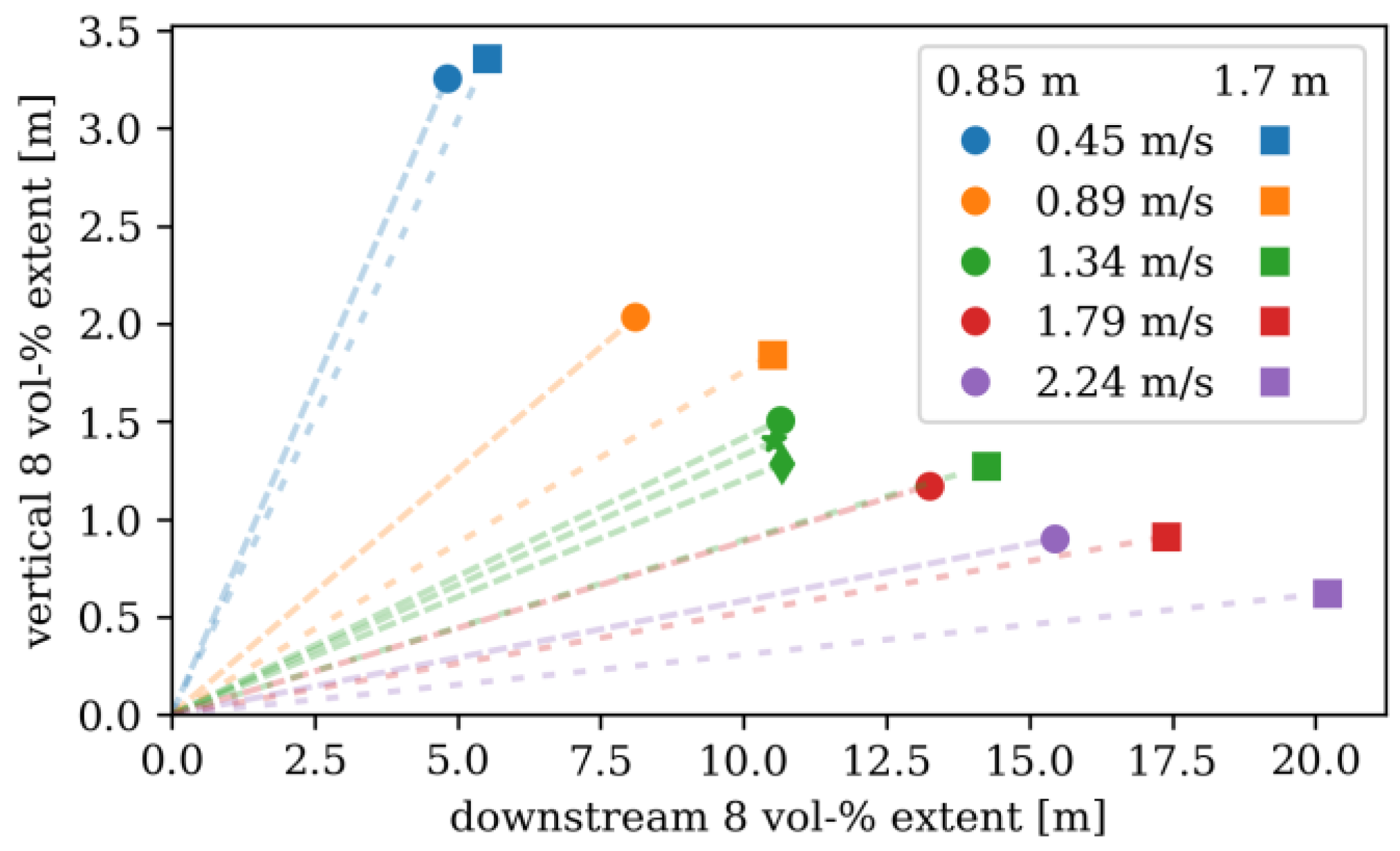
As might be expected and was discussed previously, with increasing crosswind speed, the plume tends to stretch further downwind and remain closer to ground level. A comparison of the maximum extent of the average 8% mole fraction, vertically and horizontally, is graphically shown in Figure 9. For the 1.7 m diameter pool, the lower initial upward momentum reduces the height of the plume and causes extension further downstream for a given wind speed, as can be seen by comparing the square symbols to the circular symbols for a given color. It should be noted that for at least the slowest wind speed of 0.45 m/s, there is obvious interaction with the ceiling of the tube, and the height of the plume is expected to be taller for releases that are outside. Figure 9 also includes the mesh sensitivity study, performed for the 1.34 m/s, 0.85 m pool simulation. The extent of the plume changes slightly for the coarser and finer mesh, but was deemed to be sufficiently stable for the level of detail needed for these results.
3.5. Flammable Mass Evolution
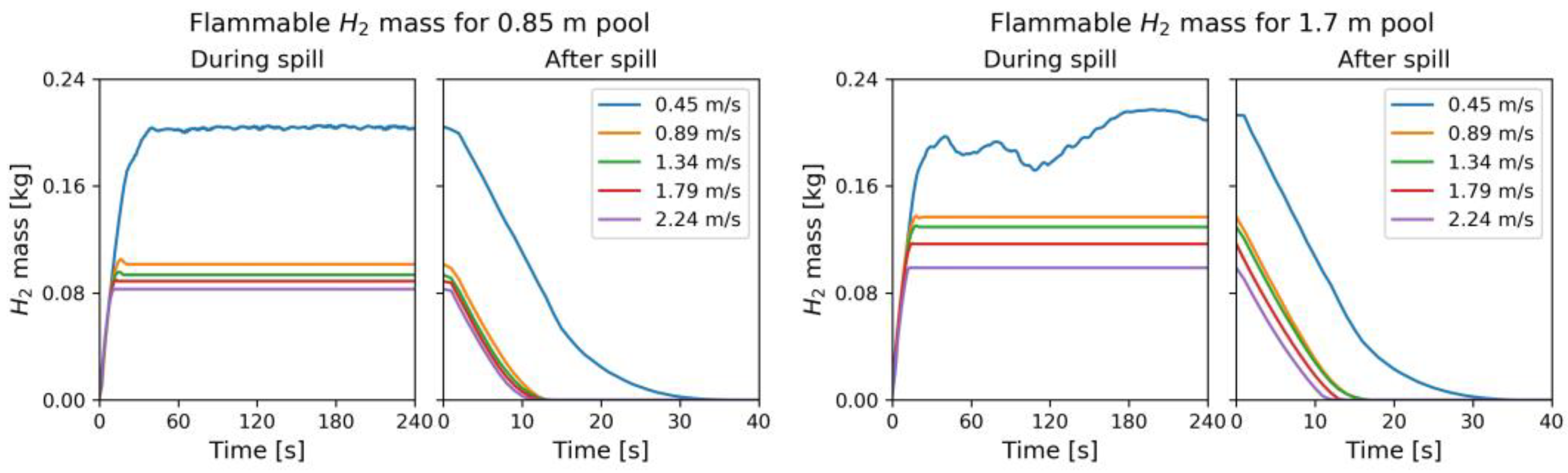
The flammable mass was calculated by integrating the product of the hydrogen mass fraction and the density of the gas over the volume where the mole fraction was between 4 and 75%. The temporal evolution of this flammable mass is shown in Figure 10. Increasing the wind speed increases the dilution of the hydrogen, and the steady-state flammable mass decreases with wind speed. A steady flammable mass is reached within the first minute of starting the hydrogen flow, with less time required to reach steady-state for higher wind speeds. The 1.7 m pool diameter shows significant unsteadiness for the 0.45 m/s crosswind, likely due to interactions with the ceiling and walls. For a given crosswind speed, the larger, 1.7 m pool release generates a higher steady-state flammable mass than the smaller pool. In addition to the fact that the two pools will result in different plume dimensions, which affects mixing, the plume from the larger pool, with less upward momentum, remains in contact with the floor for a longer distance, which decreases dilution from the bottom of the plume.
4. Discussion and Conclusions
The main purpose of the simulation results presented in this paper is to help inform experimental design and sensor placement for an upcoming experimental campaign which will be a series of liquid hydrogen releases inside of Sandia National Laboratories’ Shock Tube Facility. The experiments will utilize this facility to safely work with liquid hydrogen while controlling wind conditions, in an attempt to generate high quality data suitable for model validation. While LES simulations would better capture the turbulence in the plumes, it was determined that RANS would be suficient for caputuring the quantities of interest needed to contribute to the planning of the experiment.
A RANS model of the experimental facility demonstrated that the hydrogen plume becomes longer and remains closer to the ground with increasing wind speed. For a spill rate of 10 L/min, the plume height (as defined by the 8% mole fraction contour) ranged from reaching over 3 m high to staying under 1 m high. The length increased from 5 m during 0.45 m/s wind speed to 20 m with 2.24 m/s speeds. While heat exchange between the ground and hydrogen pool, and the condensation or solidification of the moisture, oxygen and nitrogen in the air were not modeled, the RANS model captured the trends observed by simulations of previous experiments: increased wind speed expands the downwind distance of the flammable plume and decreases the plume height. One thing to note is that for the lower wind speeds, it is likely that the hydrogen plume will reach the ceiling of the Shock Tube. This will of course limit the height of the plume, and affect the plume in other ways. For this reason, at lower wind speeds we expect the plume in the experiment to be the most different that from what would be experienced for an outdoor release with no confining walls. Because of this, higher wind speeds are in the experimental plan to make it less likely that the plume will interact with the ceiling of the tube.
Without a priori knowledge of the width of the pool, two pool diameters were simulated. Even though the mass flow rate was kept the same between these two cases, the width of the pool did have an effect on the shape of the plume and the amount of flammable hydrogen found in the domain. Except for the 0.45 m/s crosswind case, which experiences interactions with ceiling and sides of the tube, the plume from the wider pool is both longer and remains closer to the ground. The change in the shape of the plume also results in a slightly higher amount of flammable mass reached at a steady state for the cases with the wider pool. Although the pool diameter does affect the plume shape, the wind speed has a greater effect.
The conclusions relating to conducting the experiment are that the sensors that will be used to measure the hydrogen concentration and the temperature will need to be reconfigured for each wind speed tested. More sensors will be placed closer to the ground and farther downstream from the relaease point for higher wind speeds. The sensors might also need to be adjusted depending on the ultimate size of the pool of hydrogen. Knowing this, an adjustable rig will be used so that the height, width, and downstream measurements can be changed to best match the wind speed and other conditions.
While we are anticipating many more insights into liquid hydrogen leaks from the experiments, from these preliminary simulations, it can be concluded that the height and length of the flammable plume is highly dependent on the wind, and any confinement of the pool on the ground will also result in a taller plume. While the intent of the experiment is to mimic conditions outside, the results from both this study as well as the experiment are very applicable to hydrogen spills inside a tunnel. These results indicate that even with minor ventilation, the hydrongen plume would be swept significantly far away from the release point.
Author Contributions
Conceptualization, K.M.G., M.B. and E.S.H.; Formal analysis, K.M.G.; Funding acquisition, E.S.H.; Investigation, K.M.G. and M.B.; Methodology, K.M.G., M.B. and E.S.H.; Project administration, E.S.H.; Validation, K.M.G.; Visualization, K.M.G., M.B. and E.S.H.; Writing—original draft, K.M.G., M.B. and E.S.H.; Writing—review and editing, K.M.G., M.B. and E.S.H. All authors have read and agreed to the published version of the manuscript.
Funding
This work was accomplished through funding from the U.S. Department of Energy’s Hydrogen and Fuel Cell Technologies Office.
Data Availability Statement
This article has been authored by an employee of National Technology & Engineering Solutions of Sandia, LLC under Contract No. DE-NA0003525 with the U.S. Department of Energy (DOE). The employee owns all right, title and interest in and to the article and is solely responsible for its contents. The United States Government retains and the publisher, by accepting the article for publication, acknowledges that the United States Government retains a non-exclusive, paid-up, irrevocable, world-wide license to publish or reproduce the published form of this article or allow others to do so, for United States Government purposes. The DOE will provide public access to these results of federally sponsored research in accordance with the DOE Public Access Plan. This paper describes objective technical results and analysis. Any subjective views or opinions that might be expressed in the paper do not necessarily represent the views of the U.S. Department of Energy or the United States Government.
Acknowledgments
The authors would like to thank the experimental team for discussions on the planned setup, including Walt Gill, Carl Fitzgerald, Pasqual Vallejos, Kyle Winter, Alvaro Cruz-Cabrera, and Anay Luketa.
Conflicts of Interest
The authors declare no conflict of interest. The funders had no role in the design of the study; in the collection, analyses, or interpretation of data; in the writing of the manuscript, or in the decision to publish the results.
References
- Aurther, D. Little, Inc. Final Report on an Investigation of Hazards Associated with the Storage and Handling of Liquid Hydrogen; Report no. C-61092; U.S. Air Force Ballistic Missle Division: Los Angeles, CA, USA, 1960.
- Zabetakis, M.G.; Burgess, D.S. Research on Hazards Associated with Production and Handling of Liquid Hydrogen. [Fire Hazards and Formation of Shock-Sensitive Condensed Mixtures]; U.S. Department of the Interior, Bureau of Mines: Washington, DC, USA, 1961.
- Zabetakis, M.G.; Furno, A.L.; Martindill, G.H. Explosion Hazards of Liquid Hydrogen. In Advances in Cryogenic Engineering; Springer: Boston, MA, USA, 1961; Volume 6, pp. 185–194. [Google Scholar] [CrossRef]
- Witcofski, R.D.; Chirivella, J.E. Experimental and Analytical Analyses of the Mechanisms Governing the Dispersion of Flammable Clouds Formed by Liquid Hydrogen Spills. Int. J. Hydrogen Energy 1984, 9, 425–435. [Google Scholar] [CrossRef]
- Verfondern, K.; Dienhart, B. Pool spreading and vaporization of liquid hydrogen. Int. J. Hydrogen Energy 2007, 32, 2106–2117. [Google Scholar] [CrossRef]
- Verfondern, K.; Dienhart, B. Experimental and theoretical investigation of liquid hydrogen pool spreading and vaporization. Int. J. Hydrogen Energy 1997, 22, 649–660. [Google Scholar] [CrossRef]
- Schmidtchen, U.; Marinescu-Pasoi, L.; Verfondern, K.; Nickel, V.; Strum, B.; Dienhart, B. Simulation of accidental spills of cryogenic hydrogen in a residential area. Cryogenics 1994, 34, 401–404. [Google Scholar] [CrossRef]
- Dienhart, B. Ausbreitung und Verdampfung von flussigem Wasserstoff auf Wasser und festem Untergrund; Forschungszentrum Jülich GmbH: Jülich, Germany, 1995. [Google Scholar]
- Royle, M.; Willoughby, D. Releases of Unignited Liquid Hydrogen; RR986; Health and Safety Executive: Buxton, UK, 2014.
- Hooker, P.; Willoughby, D.; Royle, M. Experimental releases of liquid hydrogen. In Proceedings of the International Conference on Hydrogen Safety, San Francisco, CA, USA, 12–14 September 2011. [Google Scholar]
- Lyons, K.; Coldrick, S.; Atkinson, G. Summary of Experiment Series E3.5 (Rainout) Results; PRESLHY deliverable D3.6. 2020. Available online: https://hysafe.info/wp-content/uploads/sites/3/2020/08/PRESLHY_D3.6_Summary_of_Rainout_Experiments_V1.20.pdf (accessed on 1 February 2023).
- Buttner, W.; Hall, J.; Coldrick, S.; Hooker, P.; Wischmeyer, T. Hydrogen wide area monitoring of LH2 releases. Int. J. Hydrogen Energy 2021, 46, 12497–12510. [Google Scholar] [CrossRef]
- Medina, C.H.; Halford, A.; Stene, J.; Allason, D. Data Report: Outdoor Leakage Studies; Report no. 853182, Rev. 2.; DNV GL Oil and Gas, Spadeadam Testing and Research: Brampton, UK, 2020. [Google Scholar]
- Shao, X.; Pu, L.; Li, Q.; Li, Y. Numerical investigation of flammable cloud on liquid hydrogen spill under various weather conditions. Int. J. Hydrogen Energy 2018, 43, 5249–5260. [Google Scholar] [CrossRef]
- Jin, T.; Wu, M.; Liu, Y.; Lei, G.; Chen, H.; Lan, Y. CFD modeling and analysis of the influence factors of liquid hydrogen spills in open environment. Int. J. Hydrogen Energy 2017, 42, 732–739. [Google Scholar] [CrossRef]
- Molkov, V.V.; Makarov, D.; Prost, E. On Numerical Simulation of Liquefied and Gaseous Hydrogen Releases at Large Scales. In Proceedings of the International Conference on Hydrogen Safety, Pisa, Italy, 8–10 September 2005. [Google Scholar]
- Venetsanos, A.G.; Bartzis, J.G. CFD modeling of large-scale LH2 spills in open environment. Int. J. Hydrogen Energy 2007, 32, 2171–2177. [Google Scholar] [CrossRef]
- Statharas, J.; Venetsanos, A.; Bartzis, J.; Würtz, J.; Schmidtchen, U. Analysis of data from spilling experiments performed with liquid hydrogen. J. Hazard. Mater. 2000, 77, 57–75. [Google Scholar] [CrossRef] [PubMed]
- Ichard, M.; Hansen, O.R.; Middha, P.; Willoughby, D. CFD computations of liquid hydrogen releases. Int. J. Hydrogen Energy 2012, 37, 17380–17389. [Google Scholar] [CrossRef]
- Pu, L.; Tang, X.; Shao, X.; Lei, G.; Li, Y. Numerical investigation on the difference of dispersion behavior between cryogenic liquid hydrogen and methane. Int. J. Hydrogen Energy 2019, 44, 22368–22379. [Google Scholar] [CrossRef]
- Giannissi, S.G.; Venetsanos, A.G.; Markatos, N.; Bartzis, J.G. CFD modeling of hydrogen dispersion under cryogenic release conditions. Int. J. Hydrogen Energy 2014, 39, 15851–15863. [Google Scholar] [CrossRef]
- Liu, Y.; Wei, J.; Lei, G.; Chen, H.; Lan, Y.; Gao, X.; Wang, T.; Jin, T. Spread of hydrogen vapor cloud during continuous liquid hydrogen spills. Cryogenics 2019, 103, 102975. [Google Scholar] [CrossRef]
- Hansen, O.R.; Hansen, E.S. CFD-modelling of large scale LH2 release experiments. Chem. Eng. Trans. 2022, 90, 619–624. [Google Scholar]
- Pu, L.; Shao, X.; Zhang, S.; Lei, G.; Li, Y. Plume dispersion behaviour and hazard identification for large quantities of liquid hydrogen leakage. Asia-Pac. J. Chem. Eng. 2019, 14, e2299. [Google Scholar] [CrossRef]
- Giannissi, S.G.; Venetsanos, A.G. Study of key parameters in modeling liquid hydrogen release and dispersion in open environment. Int. J. Hydrogen Energy 2018, 43, 455–467. [Google Scholar] [CrossRef]
- Giannissi, S.G.; Venetsanos, A.G. A comparative CFD assessment study of cryogenic hydrogen and LNG dispersion. Int. J. Hydrogen Energy 2019, 44, 9018–9030. [Google Scholar] [CrossRef]
- Sandia National Laboratories. Cubit. Available online: https://cubit.sandia.gov/ (accessed on 1 February 2023).
- Moen, C.; Evans, G.H.; Domino, P.; Burns, S.P. A multi-mechanics approach to computational heat transfer. In Proceedings of the ASME 2002 International Mechanical Engineering Congress and Exposition. Heat Transfer, New Orleans, LA, USA, 17–22 November 2002; ASME: New York, NY, USA; Volume 6, pp. 25–32. [CrossRef]
- Shaw, R.P.; Agelastos, A.M. Guide to Using Sierra; SAND-2019-2865673446; Sandia National Laboratories: Albuquerque, NM, USA, 2019. [CrossRef]
- Nalu Development Team. Sierra Low Mach Module: Nalu - Theory Manual. Available online: https://nalu.readthedocs.io/en/latest/source/theory/index.html (accessed on 1 February 2023).
- Schefer, R.; Houf, W.G.; Bourne, B.; Colton, J. Spatial and radiative properties of an open-flame hydrogen plume. Int. J. Hydrogen Energy 2006, 31, 1332–1340. [Google Scholar] [CrossRef]
- Wilcox, D.C. Turbulence Modeling for CFD, 2nd ed.; DCW Industries: La Cañada, CA, USA, 1998. [Google Scholar]
- Launder, B.E.; Spalding, D.B. The numerical computation of turbulent flows. Comput. Methods Appl. Mech. Eng. 1974, 3, 269–289. [Google Scholar] [CrossRef]
- Barth, T.; Jespersen, D. The design and application of upwind schemes on unstructured meshes. In Proceedings of the 27th Aerospace Sciences Meeting, Reno, NV, USA, 9–12 January 1989. [Google Scholar] [CrossRef]
- Goodwin, D.G.; Moffat, H.K.; Schoegl, I.; Speth, R.L.; Weber, B.W. Cantera: An object-oriented software toolkit for chemical kinetics, thermodynamics, and transport processes. Version 2.6.0. 2022. Available online: https://www.cantera.org (accessed on 1 February 2023).
- Schefer, R.W.; Evans, G.H.; Zhang, J.; Ruggles, A.J.; Greif, R. Ignitability limits for combustion of unintended hydrogen releases: Experimental and theoretical results. Int. J. Hydrogen Energy 2011, 36, 2426–2435. [Google Scholar] [CrossRef]
Figure 1.
Satellite view (top) and photos (bottom) of the outlet (left) and inlet (right) of the Shock Tube.
Figure 1.
Satellite view (top) and photos (bottom) of the outlet (left) and inlet (right) of the Shock Tube.

Figure 2.
Mesh used for the simulations, with a 3D view of the wind inlet on the left, and a zoomed in view from the bottom of the 0.85 m (center) and 1.7 m (right) diameter pool.
Figure 2.
Mesh used for the simulations, with a 3D view of the wind inlet on the left, and a zoomed in view from the bottom of the 0.85 m (center) and 1.7 m (right) diameter pool.

Figure 3.
Box-and-whisker plots show the measured concentrations from HSE–Test 6 (data were extracted from Figure 23 in [9]). The hydrogen concentrations from Fuego simulations are shown going downstream with the measurement points at a height of 0.25 m along the centerline (solid line), at a 17.5° (dashed line) and at a 35° (dot-dashed line) horizontal angle from the wind direction. Results for the three pool diameters are shown as described in the legend: 0.5 m (red), 1.0 m (green), and 1.5 m (blue).

Figure 4.
Isovolume contours of 4% and 8% mole fractions for the 0.85 m (left) and 1.7 m diameter pool (right) with 0.45 m/s (top) and 1.34 m/s (bottom) crosswinds.
Figure 4.
Isovolume contours of 4% and 8% mole fractions for the 0.85 m (left) and 1.7 m diameter pool (right) with 0.45 m/s (top) and 1.34 m/s (bottom) crosswinds.


Figure 5.
The coarse, medium, and fine meshes in the top, middle, and bottom panels, respectively, with a bottom-up view of the mesh around the pool shown on the right.
Figure 5.
The coarse, medium, and fine meshes in the top, middle, and bottom panels, respectively, with a bottom-up view of the mesh around the pool shown on the right.

Figure 6.
Profiles along the centerline of the Thunder Pipe for a 1.34 m/s crosswind and the 0.85 m pool with different mesh resolutions.
Figure 6.
Profiles along the centerline of the Thunder Pipe for a 1.34 m/s crosswind and the 0.85 m pool with different mesh resolutions.

Figure 7.
Cross-sections of the 4% and 8% mole fractions at selected downwind distances for the 0.85 m (top) and 1.7 m (bottom) diameter pool at three crosswind speeds, as shown in the top labels, after the plume is at steady-state.
Figure 7.
Cross-sections of the 4% and 8% mole fractions at selected downwind distances for the 0.85 m (top) and 1.7 m (bottom) diameter pool at three crosswind speeds, as shown in the top labels, after the plume is at steady-state.

Figure 8.
Profiles along the centerline of the shock tube for both diameter pools and all crosswind flow rates after the plume is at steady-state.
Figure 8.
Profiles along the centerline of the shock tube for both diameter pools and all crosswind flow rates after the plume is at steady-state.

Figure 9.
Maximum extent of the 8% mole fraction, vertically and downstream, for the two different pool sizes. The star and diamond symbols are also simulations for the 0.85 m diameter pool, using a coarse and fine mesh, respectively.
Figure 9.
Maximum extent of the 8% mole fraction, vertically and downstream, for the two different pool sizes. The star and diamond symbols are also simulations for the 0.85 m diameter pool, using a coarse and fine mesh, respectively.

Figure 10.
Evolution of flammable mass within for the two different pool diameters as a function of wind speed. For the second frame in each case, time 0 represents when the hydrogen inflow was set to 0.
Figure 10.
Evolution of flammable mass within for the two different pool diameters as a function of wind speed. For the second frame in each case, time 0 represents when the hydrogen inflow was set to 0.


Table 1.
The quantities of interest for the mesh refinement study are the plume downstream distance, height, angle from the floor, and the steady-state flammable mass. These were all simulated with a wind speed of 1.34 m/s and a pool diameter of 0.85 m.
Table 1.
The quantities of interest for the mesh refinement study are the plume downstream distance, height, angle from the floor, and the steady-state flammable mass. These were all simulated with a wind speed of 1.34 m/s and a pool diameter of 0.85 m.
| Mesh | Total Length (m) | Height (m) | Angle (deg) | Flammable Mass (kg) |
|---|---|---|---|---|
| coarse | 10.67 | 1.28 | 6.86 | 0.091 |
| medium | 10.63 | 1.51 | 8.06 | 0.094 |
| fine | 10.53 | 1.40 | 7.56 | 0.095 |
Disclaimer/Publisher’s Note: The statements, opinions and data contained in all publications are solely those of the individual author(s) and contributor(s) and not of MDPI and/or the editor(s). MDPI and/or the editor(s) disclaim responsibility for any injury to people or property resulting from any ideas, methods, instructions or products referred to in the content. |
© 2023 by the authors. Licensee MDPI, Basel, Switzerland. This article is an open access article distributed under the terms and conditions of the Creative Commons Attribution (CC BY) license (https://creativecommons.org/licenses/by/4.0/).
Share and Cite
MDPI and ACS Style
Mangala Gitushi, K.; Blaylock, M.; Hecht, E.S. Simulations for Planning of Liquid Hydrogen Spill Test. Energies 2023, 16, 1580. https://0-doi-org.brum.beds.ac.uk/10.3390/en16041580
AMA Style
Mangala Gitushi K, Blaylock M, Hecht ES. Simulations for Planning of Liquid Hydrogen Spill Test. Energies. 2023; 16(4):1580. https://0-doi-org.brum.beds.ac.uk/10.3390/en16041580
Chicago/Turabian StyleMangala Gitushi, Kevin, Myra Blaylock, and Ethan S. Hecht. 2023. "Simulations for Planning of Liquid Hydrogen Spill Test" Energies 16, no. 4: 1580. https://0-doi-org.brum.beds.ac.uk/10.3390/en16041580
Note that from the first issue of 2016, this journal uses article numbers instead of page numbers. See further details here.