
Numerical Investigation of a Novel Controlled-Temperature Double-Skin Façade (DSF) Building Element


School of Engineering, Frederick University, Nicosia 1036, Cyprus
*
Author to whom correspondence should be addressed.
Energies 2023, 16(4), 1836; https://0-doi-org.brum.beds.ac.uk/10.3390/en16041836
Submission received: 2 January 2023
/
Revised: 26 January 2023
/
Accepted: 1 February 2023
/
Published: 12 February 2023
(This article belongs to the Special Issue Energy and Environmental Management of Buildings and Systems)
Abstract
:This paper investigates a novel controlled-temperature double-skin façade (DSF) building element. A three-dimensional time-dependent numerical model was developed for six different geometries for the investigation of thermal performance under different orientations (azimuth 0°, 90°, 180° and 270°). The boundary conditions of the numerical model were determined with the PVGIS tool and adjusted with the sol-air temperature equation. The results of the numerical simulation were validated with the use of measurements from an experimental test cell. The numerical results indicated an improved thermal performance when temperature-controlled air and flow were supplied through the building envelope with annual total energy savings in kWh/m2 of 1.99, 1.38, 2.13 and 2.06 for azimuth 0°, 90°, 180° and 270°, respectively. In regard to the total energy savings in %, the maximum benefit was considered to be in the winter season, with values of 65, 29, 80 and 28 for azimuth 0°, 90°, 180° and 270°, respectively. The experimental measurements revealed the test cell’s ability to maintain a relatively constant internal surface temperature and to not be significantly affected by the orientation and diverse ambient conditions.
1. Introduction
Double-skin façade (DSF) is an established solution with the potential to improve the thermal insulation performance of building masonry [1]. The energy performance of double-skin façades (DSF) and their impact on the building envelope is attainable with the use of numerical simulation modelling, experimental setup measuring or current building analysis. In recent studies of DSF investigation, several numerical models have been developed for the energy analysis of DSFs with the use of computational tools, such as ANSYS Fluent, ANSYS CFX, Energy Plus, TRNSYS, IDA ICE, IES-VE, MATLAB, Design Builder and IESVE. In particular studies, the impact of different geometric parameters on the DSF overall performance was investigated, with the following parameters:
The investigations of existing buildings were performed in some studies with the use of measurement equipment, such as data loggers, thermocouple sensors, or weather stations, and data were collected, and analyzed used for numerical model validation or building energy performance assessment [7,8,13]. Natural ventilation of (DSF) was considered in the study of [11], in which [2,4] mechanical ventilation was used. Regarding the environmental conditions, the developed numerical models utilized dynamic temperature and solar radiation profiles retrieved from online databases or measured data from the weather station and employed as boundary conditions [2,3,4,7,10,11,13,14,15,16,17]. In some studies, static solar radiation and temperature profiles were considered [9,12,18], whereas in other studies, wind speed was also counted as a boundary condition [2,7,13,15,16]. Regarding the results of the numerical model simulations or the acquired data from test cell configurations and existing buildings required for the energy performance assessment, the following data were retrieved:
- Temperature across the DSF, glazing, test cell structure (inner/outer), air indoors/outdoors, building wall (surface); ambient temperature.
- Sensible cooling/heating load.
- Solar radiation.
- Wind speed and air velocity inside the DSF.
- Heat flux and heat transfer through masonry.
The following studies compared the numerical results with the experimental results to validate the numerical model using the following methods:
- Mean bias error [13].
Table 1 presents the reviewed studies on double-skin façade (DSF) energy analysis. The main focus of this study is to investigate the thermal performance of a novel controlled-temperature double-skin façade (DSF) building element. The DSF is integrated into the building envelope, allowing air to pass through. A constant temperature and airflow are continuously supplied to the DSF via an air condition split unit. The innovative operating principle of the DSF distinguishes it from the other studies, in which the DSF is located at the front of the building envelope. An experimental test cell is constructed based on the preliminary findings of the developed finite element model. The numerical model is validated with the use of experimental measurements obtained from the test cell. The methodology of the study and the numerical simulation information are analytically presented.
2. Materials and Methods
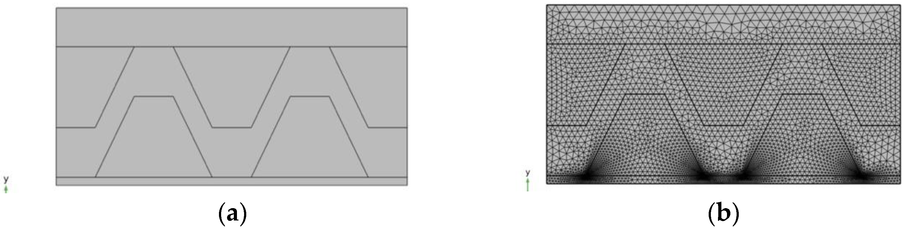
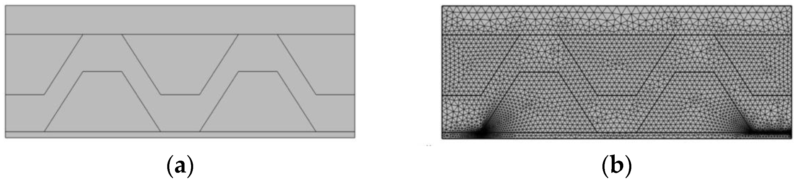
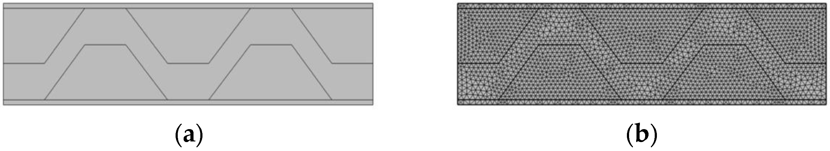
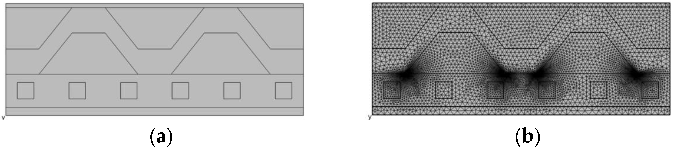
In this work, a three-dimensional finite element method (FEM) model was developed and validated in COMSOL Multiphysics software [19] for the thermal performance assessment of a novel double-skin façade building element. Six geometries were investigated under dynamic conditions. Regarding the domain and mesh of the numerical model, Figure 1, Figure 2, Figure 3, Figure 4, Figure 5 and Figure 6 present the details for the investigated configurations. A physics-controlled mesh and extremely small-sized elements were used to discretize the model, and a time step of 0, 1 and 72 hours was used. The thermophysical properties of the materials used as input for the numerical calculations are presented in Table 2. The numerical simulation geometry dimensions are given in Table 3. The series of the material placement and the dimensions for the six masonry configurations are illustrated in Figure 7, Figure 8 and Figure 9.
2.1. Governing Equations
Under this task, heat transfer in solids was investigated and to this end, the velocity was set to be equal to zero. The equation for pure conductive heat transfer, which was solved for the finite element assessment of this task, was obtained as follows:
In addition, the analysis assumes that mass is always conserved, which means that density and velocity are related through the following equation:
The fundamental law that governs all heat transfer is the first law of thermodynamics, commonly referred to as the principle of conservation of energy. For a fluid subjected to heat transfer, the resulting heat equation is as follows:
The heat transfer interfaces use Fourier’s law of heat conduction, which states that the conductive heat flux, q, is proportional to the temperature gradient, as follows:
The second term on the right of Equation (3) represents the viscous heating of a fluid and the third term quantifies the pressure work and is responsible for the heating of the fluid under adiabatic compression. The last term contains heat sources other than viscous heating.
Inserting Equation (4) into Equation (3), reordering the terms and ignoring viscous heating and pressure work and the other heat sources result in the following equation:
2.2. Boundary Conditions
Concerning the boundary conditions, a temperature profile was assumed on the external surface of the wall and the internal surface of the wall was considered as an open boundary. Considering the exterior wall boundary conditions, the sol-air temperature was implemented. The formula for the calculation of the sol-air temperature Tsol-air is defined as follows:
The analysis was conducted for four calendar months, delivering representative results for the entire calendar year (January—winter, April—spring, July—summer; October—autumn), as well as for the four main orientations (azimuths 0°, 90°, 180° and 270°). The ambient temperature values and the total solar irradiation for Lymbia, Nicosia, Cyprus, were retrieved using the PVGIS tool of JRC [20]. A post-processing analysis of the Tsol-air values was conducted to define the most representative day of the month to be used for the analysis. Particularly, the cumulative standard deviation of each day with the average values of the month was calculated with an hourly time step, and the day of the month with the lowest standard deviation was considered. The standard deviation was calculated as follows:
For the overall heat transfer coefficient ho, the convection and radiation heat transfer coefficients were considered with values of 7.64 and 20, respectively, following the ISO 6946:2017 [21]. The heat exchange with the sky dome was neglected. The calculated hourly temperature values used as boundary conditions are presented in Table 4. Regarding the internal surface temperature of the numerical model, it was assumed to be 22 °C.
2.3. Numerical Model Validation
The validation of the finite element model was considered in this study. For this purpose, a three-dimensional model was developed based on the experimental test cell geometry and the physics employed in this study. The external surface temperatures retrieved from the experimental data were used as the external surface boundary condition and the internal domain was considered as an open boundary. Concerning the methodology of the numerical model validation, the outcome results were compared with the experimental data; specifically, the internal surface temperature was compared against the experimental internal surface temperature. Considering the mesh information of the validation model, the total number of elements was 215,055, with a minimum element quality value of 0.04853, an average element quality value of 0.6518 and a total mesh volume of 0.2469 (m3). The agreement of the experimental (E) and numerical (N) values was calculated with the use of the root mean square deviation (RMSD). The time step of the extracted values was one hour.
2.4. Experimental Setup
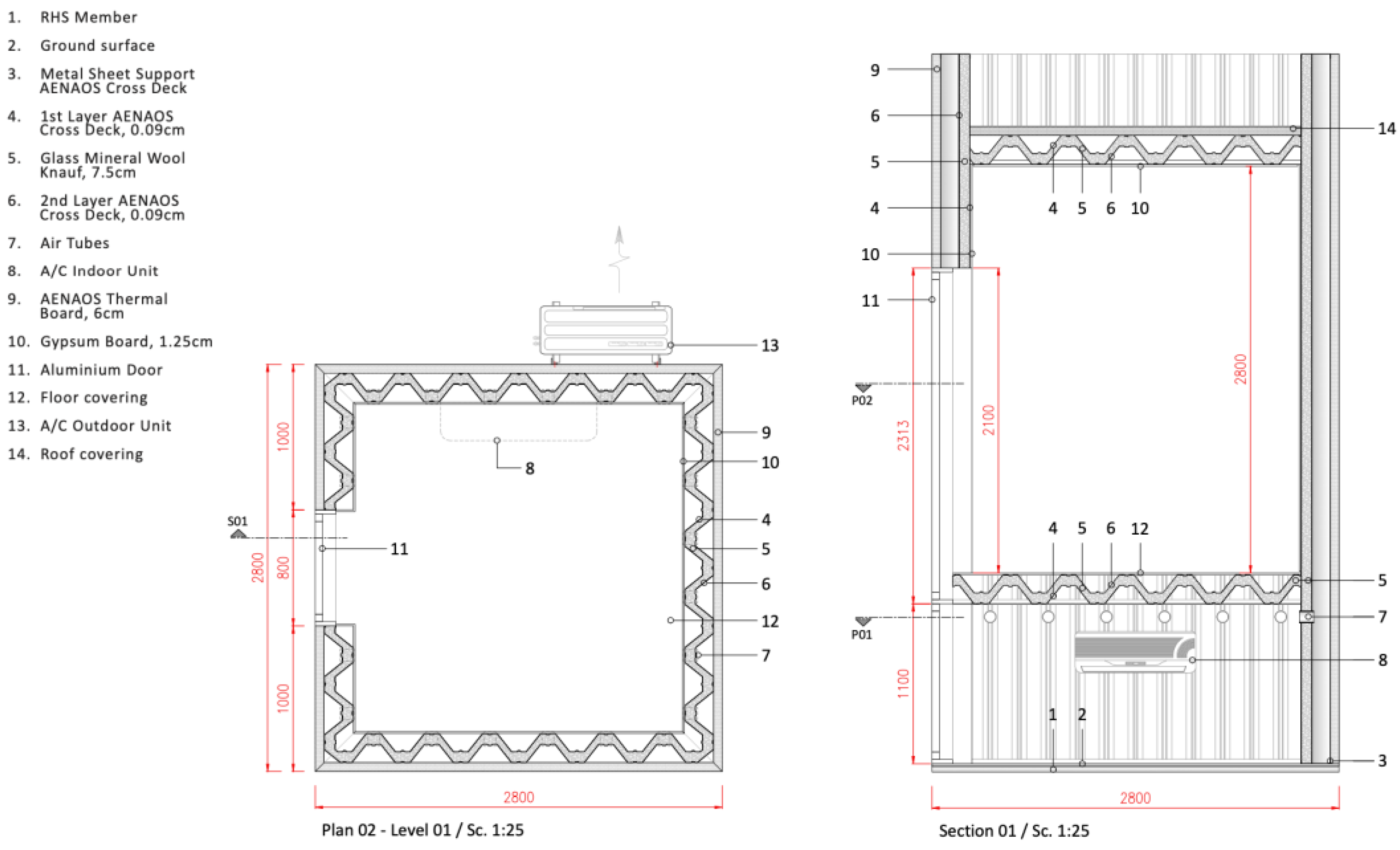
An experimental test cell was constructed in Lymbia, a village in the Nicosia district of Cyprus. Its coordinates are 35°0′0″ (N) and 33°27′45″ (E), with an elevation of 252 m above sea level (see Figure 10). The test cell consists of two floors, with heights of 1.1 m and 2.8 m for the first and second floors, respectively. The test cell width and depth are 2.8 m. Each floor was constructed with an access door with dimensions of 0.8 m × 1.1 m × and 0.8 m × 2.1 m width/height for the first and second floors, respectively. The walls of the construction were built in the material order of the AENAOS thermal board, AENAOS cross deck, glass mineral wool, and gypsum board. The test cell was equipped with an air condition split unit, providing a constant temperature and airflow into integrated air tubes that passed through the wall. In regard to the thickness of the materials and the structure of the test cell, analytical information is presented in Figure 11, Figure 12 and Figure 13.
2.5. Measurement Equipment
Considering the data acquisition process, Table 5 shows the measured parameters and the specifications of the equipment installed in the test cell. The weather station was installed on the roof of the test cell to obtain the ambient temperature, relative humidity, dew point, wind speed, gust speed and direction of the wind. In total, twelve type T thermocouple sensors are installed, with five sensors on the outer and inner faces of the walls, respectively, and one on the inner and outer faces of the top ceiling. Two data loggers, each capable of eight-channel communication, are connected to the sensors. The orientation of the sensor placement is presented in Table 6. The acquisition of the data provided by the weather station and dataloggers is performed at one-hour intervals. The weather station device sends the information to the HOBOlink [22] cloud service where the data are accessible. Regarding the datalogger data, a USB connection is established and the data are extracted from SiteView [23] software via a computer device.
3. Results and Discussion
Figure 14, Figure 15, Figure 16, Figure 17, Figure 18, Figure 19 and Figure 20 present the experimental data for the four calendar months of January, April, July and October. The graphs show the ambient temperature obtained from the weather station and the internal and external measured surface temperatures from the thermocouples for one week for each month.
3.1. Experimental Measurements
3.1.1. Internal Surface Temperature under Winter Conditions
Concerning the thermal performance of the test cell under winter conditions, Figure 14 shows that in January week two, the ambient temperature range was between 5.33 °C and 19.91 °C. The measured data for the internal and external surface temperatures are presented in Figure 15. The lowest internal surface temperature was 19.07 °C for the north-west orientation and the highest was 25.15 °C at the top internal ceiling wall. In regard to the internal surface temperature, a small fluctuation is observed within a range of a maximum of 4.79 °C and the temperature pattern remains mostly constant, even though in certain periods, the temperature difference between the internal and ambient temperature reaches up to 16.57 °C. The data showed that the average internal surface temperature for the January week two period was 22.07 °C.
3.1.2. Internal Surface Temperature under Spring Conditions
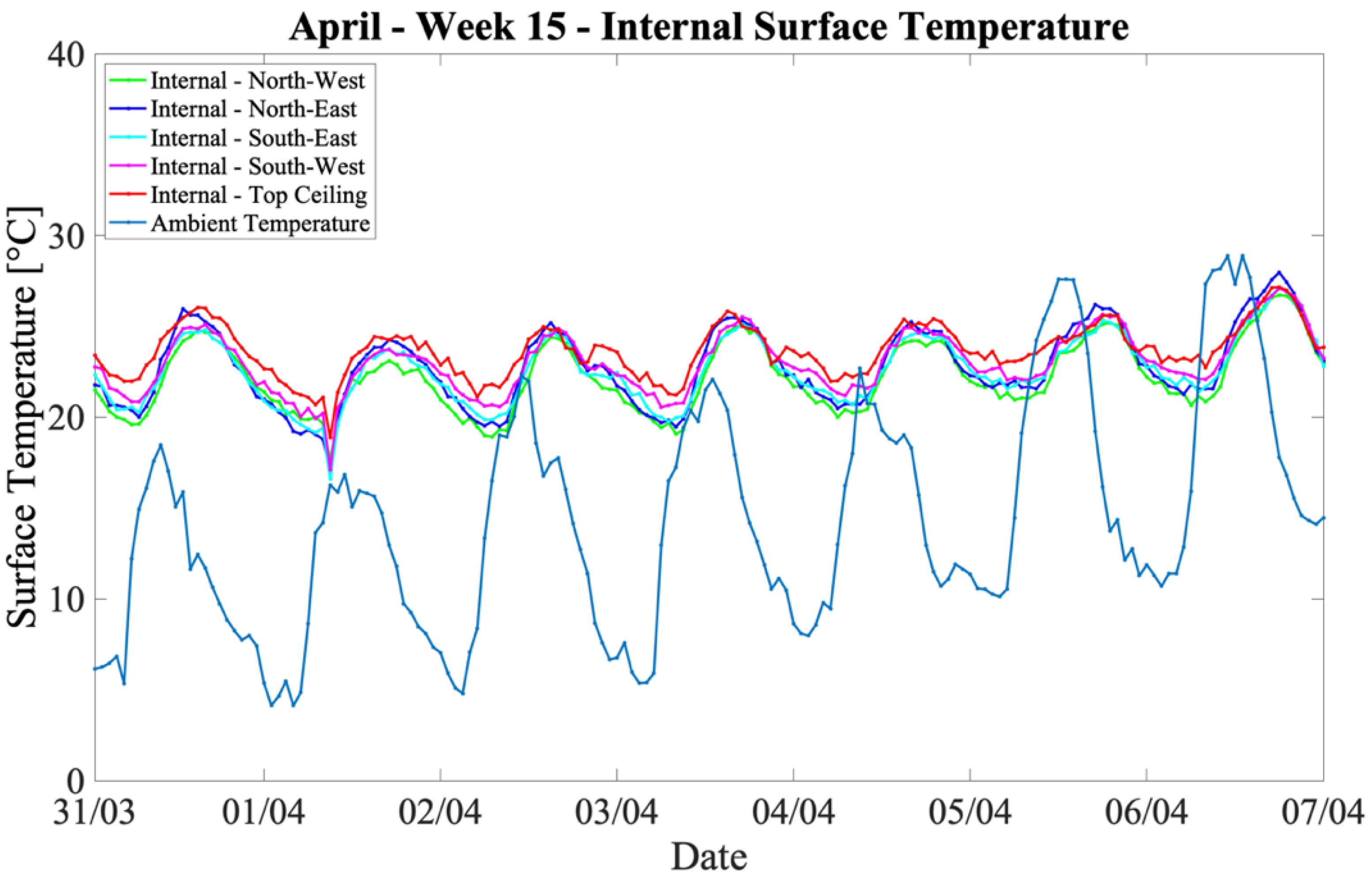
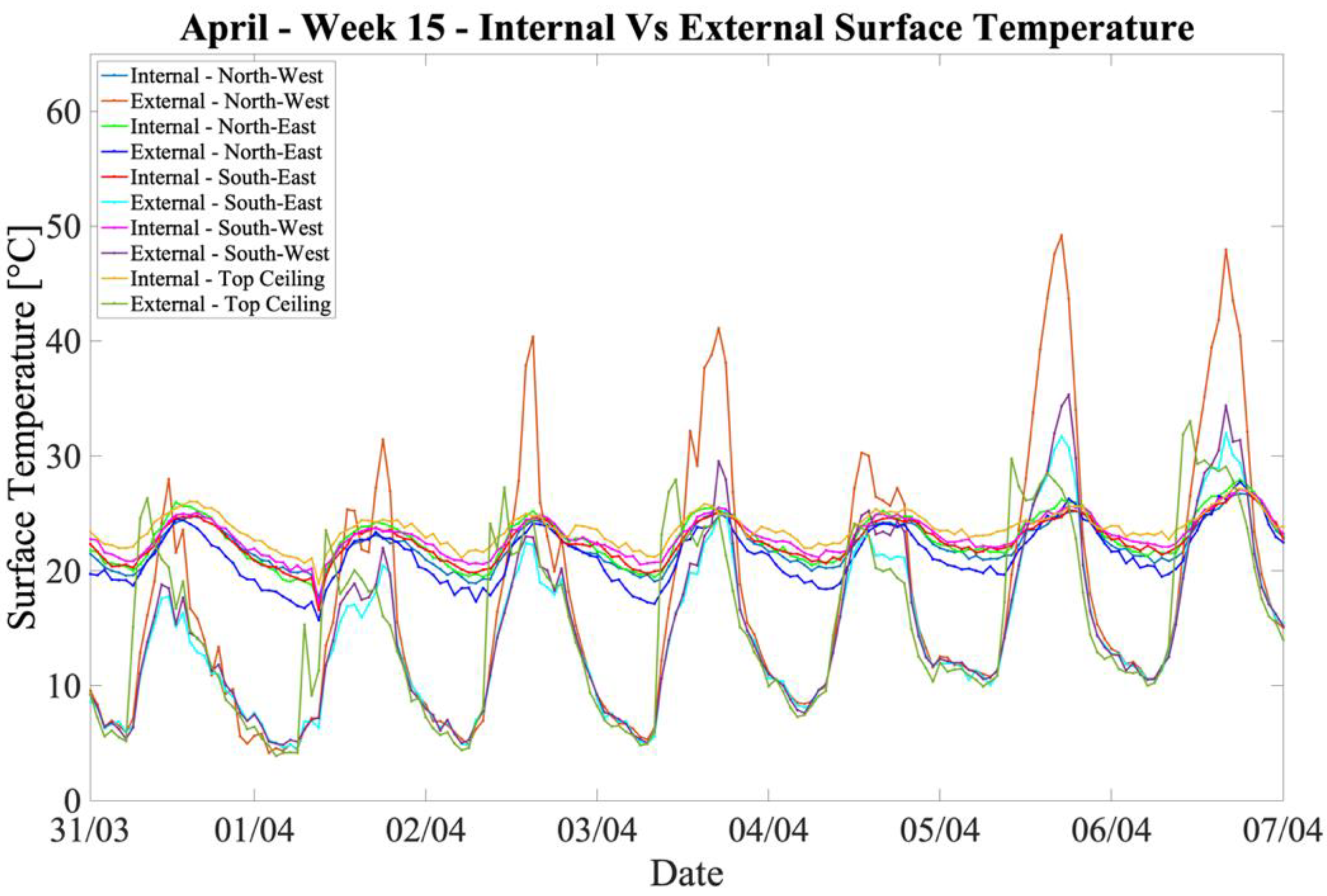
In Figure 16, the experimental data of week fifteen for the April period are presented. It can be observed that there is a considerable fluctuation in the ambient temperature that ranges from 11.32 to 35.56 [°C]. The measured data for the internal and external surface temperatures are presented in Figure 17. The highest internal surface temperature was 27.96 °C for the north-east orientation and the lowest was 16.58 °C for the south-east orientation. The maximum recorded internal surface temperature fluctuation was 10.85 °C for the north-east orientation and the maximum temperature difference between the ambient and internal temperature was 15.54 °C. The average internal surface temperature for the selected period was 22.78 °C.
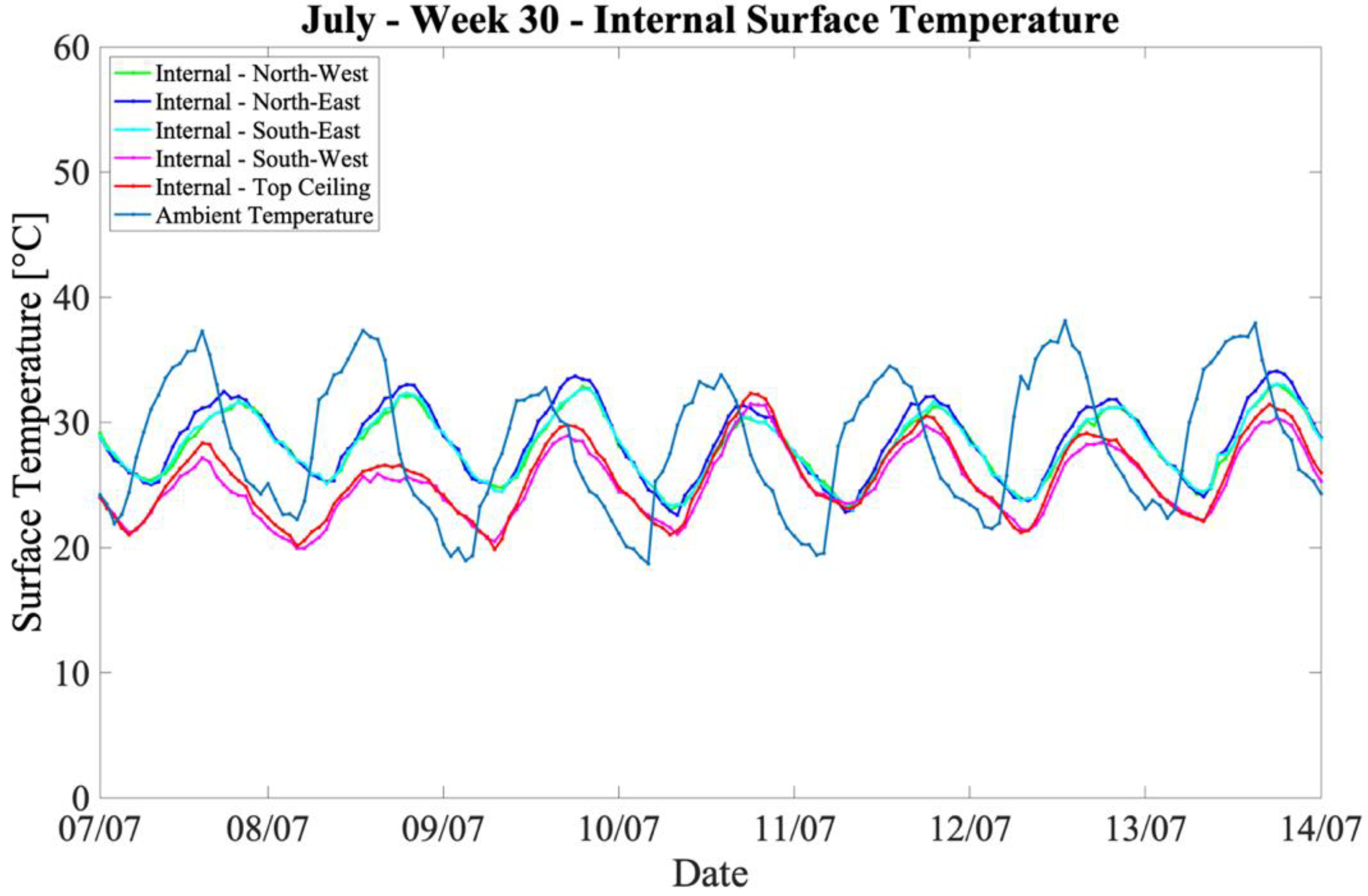
3.1.3. Internal Surface Temperature under Summer Conditions
Figure 18 presents the data for the July period for week thirty. The maximum and minimum ambient temperatures recorded were 37.54 °C and 20.1 °C, respectively. The measured data for the internal and external surface temperatures are presented in Figure 19. The highest internal surface temperature was 36 °C for the north-east orientation and the lowest was 21.09 °C at the internal top ceiling wall. The maximum internal surface temperature fluctuation was 13.52 °C. Considering the comparison between the ambient and internal surface temperature, the data showed a difference of 14.76 °C. According to the obtained data, the average internal surface temperature for July week forty-one was 28.39 °C.
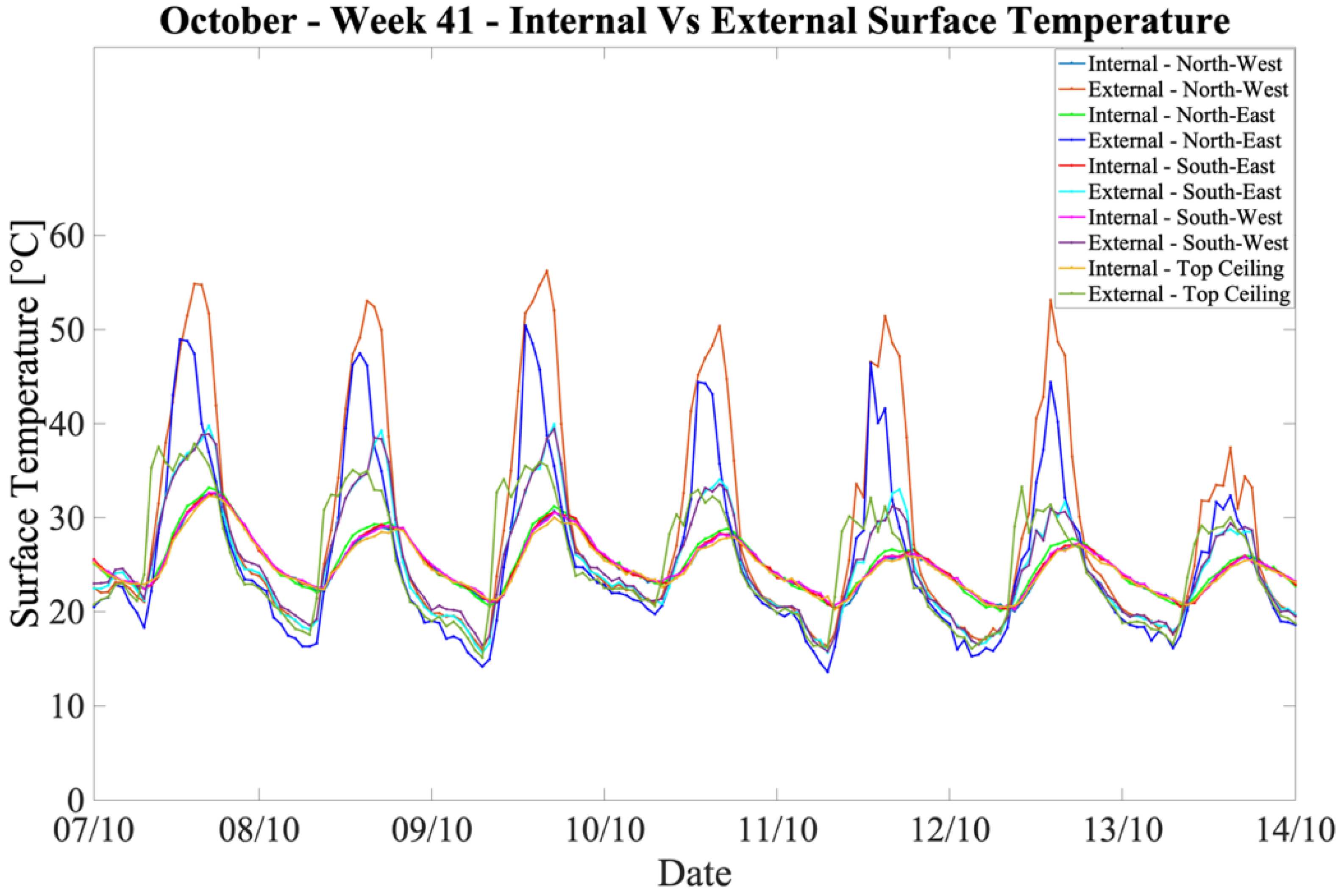
3.1.4. Internal Surface Temperature under Autumn Conditions
Considering the thermal performance of the test cell, Figure 20 presents the experimental data for the October period, week forty-one. It is observed that the lowest and highest ambient temperatures were 15.99 °C and 37.54 °C, respectively. The measured data for the internal and external surface temperatures are presented in Figure 21. The lowest obtained internal surface temperature was 20.07 °C for the north-west orientation and the highest was 33.19 °C for the north-east orientation. The maximum internal surface temperature fluctuation was considered to be 13.1 °C. Comparing the ambient against the internal surface temperature, the maximum difference was 13.01 °C. The overall average internal surface temperature for the selected period was 24.97 °C.
3.2. Numerical Analysis
3.2.1. Numerical Model Validation
The comparison between the experimental data obtained from the test cell and the calculated numerical data indicated that the developed numerical model was accurate and produced reliable results. In Table 7, the calculated RDSM between the experimental and numerical data is presented. It is observed from the comparison of the results that the maximum RDSM value is 3.10 (%) and the lowest is 1.38 (%). The deviation is slightly lower in the case of the north-west orientation and higher for all the other orientations, but remains relatively low. In regard to the percentage deviation for the numerical exercises, 10 (%) and below is considered as acceptable [24].
3.2.2. Thermal Performance under Winter Conditions
In Figure 22, the cumulative daily heat flux values of the investigated geometries under winter conditions are graphically presented. It is observed from the results that geometry five has the worst thermal performance with the highest heat flux value for azimuth 0°. Considering the poor efficiency of geometry five, this probably occurred because the configuration introduced the double-skin façade building element in the internal domain rather than the external domain. The lowest heat flux value was achieved by geometry six for the azimuth 270° orientation, but geometry four was considered to have the best overall thermal performance out of all the structure configurations under winter conditions. Concerning geometry four, azimuth 90° is the ideal orientation to achieve the lowest heat flux value for the winter season.
3.2.3. Thermal Performance under Spring Conditions
The thermal performance of the building element configurations under spring conditions is presented in Figure 23. The calculated heat flux values indicated that the worst thermal performance occurred for geometry five under all orientation scenarios. The lowest heat flux value was achieved by geometry four under the azimuth 180° orientation. Regarding the overall thermal performance geometry, six presented a solid pattern of low heat flux values for all orientations, except azimuth 180°, and was considered to be the best scenario for spring conditions. As observed in the numerical results, the optimum orientation for minimizing thermal losses under spring conditions is the azimuth 180° orientation.
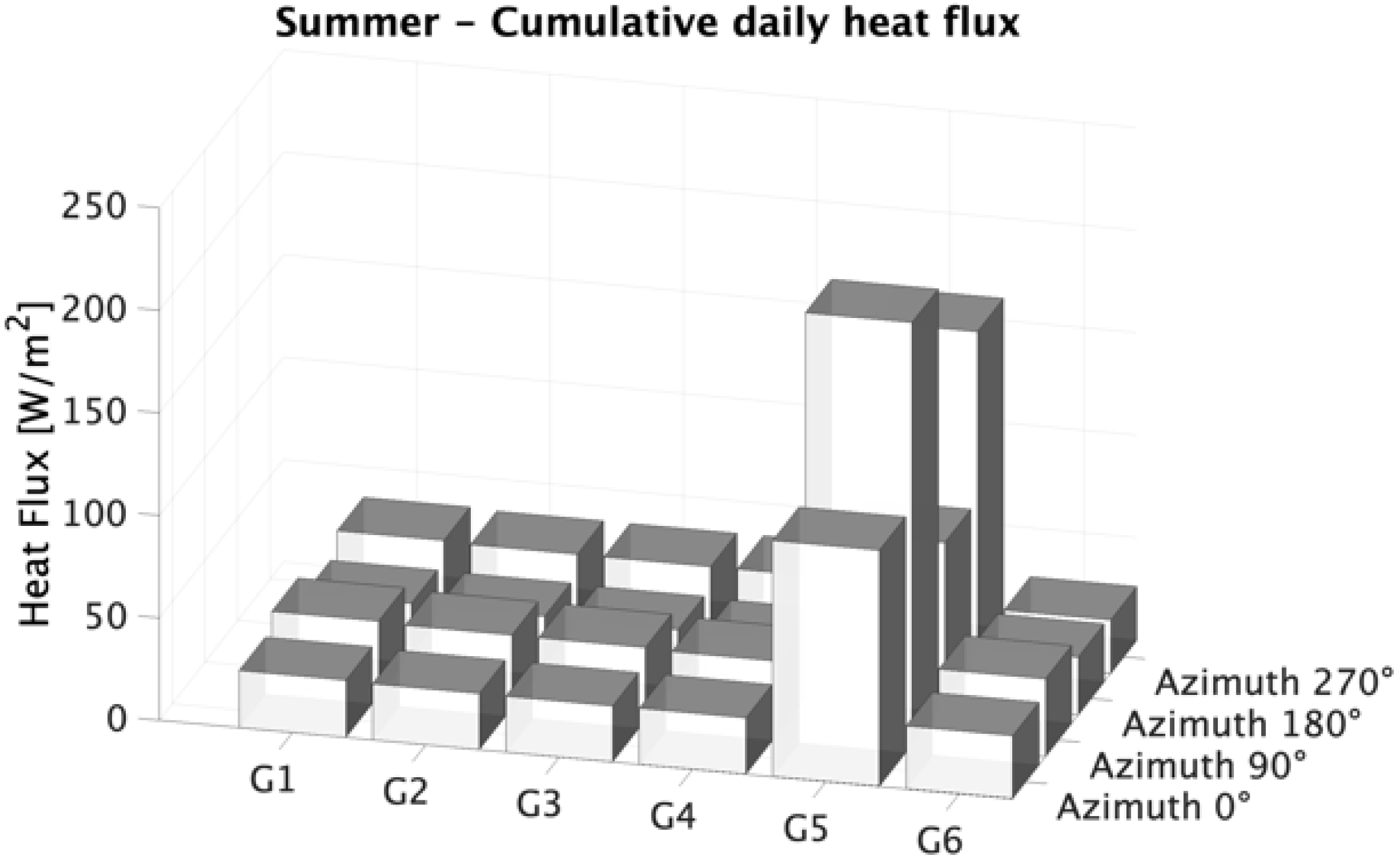
3.2.4. Thermal Performance under Summer Conditions
Figure 24 presents the cumulative heat flux of the investigated configurations under summer conditions. The highest thermal performance of the investigated building element structures was observed in the case of the azimuth 180° orientation for geometry four. The highest cumulative heat flux is observed in geometry five for the azimuth 90° orientation. Based on the numerical findings, the optimal orientation and configuration for the best thermal performance are achieved by geometry four for azimuth 180°.
3.2.5. Thermal Performance under Autumn Conditions
In Figure 25, the cumulative heat flux is presented for the investigated configurations under autumn conditions. It is observed that geometry four and six have the best thermal performance, with the lowest cumulative heat flux through the building element. Geometry five indicated poor thermal performance with the highest cumulative heat flux values. Geometry six for azimuth 90° is distinguished as the optimum scenario and achieved the lowest cumulative heat flux.
3.2.6. Optimal Geometry Analysis
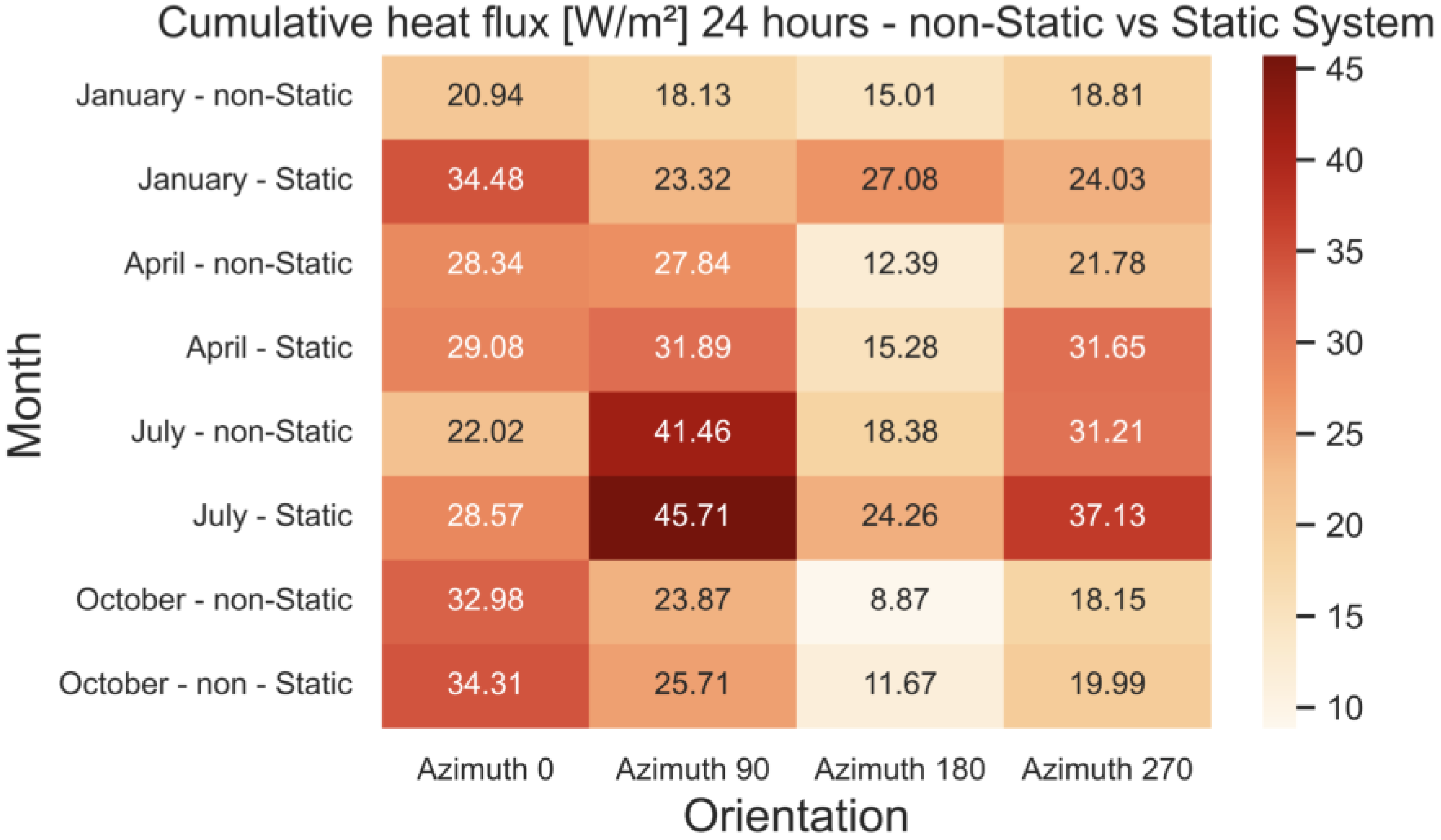
In regard to the thermal performance of the six investigated configurations, geometry four was considered to have the lowest overall heat flux through the masonry. Although the overall thermal performance of geometry four was better, for the construction of the test cell, geometry three was selected because the u-value of geometry four did not meet the minimum requirements. Geometry three was further investigated through the numerical model in regard to the energy difference when the system is non-static versus static. Figure 26 presents the difference in cumulative heat flux for 24 h through the masonry. Based on the numerical calculation, the cumulative heat flux is less when the air circulation is active through the masonry versus being static. In Figure 27 and Figure 28, the total energy savings in kWh/m2 and % are presented for the non-static versus the static system. The annual total energy savings in kWh/m2 were 1.99, 1.38, 2.13 and 2.06 for azimuth 0°, 90°, 180° and 270°, respectively. In regard to the total energy savings in %, the maximum benefit was considered to be in the winter season, with values of 65, 29, 80 and 28 for azimuth 0°, 90°, 180° and 270°, respectively.
4. Conclusions
This study investigated a novel controlled-temperature double-skin façade (DSF) building element with controlled-temperature air and flow to achieve a “thermal barrier” through the building envelope. The external and internal surface temperature and ambient conditions were measured. A numerical investigation based on six developed geometries was performed and the finite element model used was validated with the use of experimental data obtained from the constructed test cell. Based on the numerical investigation results, the continuous supply of controlled air temperature and flow through the building masonry revealed the building’s improved thermal performance by reducing the cumulative heat flux, resulting in annual total energy savings in kWh/m2 of 1.99, 1.38, 2.13 and 2.06 for azimuth 0°, 90°, 180° and 270°, respectively. In regard to the total energy savings in %, the maximum benefit was considered to be in the winter season, with values of 65, 29, 80 and 28 for azimuth 0°, 90°, 180° and 270°, respectively. In addition, the controlled-temperature air with a constant flow showed the test cell’s ability to absorb and release heat under hot and cold conditions, respectively. Based on the experimental measurements, the internal surface temperature remained constant, with small fluctuations under diverse conditions. Conclusively, the study findings indicated that the internal surface temperature of the building envelope was not significantly affected by the building orientation, revealing its tolerance to ambient condition changes. The controlled-temperature double-skin façade (DSF) building element can potentially provide viable solutions to the building industry for better thermal performance, contributing to the reduction in energy consumption for the building sector.
Author Contributions
L.G.: Formal analysis, Investigation; Writing—Review and Editing. N.A. Measurements, Data Curation, Data Post-processing, Visualization P.A.F.: Conceptualization, Methodology, Validation, Resources, Supervision; Project administration. All authors have read and agreed to the published version of the manuscript.
Funding
This research was funded by the Ministry of Energy, Commerce, Industry and Tourism, Republic of Cyprus, under the “Sustainable Development and Competitiveness. Development of Innovative Products, Services and Processes” funding program (Project Protocol No. 8.1.12.13.3.154).
Data Availability Statement
The data presented in this study are openly available at Mendeley Data (https://0-doi-org.brum.beds.ac.uk/10.17632/dfj4f7fww4.4 (accessed on 1 January 2023)).
Acknowledgments
This work is a part of the dissemination activities of the research project “Design and Development of the “Controlled Temperature Building Shell” concept (AENAOS)”.
Conflicts of Interest
The authors declare that they have no known competing financial interests or personal relationships that have, or could be perceived to have, influenced the work reported in this article.
References
- Barbosa, S.; Ip, K. Perspectives of double skin façades for naturally ventilated buildings: A review. Renew. Sustain. Energy Rev. 2014, 40, 1019–1029. [Google Scholar] [CrossRef]
- Aldawoud, A.; Salameh, T.; Ki Kim, Y. Double skin façade: Energy performance in the United Arab Emirates. Energy Sources Part B Econ. Plan. Policy 2021, 16, 387–405. [Google Scholar] [CrossRef]
- Barbosa, S.; Ip, K. Predicted thermal acceptance in naturally ventilated office buildings with double skin façades under Brazilian climates. J. Build. Eng. 2016, 7, 92–102. [Google Scholar] [CrossRef]
- Catto Lucchino, E.; Gelesz, A.; Skeie, K.; Gennaro, G.; Reith, A.; Serra, V.; Goia, F. Modelling double skin façades (DSFs) in whole-building energy simulation tools: Validation and inter-software comparison of a mechanically ventilated single-story DSF. Build. Environ. 2021, 199, 107906. [Google Scholar] [CrossRef]
- Chan, A.L.S.; Chow, T.T. Calculation of overall thermal transfer value (OTTV) for commercial buildings constructed with naturally ventilated double skin façade in subtropical Hong Kong. Energy Build. 2014, 69, 14–21. [Google Scholar] [CrossRef]
- Norouzi, R.; Motalebzade, R. Effect of Double-Skin Façade on Thermal Energy Losses in Buildings, in Exergetic, Energetic and Environmental Dimensions; Elsevier: Amsterdam, The Netherlands, 2018; pp. 193–209. [Google Scholar] [CrossRef]
- Qahtan, A.M. Thermal performance of a double-skin façade exposed to direct solar radiation in the tropical climate of Malaysia: A case study. Case Stud. Therm. Eng. 2019, 14, 100419. [Google Scholar] [CrossRef]
- Radmard, H.; Ghadamian, H.; Esmailie, F.; Ahmadi, B.; Adl, M. Examining a numerical model validity for performance evaluation of a prototype solar oriented Double skin Façade: Estimating the technical potential for energy saving. Sol. Energy 2020, 211, 799–809. [Google Scholar] [CrossRef]
- Tao, Y.; Zhang, H.; Huang, D.; Fan, C.; Tu, J.; Shi, L. Ventilation performance of a naturally ventilated double skin façade with low-E glazing. Energy 2021, 229, 120706. [Google Scholar] [CrossRef]
- Souza, L.C.O.; Souza, H.A.; Rodrigues, E.F. Experimental and numerical analysis of a naturally ventilated double-skin façade. Energy Build. 2018, 165, 328–339. [Google Scholar] [CrossRef]
- Góes, T.; Silva, C.F. Hybrid double-skin façade: Thermal and energy performance in Brasília, Brazil. In Proceedings of the SB-LAB 2017—International Conference on Advances on Sustainable Cities and Buildings Development, Porto, Portugal, 15–17 November 2017. [Google Scholar]
- Tao, Y.; Zhang, H.; Zhang, L.; Zhang, G.; Tu, J.; Shi, L. Ventilation performance of a naturally ventilated double-skin façade in buildings. Renew. Energy 2021, 167, 184–198. [Google Scholar] [CrossRef]
- Anđelković, A.S.; Mujan, I.; Dakić, S. Experimental validation of an EnergyPlus model: Application of a multi-storey naturally ventilated double skin façade. Energy Build. 2016, 118, 27–36. [Google Scholar] [CrossRef]
- de María, J.M.; Bravo, A.; Camarasa, M.; Pern’ia, E.; Baïri, A.; Laraqi, N. Thermal and energy analysis of double-skin façades. In Proceedings of the 9th International Conference on Heat Transfer, Fluid Mechanics and Thermodynamics, St. Julians, Malta, 16–18 July 2012. [Google Scholar]
- Iken, O.; Fertahi, S.D.; Dlimi, M.; Agounoun, R.; Kadiri, I.; Sbai, K. Thermal and energy performance investigation of a smart double skin facade integrating vanadium dioxide through CFD simulations. Energy Convers. Manag. 2019, 195, 650–671. [Google Scholar] [CrossRef]
- Lee, S.W.; Park, J.S. Evaluating the thermal performance of double-skin facade using response factor. Energy Build. 2020, 209, 109657. [Google Scholar] [CrossRef]
- Wang, Y.; Chen, Y.; Zhou, J. Dynamic modelling of the ventilated double skin façade in hot summer and cold winter zone in China. Build. Environ. 2016, 106, 365–377. [Google Scholar] [CrossRef]
- Sanchez, E.; Rolando, A.; Sant, R.; Ayuso, L. Influence of natural ventilation due to buoyancy and heat transfer in the energy efficiency of a double skin facade building. Energy Sustain. Dev. 2016, 33, 139–148. [Google Scholar] [CrossRef]
- COMSOL Multiphysics. Available online: https://www.comsol.com/comsol-multiphysics (accessed on 15 December 2022).
- PVGIS Photovoltaic Geographical Information System. Available online: https://joint-research-centre.ec.europa.eu/pvgis-photovoltaic-geographical-information-system_en (accessed on 15 December 2022).
- ISO 6946:2017. Building Components and Building Elements—Thermal Resistance and Thermal Transmittance—Calculation Methods. Available online: https://www.iso.org/standard/65708.html (accessed on 15 December 2022).
- HOBOlink. Available online: https://www.onsetcomp.com/products/software/hobolink/ (accessed on 15 December 2022).
- SiteView. Available online: https://www.microedgeinstruments.com/siteview.php (accessed on 15 December 2022).
- Pawar, V.R.; Sobhansarbandi, S. CFD modelling of a thermal energy storage-based heat pipe evacuated tube solar collector. J. Energy Storage 2020, 30, 101528. [Google Scholar] [CrossRef]
Figure 1.
(a) Geometry One Configuration; (b) Geometry One Domain Mesh.

Figure 2.
(a) Geometry Two Configuration; (b) Geometry Two Domain Mesh.

Figure 3.
(a) Geometry Three Configuration; (b) Geometry Three Domain Mesh.

Figure 4.
(a) Geometry Four Configuration; (b) Geometry Four Domain Mesh.

Figure 5.
(a) Geometry Five Configuration; (b) Geometry Five Domain Mesh.

Figure 6.
(a) Geometry Six Configuration; (b) Geometry Six Domain Mesh.

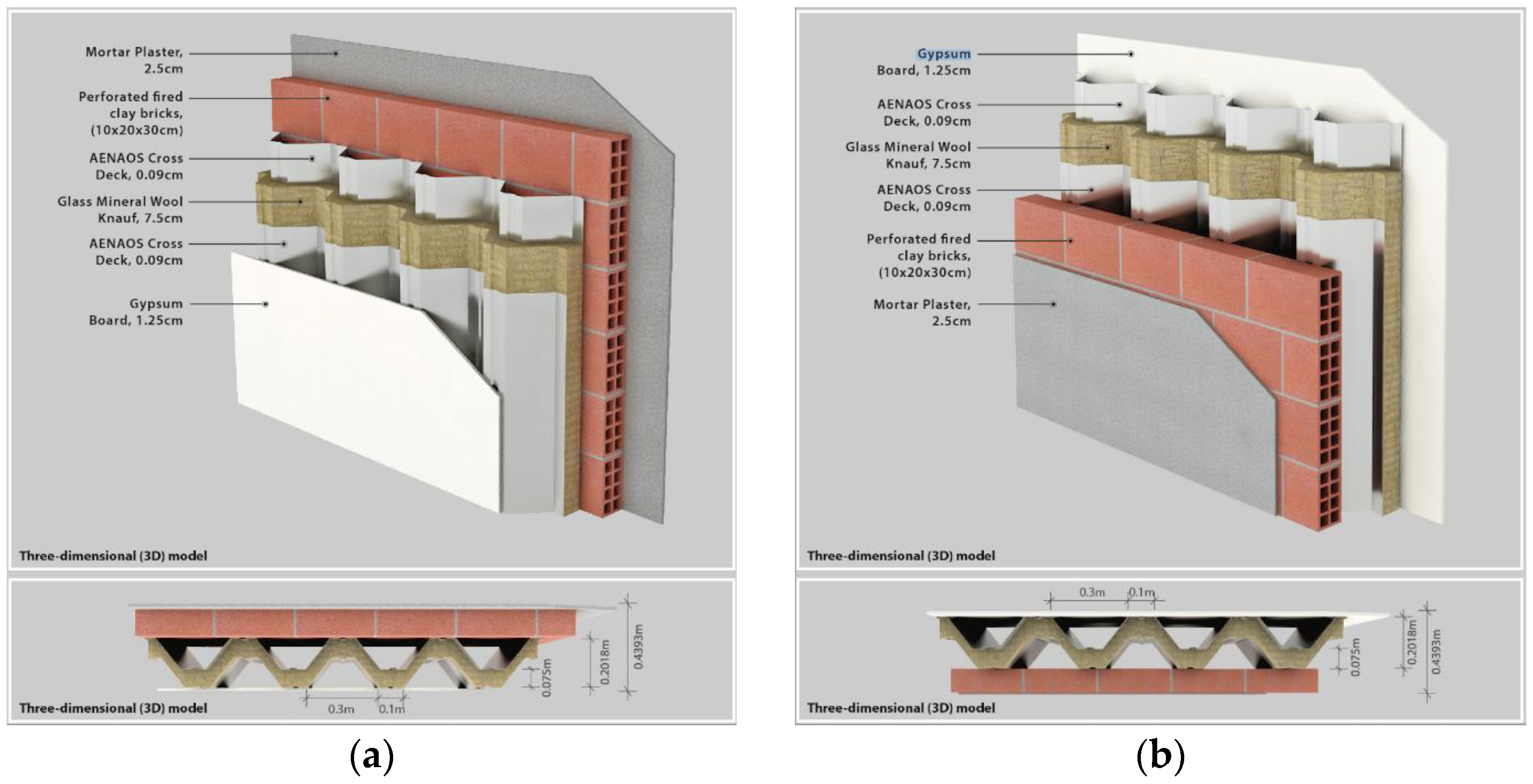
Figure 7.
(a) Configuration One—Geometry Dimensions and Materials; (b) Configuration Two—Geometry Dimensions and Materials.
Figure 7.
(a) Configuration One—Geometry Dimensions and Materials; (b) Configuration Two—Geometry Dimensions and Materials.

Figure 8.
(a) Configuration Three—Geometry Dimensions and Materials; (b) Configuration Four—Geometry Dimensions and Materials.
Figure 8.
(a) Configuration Three—Geometry Dimensions and Materials; (b) Configuration Four—Geometry Dimensions and Materials.

Figure 9.
(a) Configuration Five—Geometry Dimensions and Materials; (b) Configuration Six—Geometry Dimensions and Materials.
Figure 9.
(a) Configuration Five—Geometry Dimensions and Materials; (b) Configuration Six—Geometry Dimensions and Materials.

Figure 10.
(a) Experimental Test Cell; (b) Experimental Test Cell—First and Second Level.

Figure 11.
Test Cell—Cross Section View One.

Figure 12.
Test Cell—Cross Section View Two.

Figure 13.
Test Cell—Cross Section View Three.

Figure 14.
Internal Surface Temperature vs. Ambient Temperature—January—Week 2.

Figure 15.
Internal vs. External Surface Temperature—January—Week 2.

Figure 16.
Internal Surface Temperature vs. Ambient Temperature—April—Week 15.

Figure 17.
Internal vs. External Surface Temperature–April—Week 15.

Figure 18.
Internal Surface Temperature vs. Ambient Temperature—July—Week 30.

Figure 19.
Internal vs. External Surface Temperature—July—Week 30.

Figure 20.
Internal Surface Temperature vs. Ambient Temperature—October—Week 41.

Figure 21.
Internal vs. External Surface Temperature—October—Week 41.

Figure 22.
Cumulative Daily Heat Flux—Winter—Geometry 1 to 6—All Orientations.

Figure 23.
Cumulative Daily Heat Flux—Spring—Geometry 1 to 6—All Orientations.

Figure 24.
Cumulative daily heat flux—Summer—Geometry 1 to 6—All Orientations.

Figure 25.
Cumulative daily heat flux—Autumn—Geometry 1 to 6—All Orientations.

Figure 26.
Cumulative Heat Flux (W/m2)—24 h—Non-Static vs. Static System.

Figure 27.
Total Energy Saving (kWh/m2yr)—Non-Static vs. Static System.

Figure 28.
Total Energy Saving (%)—Non-Static vs. Static System.


Table 1.
Investigation study characteristics.
| Study | Software | Location | Analysis Type | Solar Radiation (W/m2) | Ambient Temperature (°C) | Wind Speed (m/s) | Cavity Depth (m) | Study Results |
|---|---|---|---|---|---|---|---|---|
| [9] | ANSYS Fluent | - | Numerical Model | 50–1000 | - | - | 0.1–0.4 | Glazing Inner/Outer Temperature (°C); Incident Radiation (W/m2) |
| [4] | Energy Plus, TRNSYS, IDA ICE, IES-VE | Italy | Test Cell | Dynamic Profile | Dynamic Profile | - | 0.24 | Heat Flux (W/m2), Surface Temperature (°C); Total Energy (kWh/m2) |
| [8] | MATLAB | Iran | Existing Building/Numerical Model | - | - | - | 0.3 | Temperature across DSF (°C); Cooling Energy Consumption (kW/h) |
| [16] | TRNSYS | Korea | Test Cell | Dynamic Profile | Dynamic Profile | 2.7 | - | Surface Temperature (°C), Sensible Cooling Load (kW); Cooling Energy Consumption (kW/h) |
| [7] | - | Malaysia | Existing Building | Dynamic Profile | Dynamic Profile | 0–0.1 | 1.2 | Air Temperature (Indoor/Outdoor) (°C), Solar Radiation (W/m2); Air Velocity in DSF (m/s) |
| [15] | - | Morocco | Numerical Model | Dynamic Profile | Dynamic Profile | Dynamic Profile | - | Temperature across DSF (°C); Air Velocity in DSF (m/s) |
| [12] | ANSYS Fluent | - | Numerical Model | 740 | 20 | - | - | Surface Temperature (°C), Temperature of Inner DSF Face (°C); Air Velocity in DSF (m/s) |
| [10] | ANSYS CFX | Brazil | Test Cell/Numerical Model | Dynamic Profile | Dynamic Profile | - | - | Test Cell Inner/Outer Face Temperature (°C); Air Velocity in DSF (m/s) |
| [11] | Energy Plus, Design builder | Brazil | Numerical Model | Dynamic Profile | Dynamic Profile | - | - | Building Energy Consumption (kW/h) |
| [2] | Energy Plus, Design builder | UAE | Numerical Model | - | Dynamic Profile | Dynamic Profile | 0.6 and 1.2 | Glazing Inner/Outer Temperature (°C); Wall Inner/Outer Temperature (°C) |
| [14] | ANSYS Fluent | - | Test Cell/Numerical Model | Dynamic Profile | Dynamic Profile | - | - | Heat Flux (W/m2), DSF Inner/Outer Temperature (°C); Wall Temperature (°C) |
| [5] | Energy Plus | China | Numerical Model | - | 22 | - | 0.2–1 | Glazing Inner/Outer Temperature (°C) |
| [17] | - | China | Test Cell/Numerical Model | Dynamic Profile | - | - | - | Surface Temperature (°C) |
| [3] | IESVE | Brazil | Numerical Model | Dynamic Profile | Dynamic Profile | - | 1 | Air Velocity in DSF (m/s) |
| [18] | ANSYS Fluent | Spain | Numerical Model | Dynamic Profile | 4–32 | - | - | Heat Flux (W/m2) |
| [6] | Design builder | Iran | Test Cell/Numerical Model | Dynamic Profile | Dynamic Profile | - | Variable | Sensible Heating Load (kWh) |
| [13] | Energy Plus, Design builder | Serbia | Existing Building/Numerical Model | Dynamic Profile | Dynamic Profile | Dynamic Profile | - | Cavity Air Temperature (°C) |
Table 2.
Thermophysical properties of the materials used as input in the numerical simulation study of novel double-skin façade (DSF) controlled-temperature building element.
Table 2.
Thermophysical properties of the materials used as input in the numerical simulation study of novel double-skin façade (DSF) controlled-temperature building element.
| Material | Density (Kg/m3) | Thermal Conductivity (W/(m∙K)) | Heat Capacity (J(Kg∙K)) | Thickness (cm) |
|---|---|---|---|---|
| Glass Mineral Wool | 50 | 0.04 | 1030 | 7.50 |
| Gypsum Board | 664 | 0.19 | 1090 | 1.25 |
| Mortar Plaster | 700 | 1 | 1000 | 2.50 |
| Perforated Fired Clay Brick (Clay Material) | 880 | 0.4 | 900 | 20 |
| Perforated Fired Clay Brick (Air Holes 5 × 5 (cm)) | 1.23 | 0.025 | 1008 | 20 |
| AENAOS Cross Deck | 7850 | 44.5 | 475 | 0.09 |
| AENAOS Thermal Board | 400 | 0.104 | 900 | 6 |
Table 3.
Numerical simulation geometry dimensions.
| Geometry | Height (m) | Width (m) | Air Tube Height (m) |
|---|---|---|---|
| G1 | 0.2743 | 0.54 | 0.125 |
| G2 | 0.2743 | 0.72 | 0.125 |
| G3 | 0.2743 | 0.9 | 0.125 |
| G4 | 0.2493 | 0.9 | 0.125 |
| G5 | 0.3393 | 0.9 | 0.125 |
| G6 | 0.3393 | 0.9 | 0.125 |
Table 4.
Calculated hourly temperature values used as external boundary temperature (°C) in the numerical simulation study of novel double-skin façade (DSF) controlled-temperature building element.
Table 4.
Calculated hourly temperature values used as external boundary temperature (°C) in the numerical simulation study of novel double-skin façade (DSF) controlled-temperature building element.
| Winter | Spring | Summer | Autumn | |||||||||||||
|---|---|---|---|---|---|---|---|---|---|---|---|---|---|---|---|---|
| Time (hour) | Azimuth (°) | |||||||||||||||
| 0 | 90 | 180 | 270 | 0 | 90 | 180 | 270 | 0 | 90 | 180 | 270 | 0 | 90 | 180 | 270 | |
| 1 | 12.01 | 12.01 | 12.01 | 12.01 | 15.66 | 15.66 | 15.66 | 15.66 | 25.84 | 25.84 | 25.84 | 25.84 | 23.74 | 23.74 | 23.74 | 23.74 |
| 2 | 12.01 | 12.01 | 12.01 | 12.01 | 15.57 | 15.57 | 15.57 | 15.57 | 25.52 | 25.52 | 25.52 | 25.52 | 23.66 | 23.66 | 23.66 | 23.66 |
| 3 | 12.01 | 12.01 | 12.01 | 12.01 | 15.47 | 15.47 | 15.47 | 15.47 | 25.20 | 25.20 | 25.20 | 25.20 | 23.58 | 23.58 | 23.58 | 23.58 |
| 4 | 12.02 | 12.02 | 12.02 | 12.02 | 15.38 | 15.38 | 15.38 | 15.38 | 25.07 | 25.07 | 25.60 | 26.12 | 23.49 | 23.49 | 23.49 | 23.49 |
| 5 | 12.14 | 12.14 | 12.14 | 12.14 | 16.96 | 16.96 | 18.29 | 25.61 | 27.17 | 27.17 | 31.48 | 40.21 | 23.98 | 23.79 | 23.79 | 24.72 |
| 6 | 12.66 | 12.32 | 12.32 | 12.25 | 20.30 | 18.50 | 18.78 | 35.59 | 28.55 | 28.55 | 32.77 | 49.87 | 30.15 | 24.97 | 24.97 | 37.42 |
| 7 | 20.63 | 13.41 | 13.41 | 13.12 | 25.58 | 19.93 | 19.93 | 39.18 | 30.93 | 29.66 | 30.99 | 52.21 | 35.61 | 25.87 | 25.87 | 40.78 |
| 8 | 24.84 | 14.52 | 14.52 | 23.30 | 30.45 | 20.91 | 20.91 | 38.88 | 35.47 | 30.18 | 30.18 | 49.86 | 41.08 | 26.92 | 26.92 | 40.84 |
| 9 | 30.47 | 15.30 | 15.30 | 24.32 | 33.99 | 22.07 | 22.07 | 34.81 | 38.61 | 30.48 | 30.48 | 45.14 | 44.94 | 28.24 | 28.24 | 37.89 |
| 10 | 32.67 | 15.68 | 15.68 | 24.46 | 35.82 | 22.38 | 22.38 | 28.97 | 40.59 | 30.82 | 30.82 | 38.66 | 46.92 | 28.97 | 28.97 | 33.10 |
| 11 | 31.93 | 17.93 | 15.69 | 20.89 | 35.26 | 27.80 | 23.05 | 23.05 | 40.92 | 35.72 | 30.98 | 30.98 | 44.83 | 34.60 | 29.59 | 29.59 |
| 12 | 30.29 | 21.87 | 15.76 | 15.91 | 33.68 | 33.08 | 22.74 | 22.74 | 39.82 | 42.78 | 31.11 | 31.11 | 42.51 | 38.06 | 28.83 | 28.83 |
| 13 | 27.59 | 24.38 | 15.84 | 15.98 | 30.57 | 36.62 | 22.06 | 22.06 | 37.24 | 47.31 | 31.26 | 31.26 | 40.44 | 41.56 | 28.79 | 28.79 |
| 14 | 24.57 | 25.38 | 15.09 | 15.65 | 27.61 | 39.27 | 21.83 | 21.83 | 34.13 | 51.15 | 30.89 | 30.89 | 35.30 | 40.48 | 27.86 | 27.86 |
| 15 | 18.25 | 20.67 | 14.04 | 14.90 | 23.69 | 40.13 | 20.93 | 20.93 | 30.26 | 53.52 | 32.88 | 30.26 | 30.02 | 35.63 | 26.68 | 26.68 |
| 16 | 13.26 | 13.26 | 13.26 | 13.85 | 20.11 | 34.18 | 21.13 | 20.01 | 29.83 | 50.48 | 34.60 | 29.83 | 25.35 | 25.35 | 25.35 | 25.35 |
| 17 | 13.20 | 13.20 | 13.20 | 13.20 | 18.13 | 18.20 | 18.16 | 18.13 | 28.72 | 40.99 | 33.19 | 28.72 | 24.98 | 24.98 | 24.98 | 24.98 |
| 18 | 13.14 | 13.14 | 13.14 | 13.14 | 17.46 | 17.46 | 17.46 | 17.46 | 27.60 | 27.60 | 27.60 | 27.60 | 24.62 | 24.62 | 24.62 | 24.62 |
| 19 | 13.07 | 13.07 | 13.07 | 13.07 | 16.80 | 16.80 | 16.80 | 16.80 | 27.24 | 27.24 | 27.24 | 27.24 | 24.26 | 24.26 | 24.26 | 24.26 |
| 20 | 13.07 | 13.07 | 13.07 | 13.07 | 16.52 | 16.52 | 16.52 | 16.52 | 26.83 | 26.83 | 26.83 | 26.83 | 24.00 | 24.00 | 24.00 | 24.00 |
| 21 | 13.07 | 13.07 | 13.07 | 13.07 | 16.24 | 16.24 | 16.24 | 16.24 | 26.42 | 26.42 | 26.42 | 26.42 | 23.74 | 23.74 | 23.74 | 23.74 |
| 22 | 13.07 | 13.07 | 13.07 | 13.07 | 15.95 | 15.95 | 15.95 | 15.95 | 26.01 | 26.01 | 26.01 | 26.01 | 23.49 | 23.49 | 23.49 | 23.49 |
| 23 | 13.47 | 13.47 | 13.47 | 13.47 | 15.96 | 15.96 | 15.96 | 15.96 | 25.82 | 25.82 | 25.82 | 25.82 | 23.45 | 23.45 | 23.45 | 23.45 |
| 24 | 13.87 | 13.87 | 13.87 | 13.87 | 15.97 | 15.97 | 15.97 | 15.97 | 25.64 | 25.64 | 25.64 | 25.64 | 23.41 | 23.41 | 23.41 | 23.41 |
Table 5.
Equipment device specifications and measured parameters.
| Parameters Measured | Unit | Model | Sensor | Description |
|---|---|---|---|---|
| Relative Humidity | (%) | S-THB-M002 | Temp/RH Sensor (12bit) | Onset HOBO RX3002 Wi-Fi Remote Monitoring Station |
| Ambient Temperature | (°C) | |||
| Dew Point | (°C) | |||
| Wind Speed | (m/s) | S-WCF-M002 | Davis® Wind Speed and Direction | |
| Gust Speed | (m/s) | |||
| Wind Direction | (°) | |||
| Solar Radiation | (W/m2) | S-LIB-M003 | Silicon Pyranometer | |
| Surface Temperature—Twall (Inner/Outer) | (°C) | S-LIB-M003 | Thermocouple T-type | Thermocouple Datalogger |
Table 6.
Thermocouple type T placement orientation.
| T1: North-West Internal | T7: South-East Internal |
| T2: North-West External | T8: South-East External |
| T3: North-West Internal | T9: South-West Internal |
| T4: North-West External | T10: South-West External |
| T5: North-East Internal | T11: Top Ceiling—Internal |
| T6: North-East External | T12: Top Ceiling—External |
Table 7.
RMSD of experimental and numerical values for FE model validation.
| Month | Orientation | |||
|---|---|---|---|---|
| North-West | North-East | South-East | South-West | |
| January | 1.54 (%) | 1.40 (%) | 2.59 (%) | 2.96 (%) |
| August | 1.38 (%) | 3.10 (%) | 2.79 (%) | 2.68 (%) |
Disclaimer/Publisher’s Note: The statements, opinions and data contained in all publications are solely those of the individual author(s) and contributor(s) and not of MDPI and/or the editor(s). MDPI and/or the editor(s) disclaim responsibility for any injury to people or property resulting from any ideas, methods, instructions or products referred to in the content. |
© 2023 by the authors. Licensee MDPI, Basel, Switzerland. This article is an open access article distributed under the terms and conditions of the Creative Commons Attribution (CC BY) license (https://creativecommons.org/licenses/by/4.0/).
Share and Cite
MDPI and ACS Style
Georgiou, L.; Afxentiou, N.; Fokaides, P.A. Numerical Investigation of a Novel Controlled-Temperature Double-Skin Façade (DSF) Building Element. Energies 2023, 16, 1836. https://0-doi-org.brum.beds.ac.uk/10.3390/en16041836
AMA Style
Georgiou L, Afxentiou N, Fokaides PA. Numerical Investigation of a Novel Controlled-Temperature Double-Skin Façade (DSF) Building Element. Energies. 2023; 16(4):1836. https://0-doi-org.brum.beds.ac.uk/10.3390/en16041836
Chicago/Turabian StyleGeorgiou, Loucas, Nicholas Afxentiou, and Paris A. Fokaides. 2023. "Numerical Investigation of a Novel Controlled-Temperature Double-Skin Façade (DSF) Building Element" Energies 16, no. 4: 1836. https://0-doi-org.brum.beds.ac.uk/10.3390/en16041836
Note that from the first issue of 2016, this journal uses article numbers instead of page numbers. See further details here.