Architecture for Co-Simulation of Transportation and Distribution Systems with Electric Vehicle Charging at Scale in the San Francisco Bay Area

Abstract

This work describes the Grid-Enhanced, Mobility-Integrated Network Infrastructures for Extreme Fast Charging (GEMINI) architecture for the co-simulation of distribution and transportation systems to evaluate EV charging impacts on electric distribution systems of a large metropolitan area and the surrounding rural regions with high fidelity. The current co-simulation is applied to Oakland and Alameda, California, and in future work will be extended to the full San Francisco Bay Area. It uses the HELICS co-simulation framework to enable parallel instances of vetted grid and transportation software programs to interact at every model timestep, allowing high-fidelity simulations at a large scale. This enables not only the impacts of electrified transportation systems across a larger interconnected collection of distribution feeders to be evaluated, but also the feedbacks between the two systems, such as through control systems, to be captured and compared. The findings are that with moderate passenger EV adoption rates, inverter controls combined with some distribution system hardware upgrades can maintain grid voltages within ANSI C.84 range A limits of 0.95 to 1.05 p.u. without smart charging. However, EV charging control may be required for higher levels of charging or to reduce grid upgrades, and this will be explored in future work.

1. Introduction

Electric vehicles (EVs) are increasingly supported by local, state, and federal policies and a wide range of stakeholders as a clean transportation option that reduces greenhouse gas emissions. This support coupled with reduced costs, battery improvements, and increased charging infrastructure has led to the rapid adoption of personal EVs [1]. As this electrification of the transportation sector continues, EV charging impacts on distribution systems must be re-evaluated [2]. At adoption levels of under 30%, the bulk power system is expected to accommodate the additional loads from EVs [3], but uncontrolled charging could lead to overloaded currents, poor power quality, and reduced component lifetimes in the distribution system [4,5,6,7]. However, when implemented with control strategies, not only can these adverse effects be mitigated, but there is also an opportunity for EVs to support the grid by regulating voltage or increasing hosting capacity levels for distributed solar installations [8,9]. As a result, co-simulations that enable simultaneous, integrated analysis of both the grid and transportation sectors can both quantify unmanaged charging impacts and be used to evaluate various managed charging methods to ease the integration of EVs with the distribution system.

The use of co-simulations to model interactions between transportation and power systems has been studied in different works. These include relatively confined assessments of utility grid impacts of EV charging based on the IEEE 123-bus electricity distribution and 25-node transportation networks, finding that the proper siting and sizing of vehicle fast charging systems can be important for grid operational performance [10]. Other efforts have focused on planning for fast charging implementation with consideration of the fleet demands and EV charging patterns, as well as some degree of grid operational awareness, for both private fleet and taxi applications [11,12,13,14]. These previous efforts were often applied on a relatively small scale, or if at a larger scale were applied for relatively low EV adoption rates [10,15,16,17,18].

To validate these studies for real world adoptions, larger-scale and realistic models of the distribution and transportation system are essential. Several studies have used full-scale models of individual feeders from the distribution system, although often in combination with probabilistic approaches to model the transportation system. Such transportation models are based on EV charging behavior, smart meter data, or national driving patterns, and they often use scheduled charging times and controls with limited public charging infrastructure [19,20,21,22,23]. However, because the transportation demands are fixed exogenously, such approaches may be unable to capture the impacts of different control strategies on travel patterns or on the plug-in times, plug power draws, and charging locations for regional electrical grids.

The approach taken in this work allows the use of vetted system modeling frameworks for both regional transportation activity and electrical grids, while also spreading the computational burden across an array of computational resources. The project involves the ambitious integration of a high-fidelity transportation system and large-scale, multi-feeder, multi-substation grid models at a regional scale, creating a high degree of computational challenge. The resulting data exchange at every timestep during simulation can accurately assess how different control strategies lead to variations in grid responses.

Hence, this paper describes the integration of high-fidelity, at-scale co-simulation models and modeling frameworks for both the transportation and distribution system. To cover a large region with diverse transportation patterns and urban and rural case study networks, a realistic San Francisco Bay Area distribution system model from Synthetic Models for Advanced, Realistic Testing: Distribution Systems and Scenarios (SMART-DS) [24] is used. This captures distribution feeders and their equipment from the subtransmission level down to individual customer connections. The transportation system is implemented with the agent-based transportation model, known as the Behavior, Energy, Autonomy, and Mobility (BEAM) model [25]. This model captures data on personal mode choices, individual vehicle movements, and EV charging behavior with a dynamic parking choice model and a dynamic routing assignment for both the commercial fleet and passenger vehicles. By using this co-simulation framework, the impacts of different EV adoption scenarios and control schemes can be investigated to determine their potential impacts across a large region.

2. Materials and Methods

The Grid-Enhanced, Mobility-Integrated Network Infrastructures for Extreme Fast Charging (GEMINI) project described here involves several integrated elements. These include data collection, EV adoption and infrastructure design scenario development, transportation network simulation, EV charging behavior, utility grid impact analyses at the individual bus level, and the application of control measures to alleviate grid impacts of EV fast charging. The research methodology is detailed in this section.

2.1. Co-Simulation Setup

Figure 1 depicts the GEMINI co-simulation framework of the transportation and distribution systems that have been applied in this work to capture EV and grid interactions at large scales and with high fidelity using vetted software. The transportation system is modeled with representative individual vehicles in BEAM [25], and the distribution system is modeled down to the individual customer connections, including low-voltage secondaries, in Python Distribution System Simulator (PyDSS) [26]. These two simulation tools are combined for co-simulation through the Hierarchical Engine for Large-Scale Infrastructure Co-Simulation (HELICS) framework, which assures that simulation timesteps advance together and interfacing information is passed accordingly at each timestep [27].

HELICS is a co-simulation platform designed for integrating energy system models. It allows simulations of one system to pass information back and forth with simulations of other energy aspects, as well as interfacing with controllers. In this case, the distribution system and the transportation system are the interfacing energy systems. One important aspect of HELICS is its control of time. It regulates the advancement of simulation timesteps such that information is passed at the correct intervals. This in-time messaging is important when modeling responses to new information, such as those that may come with control signal changes, horizon advancement, or co-simulation model updates. It also enables co-simulation convergence by allowing models to pass information back and forth until converging before advancing in time using a co-iteration feature. The individual simulation pieces, when pulled into the HELICS platform, are considered “federates” within a “federation,” and they communicate information over centralized brokers that send messages to the correct connections and control the advancement of the simulation time. In this case, the messages are sent in the form of publications and subscriptions between federates. A single broker coordinates the passing of vehicle charging loads from the BEAM federate, which is run on an EC2 node within Amazon Web Services (AWS), to several PyDSS federates. These are then run across several high-performance computing nodes on a U.S. Department of Energy high-performance computer (HPC).

In this co-simulation approach, PyDSS and BEAM both simulate one timestep in parallel. Then, the BEAM federate sends the vehicle charging loads for the next timestep at each charging station to the PyDSS federates via the HELICS broker. Then, the cycle repeats, such that all simulations are run in a parallel manner and all message passing is done between timesteps.

2.2. Distribution Grid Simulation

The distribution system is simulated in PyDSS [26], which is a Python language wrapper of the OpenDSS Python interface OpenDSSDirect [28]. The wrapper provides important additional features to OpenDSS [29], including improved convergence of power-flow solutions for scenarios with highly distributed solar adoption using heavy ball optimization, data handling for compressed exports in HDF5 format, a Python interface for distributed energy resource (DER) controls with default inverter control setting options, and a HELICS interface for HELICS co-simulation. The inverter control settings include volt–var regulation, volt–watt regulation, and settings for storage control, including dispatching for self-consumption or dispatching for peak load shaving. All inverter controls also contain a sequencing option, which allows for multiple control objectives to be set, and if the first objective is reached, subsequent objectives can be pursued. Volt–var control following IEEE 1547-2018 Category A guidelines is implemented here for all solar photovoltaic (PV) and storage systems, and self-consumption or peak shaving is implemented as a secondary control for storage devices. For devices connected to individual customers, the storage dispatches for self-consumption after voltage conditions are met. For utility storage, the device dispatches for peak load shaving after voltage conditions are met.

In this implementation, the distribution system is split at the distribution substations, such that each SMART-DS regions’ feeders from substations down to the customer level are simulated on an individual instance of PyDSS. This means that all feeders downstream from each substation transformer, including the transformer, are captured on individual federates. This separation of feeders into groups by transformer allows the distribution system model to be run on an HPC with each PyDSS instance in parallel across many compute cores spanning several nodes to decrease the model memory load and solution convergence times. It is also configured to run with co-iteration between distribution feeder models so that feed-in voltages and net loads are iterated until convergence. This tight coupling assures that the model as executed on separate nodes returns the same results as if it were run in a single unified representation. Once internal distribution system convergence at connection points is achieved, the distribution system information, including feeder loads and bus voltages, is published via HELICS for use by a charging controller in the future. Additionally, after internal distribution system convergence, the distribution system can update the charging station loads from the BEAM load publication at the most recent timestep. Each instance of PyDSS has load points that subscribe to specific charging station load publications from BEAM, assuring that the charging station loads modeled in PyDSS are updated for the load points. The simulation time advances when all publications are sent and received.

2.3. Distribution Scenarios

The distribution system model is derived from the SMART-DS SFO v1.0 dataset [24]. These synthetic models are based on real-world parcel and geographical data and accurately align with the transportation network. Note that the models are validated against design practices for U.S. distribution systems to realistically represent what a distribution system in a given area might look like without attempting to duplicate the actual system [30]. Because this validation approach is based on design practices from multiple utilities throughout the United States, the resulting grid models can be thought of as if a new utility were rebuilding the distribution system, rather than representing what is actually on the ground. As such, the grid models allow both generic insights into impacts and interactions with U.S.-style distribution systems rather than actual results for the San Francisco Bay Area. Another key advantage of these datasets is that they enable the publishing of full results and reproducibility without the need to disclose, or limit access to, potentially sensitive actual distribution data.

SMART-DS also provides solar and storage placements that are used in the distribution system models to make the systems align better with future DER scenarios with high EV adoption rates. The medium DER case presented here uses the medium solar placement and low storage placement datasets from SMART-DS. The high DER case that will be explored in future work corresponds to the high solar placement and high battery energy storage system (BESS) placement datasets from SMART-DS. The configurations for these placements are outlined in

Table 1. Distribution buses with solar installations added in medium and high scenarios.

Scenario	Percentage of Loads Selected by Number	Max. kW Distributed Solar Installed (% of Feeder Peak kW)	Percentage of Feeders with One Utility PV Installation	Percentage of Feeders with Two Utility PV Installations	Max. kW Utility Solar Installed (% of Feeder Peak kW)
Medium Solar	35%	75%	50%	0%	33%
High Solar	65%	150%	100%	75%	80%

and

Table 2. Distribution buses with battery energy storage added in low and high scenarios.

Scenario	Percentage of Loads Selected	Percentage of Substations with One Utility BESS Installation	Percentage of Substations with Two Utility BESS Installations
Low Batteries	5%	50%	0%
High Batteries	35%	100%	75%

.

The sizing of PV installations is based on the parcel size. Residential installations range from 3 kW to 8 kW, commercial installations range from 3 kW to 300 kW, and batteries range from 4 kW to 100 kW and are based on the size of PV installations at the site. All distributed batteries are placed at locations with solar PV installations. Details on the distribution system models and solar and storage installation placements can be found from the SMART-DS database and documentation [31].

2.4. Transportation Simulation

The BEAM (The Behavior, Energy, Autonomy, and Mobility (BEAM) model is an open-source agent-based regional transportation model that overcomes the limitations of conventional transportation models (https://transportation.lbl.gov/beam, accessed on 14 October 2022—GitHub: https://github.com/LBNL-UCB-STI/beam, accessed on 17 October 2022). The model is used to capture vehicle-level transportation simulations and corresponding charging demands. The model is an open-source agent-based transportation system model developed at Lawrence Berkeley National Laboratory (LBNL) [25]. BEAM simulates the travel patterns of up to millions of individuals in a metropolitan area. It is designed to allow users and policymakers to understand the detailed operational and systemwide outcomes of different behavioral assumptions and scenarios in a richly detailed and realistic simulated transportation system. It explicitly considers the (1) daily activity patterns of individual travelers; (2) dynamic transportation network performance; (3) traveler mode choices, including driving, transit, walking, and personal bike use options, as well as the use of multiple modes in a single trip; (4) ride-hail fleet operations; (5) personal or shared connected and automated vehicle use; (6) traffic-dependent vehicle efficiency; and (7) parking and charging choices. By simultaneously simulating all of these interacting factors, BEAM approximates an equilibrium outcome that captures the complicated constraints associated with personal schedules and preferences, parking and charging availability, the transportation network and vehicle congestion, and the operational realities of different modes. This detailed model produces a representation that allows the evaluation of the feasibility of different potential futures, as well as a better understanding of the directionality and relative strength of the relationship between different technology and policy developments and systemwide outcomes.

Under the current work, the charging model in BEAM is restructured to allow one single point of contact between BEAM and the other models, including the distribution system, as shown in Figure 2. To do so, the current implementation of BEAM contains a module called the ChargingNetworkManager (CNM), which processes all types of charging requests, including for the autonomous ride-hail fleet. Additionally, the module can halt the simulation and publish messages via HELICS for the other models to use, and it can then receive and incorporate the data from other simulators to use in the next timestep. HELICS has been tightly coupled with BEAM via a Gradle wrapper (Gradle is a build automation tool used as a package for HELICS to automate the process of the installation of the operation system related dependencies; GitHub: https://github.com/LBNL-UCB-STI/helics-wrapper, accessed on 14 October 2022), which is depicted as a block within the BEAM–HELICS interface in Figure 2. The wrapper is a piece of software developed by LBNL to allow the incorporation of the HELICS model in Java-based projects, regardless of the operation system where it is running, i.e., Linux, Windows, or MacOS. In addition to the CNM, BEAM has been upgraded to support the linking of battery state-of-charge data over iterations for the conservation of energy, the en route charging of privately owned vehicles, queuing at autonomous ride-hail depots incorporating charging locations at the road segment level, and the simulation upscaling of charging events to allow a sample of the population to run while simultaneously outputting a load equivalent of the entire population.

The overall co-simulation progress is largely determined by BEAM’s internal simulation clock. It executes events and actions at a high resolution of 1 s timesteps, and the overall co-simulation time advances in increments of 1–15 min. Every simulated second, millions of BEAM agents concurrently compete for resources, such as the road network, parking stalls, and charging plugs. During a simulation, BEAM temporarily stores all recent charging events before calculating the observed electric load and estimates the required load at each transportation analysis zone (TAZ) level for the next co-simulation time step. The estimated loads are then transferred to the distribution grid simulation through the HELICS broker in JSON format. When BEAM initiates the charging events transfer, it signals BEAM’s readiness to advance to the next timestep. Once the grid simulation also requests to advance the time, the BEAM JSON message is passed on to extract the corresponding loads. BEAM resumes its internal simulation once it receives an acknowledgement or grid limit data, depending on the scenario, from the grid simulation.

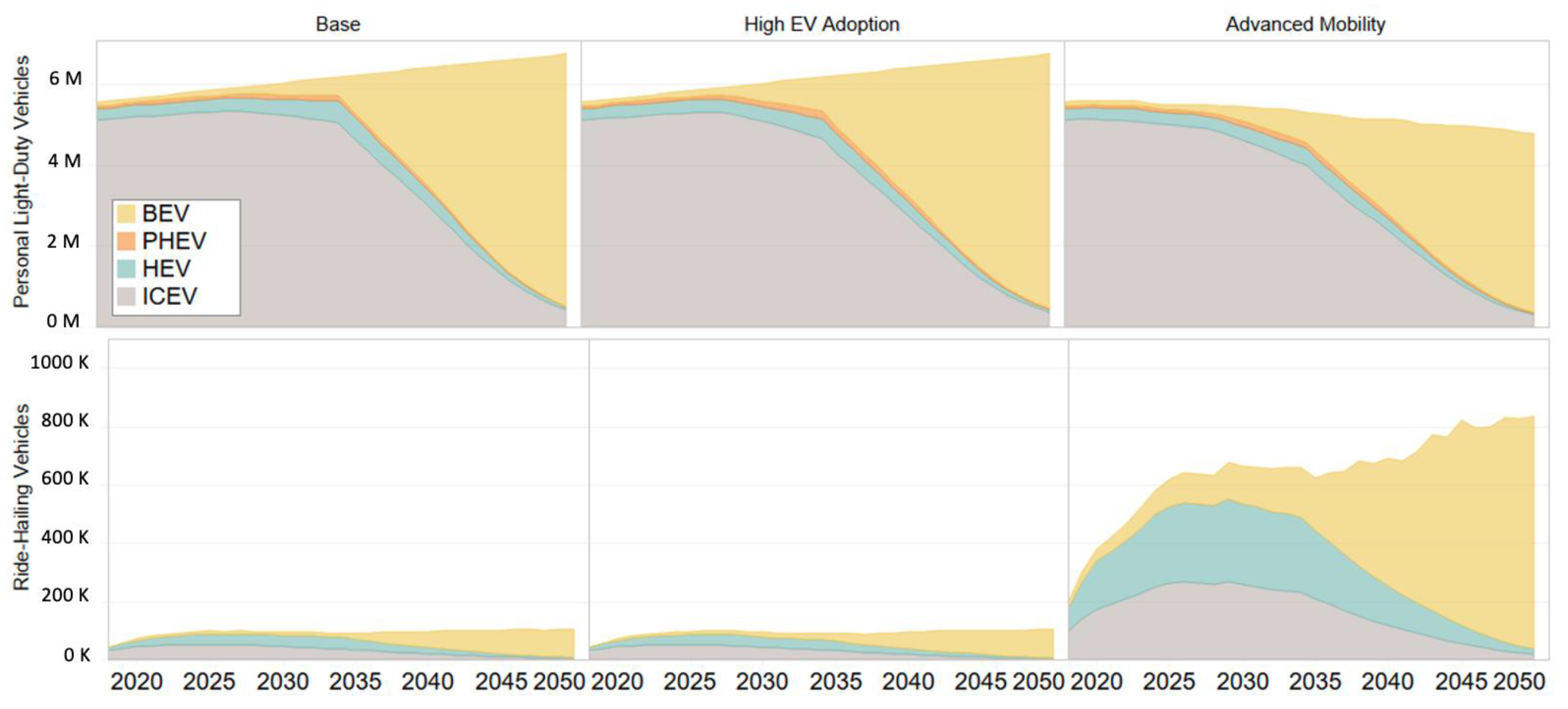
2.5. Transportation Scenarios

Transportation Energy and Mobility Pathway Options (TEMPO) is a comprehensive transportation demand macro model that can be used to explore long-term scenarios of energy use across all transportation segments and integrated with large multi-sectoral studies [32]. The inputs to TEMPO are developed at the county level, and they capture household income, initial vehicle stock, light-duty vehicle ownership, and vehicle class distribution data. The resulting output, which is in the form of a comma-separated values file of vehicle types, is read directly by BEAM to assign vehicle types according to the corresponding probability distribution. Four scenarios are identified (Figure 3) through TEMPO to capture a range of possible future scenarios and impacts on the fast-charging operation. The base scenario is used for the initial results in this paper to demonstrate the viability of the co-simulation framework and separated into three different scenarios (scenarios 1–3). The other transportation scenarios will be applied in future work with a more in-depth analysis. The current corresponding assumptions for the scenarios include:

1.

Base (2035)

○

Vehicle cost and performance consistent with the U.S. Energy Information Administration’s Annual Energy Outlook 2018;

○

A sales ban on non-zero emission vehicles (non-ZEVs) starting in 2035 (consistent with the phasing out in California of non-ZEVs);

○

Technology deployment levels consistent with the 2035 fleet (less turnover of vehicle stock).

2.

Base—Scenario 1

○

All agents with EVs have access to a home charging;

○

Unlimited home, work, and public charging infrastructure;

○

Destination charging only;

○

No co-simulation of the transportation and grid models.

3.

Base—Scenario 2

○

All agents with EVs have access to home charging;

○

Constrained home, work, and public charging infrastructure;

○

Destination charging only;

○

Co-simulation of the transportation and grid models.

4.

Base—Scenario 3

○

Approximately 87% of agents with EVs have access to home charging;

○

Constrained home, work, and public charging infrastructure;

○

En route and destination charging;

○

Co-simulation of the transportation and grid models.

5.

High EV Adoption (2040)

○

Vehicle cost and performance improvements for PEVs based on the National Renewable Energy Laboratory’s (NREL’s) Annual Technology Baseline’s 2020 Advanced scenarios;

○

Non-ZEV sales ban starting in 2035;

○

Technology deployment levels consistent with the 2040 fleet (i.e., higher turnover of vehicle stock).

6.

Advanced Mobility (2040)

○

Advanced ride-hailing: 50% reductions in cost and time;

○

Option for households to drop personally owned vehicles;

○

Automation assumed for ride-hailing fleets (i.e., reduced cost).

7.

Max EV Adoption (2050)

○

Technology deployment levels consistent with the 2050 fleet—almost full turnover of vehicles after the non-ZEV ban.

2.6. EV Charging Infrastructure

Next, the charging stations are placed using parcel data, adoption statistics, and transportation charging demand data to assure that chargers are placed in a realistic manner for the number of vehicles on the road. To do so, BEAM is first run with unlimited charging infrastructure, meaning it is assumed that vehicles can charge anywhere they can park. To avoid situations where most people are charging with public chargers or work chargers, a range constraint is imposed on vehicles when they charge in public, and the resulting charging behavior is validated against the EVI-Pro Lite output, using equivalent scenario assumptions [33]. This unlimited charging scenario gives insight into where vehicle operators would like to charge if they had the opportunity, with a slight preference to charge when at home for personally owned vehicles. If a charging event occurs at a home, a unique home identifier is provided to differentiate home chargers and prevent neighbors from using each other’s home chargers. At this stage, BEAM reports charging loads at each timestep for each TAZ along with the charging station type. The TAZs are tessellated polygons that cover areas about the size of a few city blocks. When all TAZs are put together, they cover the entire modeled region. The charging station type is broken down into public or private and by charging level (level 1, level 2, DCFC).

The unconstrained charging information is then overlaid with the area’s land parcel data, such that a home charging event station be placed at a home within that TAZ. The used parcel data contain many types of land uses, including residential uses with subsets of single-family homes and multi-family housing; commercial uses with subsets of groceries, retail space, theaters, offices, and hotels; and industrial use. The residential land use data also provide information on which type of parking is available, including street, driveway, single-family garage, parking lot, and multi-family garage options.

Next, charging stations are placed in each TAZ at parcel locations that match the charging event requirements. If two charging events with the same event details occur at subsequent timesteps, then this does not necessitate a new charger. However, if two charging events with the same event details occur at the same timestep, then a new charger must be placed to accommodate the charging demand. For example, if there is one at-home charging event in the morning at housing ID 1 and another charging event in the evening at housing ID 1, then the home with housing ID 1 only needs 1 charger. However, if there are two charging events at housing ID 1 at 9 a.m., then that home requires two chargers. In some instances, there may be more events in a given TAZ than can be accommodated. For example, if the charging is unrestricted then many vehicles may charge in the same TAZ at a residential charging station, but there may not be enough parking spots that would have access to charging. In cases like this, the maximum number of chargers of that type are placed at parcels within that TAZ, and any unmet charging demand is redirected to other charger types or other TAZs.

Once charging stations are assigned to parcels, and thereby TAZs, BEAM is run again with the charging restricted to charging only at the stations that were placed. If this new BEAM simulation shows sufficient ability to meet the charging demand, the stations can be connected to the distribution system model for co-simulation. The parcel locations and charging station types are used to create new lines, load points, and transformers if needed for the charging stations. Charging stations at residential, commercial, and industrial parcels where customer load points already exist still get new lines and load points to allow the charging load to be differentiated from other utility customer loads.

Finally, with the charging stations connected, BEAM and PyDSS can be run in a co-simulation via HELICS, such that charging loads are added to the distribution model at each timestep.

3. Results and Discussion

This section demonstrates the feasibility of the co-simulation architecture for capturing high-resolution transportation events and the impacts on the distribution grid down to the individual utility customer level through the initial analysis of a few representative scenarios. The preliminary results show that impacted distribution buses are concentrated near the urban centers and occur primarily when EVs charge at home before leaving for work or during the morning rush hour on their way to work. The geographic concentration of grid impacts implies that grid upgrades could be focused on certain areas to allow this level of EV adoption. The temporal concentration implies that the use of load shifting could be effective to integrate this level of EV charging on the grid. A few short-duration, very high-power demand periods are also seen from larger public chargers. This suggests that the use of charging station management strategies or on-site storage facilities could provide significant grid benefits. The interactions among grid upgrades, site power management strategies, and smart charging controls will be explored in later studies, which will build on this framework.

3.1. Simulation Scenarios

This co-simulation framework was used to explore three proof-of-concept scenarios:

• Base (2035)—Scenario 1: No EV charging;
• Base (2035)—Scenario 2: Base EV charging;
• Base (2035)—Scenario 3: Base EV charging with increased en route charging.

Scenario 1 provides a basis for comparison for grid conditions without EVs. Scenario 2 and scenario 3 enable the grid impacts to be compared with different charging patterns. In general, en route charging favors the use of higher charge rate public chargers, including those allowing extreme fast charging (XFC). Interestingly, the load profiles do not show much difference during home charging, in part because of the inclusion of travel events outside the study area. However, we can still observe a drop in the overall total energy charged in scenario 3 due to a drop in the number of home charging events, as drivers chose to charge en route more often. These impacts and the corresponding increase in XFC as an alternative solution to charging at home can be seen in Figure 4.

Each of these scenarios is studied for the Oakland–Alameda area, including industrial, urban, and suburban areas, along with many types of commercial and residential parcels. This diversity lends itself to testing before scaling up to the full San Francisco Bay Area. For the deployment of DER, all scenarios use the medium DER adoption case from SMART-DS. Specifically, the SMART-DS SFO v1.0 dataset subregion labeled P13U is used with medium solar placement and low battery placement as defined in the SMART-DS database.

Five-minute co-simulation timesteps are selected so results are of fine enough resolution that most charging sessions occur over more than one timestep but coarse enough that estimated steady-state load profiles and real data for solar profiles can be used without interpolation. The BEAM simulation is run with a finer second-by-second resolution to capture the plug-in and un-plug events that are between timesteps, but the charging loads are published to the distribution system in 5-min intervals.

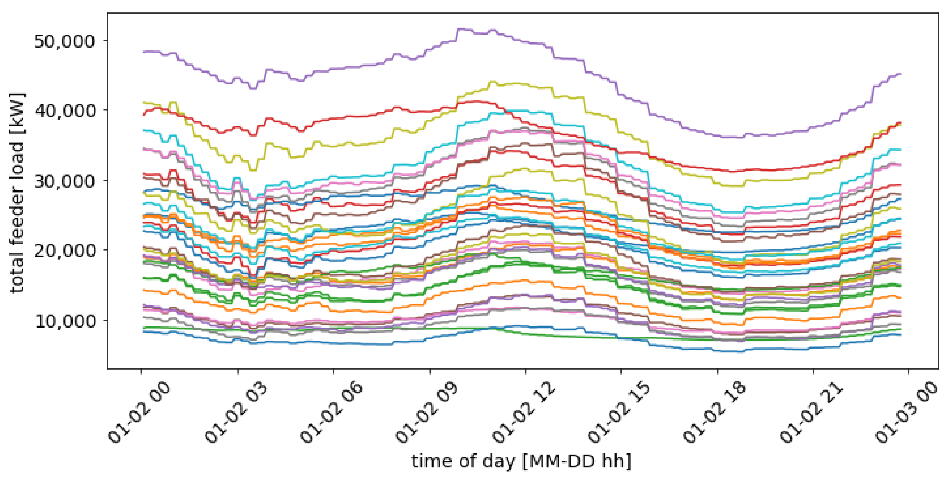
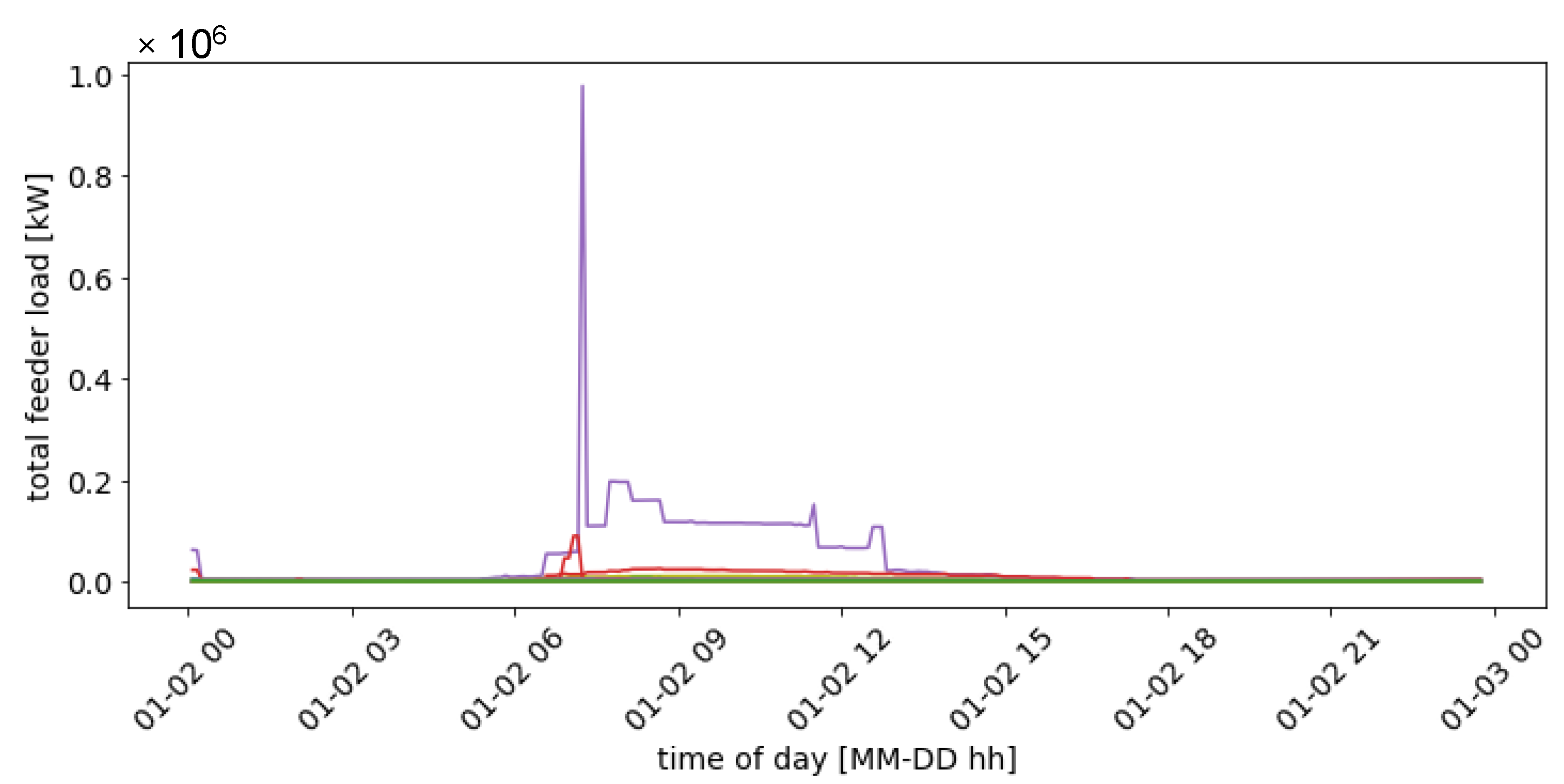
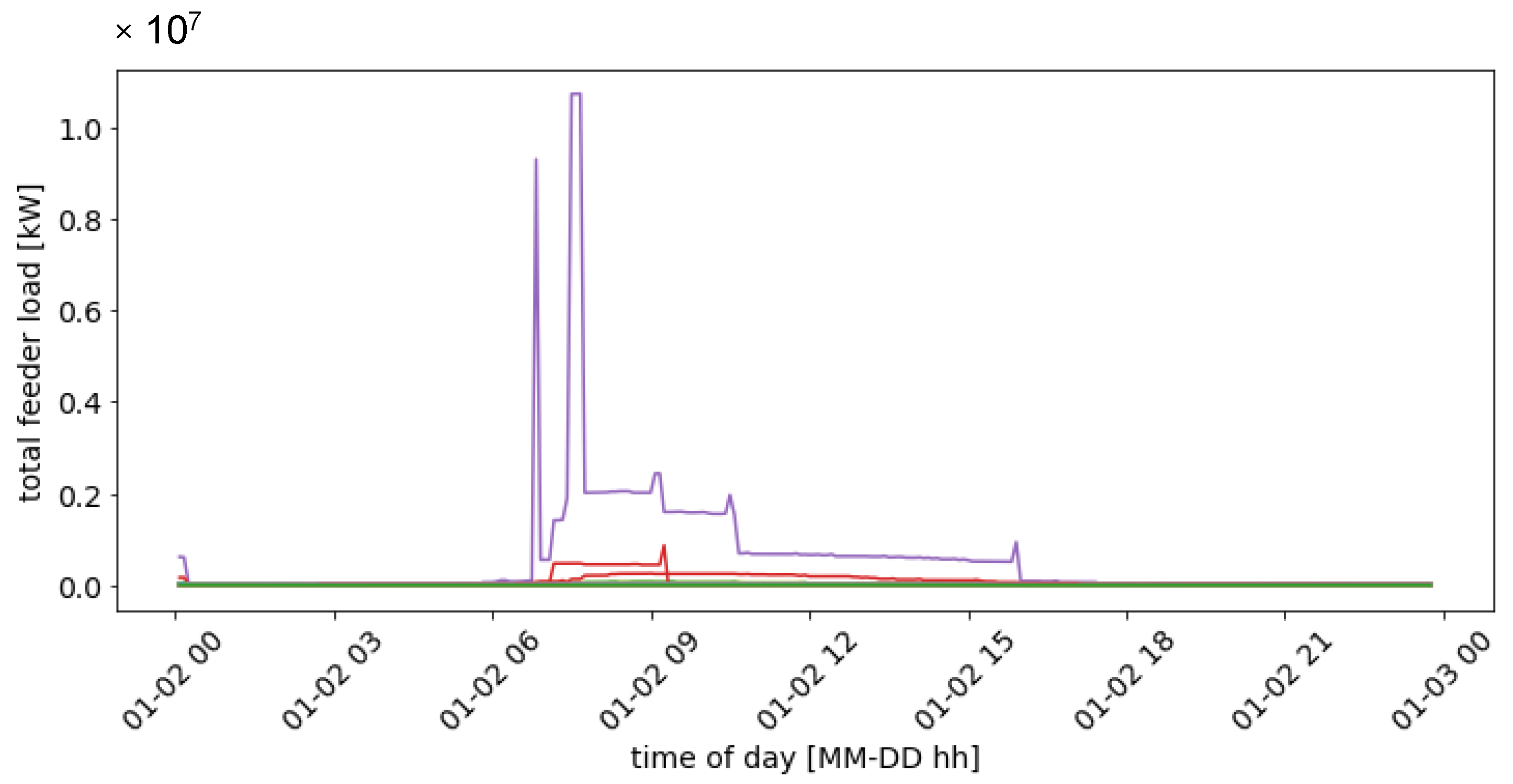
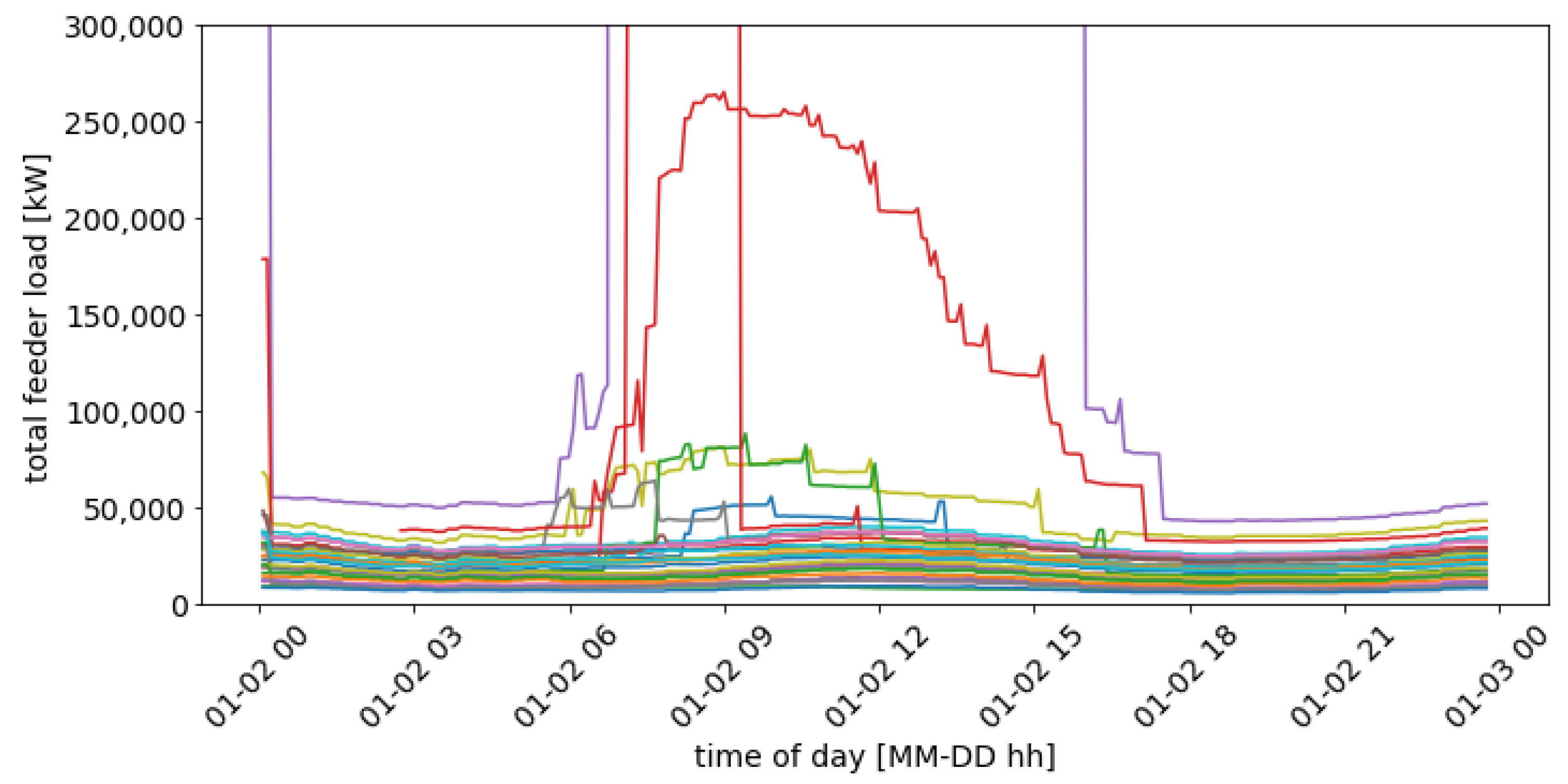
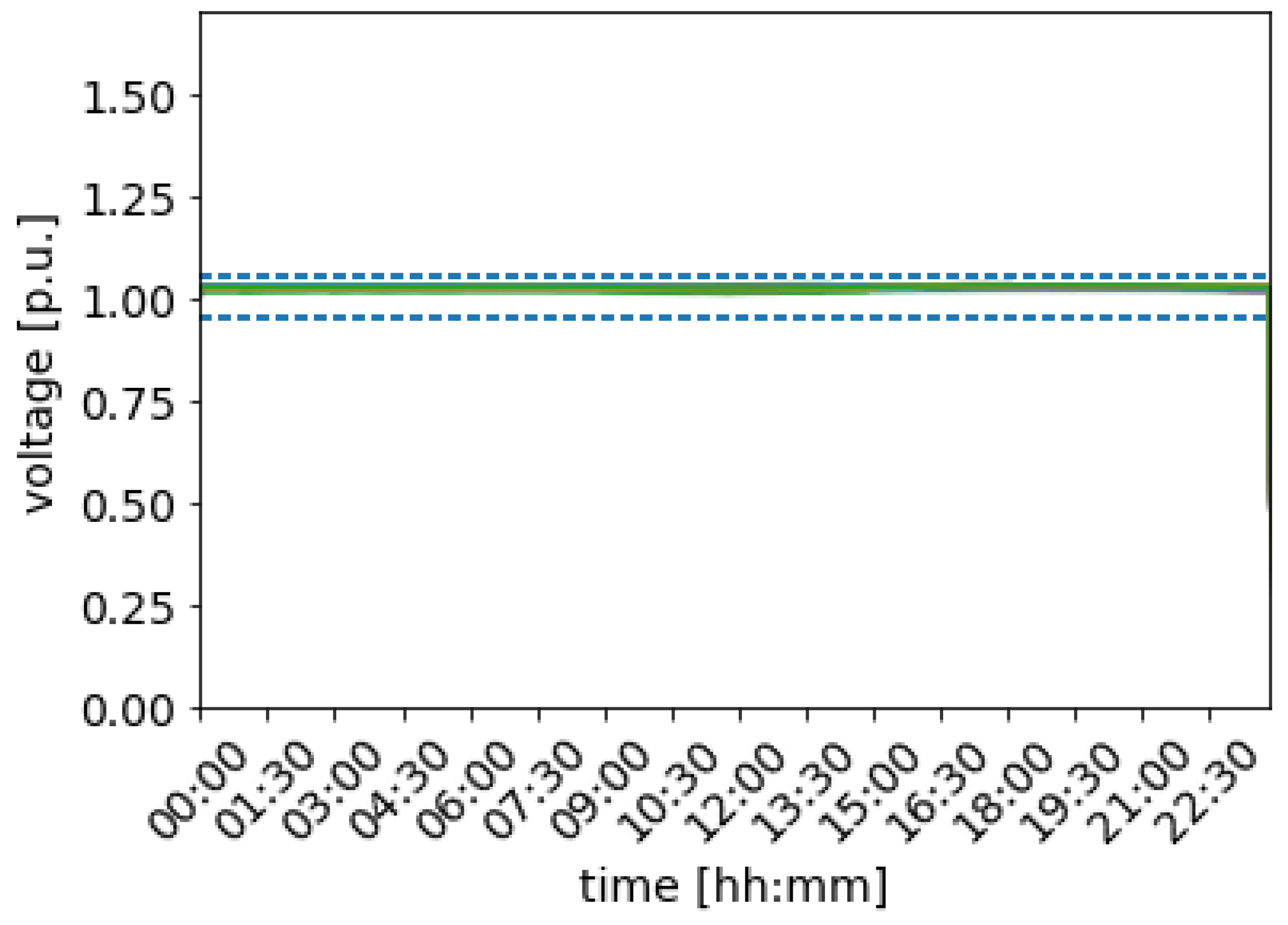
3.2. Charging Loads and Grid Impacts

The non-EV load shapes from scenario 1 (Figure 5) represent a midday peak load without EV charging for nearly all feeders, as simulated on January 2. Electrical loads in this winter season tend to peak at midday, whereas in summer months there can be a dual peak pattern, where the fan and air conditioning loads often cause elevated electrical loads in the evening hours as well as at midday.

The total EV charging loads are simulated in BEAM for at least 36 h to capture late night and early morning charging behaviors and charging loads from midnight through 5 a.m. on the second day replace the first 5 h of the load to maintain a 24-h simulation, as seen in Figure 6. The simulated twenty four hours of charging are used in the co-simulation with the distribution system to create a full day co-simulation. These loads are the total loads as published from BEAM in the HELICS co-simulation, and the charging loads inside the Oakland–Alameda region are read and recorded by the PyDSS federates as additional loads on the distribution system.

Many charging events that occur outside the Oakland–Alameda region are simulated for this initial proof of concept. These outside charging events occur from vehicles that move through the area and are tracked in the simulation but that charge in other locations. The EV charging loads in these future scenarios with high adoption rates of EVs and unmanaged charging are higher than the total grid loads without charging. When the total grid loads with EV charging in Figure 5 and Figure 7 are compared with EV charging loads within the Oakland–Alameda areas in Figure 4, the peaks for feeder loads can be seen to align with the peak charging hours, verifying that charging loads are passed correctly from BEAM through the HELICS interface to the distribution system model.

The charging loads as transmitted to the distribution system through HELICS have a tapered shape into the next day and exclude morning charging before 4:30 a.m., indicating that at least two days should be simulated so that early morning and late evening loads can be accurately represented without influence from the boundary conditions at midnight. Future studies will include this adjustment to incorporate early morning and late evening loads correctly.

The total feeder loads without EV loads shown in Figure 5 can be compared with the total load after adding charging, as shown in Figure 7. The drastic increase in load is especially apparent when the y-axis scale is noted. The sharp spikes in the distribution system load coincide with the first charging events of the day in the Oakland–Alameda area when the grid voltage drops, as many EVs plug in simultaneously and XFC events begin. The zoomed-in loads plotted in Figure 8 show that for many feeders, the EV charging has little impact on the total load profile, but for a few feeders the impact is stark, implying that the charging is concentrated in a few areas and that distribution upgrades could be focused on those areas.

The en route charging in scenario 3 increases the number of extremely high charge spikes, but otherwise causes loads to be distributed across more feeders and to occur at different times throughout the day. The total feeder loads for scenario 3 are shown in Figure 9, with a zoomed-in display of the total loads shown in Figure 10. Enabling en route charging creates additional peaks in the morning and additional XFC events when vehicles charge on the way to work. It also spreads some loads to later periods, when vehicles can stop to charge on the way to destinations and when doing so alleviates some of the midday loading on the heaviest loaded feeders. Similar to scenario 2, many feeder loads are not significantly impacted by the charging loads, showing that while increasing the diversity in available styles impacts more feeders, the main impacts are concentrated on a few feeders, indicating that distribution system upgrades could be focused on a few areas.

These proof-of-concept scenarios are used to analyze the distribution bus voltage impacts and suggest that future analyses should include impact mitigation strategies. For scenario 1 without EV charging, the voltages can be maintained within ANSI range A simply by adding volt–var control at all PV inverters. When distributed storage control is added to optimize for self-consumption for consumer-owned storage and for peak shaving for utility owned storage, the voltages are leveled out further, with very few buses outside ANSI range A over the course of a full day. Figure 11 shows the mean bus voltages by substation feeder group (multiple feeders per feeder group). Each line shows the average voltage for all nodes on a given feeder group and the 95% range of all nodes on that feeder group as a shaded region around the line. For scenario 1, all voltages are tightly aligned given the use of PV installations and storage inverters for voltage regulation and the lack of additional EV loads. The voltages in the 95% envelope of voltages are all very close to the mean. Before the EV loads are added, the voltages are generally on the high side of the acceptable range.

When EV loads are added, many buses dip below ANSI range A, and those that stay within the range are generally on the lower side of the acceptable range compared to without charging, as seen in Figure 12. Again the 95% envelopes are very close to the mean voltages for each feeder group, but they are non-zero, making the lines appear fuzzy. PyDSS simulates voltage collapse at buses on the feeder, represented in red in early morning. This zero-voltage indicates that this feeder group cannot support the addition of so many charging stations or the large loads from EV charging, especially when vehicles connect in early morning, before PV generation installations comes online. The feeder groups validate the hypothesis that grid upgrades or managed charging strategies are required to support a 15% adoption rate of electric passenger vehicles and the corresponding morning charging peak loads. The distribution grid in congested areas will experience the most impacts on voltages, especially given the short morning window of charging, which shifts the peak load times relative to having no EVs on the system. Other feeder groups and associated feeders experience voltage drops in alignment with the charging loads, but only three feeder groups out of 32 remain below ANSI range A for a large portion of the day; a few more feeder group averages dip below 0.95 p.u. infrequently. Most dips in voltage align with feeder increases in loads and are not the result of additional charging interconnections without loads.

When en route charging is added in scenario 3, the voltages drop slightly more on the impacted buses and for all buses except for those on the feeders represented by the red line, as seen in Figure 13. This is caused by an increased dispersal of vehicle charging events in scenario 3, alleviating some of the morning loads from the feeders represented in red, but increasing loads on several other feeders.

3.3. Spatial Analysis

When examining EV charging impacts and potential integration solutions, a spatial analysis is important, especially when evaluating whether smart charging can favor charge events during periods of lower feeder loading. Visualizations of the distribution voltage were developed and are compared side by side with graphical representations of EV charging events in Figure 14. Given the adoption of solar and storage instillations, the distribution system has a voltage that is slightly high but within ANSI range A for most buses at most timesteps. When EV charging loads are added, most bus voltages drop, some dip below ANSI A range, and a few exhibit very low voltages outside ANSI range B. As shown in Figure 15, low-voltage excursions (orange dots), high-voltage excursions (pink dots), and zero voltages (black dots) are concentrated around the downtown areas of Oakland and Alameda, where most charging occurs. They appear prevalently in the 6 p.m. snapshot when the PV solar generation has decreased and travelers plug in vehicles after rush hour.

On the transportation side, we can observe more frequent and intense charging events occurring at noon and in early morning, when individual agents start traveling at 8 a.m., in this example region. The charging loads remain relatively high throughout the midday hours, dropping off in the evening and overnight hours.

The results of the distribution system simulation of all three charging scenarios are summarized in

Table 3. Distribution system impact results summary by charging scenario.

Scenario	Results Summary
Scenario 1: No EV charging	Minimal voltage excursions, no sharp load spikes
Scenario 2: Base EV charging	Voltage excursions especially in morning, load spikes during morning and midday
Scenario 3: Base EV charging with increased en route charging	Voltage excursions especially in morning and midday, load spikes during morning and midday, especially in urban centers

, showing that charging increases voltage excursions and component loadings, and increased en route charging increases impacts during midday and in urban centers.

3.4. Discussion and Future Work

The proof-of-concept results shown in this paper demonstrate that the co-simulation framework accurately shares high-fidelity model outputs between transportation and distribution systems at each timestep. These preliminary results represent a pessimistic view of what impacts the grid may incur if charging were unlimited and no distribution system hardware upgrades or charging controls were implemented as improvements from existing distribution systems. It is expected that with high future EV adoption rates, some controls or incentives to shift the charging location and time would be used, in addition to distribution system hardware upgrades and possibly DER coordination to improve the grid’s EV hosting capacity. These factors are likely to improve the grid performance, even with increasing electrification, and they will be explored in later work.

In future work, this analysis will be extended by exploring scenarios to cover the full San Francisco Bay Area for both the medium DER case shown here and a high DER case. The two grid scenarios will be analyzed with EV charging stations and loads from several transportation scenarios representing different EV adoption levels, autonomous vehicle prevalence rates, and ride-hail prevalence rates.

The full set of scenarios will first be evaluated, analyzed, and compared without any smart charging or charging controls in place. In the uncontrolled charging scenarios, grid upgrade assessments will be used to determine the kinds of changes and costs that would be needed to support uncontrolled charging. After those grid-based measures are determined, several charging control strategies will be tested and compared for their efficacy using metrics such as grid voltages, charging wait times, traveler costs, and reductions in upgrade costs.

4. Conclusions

This work describes the co-simulation used to connect vehicle-level transportation simulations for the Oakland–Alameda area with a distribution system simulation at the individual customer level in the steady state for the same area. The transportation software BEAM is run in the co-simulation with the gird simulation in PyDSS via the HELICS co-simulation framework to evaluate uncontrolled charging impacts on distribution systems. The preliminary results suggest that volt–var inverter controls at distributed PV and storage locations can maintain high-fidelity distribution grids for scenarios with some EV adoption, but further controls or upgrades are needed for increased adoption and in areas with higher concentrations of charging. The results also suggest that any over-voltages from distributed PV and storage instillations could be mitigated with inverter controls and moderate levels of EV charging. Future studies will more thoroughly analyze the transportation and grid scenarios with different control approaches to evaluate the best types of controls and upgrades for each scenario.

References

1. Muratori, M.; Alexander, M.; Arent, D.; Bazilian, M.; Cazzola, P.; Dede, E.; Farrell, J.; Gearhart, C.; Greene, D.; Jenn, A.; et al. The Rise of Electric Vehicles—2020 Status and Future Expectation. Prog. Energy 2021, 3, 022002. Available online: https://0-iopscience-iop-org.brum.beds.ac.uk/article/10.1088/2516-1083/abe0ad/meta (accessed on 17 February 2023). [CrossRef]
2. Panossian, N.; Muratori, M.; Palmintier, B.; Meintz, A.; Lipman, T.; Moffat, K. Challenges and Opportunities of Integrating Electric Vehicles in Electricity Distribution Systems. Curr. Sustain. Energy Rep. 2022, 9, 27–40. [Google Scholar] [CrossRef]
3. U.S. DRIVE Grid Integration Technical Team (GITT); Integrated Systems Analysis Technical Team (ISATT). Summary Report on EVs at Scale and the U.S. Electric Power System 2019. Available online: https://www.energy.gov/eere/vehicles/downloads/summary-report-evs-scale-and-us-electric-power-system-2019 (accessed on 24 June 2021).
4. Venegas, F.G.; Petit, M.; Perez, Y. Active integration of electric vehicles into distribution grids: Barriers and frameworks for flexibility services. Renew. Sustain. Energy Rev. 2021, 145, 111060. [Google Scholar] [CrossRef]
5. Alame, D.; Azzouz, M.; Kar, N. Assessing and mitigating impacts of electric vehicle harmonic currents on distribution systems. Energies 2020, 13, 3257. [Google Scholar] [CrossRef]
6. Clement-Nyns, K.; Haesen, E.; Driesen, J. The Impact of Charging Plug-In Hybrid Electric Vehicles on a Residential Distribution Grid. IEEE Trans. Power Syst. 2010, 25, 371–380. [Google Scholar] [CrossRef] [Green Version]
7. Affonso, C.M.; Kezunovic, M. Technical and Economic Impact of PV-BESS Charging Station on Transformer Life: A Case Study. IEEE Trans. Smart Grid 2019, 10, 4683–4692. [Google Scholar] [CrossRef]
8. Fachrizal, R.; Ramadhani, U.H.; Munkhammar, J.; Widén, J. Combined PV–EV hosting capacity assessment for a residential LV distribution grid with smart EV charging and PV curtailment. Sustain. Energy Grids Netw. 2021, 26, 100445. [Google Scholar] [CrossRef]
9. Lopes, J.A.P.; Soares, F.J.; Almeida, P.M.R. Integration of Electric Vehicles in the Electric Power System. Proc. IEEE 2011, 99, 168–183. [Google Scholar] [CrossRef] [Green Version]
10. Shukla, A.; Verma, K.; Kumar, R. Multi-objective synergistic planning of EV fast-charging stations in the distribution system coupled with the transportation network. IET Gener. Transm. Distrib. 2019, 13, 3421–3432. [Google Scholar] [CrossRef]
11. Lin, H.; Bian, C.; Wang, Y.; Li, H.; Sun, Q.; Wallin, F. Optimal planning of intra-city public charging stations. Energy 2022, 238, 121948. [Google Scholar] [CrossRef]
12. Clairand, J.-M.; Gonzalo-Rodriguez, M.; Kumar, R.; Vyas, S.; Escriva-Escriva, G. Optimal siting and sizing of electric taxi charging stations considering transportation and power system requirements. Energy 2022, 256, 124572. [Google Scholar] [CrossRef]
13. Kong, W.; Luo, Y.; Feng, G.; Li, K.; Peng, H. Optimal location planning method of fast charging station for electric vehicles considering operators, drivers, vehicles, traffic flow and power grid. Energies 2019, 186, 116826. [Google Scholar] [CrossRef]
14. Palensky, P.; Widl, E.; Stifter, M.; Elsheikh, A. Modeling Intelligent Energy Systems: Co-Simulation Platform for Validating Flexible-Demand EV Charging Management. IEEE Trans. Smart Grid 2013, 4, 1939–1947. [Google Scholar] [CrossRef]
15. Zhang, H.; Sheppard, C.; Lipman, T.; Moura, S. Joint Fleet Sizing and Charging System Planning for Autonomous Electric Vehicles. IEEE Intell. Transp. Syst. Trans. 2019, 21, 4725–4738. [Google Scholar] [CrossRef] [Green Version]
16. Dong, X.; Mu, Y.; Xu, X.; Jia, H.; Wu, J.; Yu, X.; Qi, Y. A charging pricing strategy of electric vehicle fast charging stations for the voltage control of electricity distribution networks. Appl. Energy 2018, 225, 857–868. [Google Scholar] [CrossRef]
17. Leou, R.-C.; Su, C.-L.; Lu, C.-N. Stochastic Analyses of Electric Vehicle Charging Impacts on Distribution Network. IEEE Trans. Power Syst. 2014, 29, 1055–1063. [Google Scholar] [CrossRef]
18. Manbachi, M.; Sadu, A.; Farhangi, H.; Monti, A.; Palizban, A.; Ponci, F.; Arzanpour, S. Impact of EV penetration on Volt–VAR Optimization of distribution networks using real-time co-simulation monitoring platform. Appl. Energy 2016, 169, 28–39. [Google Scholar] [CrossRef]
19. Neaimeh, M.; Wardle, R.; Jenkins, A.M.; Yi, J.; Hill, G.; Lyons, P.F.; Hübner, Y.; Blythe, P.T.; Taylor, P.C. A probabilistic approach to combining smart meter and electric vehicle charging data to investigate distribution network impacts. Appl. Energy 2015, 157, 688–698. [Google Scholar] [CrossRef] [Green Version]
20. Taylor, J.; Maitra, A.; Alexander, M.; Brooks, D.; Duvall, M. Evaluations of plug-in electric vehicle distribution system impacts. In Proceedings of the IEEE PES General Meeting, Minneapolis, MN, USA, 25–29 July 2010; pp. 1–6. [Google Scholar] [CrossRef]
21. Putrus, G.A.; Suwanapingkarl, P.; Johnston, D.; Bentley, E.C.; Narayana, M. Impact of electric vehicles on power distribution networks. In Proceedings of the 2009 IEEE Vehicle Power and Propulsion Conference, Dearborn, MI, USA, 7–10 September 2009; pp. 827–831. [Google Scholar] [CrossRef]
22. Sharma, I.; Canizares, C.; Bhattacharya, K. Smart Charging of PEVs Penetrating Into Residential Distribution Systems. IEEE Trans. Smart Grid 2014, 5, 1196–1209. [Google Scholar] [CrossRef]
23. Munkhammar, J.; Widén, J.; Rydén, J. On a probability distribution model combining household power consumption, electric vehicle home-charging and photovoltaic power production. Appl. Energy 2015, 142, 135–143. [Google Scholar] [CrossRef]
24. Palmintier, B.; Elgindy, T.; Mateo, C.; Postigo, F.; Gómez, T.; de Cuadra, F.; Martinez, P.D. Experiences developing large-scale synthetic U.S.-style distribution test systems. Electr. Power Syst. Res. 2021, 190, 106665. [Google Scholar] [CrossRef]
25. Sheppard, C.; Waraich, R. BEAM—Beam 0.7.0 Documentation. 2019. Available online: https://beam.readthedocs.io/en/latest/index.html (accessed on 29 September 2020).
26. Latif, A. NREL/PyDSS. National Renewable Energy Laboratory. 2020. Available online: https://github.com/NREL/PyDSS (accessed on 16 November 2020).
27. Palmintier, B.; Krishnamurthy, D.; Top, P.; Smith, S.; Daily, J.; Fuller, J. Design of the HELICS High-Performance Transmission-Distribution-Communication-Market Co-Simulation Framework. In Proceedings of the 2017 Workshop on Modeling and Simulation of Cyber-Physical Energy Systems, Pittsburgh, PA, USA, 21 April 2017. [Google Scholar] [CrossRef]
28. Krishnamurthy, D. OpenDSSDirect.py: Python Direct-Mode Interface to OpenDSS. 2020. Available online: https://github.com/dss-extensions/OpenDSSDirect.py (accessed on 16 November 2020).
29. OpenDSS. SourceForge. Available online: https://sourceforge.net/projects/electricdss/ (accessed on 16 November 2020).
30. Krishnan, V.; Bugbee, B.; Elgindy, T.; Mateo, C.; Duenas, P.; Postigo, F.; Lacroix, J.-S.; Roman, T.G.S.; Palmintier, B. Validation of Synthetic U.S. Electric Power Distribution System Data Sets. IEEE Trans. Smart Grid 2020, 11, 4477–4489. [Google Scholar] [CrossRef]
31. SMART-DS SFO 2018 OpenDSS Models. Available online: https://data.openei.org/submissions/2981 (accessed on 17 February 2023).
32. Muratori, M.; Jadun, P.; Bush, B.; Bielen, D.; Vimmerstedt, L.; Gonder, J.; Gearhart, C.; Arent, D. Future integrated mobility-energy systems: A modeling perspective. Renew. Sustain. Energy Rev. 2020, 119, 109541. [Google Scholar] [CrossRef]
33. Wood, E. Alternative Fuels Data Center: Electric Vehicle Infrastructure Projection Tool (EVI-Pro) Lite. Available online: https://afdc.energy.gov/evi-pro-lite (accessed on 2 November 2022).
Figure 1. Block diagram of co-simulation framework without smart charging.
Energies 16 02189 g001
Figure 2. The co-simulation block diagram of the transportation model BEAM configured for this work.
Energies 16 02189 g002
Figure 3. Light-duty vehicle fleet evolution in the San Francisco Bay Area.
Energies 16 02189 g003
Figure 4. The charger type balances and ratios of extreme fast charging use for scenario 2 and scenario 3.
Energies 16 02189 g004
Figure 5. Total feeder loads for scenario 1 without EV charging.
Energies 16 02189 g005
Figure 6. EV charging loads for scenario 2 and scenario 3.
Energies 16 02189 g006
Figure 7. Scenario 2 feeder loads with EV charging.
Energies 16 02189 g007
Figure 8. Scenario 2 feeder loads with EV charging rates zoomed-in to highlight lower load ranges.
Energies 16 02189 g008
Figure 9. Scenario 3 feeder loads with EV charging.
Energies 16 02189 g009
Figure 10. Scenario 3 feeder loads with EV charging zoomed-in to highlight lower load ranges.
Energies 16 02189 g010
Figure 11. Scenario 1 distribution feeder nodal voltage means and 95% range for all nodes plotted by substation feeder group.
Energies 16 02189 g011
Figure 12. Scenario 2 distribution feeder nodal voltage mean and 95% range for all nodes, plotted by substation feeder group.
Energies 16 02189 g012
Figure 13. Scenario 3 distribution feeder nodal voltage mean and 95% range for all nodes, plotted by substation feeder group.
Energies 16 02189 g013
Figure 14. Scenario 3 charging loads for select times of day.
Energies 16 02189 g014
Figure 15. Scenario 3 distribution system voltages for select times of day, with voltage excursions highlighted with orange and pink dots.
Energies 16 02189 g015