

A Tensile Rotary Airborne Wind Energy System—Modelling, Analysis and Improved Design

1
Wind Energy and Control Centre, Department of Electronic and Electrical Engineering, University of Strathclyde, 204 George Street, Glasgow G1 1XW, UK
2
Windswept and Interesting Limited, Nesbister, Shetland ZE2 9LJ, UK
*
Author to whom correspondence should be addressed.
†
Current address: REOptimize Systems, Edinburgh EH9 3BF, Scotland, UK.
Energies 2023, 16(6), 2610; https://0-doi-org.brum.beds.ac.uk/10.3390/en16062610
Submission received: 17 November 2022
/
Revised: 28 February 2023
/
Accepted: 6 March 2023
/
Published: 9 March 2023
(This article belongs to the Special Issue Airborne Wind Energy Systems)
Abstract
:A unique rotary kite turbine designed with tensile rotary power transmission (TRPT) is introduced in this work. Power extraction, power transmission and the ground station are modelled in a modular framework. The TRPT system is the key component of power transmission, for which three models with different levels of complexity are proposed. The first representation is based on the stationary state of the system, in which the external and internal torques of a TRPT section are in equilibrium, referred to as the steady-state TRPT model. The second representation is a simplified spring-disc model for dynamic TRPT, and the third one is a multi-spring model with higher degrees of freedom and more flexibility in describing TRPT dynamics. To assess the torque loss on TRPT, a simple tether drag model is written for the steady-state TRPT, followed by an improved tether drag model for the dynamic TRPT. This modular framework allows for multiple versions of the rotor, tether aerodynamics and TRPT representations. The developed models are validated by laboratory and field-testing experimental data, simulated over a range of modelling options. Model-based analysis are performed on TRPT design, rotor design and tether drag to understand any limitations and crucial design drivers. Improved designs are explored through multi-parameter optimisation based on steady-state analysis.
1. Introduction
Airborne wind energy (AWE) systems provide a unique form of power generation, in which tethered airborne devices are utilised to harness energy from the wind. With the use of lightweight components, AWE systems are able to access remote locations and higher altitudes, which may not be feasible for standard horizontal-axis wind turbines. A rotary kite AWE system has multiple wings connected together by tethers to form rotors. During the operation, the kite system is inclined to the incoming wind, and both the lift and the torque are generated using auto-rotation without any external torque applied [1].
1.1. A Brief History of Daisy-Kite AWE Rotary Kite Turbine
The Daisy Kite systems, developed since 2012 by Windswept and Interesting Ltd. (W&I), Shetland, UK [2], and their tensile rotary power transmission (TRPT) design were introduced in [3] and further analysed in [4]. TRPT enables a continuous power output with a ground-based generator. With this design, the rotors are made of multiple short blades tied together in a ring pattern. When flown, the rotor acts like a kite autogyro. The kite-turbine rotor blades sweep a relatively large annular band area as compared to standard rotors of the same blade length.
Early ring−kite rotors had simple constructions. The first prototype was a set of 4 × 2−line parafoil trainer kites, tied to an inflatable trampoline. This kite rotor was suspended by bridles fore and aft. The bridle ends were then gathered and tied to bearings set to two masts, one upwind and one downwind. The rotor was held in the air, its axis pointing into wind, the parafoil kites were unfurled to fill in the wind. When the rotor was released, it spun. The kite rotor would eventually stop spinning when the bearings could not keep up, and the bridles wound together, crushing the rotor. Field tests have now demonstrated that torque from a kite rotor is transmissible along bridles, and also revealed the inherent weakness of TRPT—that long axial bridles, close together and used for torque transmission, are prone to over-twisting.
Kite turbines are stretched out on the ground before launch. The lower ends of the TRPT lines are connected to the power take-off wheel on the ground station generator. Next, the top bearing of the turbine is connected to the line of a lifting kite. The lifting kite is launched and the turbine is released up into the air using the lower end of the lifting line (the backline). The kite turbine now acts as an autogyro in the wind. The spinning tethers transmit power to the generator. Figure 1 illustrates a typical configuration of a Daisy kite turbine.
Windswept and Interesting have implemented and assessed designs with various parameters, including the number of blades per rotor, blade geometries and bridle configurations, ring geometries, material selections, and fairings, etc. Variations of ring-kite turbine designs in tests have improved the system performance. Rings made from modular carbon-fibre tube sections are lighter and more rigid. Further rings of a smaller diameter were added to extend the length of lines which could reliably transmit torque. Faster rigid blades are used and proved to be more efficient; they require fewer bridles, which reduces line drag.
Multiple blade AWE systems increase AWE power-to-weight ratios by increasing total blade area without a significant mass penalty while also reducing tether drag [5]. In Daisy Kite’s operation, the turbine lines and rotor ring components work in tension as an inflated network. Extending this network patterning allows the deployment of multiple lightweight kite blades using minimal material mass. The kite turbines tests demonstrated airborne power-to-weight ratios are larger than 0.8 kW/kg. This particularly high power-to-weight ratio on a network-scalable system design may evolve to produce low-cost, clean energy if it can be flown at scale.
The rotors have a demonstrated ability for working in stacks. Several multi-stage kite turbines comprised of up to three layers have been tested. These taller kite turbines are more challenging to launch but exhibit smoother operation and have less line drag per blade area.
1.2. Motivation and Main Work Organisation
As a unique design in the AWE family, rotary kite systems have advantages in several aspects. (i) Rotary kite systems are designed to produce continuous power generation, which is different from other AWEs with cyclic power output. (ii) The design of networked wings reduces the control requirements for each wing and for the whole system. (iii) The networked wings provide a level of redundancy to the system, making safer turbine operation and increased robustness to environmental uncertainties. (iv) With the configuration of networked wings, the tether drag is reduced and the overall efficiency of the system is improved [6]. The benefits in (ii) and (iii) make rotary systems inherently more stable compared to AWE devices with lift and drag operation modes.
There have been several designs in the rotary kite family [7,8,9,10,11,12,13,14,15,16]; most of them are ground generation devices. In addition to the Daisy Kite introduced in Section 1.1, two other rotary AWE system designs also utilise TRPT. One is the configuration developed in [10] without intermediate rings between the ground station and the flying rings. Another configuration was developed to have the open tensegrity shaft that uses straight carbonfibre rods to separate eight tethers [13].
Rotary kite turbines present some advantages over the leading lift-and-drag AWE designs; many of these are qualitative based on observations from prototype testing. There is a lack of a systematic approach for modelling, simulation, analysis, control and performance assessment of rotary kite AWE systems (AWES). For the Daisy Kite AWES with TRPT, several small-scale AWE prototypes have been manufactured and tested; however, the design and operating characteristics of the TRPT systems are relatively unexplored in the academic literature. In this work, the main aim is to build a modular modelling framework for the Daisy Kite rotary AWES, giving mathematical representations to key components with a focus on TRPT modelling. The model will be validated by experimental data and numerical analysis. The developed model will be used for system analysis and optimisation design.
The remainder of this paper is organised as follows. The model development of the rotary kite turbine system is presented in Section 2 covering the subsystem models for power extraction and power take off. The core models on TRPT and tether aerodynamics are given in Section 3. Three presentations are proposed for TRPT, i.e., the steady-state model, the spring-disc dynamic model and the multi-spring dynamic model. In addition, two tether drag models are established using different assumptions. In Section 4, the developed models are tested and validated using collected experimental data, and several modifications are applied to improve the spring-disc and multi-spring TRPT models. Based on the developed models, comprehensive system analysis are performed on TRPT design, rotor design and tether drag design in Section 5. Furthermore, optimised designs are implemented based on the steady-state performance under assumed site conditions to maximise the power output of the rotary kite system. Conclusions are given in Section 6. Pseudo codes of model developments for the spring-disc and multi-spring TRPT dynamic models are given in Appendix A. The configurations of the several TRPTs used in this work are given in Appendix B. Some more testing results of the multi-spring TRPT model are shown in Appendix C.
2. Modelling Framework
The purpose of modelling is to develop dynamic representations of the rotary ring kite AWES that utilises TRPT for torque transmission. It’s a first attempt to establish such a model with the supporting data from the Daisy Kite system, developed by W&I. To start with, the general modelling aspects are introduced in this section, more specific modelling on TRPT and tether aerodynamics will be presented in Section 3.
2.1. Overall System Configuration
The full system model consists of a series of connected individual modules which can be grouped into function blocks of power extraction, power transmission and ground station. A block diagram of the modelling framework is shown in Figure 2, including modules and their connections within the rotary AWES model. Power-extraction modelling is presented in Section 2.2 covering rotor aerodynamics, wing characteristics, lift kite aerodynamics and wind models used in this work. The power take off is summarised in Section 2.3. Modelling of TRPT for power transmission is given in Section 3, in which the steady-state model is developed to capture the global static behaviour of the TRPT system, the dynamic models are established to characterise the dynamics of TRPT, and two tether drag models are proposed to calculate the torque loss within TRPT.
2.2. Power Extraction
2.2.1. Rotor Aerodynamics
The rotary kite AWES uses multiple wings to form rotors; the wings are connected to each other at a distance from the centre of rotation, making an open centre around the hub. An elevation angle is required for rotary AWES, and the rotor is tilted/pitched down into the incoming flow. This causes a misalignment between the rotor plane and the wind vector, analogous to a yawed-horizontal axis wind turbine (HAWT). Two modelling methods, the actuator disc model and blade element momentum (BEM) theory, were used for the rotary AWES representation.
The actuator disc model provides an initial estimate of power output achieved at a given rotor geometry, in certain wind speeds and at a given elevation angle. The power output from a rotor is calculated by
where is the air density, the wind speed, A the swept area of the rotor, the power coefficient and the elevation angle.
With BEM, the lift and drag coefficients are assumed to vary with the angle of attack based on steady flow values. Rotary AWES rotors are constantly yawed due to the necessary elevation angle applied. Yawed rotors may experience unsteady aerodynamic effects which results in the blades experiencing dynamic stall. Therefore, the use of steady-state 2D lift and drag coefficients in BEM for the modelling of rotary AWES rotors needs to be further examined. The studies in [17,18,19,20] demonstrate that for yaw angles of up to 45°, the results from BEM are comparable to experimental data, but that BEM becomes less accurate as the yaw angle becomes larger. They also show that BEM is less accurate at the blade tip and root, for high wind speeds and for higher tip speed ratios. Given this evidence, the use of BEM to represent the rotor aerodynamics of rotary AWES is considered to be suitable for low elevation angles up to 30°, wind speeds up to 14 m/s, and for tip speed ratios of less than 7. In this work, AeroDyn v15 was used as the Rotor Aerodynamics module within the rotary AWES model. See [4] for more details.
2.2.2. Wing Characteristics
A key input into the Rotor Aerodynamics module are the aerodynamic properties of the wings used within the rotor. AeroDyn requires the lift and drag coefficients of each wing, for all possible angles of attack, from 0° to 360°. Two types of wings are used by various Daisy Kite prototypes, the HQ Symphony Beach III 1.3 kite and the bespoke foam blades using the NACA 4412 aerofoil profile.
The HQ Symphony Beach III 1.3 kite is widely available. The wings’ performance coefficients are estimated from the available literature. The HQ kite is a ram-air kite with a span of 1.3 m and a chord which varies from 0.55 m at the centre to 0.16 m at the tips. To identify relevant aerodynamic characteristics, the Reynolds number () and aspect ratio () of the wing were calculated. The wind-tunnel test results shared in [21] were used to predict the lift and drag coefficients of the HQ Symphony Beach III 1.3 kite for angles of attack from 0° to 30° in this work. Outside of this range, the coefficients were calculated using NREL’s AirfoilPrep [22].
Given the wide and extensive use of NACA aerofoil profiles, the aerodynamic performance coefficients for the NACA 4412 foam blades were defined based on wind-tunnel test data from the available literature and Xfoil. Provided with the 2D shape of an aerofoil, Xfoil calculates the lift and drag coefficients for a given and Mach number. The foam blades have a span of 1 m and a constant chord length of 0.2 m. The for the foam blades is calculated to be 1.4 × 10⁵ and to be 5. The results presented in [23], along with the predictions from Xfoil [24], were used to define the lift and drag coefficients for the foam blades for angles of attack in the range from −10° to 110°. For values outside of this range, similar to the HQ kites, the coefficients were calculated using NREL’s AirfoilPrep.
2.2.3. Lift-Kite Aerodynamics
The lift kite is represented as a static point force. Using the lift-kite area, S; the lift coefficient, ; and the drag coefficient, , the calculations of lift-kite aerodynamic forces are given in (2). The values taken were: , and Assuming the elevation angle of the lift-kite tether is equal to the elevation angle, , of the TRPT and rotor, the lift kite’s aerodynamic force, which is in-line with the lift-kite tether , can be calculated by
2.2.4. Wind Models
Three wind models were used for modelling and simulation in this work.
- (1)
- The first is the uniform and constant wind speed used to analyse steady-state performance.
- (2)
- The second wind model assumes that the wind speed varies with time but is uniform in the plane perpendicular to the wind’s direction. This model is used for the simulation of dynamic system responses.
- (3)
- The third wind shear model accounts for the variations in wind speed in both time and altitude. The variation in wind speed with altitude is calculated following the power law [25]. This wind shear model is used for the entire system to integrate all modules into the same modelling scheme.
2.3. Ground Station—Power Take Off
The ground station consists of several components and houses the system’s drivetrain. The driventrain components include, a wheel, which the TRPT connects to; a chain drive; a power meter; a disc brake and the generator. To account for the rotating mass of the drivetrain, the mass of the bottom TRPT ring was made to be heavier than the upper rings in the TRPT. The bottom ring of the TRPT represents the wheel on the ground station to which the TRPT is connected. This wheel is made from stainless steel and has a larger mass compared to the other rings of the TRPT constructed from carbon-fibre tubes. This wheel (0.85 kg, outer radius 0.21 m) and the generator (5.5 kg, radius 0.12 m) account for most of the rotating mass within the ground station. The moments of inertia of the generator and wheel are calculated to be 0.040 kgm2 and 0.019 kgm2, respectively. Other moments of inertia grouping the inertia due to the chain drive, disc brake and power meter, were calculated to be 0.002 kgm2 in this work.
The load from the generator is represented as a resisting torque applied to the lowest ring of the TRPT. For initial simulations, this was kept at a constant value before step changes were applied to analyse the TRPT and rotor responses. The torque measured at the bottom of the TRPT during experimental tests was also used to set the generator torque within simulations, which allows a more direct comparison between the model and the field tests.
3. Power Transmission—TRPT Representations and Tether Drag Models
In this section, the developed models corresponding to the power transmission unit of the rotary-kite turbine system (Figure 2) are presented. The TRPT modelling in this contribution provides three representations of the system, which are different, depending on the modelling approach with increasing complexity in an ascending order. The first representation, also the simplest one, is based on the stationary (constant speed time-independent) state of the system, in which the external and internal torques of a section of TRPT are in equilibrium. For simplicity, this model is, hereafter, referred to as “steady state” TRPT model. The steady state model, in this context, is useful for high-level power-generation analysis and the design improvement of the system. In order to capture the time-dependent behaviour of the system, two further dynamic TRPT representations were developed, a simplified spring-disc model, and a multi-spring model with higher degrees of freedom and more flexibility in describing system motion behaviour than the spring-disc model. To assess the torque loss on TRPT, a simple drag model was derived for design analysis under steady-state operation, followed by an improved tether-drag model for the dynamic TRPT modelling.
3.1. Steady State TRPT Model
A single TRPT section consists of two rings and several tethers connecting the rings, as shown in Figure 3. This equilibrium analysis is adapted from the work by Benhaïem and Schmehl [10]. The two rings are assumed to be rigid and rotate around a common axis of rotation which passes through their centres; the rings are orthogonal to the axis of rotation. All points on a ring are of the same distance from the axis of rotation at all times, and there is no relative deformation between any two points on the same ring. It is also assumed that the tethers are straight and do not stretch, forming the shortest path between the attachment points at both ends. Aerodynamic effects are neglected. The system is assumed to be massless.
As shown in Figure 3, there are two rings in a single TRPT section, the lower ring with radius and the upper ring with radius , sharing the same axis of rotation (–), inclined to the wind velocity vector, , by an elevation angle of . Point A and Point B are at the two ends of a tether adjacent to the two rings. Three reference frames are used in Figure 3.
- Wind reference frame. It is defined as (), in which is parallel to the wind velocity vector, , which is parallel to the ground; is perpendicular to the wind vector and also parallel to the ground; and is perpendicular to the plane.
- Rotating reference frame for the lower ring. It is defined as (), with the origin at . lies on the system’s axis of rotation, and are in the plane of the lower ring, and is towards point A.
- Rotating reference frame for the upper ring. It is denoted by (), the origin is at , lies on the axis of rotation, and are in the plane of the upper ring, and is towards point B.
For a single TRPT section, considering rings of the same size, i.e., ; the torque transmission can be calculated by [28]
in which is the distance between the centres of the two rings, and is the total axial force. From (3), the torsional deformation is obtained to be
The torsional deformation can be calculated for any steady-state operating conditions. The deformation of a single TRPT section can vary from 0° to 180°, beyond which the tethers will cross with each other, and the system is said to have failed. The torsional stiffness of a TRPT section, k, is calculated by
The above torsional stiffness originates from the geometric stiffness of a TRPT section that provides information about the stability of the two steady-state torque solutions. A positive torsional stiffness shows that the steady-state solution is in equilibrium, as the tether forces are acting in the opposite direction to the torque being transmitted, therefore cancelling each other out, whereas a negative torsional stiffness shows that the system is not in equilibrium as the tether forces are acting in the same direction as the torque being transmitted. Before a negative stiffness occurs, there is an operating point at which the stiffness becomes zero; this corresponds to the torsional deformation at which the maximum amount of torque can be transmitted.
By setting the torsional stiffness to zero, the critical torsional deformation, , at which the maximum torque can be transmitted is derived to be
where . It can be seen from (6) that the value of torsional deformation for maximum torque transmission is dependant only on the geometry of the TRPT section. The steady-state representations in (3) to (6) can be used to determine steady-state values of torque, torsional deformation and stiffness.
3.2. TRPT Dynamic Model 1: Spring—Disc Representation
For the initial dynamic representation, this simplified model takes the same assumption as in the steady state model: that the tension and torque applied to a single TRPT section are shared equally between all tethers. Moreover, it is also assumed that the tethers are sufficiently stiff, that they do not stretch. Therefore, the length of the tethers remains constant and the axial length of each TRPT section varies only due to the rotation on either end of the section. By making these two assumptions, it is possible to replace all the tethers, in a single section of the Daisy Kite’s TRPT, with a torsional spring, where the torsional stiffness is defined using (5) in Section 3.1. By assuming that the rings are rigid and uniform, each ring can be represented by a single moment of inertia, J. Here, all rings within the TRPT are assumed to share the same axis of rotation and it is assumed that all rings are orthogonal to this axis.
A schematic of this representation, referred to as spring-disc model showing several TRPT sections, is given in Figure 4, with each ring shown as an inertial disc and the tethers as torsional springs. In this prototype, there are six discs, Disc 6, at the far left-hand side, is towards the ground station end of the TRPT; Disc 1 is attached to the rotor.
As the tethers are assumed to not stretch and be of equal length, the torsional deformation defines the axial deformation and, thus, the distance between discs and their axial positions. When the torsional deformation between adjacent discs increases, the constant tether length forces the discs to move towards each other. The disc at the ground-station end of the TRPT is constrained to a fixed axial position. Each disc has a single rotational degree of freedom (DoF) as indicated in Figure 4—the number of discs dictates the number of degrees of freedom of the spring—disc representation. The moment of inertia of each ring is calculated based on the properties of the carbon-fibre tubes (density of 1600 kg/m3) and the diameter of each ring with the inner and outer diameters of 2.5 mm and 4.5 mm, respectively.
The moments of inertia for each disc and the torsional stiffness of each spring, found at each operating point using (5), make up the inertia and stiffness matrices for the TRPT, as in (7). Both matrices are of size , where is the number of rings in the TRPT. The mass and inertia matrices are obtained in a way similar to that of a standard multiple-degrees-of-freedom system consisting of mass-spring elements [29].The moment of inertia of the first ring, , and that of the last ring, , are, respectively, increased to account for the mass of the wings and the drivetrain components (Section 2.3). For a given TRPT geometry the stiffness matrix is defined by the discs rotational positions and the axial force applied to the TRPT , as shown by (5). The axial force, , is the combination of the thrust from the rotor and the aerodynamic force produced by the lift kite.
The torsional stiffness of each TRPT section will vary as the axial force, , and the rotational positions of the rings, , change. The torsional stiffness calculated from (5) assumes the system is under steady-state conditions. For the system’s dynamic response analysis, the values of torsional stiffness are updated continually to account for the current operating point. This leads to the stiffness matrix varying with time i.e., . The torsional spring forces are the product of the stiffness matrix, , and the rings’ rotational positions, . A time-varying function, , which is dependant on the rotational positions of the rings and the axial force, was defined to calculate the torsional spring force, . It should be noted that the axial force, , which depends on the rotor thrust remains unchanged at each section along the TRPT.
To account for this energy loss within the spring-disc representation, the tether drag is converted to a torque loss, as described in Section 3.4.2. This torque loss is applied such that it opposes the rotational motion of the TRPT. In the spring-disc representation, each tether is split into two segments of equal length, amd the torque loss due to each segment is applied to the nearest disc. Each disc will have an opposing torque applied to it which arises from half the tether length above and the other half below the disc, except for the first and last discs with only one set of tethers above and below them, respectively.
The aerodynamic opposing torque vector acting on each disk is important to be included to complete the system’s dynamic representation. As shown in Section 3.4.2, the torque loss, due to tether drag, for a unit length around the i-th tether point is dependant on: the system’s elevation angle , the wind velocity , the rotational position and the speed of the tether point . The position of the tether point and its speed are calculated from the positions and speeds of the TRPT discs, and , respectively. The position vector, , and its radius from the axis of rotation, , are calculated from the disc’s rotational positions. The rotational velocity of a tether point is calculated by linearly interpolating between the rotational velocities, , of the discs that are at either end of the tether. The central point of each tether segment and each tether-segment’s length are used to calculate the torque loss that arises from each segment. For a fixed elevation angle, the opposing torque, due to tether drag, is a function of the wind speed , the disc’s rotational position and the disc’s rotational velocity . A time-varying function, , was defined to calculate the opposing torque that is applied to each disc as a result of the tether drag, .
Using the inertia matrix, , the function for spring force, , and the function for torque loss, , the equations of motion (EOMs) of the spring-disc model are represented by
where is the vector of external torque applied to the system, which includes the rotor torque and the generator torque—for simplicity, the time-dependence notation is dropped. It is assumed that the aerodynamic damping due to tether drag is much larger than any internal material damping. Therefore, in the above EOMs, material damping has been neglected. The EOMs in (8) represent a nonlinear coupled dynamic system due to the presence of the second and third terms, which are functions of tether drag and torsional stiffness. As such, in the presence of the arbitrary varying external torques, a suitable numerical time-stepping method is required to solve the EOMs. Given its simplicity and ease of implementation, the central difference integration method [29] was used to solve (8)—see Appendix A.1 for further detail.
3.3. TRPT Dynamic Model 2: Multi-Spring Representation
The second dynamic TRPT representation is called the multi-spring model in this contribution. This model aims at relaxing some of the modelling assumptions of the spring-disc model to create a more general description of TRPT’s dynamics. Figure 5 illustrates a schematic representation of the multi-spring TRPT model.
The main additional feature, compared to the spring-disc model, is that each tether within a TRPT section is represented by a separate linear spring with stiffness , removing the assumption that the tethers are rigid elements with their lengths remaining unchanged during the operation. The tethers are assumed to be straight and all tethers in the same TRPT section have the same unloaded length. The rings of the TRPT are split into segments, where is the number of tethers, that is, six in the current Daisy Kite TRPT design. The mass of each segment is represented by a point mass located at the tether attachment position. A linear spring is assumed to connect the masses at the junctions of two neighbouring tether attachment points with stiffness . This arrangement adds tangential DoF, , on the ring circumference, at the i-th ring for mass j.
The point masses are constrained to move around the circumference of the ring and all the masses on the same ring are constrained to move axially together due to the DoF, . All the masses on a single ring have the same axial displacement. With each ring having rotational and one axial DoF, the total number of DoFs for each ring within the TRPT is, therefore, . For the current Daisy Kite TRPT design, each ring has seven degrees of freedom (Figure 5). Similar to the spring-disc model, the multi-spring model was defined and solved using cylindrical coordinates.
As with the spring-disc representation, the multi-spring model also incorporates the torque loss due to tether drag as described in Section 3.4.2. Again, each tether is split into two equal segments, and the aerodynamic force for each segment is calculated using the location of its mid point and its length. The multi-spring model includes an axial DoF for each ring; therefore, the axial force that arises due to the aerodynamic forces on the tether can also be taken into account. With the aerodynamic force on the tether transformed into the tether reference frame, the component corresponds to the axial force that arises due to the airflow around the tether. The axial force for all tethers on a single ring are combined and applied to the rings axial DoF. The torque loss and axial force applied to each mass and ring correspond to the aerodynamic forces on half the tether above and half the tether below it.
Given the more complex nature of the multi-spring model, Lagrange’s equations of motion were used to derive the equations of motion The general from is given by
where is the position vector, which includes the rotational positions of the masses and the axial positions of the rings, and , is the corresponding velocity vector.
In the Lagrange’s EOMs, (9), T is the kinetic energy, V the potential energy within the TRPT and contains all non-conservative torques applied on the system including the external torques from rotor and generator as well as the torque losses due to the opposing aerodynamic drags. The kinetic energy and potential energy of the system are written as
where is the number of rings, i denotes the i-th ring, j denotes the j-th mass on a ring, the mass of the j-th mass on the i-th ring, the axial position of the i-th ring, the radius of the i-th ring, the rotational position of the j-th mass on the i-th ring, the tether stiffness, and the stiffness of each ring segment. is the change in tether length from its unloaded length, required to obtain the potential energy, , which is calculated from analysing the diagram in Figure 6.
Length C in Figure 6 defines the distance between the ends of the tether in the plane of one ring, which is calculated by
where . The change in tether length, , for the j-th tether on the i-th ring is, therefore, given by
By substituting (10), (11) and (12) into (9), and excluding the aerodynamic forces on the tethers and the external torques, the EOMs for a conservative system can be defined. For simplicity, let
putting the non-conservative terms aside, (9), considering , the EOMs corresponding to the axial DoF, , of the i-th ring is
and the EOMs associated with the rotational DoF, , of the j-th mass on the i-th ring is
The contributions from non-conservative tems should be included at this point to complete the derivation of EOMs according to (9). This includes the aerodynamic forces on the tether due to the tether drag, the external rotor and generator forces and torques. Similar to the spring-disc model, for a fixed elevation angle, the aerodynamic forces on tethers are dependant on the wind speed, , and the position and velocity of the system, and , respectively. The function determines the axial force and opposing torque which is a result of the tether aerodynamics.
For a given elevation angle, the EOMs can be written in the general form
where is the mass and inertia matrix, defined in (16); is the position vector, which includes the rotational and axial positions; is the aerodynamic forces on the tether; is the spring forces; and is the forces from the rotor, generator and lift kite.
The rotor torque, , is split between three of the rotational DoFs on the first ring. This torque is applied to three points on the ring to account for the three wings of the Daisy Kite rotor. The resisting generator torque, , is applied to the last ring in the TRPT. It is split equally between the rotational DoFs on the last ring. Similar to the spring-disc representation, the mass and moment of inertia of the last ring is increased to account for the increased mass of the ground-station ring and the inertia within the drivetrain. The mass and moment of the inertia of the first ring is also increased to account for the rotor.
The first term in (15), , corresponds to the first terms in (13) and (14), the acceleration terms. The spring forces, , are calculated using all but the acceleration terms in (13) and (14).
The aerodynamic forces on the tether, , and the spring forces, , are non-linear terms. Similar to the spring-disc representation, the central difference integration method was applied to solve the EOMs defined in (15). Appendix A.2 provides the algorithm to solve the EOMs of the multi-spring model.
3.4. Tether Drag Models-Calculation of Torque Loss in TRPT
In AWE systems, tethers connect the wings to the ground and are used to transmit the energy harvested aloft down to the ground, either mechanically or electrically. The long tether length required to reach the desired altitude, combined with the high wing velocities, leads to a vast length of tether moving through the air at great speed. This results in significant losses due to the tether drag, which reduces the system’s power-generation efficiency. Several AWES have been designed specifically to reduce tether drag [6,30]. It is important to analyse the tether’s impact on the Daisy Kite design in this contribution. Here, two models were developed to derive the aerodynamic forces acting on the tethers, from which the torque loss can be calculated.
3.4.1. Simple Tether-Drag Model for Steady-State TRPT Representation
An initial estimate of the torque loss within the TRPT is calculated assuming no torsional deformation, each TRPT ring is of equal radius, tethers are straight and do not stretch, all tethers are of equal length and diameter, and the axial tension applied to the TRPT is distributed equally among all tethers.
Assuming that the axial tension applied to the TRPT is reacted equally by the tethers, for a given maximum TRPT axial tension, , the maximum allowable stress, , and the diameter of the tethers, d, can be calculated by
Then, the drag force per unit length, D, experienced by a TRPT is given by
where is the i-th tether’s apparent velocity in the direction of rotation, and is the tether’s drag coefficient.
For a TRPT that is inclined to the horizontal direction, the relative velocity that a tether experiences will vary as the system rotates. The apparent velocity of the tether in the direction of rotation, , is formed from two components, one from the wind, , and one from the rotational motion of the system, . The component of acts in parallel to and is equal for all tethers. The component of acts in the direction of the TRPT rotation and is dependant on the tether’s rotational position and the system’s elevation angle , which is written as . Denoting as the tether speed ratio, the apparent velocity of the i-th tether in the direction of rotation is given by
Substituting (19) into (18) and assuming that the TRPT is of constant radius, the torque loss, , per unit length of TRPT due to tether drag is obtained as
The steady-state torque loss of the TRPT can be calculated by determining the energy lost due to tether drag in one revolution and averaging this over one rotation. Under steady-state conditions, the energy loss caused by each tether is considered to be equal; therefore, the steady-state torque loss per unit length of TRPT is given by
It can be seen from (21) that the torque loss due to tether drag depends on a number of factors, including: the number of tethers , the elevation angle , the tether speed ratio , the maximum stress of the tether material , and the maximum total axial force . This simple tether-drag model was used within the analysis of the Daisy Kite design to estimate torque loss for a range of operating conditions.
3.4.2. Improved Tether Drag Model for Dynamic TRPT Representations
The torque loss shown in (21) does not take into account any torsional deformation within the TRPT. It also neglects the components of the tether’s aerodynamic forces that are not in the direction of the TRPT rotation. As the TRPT deforms torsionally, the tethers are no longer parallel to the axis of rotation, which, in turn, alters the angle of attack between the apparent wind and the tether. A change in the tether’s angle of attack will alter the aerodynamics and the resulting torque loss. The torsional deformation of the TRPT also results in the tether’s distance from the axis of rotation varying along its length, again affecting the torque loss. Considering the torsional deformation in TRPT, the improved tether-drag model was developed based on ideas in [31]. The key results are given in the following; for more details, including the definition of the tether reference frame, see [4].
In this analysis, a number of points were considered for each tether. The aerodynamic force vector acting on the i-th tether point consists of three components: (i) force acting tangential to the tether points radius, , aligned with the velocity component ; (ii) axial force acting along the tether, , aligned with the wind velocity component ; and (iii) transverse force acting perpendicular to and , as shown in Figure 7 [31,32], where is the angle between the tether and the tether points’ apparent wind vector.
The magnitudes of the three aerodynamic forces, in the wind reference frame, are given by
where is the tether’s drag coefficient, the tether’s skin friction drag coefficient, and the tether’s lift coefficient. These magnitudes are multiplied by their force unit vectors to give the three aerodynamic force components vectors, , and . The overall aerodynamic force vector, per unit length of tether, in the wind reference, is written as
To determine the torque loss due to the aerodynamic force in (23), the force vector can be transformed into the tether reference frame with three elements included, i.e., , and , among which the component is tangential to the tether-point’s radius, and can be used to determine the torque loss due to the tether drag. For a unit length around the i-th tether point, the torque loss is given by
Here, is the distance of the i-th tether point from the axis of rotation. The torque loss on the TRPT system can be obtained by applying (24) to each segment on a tether, the results from all segments are summed to give the overall TRPT torque loss. The improved tether drag model is used within the two dynamic representations of TRPT.
4. Model Validation and Modifications
The results from the developed models were compared with the data collected from an experimental campaign over two years covering a range of tests, including laboratory experiments and field tests. TRPT models of different complexity levels were also compared in simulation environments. One field-test image is shown in Figure 8, which gives a view of TRPT–4 with three rigid wings.
4.1. Steady State Model
To assess the accuracy of the steady state TRPT representation developed in Section 3.1, laboratory experiments on a single TRPT section were conducted (Figure 9a). The experimental results collected were compared to the torsional deformation calculated using (4). The results for the 30 kg axial load case tested during the laboratory experiments are shown in Figure 9b. It can be seen that under the selected torques within the testing range, the calculated torsional deformation values match well with the experimental data. More details on experimental settings can be found from an appended report in [4].
The steady state model was also simulated to compare several Daisy Kite configurations. Figure 10a shows the simulation results for the soft and rigid wings using TRPT–3. It can be clearly seen that the rigid wings achieve higher values over the full range of simulated. The maximum achieved by the soft wings is 0.1 at , whereas the simulation with rigid wings achieves the maximum of 0.15 at , a 50% increase. This highlights the improved aerodynamic performance of the rigid wings, as confirmed by the experimental data.
Figure 10b shows the simulation results for the two different rigid blade pitch angles tested during the experimental campaign for TRPT–3. Feathering the blades by 4° increases the maximum value achieved from 0.15 to 0.155 compared to the flat blades. It also lowers the tip speed ratio, for which the maximum occurs at from 4.2 to 4.0. The minor increase in the maximum in simulation is hard to see in experimental results due to the measurement noise.
Figure 10c shows the simulation results comparing TRPT–3 and TRPT–4; there is only a minor difference between these two. TRPT–4 achieves a lower maximum value by 5 × 10⁻⁴. The increase in tether length from TRPT–3 to TRPT–4 is 3.4 m, these simulation results show that the increase in tether drag due to this additional length is minor. The effect of tether drag on the Daisy Kite system is analysed further in Section 5.3.
Figure 10d shows the comparison between three- and six-bladed rotors. As mentioned previously, the rotor aerodynamics module does not support simulating rotors with more than three blades; the six-bladed rotor is, thus, modelled by increasing the chord length of the three-bladed rotor. Both rotors have a 4° blade pitch. The simulation results show that the six-bladed rotor achieves a higher maximum value at a lower tip speed ratio, increasing the maximum from 0.155 to 0.166 and lowering the optimal tip speed ratio from 4.0 to 3.1, when compared with the three-bladed rotor. This result is confirmed by the experimental data (not included in this paper).
4.2. Spring-Disc Representation Compared to Field-Testing Data
4.2.1. Steady-State Response Testing
The steady-state response of the spring-disc model was compared with field-testing data. The experimental data were averaged over one minute. It is assumed that there is no torsional deformation within the TRPT. Figure 11 shows the comparison of the calculated and measured power coefficient over a range of tip speed ratios for the six single-rotor configurations tested, three with soft wings and three with rigid wings.
Figure 11a–c show the results using soft wings and TRPT versions 1, 2 and 3, respectively. The maximum values of obtained from simulations in Figure 11a,b, at an elevation angle of 40°, are 0.02. The maximum value of in Figure 11c at 25° is 0.1. It can be seen that the simulation results using TRPT–3 (Figure 11c) show larger values and reach the maximum at a higher tip speed ratio compared to the simulation results for TRPT–1 and –2. This is due to the lower elevation angle applied. The experimental results for TRPT–1 and –2 were collected with the Daisy Kite using a lift kite, whereas the experimental results for TRPT–3 are from a mast mounted test. The elevation angle for the mast mounted test is around 25°, smaller than the 40° with a lift kite. Using the BEM theory to model the Daisy Kite’s rotor aerodynamics, it is likely to be less accurate for higher elevation angles. When the elevation angle is increased, power generation decreases; therefore, lower elevation angles should be more advantageous for rotary AWES.
Figure 11d–f show the results for rigid wings with TRPT versions 3, 4 and 5, respectively. Among the six comparisons made, Figure 11f displays the largest difference between the simulation and experimental results, very few of the experimental data points stay close to the simulation results. This suggests possible missing elements in the modelling of the six-bladed rotor. The rotor aerodynamics package, AeroDyn, used for simulation does not support rotors with more than three blades. Therefore, to model the six-bladed rotor, a three-bladed rotor was simulated with increased solidity, achieved by increasing the blades chord lengths. This approximated simulation is less accurate compared to other simulations. It can be seen from Figure 11 that the spring-disc model is able to predict the steady-state response for the six Daisy Kite configurations.
4.2.2. Dynamic Response Testing
To assess the dynamic response of the spring-disc model, measured wind speed and the corresponding output torque, as measured by the power meter during experimental tests, were used as inputs to the dynamic model. The wind speed was measured by a cup anemometer installed on a 4.8m tall mast which was positioned adjacent to the system relative to the wind direction. Several 5-min windows were selected from the experimental data for this comparison study. During simulations, the generator torque and the wind speed were kept constant for the first 50 s; this ensures that any transient behaviour at the start of the simulation does not affect the comparison. As the time step required for model simulation is much smaller than the sampling frequency in experiments, linear interpolation was applied to the experimental data. The conditions for the five experiments are summarised in Table 1. Four TRPT configurations were used in the testings, with the different number of carbon-fibre rings, ring size and the length of tethers between the rings (see Figure A1 in Appendix B).
Rotor Relative Wind Speed Correction
The change in length of the TRPT impacts the relative wind speed that the rotor experiences. As the TRPT length reduces or increases, the rotor moves towards or away from the ground station. This motion is out of alignment with the wind vector by elevation angle . An additional component, that is parallel to the wind vector, is added to the wind speed experienced by the rotor. This additional component is calculated using the elevation angle and the speed at which the rotor’s centre, or the hub, moves towards or away from the ground station. The relative wind speed at the rotor is calculated by where is the ambient wind speed and is the speed of the rotor parallel to the system’s axis of rotation. This modified rotor relative wind speed was used in simulations.
First Natural Frequency
Simulation results contain high-frequency oscillations that are not seen in the experimental results. To investigate this further, the power spectral densities (PSD) of the simulation and experimental data were calculated. The experimental data was recorded at a frequency of 2 samples per second; therefore, the comparison can only be made for frequencies up to 1 Hz. It can be seen from Figure 12 that the simulation PSD data contains a significant peak at a frequency of around 0.7 Hz, whereas the experimental data does not. The peak in simulation corresponds to the system’s first natural frequency, as predicted by the spring-disc model. The model’s natural frequencies can be determined by calculating the eigenvalues of the mass and stiffness matrices of the system at a given operating point. Due to the non-linear relationship between the system’s state and the torsional stiffness of each TRPT section, given by (5) in Section 3.1, the natural frequency of the system is constantly changing. See the last column in Table 1 for the identified first mode from a series of testings.
Due to the low sampling rate, the above-mentioned peak is not visible in the PSD of experimental result. In order to demonstrate this, a low pass Butterworth filter was applied to remove the oscillations in the simulation results at frequencies above the first mode. Figure 12 shows the PSD with the filter applied compared to the experimental data and the unfiltered model results.
The model was modified by incorporating the relative wind speed experienced by the rotor and the low pass filter. Several sets of experimental data from different single-rotor prototype configurations were used to compare with the spring-disc model. Table 1 shows the experimental test days from which the 5-min windows were taken, the mean wind speed and the mean power output during the 5-min window. It is noted that for the rigid wing test conducted on 27 August 2018, Case 3, the wings were flat to the ring; in the rigid wing tests conducted on 8 September 2019 and 20 September 2018, Cases 1 and 2, the rigid wings were pitched to feather by 4°. Figure 13 (experimental data taken from Case 1 collected on 8 September 2019) shows the power output and the ground-station angular velocity for the filtered simulation results compared to the experimental data. A reasonably close match can be observed.
4.3. Multi-Spring Representation Compared to Field-Testing Data
4.3.1. Improving Computational Efficiency with Assumption of Rigid Wings
The multi-spring model allows more DoFs to be included in TRPT modelling. This, however, comes at the cost of requiring significantly more computational time, especially when the TRPT representation is coupled with AeroDyn in simulation.
The stability for a given time step is dependant on the system’s stiffness. From the simulation studies in the previous section, it is found that the torsional stiffness of the spring-disc model rarely exceeds 100 Nm/rad. In comparison, in the multi-spring model, the per-unit-length stiffness of the springs is set to be N/m [33] for tethers, and N/m [34] for rings. This leads to a much smaller time step required to achieve a stable solution in simulation. For the spring-disc model, a time step of 0.005 s is found to be suitable to balance the accuracy and the computational time. With the same operating conditions, the multi-spring model requires a time step of 0.00002 s, which is 250 times smaller than that of the spring-disc model.
To reduce the computational time required for the multi-spring model, the rings were assumed to be rigid. The impact of ring deformation on model output was assessed by comparing the use of rigid and flexible rings for the multi-spring model. In the simulations, the model was not coupled to AeroDyn; instead, a constant torque and thrust of 43 Nm and 325 N, respectively, were applied at the rotor. The generator torque was set to be 38 Nm. These values were set so that the steady state of the system was close to the operating point at the optimal tip speed ratio, under a mean wind speed of 8 m/s, for the Daisy Kite configuration with rigid wing rotor, referred to as TRPT–4. In this case, the optimal tip speed ratio is 4.0. Once the simulation reached the steady state, a step reduction of 1 Nm in the generator reaction torque was introduced for a period of 0.5 s.
Figure 14 shows the response to this change in the generator reaction torque. It can be seen that the TRPT system with rigid rings shows a similar response in the angular velocity change, compared to the system with flexible rings. The amplitude of the response from the rigid-rings model is higher than the model with flexible rings. The difference between these two is reduced when the wind speed is increased. These results suggest that neglecting the internal rotational deformation of the TRPT rings has a negligible effect on the model results. By assuming the rigid rings, the time step required for calculation can be increased by a factor of five, which largely benefits the simulation study for the multi-spring model.
4.3.2. Multi-Spring Model Compared to Experimental Data
The same 5-min window taken from test data on 8 September 2019 is used for the initial study, where again a constant input is applied for the first 50 s of the simulation to remove any initial transient effects. Similar to the spring-disc TRPT model, the first natural frequency is identified from the multi-spring model, which is around 0.75 Hz, see Figure 15 on the PSD of the ground-station rotational speed for the multi-spring TRPT model. For the similar reason of the low sampling rate in the experimental data, a low pass Butterworth filter was applied to remove the impact of oscillations at and above the first natural frequency for comparison with the experimental data.
Figure 16 shows the power output and the ground-station angular velocity of the filtered simulation results compared to the experimental data. Figure A2 in Appendix C shows the ground-station angular velocity for the filtered multi-spring model results for several other testing cases. It can be seen from Figure 16 and Figure A2 that the multi-spring TRPT model is able to match the experimental data to a similar degree of closeness as the spring-disc TRPT representation.
4.4. Comparison of Spring-Disc and Multi-Spring TRPT Models
A series of simulations were run to compare the multi-spring model and the spring-disc model. The Daisy Kite configuration in TRPT–4 with rigid wings was used at a fixed elevation angle of 25°.
Initially, the TRPT models were run in isolation; the rotor aerodynamics and the lift-kite modules were used to set constant values of rotor torque, rotor thrust and lift-kite force corresponding to a selected constant wind speed. The generator torque was set such that the system operates at or close to the optimal tip speed ratio. Comparisons are made between the two TRPT models at steady uniform wind speeds of 8 m/s and 12 m/s, respectively. The system is set to be stationary before the input change is introduced. For 8 m/s, the rotor and generator torque were set to 43 Nm and 38 Nm, respectively; the combined rotor thrust and lift kite force was 325 N. For 12 m/s, the rotor and generator torque were 97 Nm and 85 Nm, respectively; the combined rotor thrust and lift-kite force was 733 N. The response of angular velocity subject to a step change in wind speed was calculated until the system settled to the steady state. The two TRPT models produce similar steady-state values and transient responses at both wind speeds [28].
4.4.1. Response to Short-Term Step Changes in Torque and Tension
Further simulations were conducted when short-time changes in generator torque and axial tension were applied, separately. Starting from a steady state, the generator torque was reduced by 1 Nm for a period of 0.5 s and then returned back to the original value. The responses of angular velocity are similar for the two TRPT representations, both are highly oscillatory, and the oscillation amplitude of the multi-spring model is slightly larger than the spring-disc model.
Similarly, when the axial tension is increased by 100 N for a period of 0.5 s and then decreased to the original value, the responses of the angular velocity were calculated for the two TRPT representations. Again, the two models produce similar responses to the short-time change in axial tension, both are highly oscillatory but the multi-spring model response exhibits larger amplitude in oscillation.
The above simulations were performed at several wind speeds. The RMSE of the two model’s rotor velocity responses were calculated and presented in Table 2. It can be seen that the RMSE values between the two models are larger under the change made in axial tension. A key difference between the two models is in the modelling of the variation in axial tension along their length. When the rotor thrust or force from the lift kite changes, the axial tension along the length of the TRPT will vary; this variation is considered in the multi-spring representation, but not in the spring-disc model. A change in rotor thrust or lift kite force will, therefore, propagate along the TRPT in the multi-spring model.
From Table 2, it can also be seen that as the wind speed increases the difference between the two model responses reduces. As the wind speed increases, the thrust from the rotor and the force from the lift kite increase, the axial force on the TRPT is, therefore, larger. This increases the torsional and axial stiffness of the TRPT, leading to a reduced difference between the outputs of the two models.
4.4.2. Impact of TRPT Length
In principle, a longer TRPT will be less stiff axially. The TRPT length is increased from 10.3 m to 30 m in simulation settings. This is achieved by expanding the constant radius sections towards the ground-station end of TRPT–4, requiring 38 sections to be added to the original eight sections; each has a radius of 0.32 m and a section length of 0.52 m.
Similar simulations were conducted for the longer TRPT by introducing changes in torque and axial tension. The two step changes are the same as those in Section 4.4.1. It can be seen from Figure 17 that the amplitude values of the responses for both models are similar; however, there is a phase shift between them due to difference between the the signal’s dominant frequencies. This frequency difference can be simply detected by counting the number of signal peaks, which leads to a slight difference over 20 s. The velocity signal of the spring-disc model demonstrates more peaks, which means that it is a stiffer system with a higher dominant frequency. This difference is in-line with the spring-disc modelling, in which the tethers (and rings) are assumed rigid and only the geometric stiffness of the system due to torsional deflection is taken into account. The phase difference is larger when the step change is introduced to the axial tension. Similar to Section 4.4.1, the rotor velocity response RMSE was obtained and the comparison between the two TRPT models using the 30 m TRPT is equal to 0.027 for the change in torque and 0.290 for the change in axial tension at wind speed 8 m/s, and 0.020 and 0.234, respectively, at 12 m/s. These observations are similar to the shorter TRPT results shown in Table 2.
4.4.3. A Few Remarks
The kite turbine models with two different TRPT dynamic representations were also tested with the experimental data. It has been shown that for the Daisy Kite prototypes developed to date the two dynamic TRPT representations provide matching results, especially in terms of power yield, as compared to experimental data. However, the complexity and, therefore, the computational time required for the two models are largely different. As discussed in Section 4.3.1, the time step required for the multi-spring model is much smaller than the spring-disc model. To run a comparable simulation, the multi-spring model takes over 50 times longer computational time than the spring-disc model. For this reason, the spring-disc representation is the preferred model for analysing the dynamic behaviour of the current Daisy Kite prototypes. However, it should be noted that the difference between the spring-disc and multi-spring models increases with the increase in TRPT length, due to the reduction in the system’s axial stiffness. The multi-spring representation is likely to be more suitable for modelling larger systems. It is also noted that the axial and torsional stiffness of a TRPT system is highly dependant on its geometry. Therefore, the spring-disc representation could be suitable for longer TRPT lengths when the geometry and operating state result in high stiffness of the system.
5. System Analysis and Improved/Optimised Design
To further understand the characteristics of rotary AWES, a steady-state analysis of the Daisy Kite’s design was undertaken and is detailed in this section. The TRPT and rotor designs are investigated in Section 5.1 and Section 5.2, respectively. Their performances were analysed to identify any limitations and crucial design drivers. Given the importance that tether drag has on AWES, as shown in Section 3.4, the TRPT’s tether-drag impact is investigated in Section 5.3.
5.1. TRPT Design Analysis
The main role of a TRPT is to transfer the torque generated at the rotor down to the ground station. The torque calculation is given in (3), from which it can be seen that the amount of torque that a single TRPT section can transmit is dependant on the TRPT’s geometry, the axial force applied to it and the torsional deformation of the section. Figure 18 shows how the torque, Q, varies with the torsional deformation, , for a set geometry and axial force, for a single TRPT section. In this case, the two rings have the same radius () of 0.4 m, the tether length () is 1 m and the axial force, , is set to 500 N.
It can be seen from Figure 18 that the amount of torque that the TRPT section can transfer is highly dependant on its torsional deformation and that there is a non-linear relationship between the two. Initially, as the torsional deformation is increased the transmittable torque increases, at a particular torsional deformation, , a maximum torque value is reached. After this point, the ability for torque transmission reduces as the torsional deformation increases further. In Figure 18, the maximum transmittable torque is 100 Nm and is 104°. The calculation of the critical torsional deformation in (6) shows that this value is dependent on the TRPT geometry.
Figure 18 and (3) also show that with zero torsional deformation, no torque can be transferred. In the case of the Daisy Kite’s TRPT, it is not possible to transmit torque if adjacent rings have the same rotational position relative to one another. If the torsional deformation between adjacent rings exceeds 180°, the TRPT tethers will cross and it is no longer possible to transfer torque. Once this occurs, the TRPT fails as the torsional deformation will rapidly increase and the tethers will become excessively twisted.
One more observation from Figure 18 is that there are two possible torsional deformations for each torque value, one larger than and one smaller than . By investigating the torsional stiffness of the TRPT, the two torsional deformations for each torque were analysed in more depth. Figure 19 shows how the torsional stiffness varies with torsional deformation, calculated using (5).
It can be seen from Figure 19 that the torsional stiffness of a TRPT section decreases monotonically as the torsional deformation is increased. When the torsional deformation is equal to , the torsional stiffness of the TRPT section is zero. For larger torsional deformations, the torsional stiffness becomes negative. A negative torsional stiffness shows that the TRPT is not in equilibrium as the tether forces and torque act in the same direction. Therefore, once the TRPT rotationally deforms beyond , the ability of the TRPT section to transmit torque collapses to zero. During the system’s operation, the torsional deformation must be kept below . This provides a limit on the Daisy Kite’s rotational deformation and can be used to ensure reliable operation. By measuring the tether angle or torsional deformation, this could be used to ensure that the over twist scenario is avoided. Equally, by measuring the axial tension it is possible to calculate the maximum torque that the TRPT is able to transmit, allowing limits to be set to avoid the tethers becoming twisted.
Next, the relationship between the TRPT geometry and the torque carrying ability of a single TRPT section is analysed. Consider the case that the two rings of the TRPT have the same radius, R. The torque can be calculated using (3) and the critical torsional deformation angle is given by (6). When the radius of the two rings is the same, is dependent only on , the ratio of the tether length to the ring’s radius. Figure 20 shows the relationship between and calculated using (6).
Below a value of 2, it is not geometrically possible for the torsional deformation to reach 180°. The tethers are, therefore, not able to cross. In this situation, the material strength of the tethers and rings will dictate the failure point. In the case where is less than 2, it is possible for the axial distance between two rings to reduce to zero, although in practise the rings or tethers will fail prior to this occurring. It can be seen in Figure 20 that the minimum value of is 90°. It can be stated that if is less than 2 or the torsional deformation is lower than 90°, the operation is stable, unless the torque and axial forces are larger than the strength of the tethers or rings can withstand.
The amount of torque that a TRPT can transmit is directly proportional to the axial force applied to it. Given this linear relationship, the ratio between the two is a useful metric when analysing the TRPT design. The force ratio is defined as the ratio between the tangential force due to torque acting on the ring and the axial force applied to the TRPT section, . Figure 21 shows how this ratio changes with respect to the torsional deformation, for a single TRPT section, where the radii of the two rings are 0.4 m and the tether length 1 m. The force ratio is at a maximum of 0.5 when the torsional deformation is at . The maximum value of the force ratio remains constant independent of the magnitudes of the torque and axial force. For a given geometry, the limit on the maximum force ratio can be calculated that will avoid TRPT failure.
A crucial relationship for a TRPT section, with constant ring radius, is the force ratio versus the ratio of tether length to the ring’s radius, . The value of is dependant on and it determines the maximum force ratio that can be achieved. Knowing this maximum force ratio allows the maximum transferable torque for a given axial tension to be calculated. Figure 22 shows the relationship between and the force ratio. This figure acts as a useful tool for TRPT design. The shaded region on the graph indicates the region of stable operation. The line along the top of the shaded region represents and, therefore, above this line the ability of the TRPT to transmit torque will collapse to zero. If the amount of torque to be transmitted is known, along with the corresponding axial tension, all stable TRPT geometries can be identified. There are multiple TRPT geometries for each force ratio that will result in stable operation. In general, the shorter the TRPT section and the larger the radius, i.e., the smaller the tether length to radius ratio, the larger is the amount of torque that can be transmitted.
5.2. Rotor Design Analysis
5.2.1. System Elevation Angle
A key difference between HAWTs and rotary AWES is the misalignment of the rotor’s axis of rotation and the incoming wind. The need to avoid ground strikes and the desire to reach higher altitudes means that the flying rotor must be tilted into the wind. As discussed in Section 2.2.1, the tilting of the entire rotor into the wind will impact the rotor’s performance, most crucially, the amount of power that can be extracted from the wind. Figure 23 shows how the Daisy Kite’s three-bladed rigid rotor’s maximum power coefficient, , is affected by the system’s elevation angle. It shows the advantage of reducing the elevation angle for the purpose of power production.
5.2.2. Blade Pitch Angle
The wings are attached onto the carbon-fibre ring of the rotor using a 3D-printed cuff. The blades pitch angle is dictated by this 3D-printed cuff. At present, the blades do not incorporate any twist. The angle of attack and the apparent wind speed, that a point on the wing experiences, will vary both radially and as the system rotates. With the current design, each blade section will only be operating in optimal conditions for a short period of time. Despite this, there will be an optimal pitch angle for the current rotor design.
Several simulations were run with different pitch angles, with results shown in Figure 24. It can be seen that a pitch angle of 3° produces the maximum power coefficient value. It can also be seen from Figure 24 that by increasing the pitch angle, the tip speed ratio that corresponds to is reduced. A lower tip speed ratio will reduce the tether drag experienced within the TRPT, thus improving the system’s efficiency.
5.2.3. Blade Length
The outer blade portions of a rotor produce the most power. For a unit span, the outer potions of the blade sweep a larger area giving them access to more wind power. Therefore, the outer blade portions of a rotor produce the most power. A motivation behind rotary AWE is to save material and cost by only building the outer portion of the blades and replacing the inner portion with a tether. In Daisy Kite, the rotor uses blades that have a span shorter than the rotor’s radius, leaving the rotor’s centre open. However, the tip/end of any blade is also one of the least efficient blade sections. As the blade tip is approached the aerodynamic performance reduces, this is usually referred to as tip loss. By leaving the rotor centre open, the blades have two tips and a short blade may be significantly impacted by the tip loss. To assess this effect, different blade lengths were modelled, the outer tip radius remains constant. Figure 25 shows how the and the rotor power are affected by different blade lengths. The x-axis in Figure 25 shows the point on the rotor radius, r, where the blade starts, for example, an value of 0.5 corresponds to the blades inner tip being half way between the rotor centre and outer tip radius R. The power output is shown as a percentage of the power normalised by a rotor with a blade length equal to the rotor radius.
It can be seen from Figure 25a that the largest value of is obtained when the blades start at a radius that is located at 37% of the outer radius, i.e., the blade length is 63% of the rotor radius. On the current Daisy Kite prototype, an value of 0.37 corresponds to a blade length of 1.4 m.
5.3. Tether-Drag Analysis
5.3.1. Analysis with Simple Tether-Drag Model
The tether drag experienced by AWES can have a large impact on their performance. The simple tether-drag model, introduced in Section 3.4.1, was used for an initial analysis. The torque loss per unit length of a TRPT due to tether drag can be calculated by (21). It can be stated that under steady-state conditions, the torque loss due to tether drag is dependant on the following design variables: the system’s elevation angle, ; the maximum stress of the tether material, ; the maximum total axial force ; the number of tethers, ; the tether speed ratio, ; the TRPT radius, R, and the tether-drag coefficient, , which could also be considered a design variable as the tether shape could be varied to alter its drag coefficient.
It can be seen from (21) that part of the torque loss within the TRPT is proportional to . Lower elevation angles, therefore, increase the rotors’ power capture and reduce the torque loss. However, a lower elevation angle results in a longer length of TRPT to reach the same altitude for rotor operation.
The torque loss is proportional to ; therefore, a tether material with a higher yield stress will make a more efficient TRPT, as the tether cross section can be reduced. The torque loss is also proportional to , showing that as the maximum axial force increases the torque loss per unit length of TRPT also increases. When designing the TRPT, it is likely that safety factors would be applied to and . Both terms along with the number of tethers determine the required tether diameter, as shown by (17).
It can also be seen from (21) that the torque loss increases with . Initially, it may be expected that the torque loss is directly proportional to the number of tethers. However, as the number of tethers is increased the load on each tether is reduced, allowing for smaller diameter tethers to be used. The torque loss still increases with the increase in , making it advantageous to use fewer tethers in the design.
Lastly, it can be seen that part of the torque loss is proportional to . This highlights the influence that the TRPT radius has on the torque loss. From and (21), it can be seen that the overall torque loss is proportional to . This shows the importance of reducing the TRPT’s radius to reduce torque losses. It can be stated that the radius affects the torque loss more than any of the other factors in (21).
From a full-system point of view, it is useful to note that by assuming the angular velocity, , and the wind speed, , to be constant, the tether tip speed ratio can be defined in terms of the rotor’s tip speed ratio and the ratio between the TRPT and rotor radii, , i.e., , Thus, the torque loss is proportional to . In terms of reducing tether drag, it is, therefore, advantageous to design a rotor that has a lower optimal tip speed ratio.
Equation (21) allows the identification of the factors that affect the torque loss, it also provides an initial estimation of the TRPT’s overall torque loss. The efficiency of the power transmission between the flying rotor and the ground station can then be calculated. For example, at an elevation angle of 25° with a uniform wind speed of 8 m/s, the three-bladed rigid winged rotor used in the Daisy Kite prototype produces a torque of 45.1 Nm, when operating at a tip speed ratio of 4.0. Using TRPT–4, which has a length of 10.3 m, the torque loss due to tether drag using (21) is 7.4 Nm. The tether drag for each section is calculated using the tether radius at the midpoint of the section. and are taken to be 37 kN and 3.5 GPa, respectively. The yield stress is chosen to represent Dyneema SK76 [35] and the maximum axial force is chosen to correspond to a tether diameter of 1.5 mm. This initial estimate shows that 17% of the energy captured by the rotor is lost in the TRPT. Therefore, given the operating conditions stated above, the power transmission of TRPT–4 is estimated to have an efficiency of 83%, when operating at its optimal tip speed ratio.
5.3.2. Analysis with Improved Tether-Drag Model
The improved tether-drag model in Section 3.4.2 is able to account for variations in TRPT radius and torsional deformation along the rotation axis. Figure 26 shows the steady-state torque loss from two TRPT sections with different geometries. The solid line corresponds to a radius of 0.4 m and a tether length of 1 m, the dashed line corresponds to a radius of 0.32 m and a tether length of 0.52 m. The geometry of the TRPT in the dashed line matches the geometry towards the ground-station end of TRPT–4. The elevation angle is again 25°.
As shown in Figure 26, the torque loss increases initially with the increase in torsional deformation before reaching a maximum value, after which it decreases with the increase in deformation angle. There are two key elements that create this profile. Firstly, as the TRPT section deforms torsionally, the tethers will cross inside the outer radius of the TRPT. This reduces the radius of the tether sections. The smaller radius results in the tether section seeing a reduced apparent wind speed, the tether drag force acting at a smaller radius also reduces the torque force generated. Secondly, as the torsional deformation increases, the angle of attack between the tether and the apparent wind increases, leading to increased aerodynamic force due to tether drag. This increases the tether-drag force component, , which acts perpendicular to the tether—see Figure 7 in Section 3.4.2. The elevation angle and TRPT geometry determine at what torsional deformation the maximum torque loss is reached.
Using the same input conditions applied to the simple tether-drag model, the torque loss is calculated with the improved model. To assess the impact of the torsional deformation, the torque loss is also calculated neglecting any torsional deformationwithin the improved model. The results of comparing the models are shown in Table 3.
The preliminary studies show that the simple tether-drag model may over estimate the torque loss compared to the improved model (see Table 3). By neglecting any torsional deformation within the improved model, the torque loss seems to be under estimated, in the case with TRPT–4 where the steady-state torsional deformations of the sections vary from 33° to 46°. The sections that have the same geometry as the dashed line in Figure 26 have a torsional deformation of 46°. It can be seen that these sections are close to their maximum torque loss. With a torsional deformation of 46° the torque loss is larger than when the torsional deformation is zero. The error caused by neglecting the torsional deformation will vary depending on the system’s operating state and the TRPT geometry.
Calculating the tether drag neglecting any torsional deformation makes the calculation easier. When including the torsional deformation, the angular position of each TRPT ring must be found, this requires running a dynamic TRPT model for a specific input until the steady state is reached, as the torsional deformation is not a-priori known. The case listed in Table 3 shows that the error caused by neglecting the torsional deformation is small. For the initial steady-state analysis under a range of operating conditions, the torsional deformation within the TRPT can be neglected to keep the model simple.
The improved tether-drag model was used within the spring-disc and multi-spring representations. When used within the multi-spring model, the assumption that the tethers do not stretch is removed, the axial DoFs within the multi-spring model allow for any axial force that arises due to tether drag to be considered.
5.4. Optimised/Improved Design
5.4.1. Optimised Rotor Design
Rotor-design factors analysed in Section 5.2 were considered to optimise the Daisy Kite’s rigid rotor based on the current rotor radius and blade design. For the optimised rotor, the blade pitch angle is 3° and the blade length is 1.4 m. Figure 27a shows the comparison between one configuration of the Daisy Kite rigid rotor and the optimised design. The optimised design increases the maximum power coefficient from around 0.15 up to around 0.18, an increase by 20%. Figure 27b shows the system’s power curve based on the value of and a rated wind speed of 12 m/s. The rated power of the system can be either increased or obtained at a lower wind speed. This optimised rotor design is based on the current blade profiles. It is envisaged that these could be improved to further increase the power capture of the Daisy Kite’s rotor.
5.4.2. Optimised TRPT Design
To design the TRPT, the expected axial force and torque need to be calculated. Using the optimised rotor design, operating at its optimal tip speed ratio of 4.3, and an elevation angle of 25°, the rotor’s thrust and torque coefficients are 0.5 and 0.05, respectively. The relationship between the force ratio applied to the top of the TRPT, with a radius of 1.52 m, will vary with the change in the tip speed ratio, see Figure 28, in which the maximum force ratio reached is 0.17, at a tip speed ratio of 2.6. Higher force ratio values correspond to larger amounts of torque being transmitted relative to the axial force on the TRPT. For a given geometry, larger force ratios will result in more torsional deformation, and the TRPT will be operating closer to the point of over twist. Figure 28 shows that the maximum force ratio occurs at a tip speed ratio of 2.6, less than the rotor’s optimal value of 4.3.
With a force ratio of 0.17, the length-to-radius ratio of the TRPT can be as high as six to provide stable operation [28]. This is much higher than that of the current TRPT prototypes. Although large TRPT sections are advantageous to reduce the amount of material, the impact of tether drag must be considered. Simulation studies show that the sections of the TRPT with the largest radius cause the majority of the losses within the TRPT [28]. As discussed in Section 5.3, the torque loss within the TRPT is proportional to . The radius should, therefore, be minimised to maximise the TRPT’s efficiency. In the current design, the radius of TRPTs is decreased gradually from the rotor towards the ground station to avoid any abrupt changes in diameter. Given the advantage of reducing the TRPT radius, a new TRPT design is proposed. By reducing the TRPT radius down to a minimum at the rotor, the tether drag can be reduced. In the proposed TRPT design, the first TRPT ring is in the plane of the rotor and the TRPT has a constant radius along its length.
Figure 29 shows the maximum force ratio for different TRPT radii, and how the per unit length TRPT efficiency varies with TRPT radius. The efficiency is calculated using the simple tether drag model assuming a tether diameter of 1.5 mm, a wind speed of 8 m/s and the system operating at the rotor’s optimal tip speed ratio of 4.3. Here, a compromise needs to be made when selecting the TRPT radius. A larger radius leads to lower force ratios, allowing for longer TRPT sections or for the TRPT to operate with lower torsional deformations and stay further from over twisting. However, a larger radius also makes lower TRPT efficiencies. In this study, a radius of 0.5 m was selected to balance the TRPT transmission ability and its efficiency. This results in a force ratio of 0.5, a per unit length efficiency of 99.7%, a length to radius ratio of 2.5, and a section length of 1.25 m.
5.4.3. Optimised Elevation Angle and Tether Length
The optimised rotor and the improved TRPT geometry were used to find the optimal TRPT length and elevation angle. The tether length required to reach the desired altitude is dependant upon the system’s elevation angle. Although a larger elevation angle corresponds to a shorter tether required, it also results in lower power capture at the rotor, as shown in Figure 23. To find the optimal elevation angle and TRPT length for the improved Daisy Kite design detailed above, the actuator disc rotor model was used along with the simple tether-drag model.
At an elevation angle of 25°, the optimised rotor design has a maximum value of 0.20 at of 4.3. Using these values, multiple TRPT lengths were simulated to find the optimal length and the corresponding operational altitude. The wind shear exponent is taken to be 0.2 with a reference wind speed of 8 m/s at an altitude of 10 m. The TRPT radius is 0.5 m and the section length is 1.25 m. Figure 30 shows the power output at the bottom of the TRPT for a range of TRPT lengths. The power output reaches a maximum of just over 1.4 kW when the TRPT length is 126 m. This corresponds to the rotor operating at an altitude of 53 m.
The above analysis assumes that the elevation angle and tip speed ratio are constant at 25° and 4.3, respectively. These were varied to find the optimal values to maximise the power output. A look-up table was created, calculated using the rotor BEM model, for the tip speed ratio and corresponding power coefficient with the optimised rotor. The MATLAB function fminsearch was used to maximise the power output dependent on the elevation angle, TRPT length and tip speed ratio. The optimised results are shown in Table 4.
The optimal elevation angle is relatively low at 18.5° and the overall TRPT length is fairly high at 190 m. This results in an operating altitude of 60 m. With a wind speed of 8 m/s at the reference height of 10 m, the power output is 1.6 kW at the bottom of the TRPT. The optimal altitude for the rotor is highly dependent upon the wind shear; for example, if a shear exponent of 0.1 is used, the calculated optimal height drops to 25 m, with an elevation angle of 15° and a TRPT length of 100 m. The optimal TRPT length and elevation angle will, therefore, vary depending on the site and wind conditions.
6. Conclusions
In this paper, novel works on the mathematical modelling, system analysis and design optimisation of a rotary kite AWE system, the Daisy Kite, were reported with a focus on the unique TRPT used in power transmission.
Three TRPT models were developed, the steady-state model, the spring-disc dynamic model and the multi-spring dynamic model. To describe rotor dynamics, a simple actuator disc model and the BEM tool in NREL’s Aerodyn v15 were both used in the modelling investigations. A simple tether-drag model and an improved tether-drag model were developed to calculate torque loss due to the tether drag. Three grouped models were made in simulation, analysis and design: (i) in the steady-state model, the actuator-disc model and the simple-drag model were used; (ii) in the spring-disc model, AeroDyn was incorporated for rotor aerodynamics, and the improved tether-drag model was used to calculate torque loss; (iii) in the multi-spring model, AeroDyn and the improved tether-drag models were used to calculate rotor and tether aerodynamics.
In Section 4, the three grouped models were tested using the data collected during the experimental campaign. Several single-rotor prototypes tested during the experimental campaign were included for an initial comparison with the spring-disc system model. The results show that the spring-disc representation is able to match the experimental data over a range of system configurations, especially when the rotor has three blades. To test the overall performance of the models, five five-minute windows from the experimental data were compared to both the spring-disc and the multi-spring TRPT representations. Through this comparison study, both models were modified. The results between the two TRPT dynamic models are similar when comparing to experimental data. However, the difference between them increases for longer TRPTs. Given the much larger computational time required for the multi-spring representation, the spring-disc model was used for system analysis of the current Daisy Kite system.
The steady-state analysis in Section 5 provides insights into system design and operation, and leads to optimised design. The simple tether-drag model was used to identify the key factors affecting the torque loss due to tether drag. It is shown that the most important factor is the TRPT radius, R, as the torque loss increases with . It is, therefore, advantageous to keep the TRPT radius small. Using the improved tether-drag model, the efficiency of the TRPT–4, operating under steady-state conditions at a tip speed ratio of 4.0, is shown to be 89%. A new TRPT design is proposed which has a constant radius of 0.5 m along its length, and a section length of 1.25 m.
Using the optimised rotor and the improved Daisy Kite design, a multi-parameter optimisation was conducted to find the optimal combination of elevation angle, TRPT length and tip speed ratio. The numerical results show that the power output is maximised at an elevation angle of 18.5°, a TRPT length of 190 m and a tip speed ratio of 3.5. These results were obtained based on the assumed wind shear, the used rotor radius and the steady-state performance may vary when calculated for other turbine and site conditions. Nevertheless, they provide useful guidance for future development of the Daisy Kite prototype.
This work contributes to different aspects of an rotary kite turbine system, the Daisy kite with TRPT, which is at its early stages of modelling, analysis, design and automation. Given the novelty of the system and the broad scope of involved research, there are various research areas concerning this concept that remain for future works. These include conducting further field experiments under more controlled conditions and higher resolution measurements (in time, space and instrumentation) as well as the development of higher fidelity models for the operation comparison with the field tests. The linearisation of the existing TRPT’s dynamic models around operating points for simplified representation, easier detection of the system’s dominant frequencies as well as identification of the most influential factors that impact the system performance are among the perquisites, which will benefit control system design, optimised operation and up-scaling of this rotary kite AWE system. In addition to these fundamental aspects of future works, further research on the practical developments is also required; for instance, about the reliable automation method for the safe launching and landing of this system. Future work will also include a comprehensive study to lay out an envelope of the operating strategy which is stable and well-controlled under various weather conditions as well as different size and power ratings to ensure the optimal power production.
Author Contributions
Conceptualization, all; methodology, all; software, O.T.; validation, O.T. and R.R.; formal analysis, O.T., H.Y. and A.M.K.A.; investigation, all; resources, O.T.; data curation, O.T. and R.R.; writing—original draft preparation, all; writing—review and editing, all; supervision, H.Y., A.M.K.A. and R.R.; project administration, H.Y.; funding acquisition, H.Y. All authors have read and agreed to the published version of the manuscript.
Funding
This research was funded by UK EPSRC Centre for Doctoral Training in Wind and Marine Energy Systems at the University of Strathclyde, grant number EP/L016680/1. For the purpose of open access, the authors have applied a Creative Commons Attribution (CC BY) licence to any Author Accepted Manuscript (AAM) version arising from this submission.
Institutional Review Board Statement
Not applicable.
Informed Consent Statement
Not applicable.
Data Availability Statement
Acknowledgments
The authors appreciate inspiring ideas obtained from discussions with colleagues having similar research interest in AWE, in particular Peter Jamieson and Julian Feuchtwang from the Wind Energy and Control Centre at the University of Strathclyde.
Conflicts of Interest
The authors declare no conflict of interest. The funder had no role in the design of the study; in the collection, analyses, or interpretation of data; in the writing of the manuscript; or in the decision to publish the results.
Abbreviations
| AWE(S) | Airborne wind energy (system) | BEM | Blade element momentum |
| DoF | Degree of freedom | EOM | Equation of motion |
| RMSE | Root mean square error | TRPT | Tensile rotary power Transmission |
Appendix A. Pseudo Codes of Model Development
Given its simplicity and ease of implementation, the central difference integration method [29] was used to solve the EOMs in (8) and (15). The algorithms to solve these sets of equations are presented in terms of pseudo codes within this Appendix.
Appendix A.1. Spring–Disc TRPT Modelling
The algorithm used to solve the spring-disc representation for a fixed generator torque is given in Table A1. The torque, , applied to each ring is the combination of the rotor torque , generator torque and the torque loss due to tether drag .

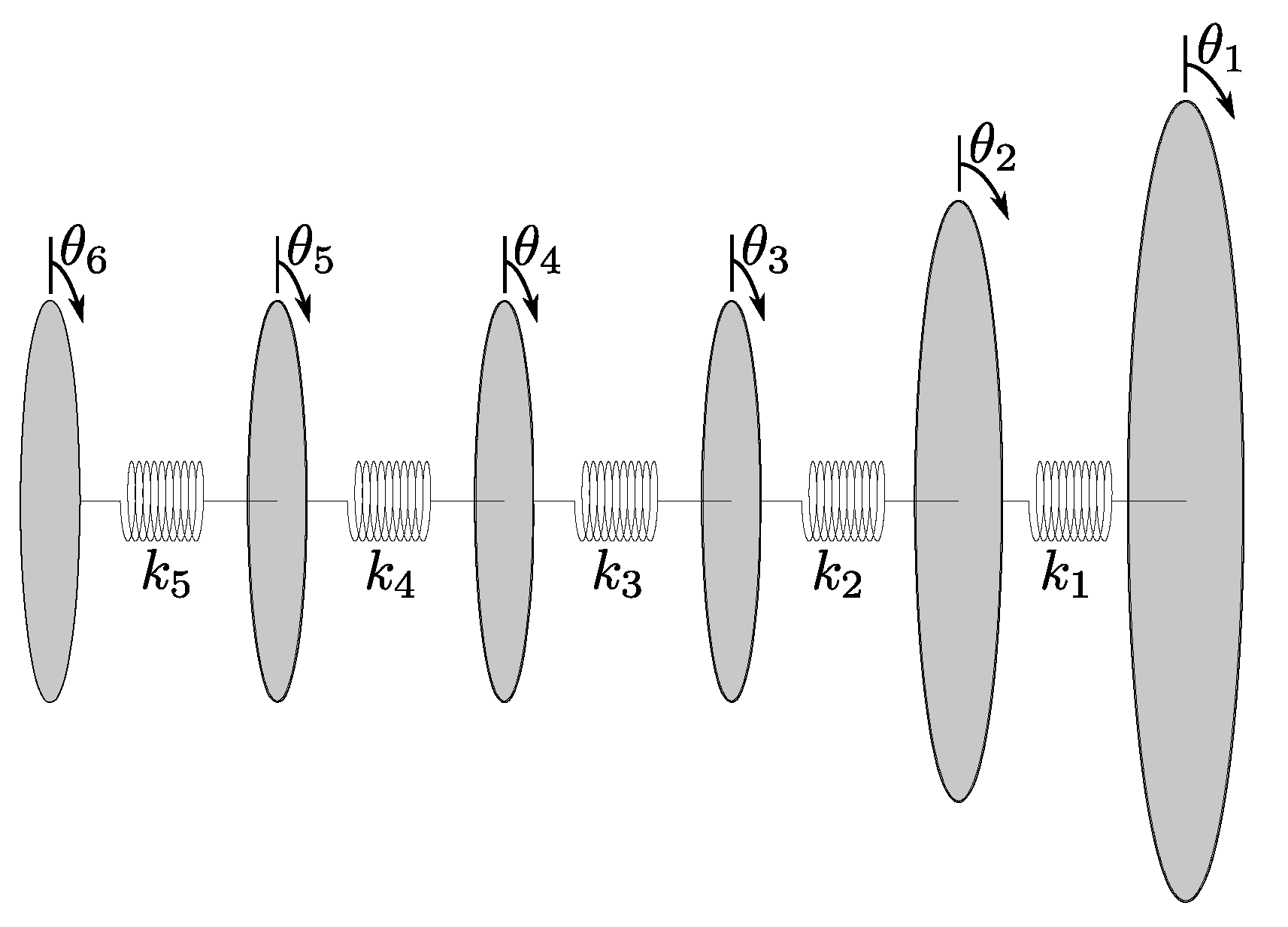
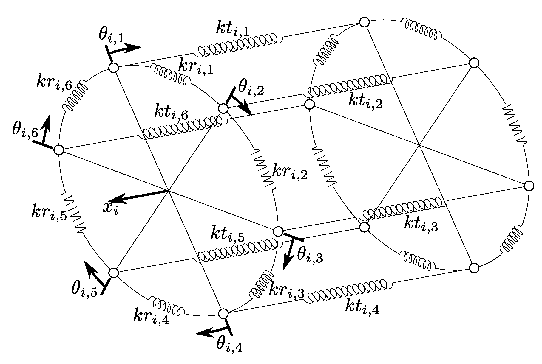
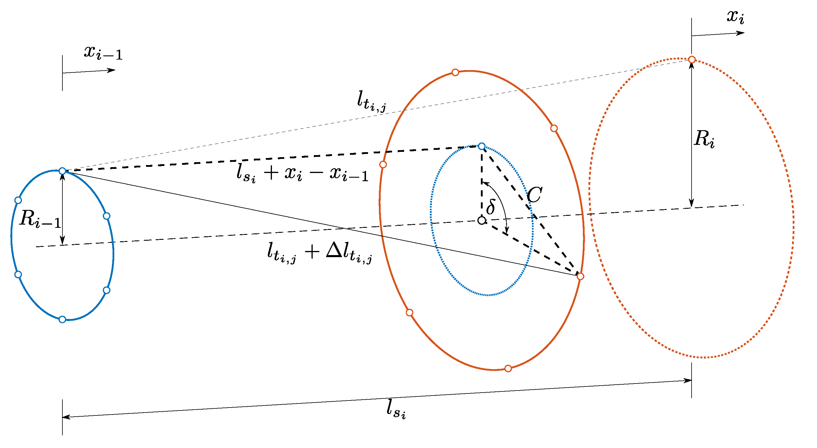
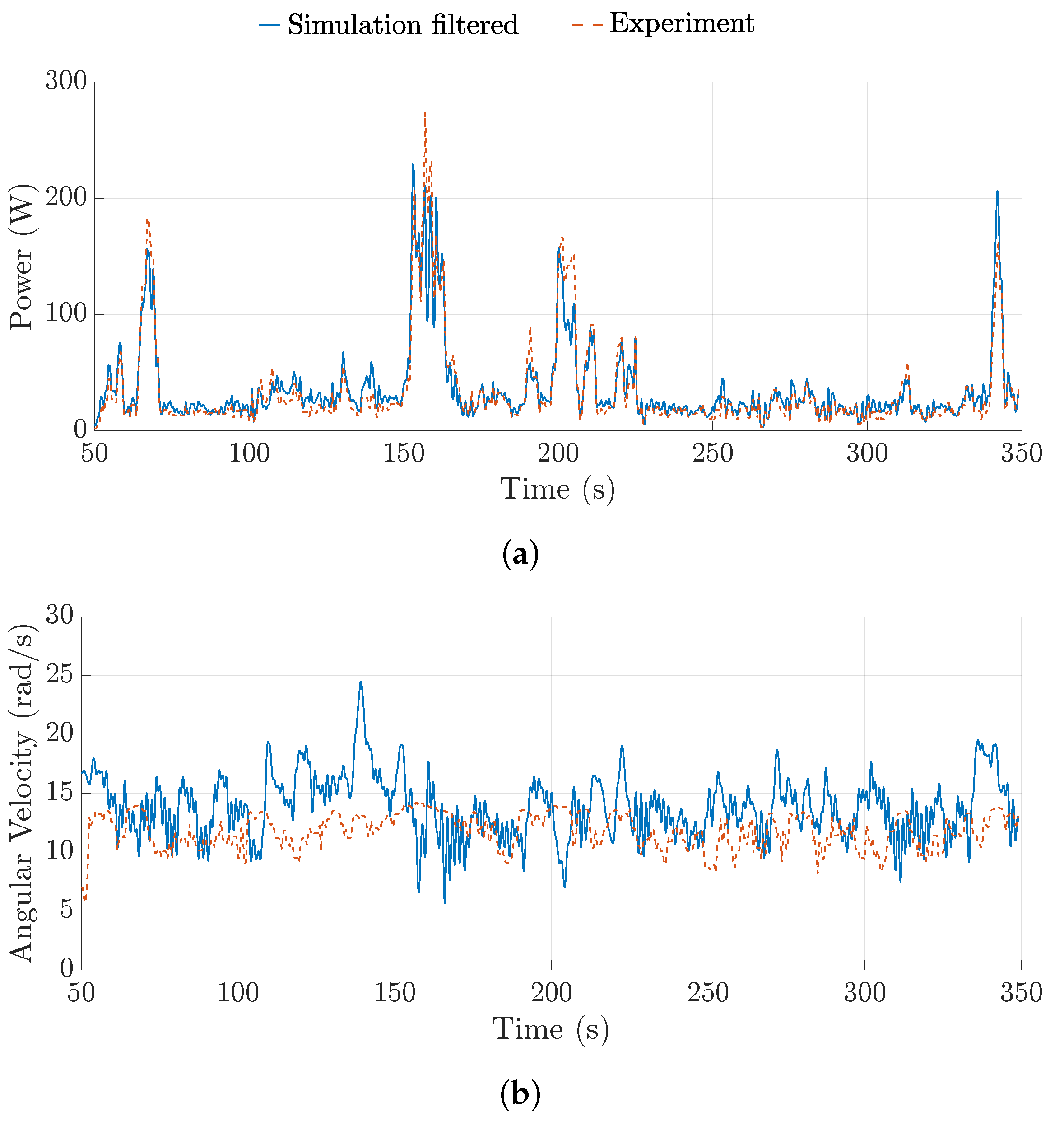
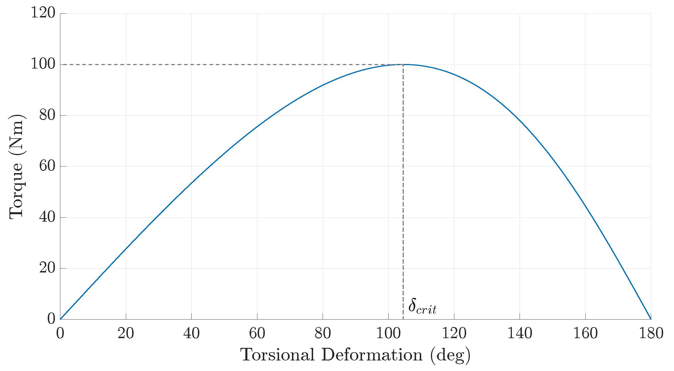
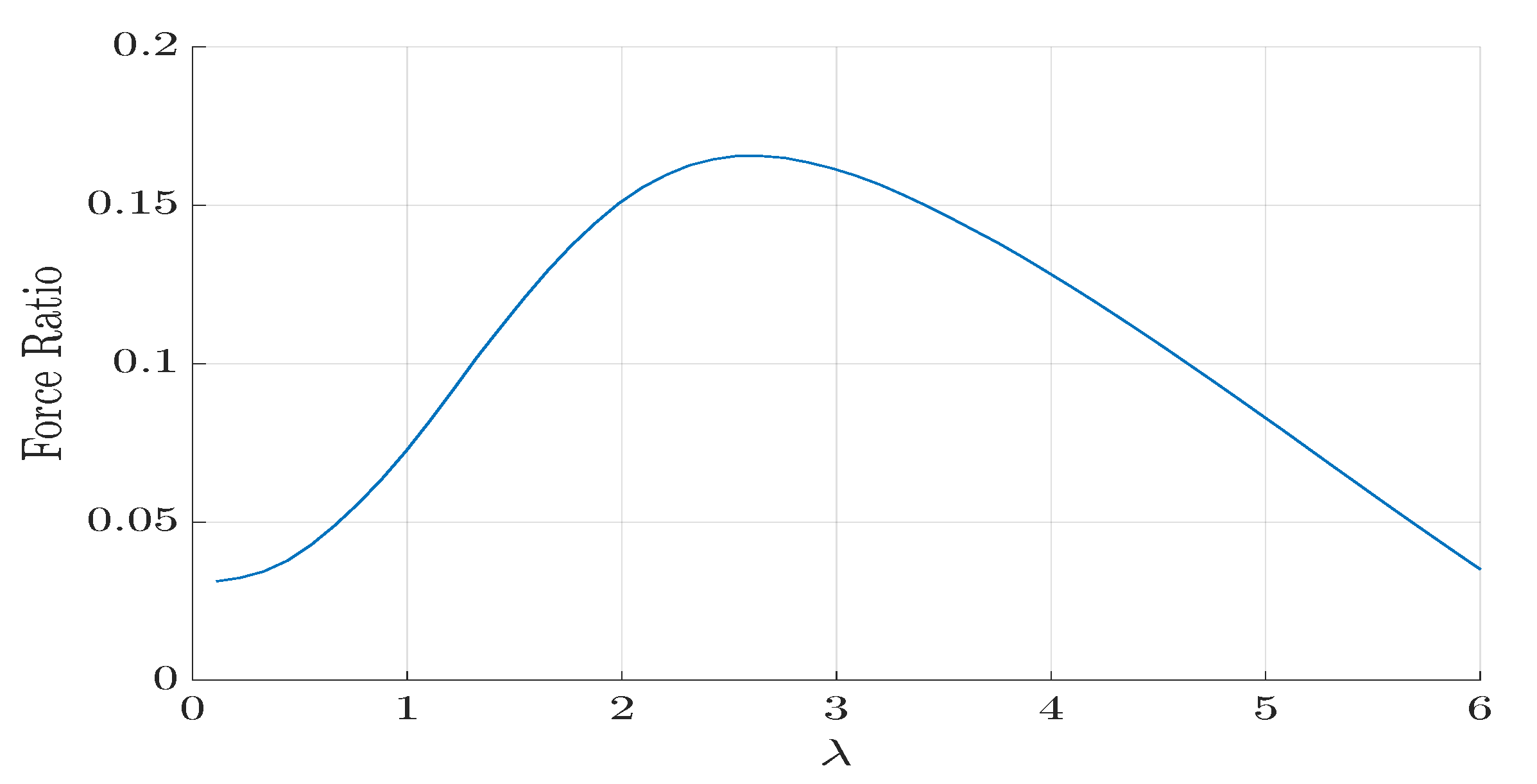
Table A1.
Pseudo code for the spring-disc TRPT representation. is the vector for the discs radii, is the vector containing the TRPT section lengths, the vector for tether lengths in each TRPT section, is the inertia matrix, the rotor torque, the rotor thrust, the rotor power, the lift kite line tension, the axial force, the torque loss due to tether drag, the torque applied to each disc, the stiffness matrix, the time step length and the vectors containing the discs rotational positions, velocities and accelerations, respectively. and are variables used within the algorithm.
| Inputs | Wind speed , TRPT geometry R and , elevation angle , initial conditions and , and generator torque |
| Line 1 | Find and |
| Line 2 | Find , and |
| Line 3 | Find , and |
| Line 4 | Find and |
| Line 5 | |
| Line 6 | |
| Line 7 | , |
| Line 8 | For each time step, i |
| Line 9 | Find , and |
| Line 10 | Find , and update |
| Line 11 | Find and |
| Line 12 | |
| Line 13 | |
| Line 14 | , |
| Line 15 | End For |
| Outputs | , , , , , , , |
Appendix A.2. Multi-Spring TRPT Modelling
The algorithm implemented to solve this multi-spring representation, for a fixed generator torque, is given in Table A2.
Table A2.
Pseudo code for the multi-spring TRPT representation. is the vector for the discs radii, is the vector containing the TRPT section lengths, the vector for tether lengths in each TRPT section, the mass and inertia matrix, the rotor torque, the rotor thrust, the rotor power, the lift kite line tension, the spring forces, the aerodynamic forces on the tethers, the force applied to each point mass, the time step length and the vectors containing the masses positions, velocities and accelerations respectively. are variables used within the algorithm.
| Inputs | Wind speed , TRPT geometry R and , elevation angle , initial conditions and , generator torque , and number of tethers . |
| Line 1 | Find and |
| Line 2 | Find , and |
| Line 3 | Find , and |
| Line 4 | Find |
| Line 5 | |
| Line 6 | |
| Line 7 | , |
| Line 8 | For each time step, i |
| Line 9 | Find , and |
| Line 10 | Find , and |
| Line 11 | Find |
| Line 12 | |
| Line 13 | |
| Line 14 | , |
| Line 15 | End For |
| Outputs | , , , , , , , , |
Appendix B. Four TRPT Configurations
Several TRPT configurations tested in the experimental campaign were used in this paper, see Figure A1 for their structures and dimensions. The main difference between them is the number of carbon-fibre rings, the diameter of the rings and the length of tethers between the rings. The ground-station wheel in versions 1, 2, and 3 has a diameter of 0.42 m, for versions 4 this was increased to a diameter of 0.63 m. W&I have found that, in general, the Daisy Kite’s TRPT configuration is less capable of transferring torsion as the distance between rings becomes larger and the ring diameter is reduced [3]. The ground-station wheel diameter was increased to allow for larger amounts of torque to be transmitted.
Figure A1.
Diagrams of TRPT iterations 1, 2, 3, and 4 used throughout this work. (a) TRPT−1; (b) TRPT−2; (c) TRPT−3; (d) TRPT−4.
Figure A1.
Diagrams of TRPT iterations 1, 2, 3, and 4 used throughout this work. (a) TRPT−1; (b) TRPT−2; (c) TRPT−3; (d) TRPT−4.

Appendix C. Comparison of Multi-Spring Model and Experimental Data
In addition to the comparison results given in Figure 16, Section 4.3.2, another four sets of field-testing data were used to validate the multi-spring TRPT model; results are shown in the following figure.
Figure A2.
Comparison of the ground station angular velocity between the multi-spring model and experimental data. (a) 20 September 2018: rigid wing, TRPT−3; (b) 27 August 2018: rigid wing, TRPT−3; (c) 5 June 2018: soft wing, TRPT−2; (d) 18 June 2017: soft wing, TRPT−1.
Figure A2.
Comparison of the ground station angular velocity between the multi-spring model and experimental data. (a) 20 September 2018: rigid wing, TRPT−3; (b) 27 August 2018: rigid wing, TRPT−3; (c) 5 June 2018: soft wing, TRPT−2; (d) 18 June 2017: soft wing, TRPT−1.

References
- Bramwell, A.R.S.; Done, G.; Blamford, D. Bramwell’s Helicopter Dynamics; Butterworth-Heinemann: Oxford, UK, 2001. [Google Scholar]
- Read, R. Windswept & Interesting Ltd. Available online: https://www.windswept-and-interesting.co.uk/ (accessed on 10 January 2020).
- Read, R. Kite Networks for Harvesting Wind Energy. In Airborne Wind Energy: Advances in Technology Development and Research; Schmehl, R., Ed.; Springer: Singapore, 2018; pp. 515–537. [Google Scholar] [CrossRef]
- Tulloch, O. Modelling and Analysis of Rotary Airborne Wind Energy Systems—A Tensile Rotary Power Transmission Design. Ph.D. Thesis, University of Strathclyde, Glasgow, UK, 2021. [Google Scholar] [CrossRef]
- Malz, E. Airborne Wind Energy—To Fly or Not to Fly? A Study on the Power Production of Airborne Wind Energy Systems and Their Integration in the Electricity Generation System. Ph.D. Thesis, Chalmers University of Technology, Göteberg, Sweden, 2020. [Google Scholar] [CrossRef]
- De Schutter, J.; Leuthold, R.; Bronnenmeyer, T.; Paelinck, R.; Diehl, M. Optimal control of stacked multi-kite systems for utility-scale airborne wind energy. In Proceedings of the 2019 IEEE 58th Conference on Decision and Control (CDC), Nice, France, 11–13 December 2019; pp. 4865–4870. [Google Scholar] [CrossRef]
- Rimkus, S.; Das, T. An application of the autogyro theory to airborne wind energy extraction. In Proceedings of the ASME 2013 Dynamic Systems and Control Conference, DSCC 2013, American Society of Mechanical Engineers (ASME), Palo Alto, CA, USA, 21–23 October 2013; Volume 3. [Google Scholar] [CrossRef] [Green Version]
- Mackertich, S.; Das, T. A quantitative energy and systems analysis framework for airborne wind energy conversion using autorotation. In Proceedings of the 2016 American Control Conference (ACC). American Automatic Control Council (AACC), Boston, MA, USA, 6–8 July 2016; pp. 4996–5001. [Google Scholar] [CrossRef]
- Rancourt, D.; Bolduc-Teasdale, F.; Bouchard, E.D.; Anderson, M.J.; Mavris, D.N. Design space exploration of gyrocopter-type airborne wind turbines. Wind Energy 2016, 19, 895–909. [Google Scholar] [CrossRef]
- Benhaïem, P.; Schmehl, R. Airborne wind energy conversion using a rotating reel system. In Airborne Wind Energy: Advances in Technology Development and Research; Schmehl, R., Ed.; Springer: Singapore, 2018; pp. 539–577. [Google Scholar] [CrossRef]
- Roberts, B.W. Quad-rotorcraft to harness high-altitude wind energy. In Airborne Wind Energy: Advances in Technology Development and Research; Schmehl, R., Ed.; Springer: Singapore, 2018. [Google Scholar] [CrossRef] [Green Version]
- Schutter, J.D.; Leuthold, R.; Diehl, M. Optimal control of a rigid-wing rotary kite system for airborne wind energy. In Proceedings of the 2018 European Control Conference (ECC), Limassol, Cyprus, 12–15 June 2018; pp. 1734–1739. [Google Scholar] [CrossRef]
- Beaupoil, C. Practical experiences with a torsion based rigid blade rotary airborne wind energy system with ground based power generation. In Proceedings of the 8th International Airborne Wind Energy Conference (AWEC2019), Glasgow, UK, 15–16 October 2019; Schmehl, R., Tulloch, O., Eds.; Delft University of Technology and University of Strathclyde: Glasgow, UK, 2019; pp. 146–147. [Google Scholar]
- Selsam, D. Selsam—Innovation in Alternative Energy. Available online: http://www.selsam.com (accessed on 4 December 2017).
- Sky WindPower. Available online: https://www.skywindpower.com (accessed on 27 March 2019).
- Ippolito, M. KiteGen Carousel. Available online: http://www.kitegen.com/en/products/kite-gen-carousel (accessed on 21 March 2021).
- Castellani, F.; Astolfi, D.; Natili, F.; Mari, F. The yawing behavior of horizontal-axis wind turbines: A numerical and experimental analysis. Machines 2019, 7, 15. [Google Scholar] [CrossRef] [Green Version]
- Micallef, D.; Kloosterman, M.; Ferreira, C.S.; Sant, T.; van Bussel, G.; Micallef, D. Comparison and validation of BEM and free wake unsteady panel model with the Mexico rotor experiment. In Proceedings of the Euromech, Madrid, Spain, 20–22 October 2009; Volume 508. Available online: http://resolver.tudelft.nl/uuid:33950a07-dbaf-492b-bfec-8833984afd2f (accessed on 21 March 2021).
- Rahimi, H.; Hartvelt, M.; Peinke, J.; Schepers, J. Investigation of the current yaw engineering models for simulation of wind turbines in BEM and comparison with CFD and experiment. J. Phys. Conf. Ser. 2016, 753, 022016. [Google Scholar] [CrossRef] [Green Version]
- Micallef, D.; Sant, T. A review of wind turbine yaw aerodynamics. In Wind Turbines; Aissaoui, A.G., Tahour, A., Eds.; IntechOpen: Rijeka, Croatia, 2016; Chapter 2. [Google Scholar] [CrossRef] [Green Version]
- Ghoreyshi, M.; Bergeron, K.; Seidel, J.; Jirasek, A.; Lofthouse, A.J.; Cummings, R.M. Prediction of aerodynamic characteristics of ram-air parachutes. J. Aircr. 2016, 53, 1802. [Google Scholar] [CrossRef]
- Hansen, C. AirfoilPrep. Available online: https://nwtc.nrel.gov/AirFoilPrep (accessed on 4 July 2020).
- Ostowari, C.; Naik, D. Post-Stall Wind Tunnel Data for NACA 44xx Series Airfoil Sections; Technical Report; Department of Aerospace Engineering, Texas A and M University: College Station, TX, USA, 1985. [Google Scholar] [CrossRef] [Green Version]
- NACA 4412 (naca4412-il) Xfoil Prediction Polar at RE=200,000 Ncrit=5. Available online: http://airfoiltools.com/polar/details?polar=xf-naca4412-il-200000-n5 (accessed on 4 April 2020).
- Manwell, J.; McGowan, J.; Rogers, A. Wind Energy Explained; Wiley: Hoboken, NJ, USA, 2002. [Google Scholar]
- Jonkman, B.; Kilcher, L. TurbSim User’s Guide: Version 1.06. 00; National Renewable Energy Laboratory: Golden, CO, USA, 2012.
- IEC 61400-1; Wind Turbines–Part 1: Design Requirements. IEC: Geneva, Switzerland, 2005.
- Tulloch, O.; Amiri, A.K.; Yue, H.; Feuchtwang, J.; Read, R. Tensile rotary power transmission model development for airborne wind energy systems. J. Phys. Conf. Ser. 2020, 1618, 032001. [Google Scholar] [CrossRef]
- Chopra, A.K. Dynamics of Structures Theory and Applications to Earthquake Engineering; Prentice Hall: Hoboken, NJ, USA, 1995. [Google Scholar] [CrossRef]
- Zanon, M.; Gros, S.; Andersson, J.; Diehl, M. Airborne wind energy based on dual airfoils. IEEE Trans. Control Syst. Technol. 2013, 21, 1215–1222. [Google Scholar] [CrossRef] [Green Version]
- Dunker, S. Tether and bridle line drag in airborne wind energy applications. In Airborne Wind Energy: Advances in Technology Development and Research; Schmehl, R., Ed.; Springer: Singapore, 2018; pp. 29–56. [Google Scholar] [CrossRef]
- Bootle, W. Forces on an inclined circular cylinder in supercritical flow. AIAA J. 1971, 9, 514–516. [Google Scholar] [CrossRef]
- DSM. Dyneema. Available online: https://www.dsm.com/products/dyneema/en_GB/home.html (accessed on 17 February 2020).
- Carbon Fibre Profiles. Available online: https://www.carbonfibreprofiles.com/ (accessed on 17 February 2020).
- Sanborn, B.; Dileonardi, A.M.; Weerasooriya, T. Tensile properties of dyneema SK76 single fibers at multiple loading rates using a direct gripping method. J. Dyn. Behav. Mater. 2014, 1, 4–14. [Google Scholar] [CrossRef]
Figure 1.
System configuration of the Daisy-Kite AWE system.

Figure 2.
Block diagram of the rotary AWES (key variables indicated).

Figure 3.
Representation of a single TRPT section within the Daisy Kite system [28].
Figure 3.
Representation of a single TRPT section within the Daisy Kite system [28].

Figure 4.
Schematic of the spring-disc TRPT representation. Each ring is described by a moment of inertia, J, and the multiple tethers in each section are replaced by a single torsional spring of stiffness k. Disc 6, on the left hand side of the schematic, represents the ground-station end of the TRPT.

Figure 5.
Schematic of the multi-spring TRPT representation. Each ring is represented by ( in this design) linear springs with stiffness and the tethers by linear springs with stiffness . The number of degrees of freedom for a single ring is .
Figure 5.
Schematic of the multi-spring TRPT representation. Each ring is represented by ( in this design) linear springs with stiffness and the tethers by linear springs with stiffness . The number of degrees of freedom for a single ring is .

Figure 6.
Diagram showing the change in tether length, , of the j-th tether within the i-th TRPT section.
Figure 6.
Diagram showing the change in tether length, , of the j-th tether within the i-th TRPT section.

Figure 7.
Diagram showing the aerodynamic force on a tether point.

Figure 8.
Image of a rigid rotor Daisy Kite prototype undergoing field tests (August 2019).

Figure 9.
TRPT laboratory test set-up and results, 30 kg axial load case. (a) TRPT section lab testing with two wheels; (b) Lab testing results compared to calculated torsional deformation.
Figure 9.
TRPT laboratory test set-up and results, 30 kg axial load case. (a) TRPT section lab testing with two wheels; (b) Lab testing results compared to calculated torsional deformation.

Figure 10.
Steady-state power coefficient against tip speed ratio, Daisy Kite configuration comparisons using spring-disc model. (a) Rigid and soft wings; (b) 4° & 0° pitched rigid wings; (c) TRPT–3 and 4; (d) 3 and 6 blades.
Figure 10.
Steady-state power coefficient against tip speed ratio, Daisy Kite configuration comparisons using spring-disc model. (a) Rigid and soft wings; (b) 4° & 0° pitched rigid wings; (c) TRPT–3 and 4; (d) 3 and 6 blades.

Figure 11.
Power coefficient against tip speed ratio for various Daisy Kite configurations using the steady-state spring-disc model compared to experimental data. (a) Soft wing TRPT−1; (b) Soft wing TRPT−2; (c) Soft wing TRPT−3; (d) Rigid wing TRPT−3; (e) Rigid wing TRPT−4; (f) Rigid 6−wing TRPT−5.
Figure 11.
Power coefficient against tip speed ratio for various Daisy Kite configurations using the steady-state spring-disc model compared to experimental data. (a) Soft wing TRPT−1; (b) Soft wing TRPT−2; (c) Soft wing TRPT−3; (d) Rigid wing TRPT−3; (e) Rigid wing TRPT−4; (f) Rigid 6−wing TRPT−5.

Figure 12.
Power spectral density of the ground station angular velocity for the spring-disc model with and without a low pass filter applied.
Figure 12.
Power spectral density of the ground station angular velocity for the spring-disc model with and without a low pass filter applied.

Figure 13.
Comparison between the spring-disc model with a low pass filter and experimental data. (a) Power output comparison; (b) Angular velocity comparison.
Figure 13.
Comparison between the spring-disc model with a low pass filter and experimental data. (a) Power output comparison; (b) Angular velocity comparison.

Figure 14.
Results from the multi-spring representation comparing rigid and flexible carbon fibre rings within the TRPT.
Figure 14.
Results from the multi-spring representation comparing rigid and flexible carbon fibre rings within the TRPT.

Figure 15.
Power spectral density of the ground-station rotational speed for the multi-spring model with and without a low pass filter applied compared to the experimental data.
Figure 15.
Power spectral density of the ground-station rotational speed for the multi-spring model with and without a low pass filter applied compared to the experimental data.

Figure 16.
Comparison between experimental data and multi-spring model with a low pass filter. (a) Power output comparison; (b) Angular velocity comparison.
Figure 16.
Comparison between experimental data and multi-spring model with a low pass filter. (a) Power output comparison; (b) Angular velocity comparison.

Figure 17.
Response of angular velocity of the rotor to changes in torque and axial tension for the spring-disc and multi-spring models, TRPT length 30 m, wind speed of 8 m/s. (a) Response to a change in torque; (b) Response to a change in axial tension.
Figure 17.
Response of angular velocity of the rotor to changes in torque and axial tension for the spring-disc and multi-spring models, TRPT length 30 m, wind speed of 8 m/s. (a) Response to a change in torque; (b) Response to a change in axial tension.

Figure 18.
Amount of torque transmitted against the torsional deformation for a single TRPT section of the Daisy Kite.
Figure 18.
Amount of torque transmitted against the torsional deformation for a single TRPT section of the Daisy Kite.

Figure 19.
Torsional stiffness variation with torsional deformation for a single TRPT section of the Daisy Kite.
Figure 19.
Torsional stiffness variation with torsional deformation for a single TRPT section of the Daisy Kite.

Figure 20.
Critical torsional deformation for different tether-length-to-ring-radius ratios.

Figure 21.
Force ratio against torsional deformation.

Figure 22.
Force ratio against the length-to-radius ratio.

Figure 23.
Variation in with system elevation angle.

Figure 24.
Effect of wing pitch angle on vs. curve.

Figure 25.
Effect of blade length on rotor power output and . (a) ; (b) Power output.

Figure 26.
Effect of TRPT torsional deformation on the torque loss due to tether drag.

Figure 27.
Optimised rotor design compared to the rotor used in prototype configuration 8. (a) vs. ; (b) Power output.
Figure 27.
Optimised rotor design compared to the rotor used in prototype configuration 8. (a) vs. ; (b) Power output.

Figure 28.
Force ratio against the tip speed ratio for the optimised Daisy Kite rotor.

Figure 29.
Maximum force ratio and TRPT efficiency versus TRPT radius.

Figure 30.
Power output for the optimised Daisy Kite rotor for different TRPT lengths.

Table 1.
Five experiments used for comparison with the mathematical representations.
| Case | Test Date | Wing | TRPT | Wind Speed (m/s) | Power Output (w) | 1st Natural Frequency (Hz) |
|---|---|---|---|---|---|---|
| 1 | 8 September 2019 | Rigid | 4 | 5.3 | 35 | 0.74 |
| 2 | 20 September 2018 | Rigid | 3 | 6.1 | 50 | 1.43 |
| 3 | 27 August 2018 | Rigid | 3 | 2.7 | 10 | 0.73 |
| 4 | 6 May 2018 | Soft | 2 | 5.8 | 10 | 1.47 |
| 5 | 18 June 2017 | Soft | 1 | 5.5 | 15 | 1.52 |
Table 2.
Comparison of rotor velocity between the multi-spring and spring-disc models in RMSE.
| Wind Speed (m/s) | Change in Torque RMSE | Change in Tension RMSE |
|---|---|---|
| 6 | 0.056 | 0.332 |
| 8 | 0.038 | 0.271 |
| 10 | 0.019 | 0.186 |
| 12 | 0.019 | 0.119 |
Table 3.
Comparison of torque loss and transmission efficiency of the tether-drag models.
| Models | Torque Loss (Nm) | TRPT–4 Efficiency (%) |
|---|---|---|
| Simple tether-drag model | 7.6 | 83.2 |
| Improved tether-drag model ( neglected) | 4.9 | 89.2 |
| Improved tether-drag model | 5.1 | 88.6 |
Table 4.
Proposed Daisy Kite system design.
| Rotor Radius | Blade Length | TRPT Radius | TRPT Section Length | Elevation Angle | TRPT Total Length | Tip Speed Ratio |
|---|---|---|---|---|---|---|
| 2.22 m | 1.4 m | 0.5 m | 1.25 m | 18.5 | 190 m | 3.5 |
Disclaimer/Publisher’s Note: The statements, opinions and data contained in all publications are solely those of the individual author(s) and contributor(s) and not of MDPI and/or the editor(s). MDPI and/or the editor(s) disclaim responsibility for any injury to people or property resulting from any ideas, methods, instructions or products referred to in the content. |
© 2023 by the authors. Licensee MDPI, Basel, Switzerland. This article is an open access article distributed under the terms and conditions of the Creative Commons Attribution (CC BY) license (https://creativecommons.org/licenses/by/4.0/).
Share and Cite
MDPI and ACS Style
Tulloch, O.; Yue, H.; Kazemi Amiri, A.M.; Read, R. A Tensile Rotary Airborne Wind Energy System—Modelling, Analysis and Improved Design. Energies 2023, 16, 2610. https://0-doi-org.brum.beds.ac.uk/10.3390/en16062610
AMA Style
Tulloch O, Yue H, Kazemi Amiri AM, Read R. A Tensile Rotary Airborne Wind Energy System—Modelling, Analysis and Improved Design. Energies. 2023; 16(6):2610. https://0-doi-org.brum.beds.ac.uk/10.3390/en16062610
Chicago/Turabian StyleTulloch, Oliver, Hong Yue, Abbas Mehrad Kazemi Amiri, and Roderick Read. 2023. "A Tensile Rotary Airborne Wind Energy System—Modelling, Analysis and Improved Design" Energies 16, no. 6: 2610. https://0-doi-org.brum.beds.ac.uk/10.3390/en16062610
Note that from the first issue of 2016, this journal uses article numbers instead of page numbers. See further details here.