Simulation of Internal Manifold-Type Molten Carbonate Fuel Cells (MCFCs) with Different Operating Conditions

Abstract

Molten carbonate fuel cells (MCFCs) use molten carbonate as an electrolyte. MCFCs operate at high temperatures and have the advantage of using methane as a fuel because they can use nickel-based catalysts. We analyzed the performance of an internal manifold-type MCFC, according to operating conditions, using computational fluid dynamics. Different conditions were used for the external and internal reforming-type MCFCs. Flow directions, gas utilization, and operating temperatures were used as the conditions for the external reforming-type MCFCs. The S/C ratio and reforming area were used as the conditions for internal reforming-type MCFCs. A simulation model was developed, considering gas transfer, reforming reaction, and heat transfer. The simulation results of external reforming-type MCFCs showed similar pressure drops in all flow directions. As the gas utilization decreased, the temperature decreased, but the performance increased. The performance improved with increasing operating temperatures. The simulation results for the internal reforming-type MCFCs showed that more hydrogen was produced as the S/C ratio decreased, and the performance increased accordingly. More hydrogen was produced as the reforming area increased. However, similar performance was obtained when the reforming area contained the same active area. The external and internal reforming-type MCFCs were compared under the same conditions. The efficiency of the external reforming-type MCFCs is higher than that of the internal reforming-type MCFCs.

1. Introduction

Recently, various technologies related to hydrogen production and carbon neutrality have been studied as interest in environmental issues has increased. Fuel cells are energy-conversion systems that convert chemical energy into electrical energy. Theoretically, electricity can be produced continuously when hydrogen is supplied. Therefore, fuel cells are simpler and more efficient in terms of energy conversion than internal combustion engines [1]. Fuel cells are classified according to the type of electrolyte used.

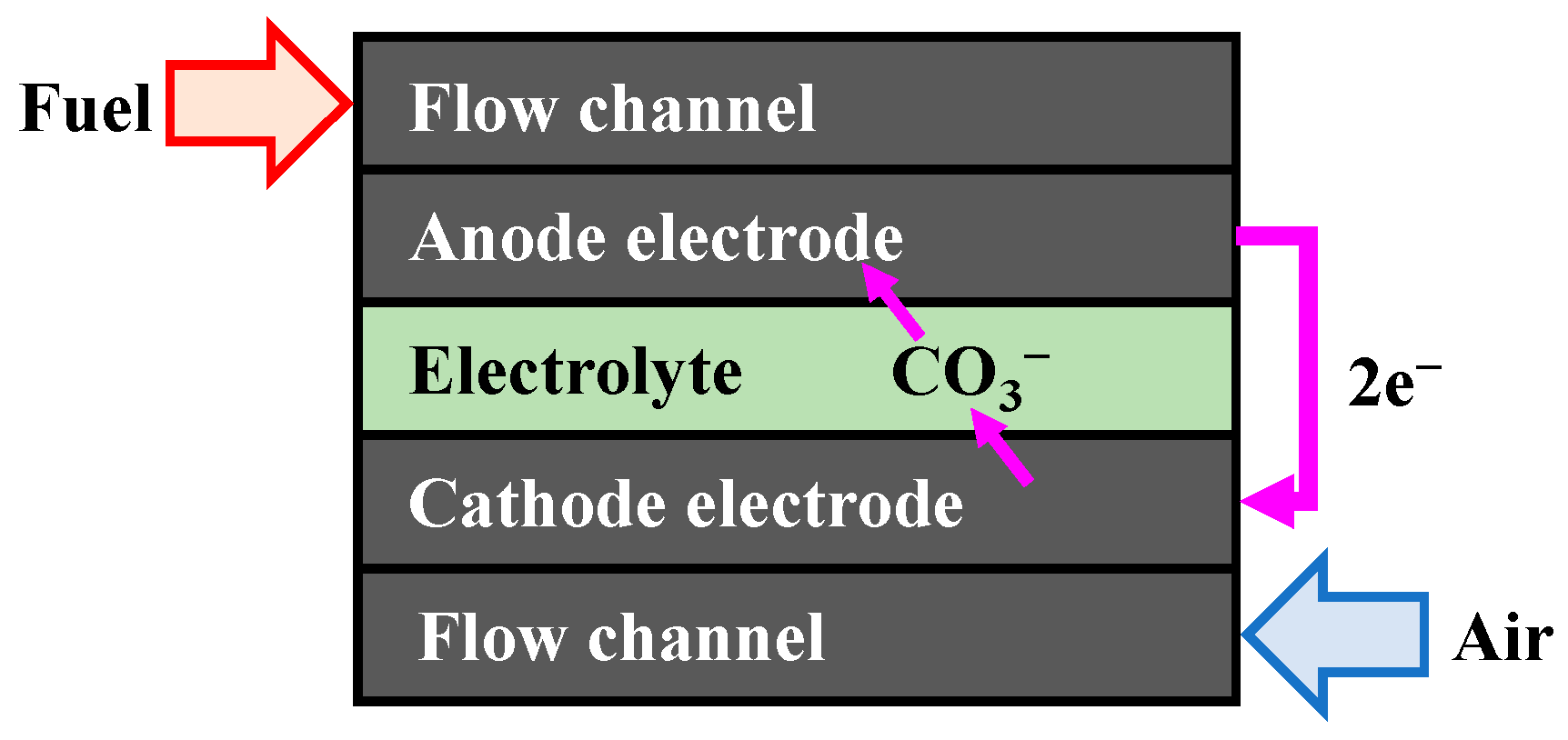
Molten carbonate fuel cells (MCFCs) use carbonate as an electrolyte. In addition, a nickel-based catalyst can be used instead of a noble metal catalyst, such as platinum, since it operates at a high temperature of 600 °C or more. Thus, it is economical because not only can hydrogen be used directly, but methane can also be used as a fuel. In MCFCs, half-reactions occur at the anode and cathode. At the anode, hydrogen and carbonate combine via an oxidation reaction to produce water, carbon dioxide, and electrons. The generated electrons then move to the cathode through an external circuit. The transferred electrons and oxygen combine to generate carbonate ions, which move to the anode through the electrolyte at the cathode. Figure 1 is a schematic diagram of the electrochemical reaction in MCFC. And the reactions at the anode and cathode are as follows:

$$Anode:H_2+C{O}_3^{2-}\to H_{2}O+C{O}_2+2e^{-}$$

(1)

$$Cathode:C{O}_2+\frac{1}{2}{O}_2+2e^{-}\to C{O}_3^{2-}$$

(2)

Although numerous studies have been conducted on fuel cells, there are limitations in the analysis of various experimental results. Accordingly, computational fluid dynamics (CFD) is widely used to predict the performance of fuel cells and analyze the distribution of temperature, diffusion, and current density.

In the field of fuel cell research, CFD is used to predict performance according to design parameters and operating conditions. Lee et al. [2] designed a cell frame structure in a 100 cm² unit cell of MCFCs using CFD. The maximum temperature decreases as the height of the cell frame increases. In addition, the optimal parameters for reducing the temperature and uniformly injecting gas were derived. Yu et al. [3] studied the sizes and flow directions of MCFCs. Similar temperatures occurred in all flow directions when the particle size increased beyond a certain value, and the maximum temperature decreased according to the amount of air at the cathode. Kim et al. [4] compared the fuel cell characteristics according to the flow direction in large-area MCFCs of 1 m². The most stable operation was possible when the flow direction of the anode side and that of the cathode side were the same.

Furthermore, not only the electrochemical reaction, but also the reforming reaction of fuel cells can be predicted using CFD. Accordingly, studies on internal reforming-type MCFCs are also being conducted. Kim et al. [5] compared the internal and external reforming-type MCFCs. Stable operation is possible because the internal reforming-type MCFC generates a relatively uniform current density and temperature distribution under the condition of using the cross-flow. Jung et al. [6] analyzed the performance according to the operating conditions in 100 cm² direct internal reforming-type MCFCs. The mole fraction and performance were compared according to the S/C ratio, operating temperature, and gas utilization. A similar performance was obtained under all S/C ratio conditions; however, the performance increased as the operating temperature increased and the gas utilization decreased.

Meanwhile, it is possible to analyze the performance of a fuel cell according to the type and shape of the manifold using CFD. Kim et al. [7] predicted and characterized the performance of internal manifold-type MCFCs through heat and fluid simulations. They confirmed that the bypass effect occurred in an area without an electrode surface. Zhao et al. [8] constructed a 40-cell stack comprising an external manifold using CFD and analyzed the flow and pressure changes. It was found that a higher manifold depth and numerous inlets could aid in the gas flow distribution owing to the low flow rate.

In this study, the current densities, temperatures, pressures, and performances of external and internal reforming-type MCFCs under various operating conditions were analyzed using CFD. In the external reforming-type MCFC, the results were derived according to the flow direction, gas utilization, and operating temperature. For the internal reforming-type MCFCs, the results were derived according to the S/C ratio and reforming area. Finally, the internal and external reforming-type MCFCs were compared under the suggested conditions.

2. Simulation Model

2.1. The Governing Equations of MCFCs

The cell voltage (V_cell) at the electrode was obtained by subtracting the cell resistance and polarization resistance losses from the Nernst potential, as shown in Equation (3). The Nernst potential (E_Nernst) is a model that converts chemical energy into electrical energy. The Nernst potential was determined from the difference between the standard potential (E⁰) and the concentrations of the reactants and products of the MCFCs, as shown in Equation (4), where the standard potential was controlled by the operating temperature of the MCFCs, as shown in Equation (5) [9].

$$V_{cell}^{x,y}=E_{Nernst}^{x,y}-i^{x,y}(R_{Anode}^{x,y}+R_{Cathode}^{x,y}+R_{Ohmic}^{x,y})$$

(3)

$$E_{Nernst}=E^0+\frac{RT}{2F}\ln \left(\frac{P_{H_{2_{Anode}}}\sqrt{P_{O_{2_{Cathode}}}}}{P{H}_2{O}_{Anode}}\frac{P_{C{O}_{2_{Cathode}}}}{P_{C{O}_{2_{Anode}}}}\right)$$

(4)

$$E^0=-\frac{\Delta G}{2F}=-243730+48.996\times T+2.474\times {10}^{-3}\times T^2$$

(5)

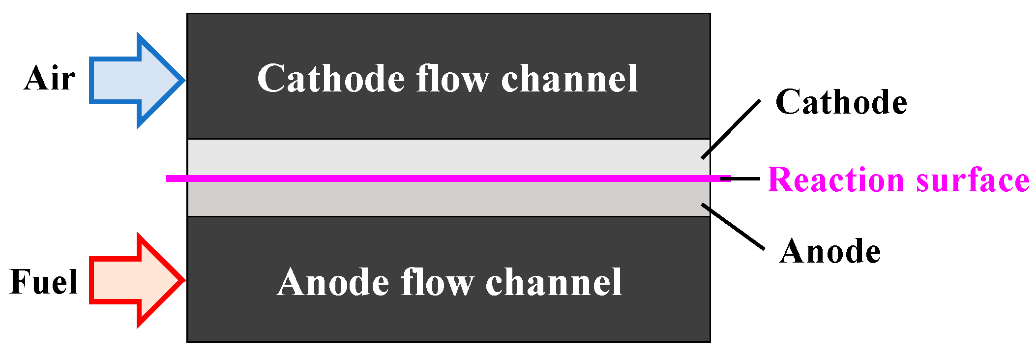
The anode resistance (R_Anode), cathode resistance (R_Cathode), and ohmic resistance (R_Ohmic) in the MCFC used Yuh and Selman’s model, which expresses the carbonate distribution between the electrode and electrolyte [10]. The model was controlled by the operating temperature and concentration of the species, as described below. The electrochemical reaction is generated in the electrolyte, but in this study, a reaction surface existing between the anode and cathode is assumed instead of the carbonate electrolyte as shown in Figure 2.

$$R_{ohmic}=0.5\times {10}^{-4}\exp \left[3016\left(\frac{1}{T}-\frac{1}{923}\right)\right]$$

(6)

$$R_{Anode}=2.27\times {10}^{-9}\exp \left(\frac{6435}{T}\right)P_{H_2}^{-0.42}{P}_{C{O}_2}^{-0.17}{P}_{H_{2}O}^{-1.0}$$

(7)

$$R_{Cathode}=7.505\times {10}^{-10}\times \exp \left(\frac{9289}{T}\right)P_{O_2}^{-0.43}{P}_{C{O}_2}^{-0.09}$$

(8)

2.2. Internal Manifold Type MCFCs

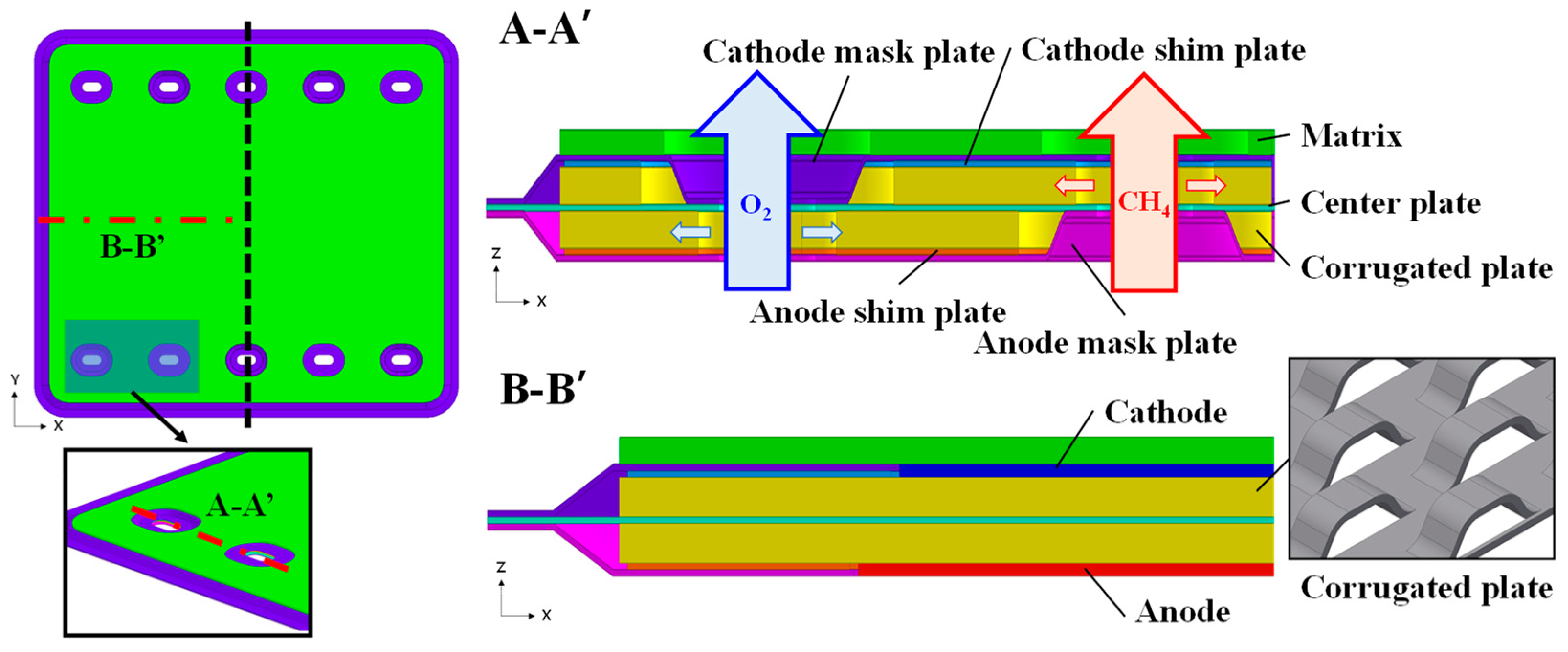
The internal manifold-type MCFCs shown in Figure 3 were used. Internal manifold-type MCFCs have a separate flow channel in which gas is supplied to the anode and cathode inside the stack. In addition, this structure has the advantage of the absence of gas-tightness problems in the manifold manufacturing stage. The internal manifold-type MCFCs used in this study have five inlets and outlets. Hydrogen passes through two inlets to three outlets, and oxygen passes through three inlets to two outlets.

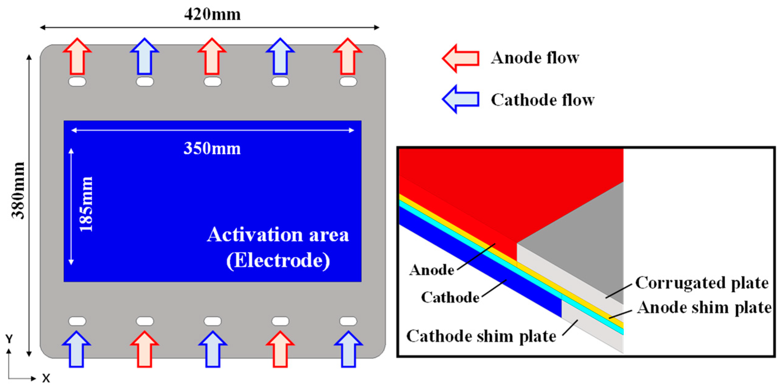
Meanwhile, not all parts of the internal manifold-type MCFCs were considered in the simulation. As shown in Figure 4, a simulation model was developed using only the anode, cathode, corrugated plate, and shim plate. The anode and cathode had a rectangular shape, with a width of 350 mm and length of 185 mm. The corrugated and shim plates were 420 mm wide and 380 mm long, respectively. The thickness of the corrugated plate was 1.78 mm and that of the shim plate was 0.3 mm.

Generally, the required flow rates of fuel and air in a fuel cell can be quantitatively determined. As shown in Equation (9), the required oxygen flow rate is calculated using the Faraday constant, reaction area, and target current density. The airflow rate was then derived from the mole fraction of oxygen and the gas utilization rate.

$$\begin{array}{c}Flow rate\hfill \\ =\frac{Current density\times Acitve area}{Faraday constant\times Number of electrons\times Mole fraction of O_2 or H_2\times Gas utilization } \left(\frac{{\mathrm{m}}^3}{\mathrm{s}}\right) \hfill \end{array}$$

(9)

Unlike at the cathode, a reforming reaction occurred at the anode. Therefore, the fuel flow rate should be calculated considering the reforming reactions of the gas mixture. The required hydrogen flow rate was derived using Equation (9). The flow rate of the fuel was then determined from the volume ratio of the gas mixture in the equilibrium and initial states. Gas was constantly injected into the corrugated plate.

The operating pressure is assumed to be 1 atm. Therefore, the density (ρ) of the chemical species in the ideal gas state was derived using Equation (10). In addition, Dalton’s law was used to determine the density of the mixed gas (ρ_mix), which is given by Equation (11) [11].

$$\rho =\frac{P}{RT} \left(\frac{\mathrm{k}\mathrm{g}}{{\mathrm{m}}^3}\right)$$

(10)

$${\rho }_{mix}=\frac{P{{\displaystyle \sum }}_{i=1}^n{X}_i{M}_i}{RT} \left(\frac{\mathrm{k}\mathrm{g}}{{\mathrm{m}}^3}\right)$$

(11)

The heat capacity was determined based on the change in temperature. Therefore, the heat capacity (C_p) according to the temperature of each chemical species was derived using the 4th order function in Equation (12), which is composed of only the temperature function. In addition, the heat capacity of the mixed gas (C_Pmix) was calculated by multiplying the heat capacity by the molar fraction of each chemical species. The heat capacity parameters for each chemical species are listed in

Table A1. Parameters of heat capacity according to chemical species [17].

Species	Parameters
	A	B	C (×10−5)	D (×10−8)	E (×10−12)	Tmin (°C)	Tmax (°C)
H2	25.399	0.020	−3.854	3.188	−8.758	523.15	1773.15
N2	29.342	−0.003	1.007	−0.431	0.259	323.15	1773.15
O2	29.526	−0.008	3.808	−0.326	8.860	323.15	1773.15
CO	29.556	−0.006	2.130	−1.222	2.261	333.15	1773.15
CO2	27.437	0.042	−1.955	0.399	−0.298	323.15	5273.15
H2O	33.933	−0.008	2.990	−0.178	0.369	373.15	1773.15
CH4	34.942	−0.039	19.184	−15.303	39.320	323.15	1773.15

, and the heat capacity of the gas mixture is given by Equation (13).

$$C_p=A+BT+C{T}^2+D{T}^3+E{T}^4 \left(\frac{\mathrm{J}}{\mathrm{m}\mathrm{o}\mathrm{l}·\mathrm{K}}\right)$$

(12)

$$C_{P_{mix}}={\displaystyle \sum }_{i=1}^n{X}_i{C}_{Pi}\left(T\right) \left(\frac{\mathrm{J}}{\mathrm{m}\mathrm{o}\mathrm{l}·\mathrm{K}}\right)$$

(13)

2.3. Determination of Gas Transfer

The cathode and anode were divided into gas-diffusion and catalyst layers. In particular, the energy transfer by gas molecules is generated by the interactions between the molecules in the gas-diffusion layer. Therefore, the momentum, heat, and mass transfers of the gas mixture must be considered in the gas diffusion layer.

Mass transfer uses Fick’s law, based on the concentration gradient and diffusion coefficient between chemical species. The diffusion coefficient of each chemical species (D_ij) was calculated using Equation (14). The diffusion coefficient was determined using the critical temperature (T_ci,j), critical pressure (P_ci,j), and molecular weight (M_ci,j). Different mass transfers occurred in the corrugated plates and electrodes. Thus, the diffusion coefficient of the corrugated plate was determined using the mixture rule (D_mix,i) in Equation (15) [12].

Table A2. Molecular weight, critical temperature, and critical pressure, according to chemical species [18].

Species	Molecular Weight (g/mol)	Critical Temperature (°C)	Critical Pressure (atm)
H2 (Nonpolar)	2.0	306.15	12.8
N2 (Nonpolar)	28.0	399.35	33.5
O2 (Nonpolar)	32.0	427.55	49.7
CO (Polar)	28.0	406.05	34.5
CO2 (Nonpolar)	44.0	577.35	72.8
H2O (Polar)	18.0	920.45	217.5
CH4 (Nonpolar)	16.0	463.55	45.3
Nonpolar + Nonpolar		Nonpolar + Polar
a	b	a	b
0.0002745	1.823	0.000364	2.334

lists the parameters required to calculate the diffusion coefficient of each chemical species.

Permeation was hindered by the walls of the small pores because the electrodes were composed of a porous medium. Therefore, the Knudsen diffusion coefficient (D_Kn,i) should be considered according to the porosity of the electrode using Equation (16). Subsequently, the effective diffusion coefficient for the electrode was derived using the Knudsen diffusion coefficient and the diffusion coefficient of the gas mixture. The effective diffusion coefficient (D_i^eff) is given by Equation (17) [13]:

$$D_{ij}=\frac{a{\left(\frac{T}{\sqrt{T_{ci}{T}_{cj}}}\right)}^b{\left(P_{ci}{P}_{cj}\right)}^{\frac{1}{3}}{\left(T_{ci}{T}_{cj}\right)}^{\frac{5}{12}}{\left(\frac{1}{M_i}+\frac{1}{M_j}\right)}^{\frac{1}{2}}}{P} \left(\frac{{\mathrm{m}}^2}{\mathrm{s}}\right)$$

(14)

$$D_{mix,i}=\frac{1-x_i}{{{\displaystyle \sum }}_{j\ne i}^N{x}_j/D_{ij}} \left(\frac{{\mathrm{m}}^2}{\mathrm{s}}\right)$$

(15)

$$D_{Kn,i}=\frac{1}{3}{r}_{pore}\sqrt{\frac{8RT}{2\pi M_i}} \left(\frac{{\mathrm{m}}^2}{\mathrm{s}}\right)$$

(16)

$$D_i^{eff}=\frac{\epsilon }{\tau }\left(\frac{D_{mix,i}{D}_{Kn,i}}{D_{mix,i}+D_{Kn,i}}\right) \left(\frac{{\mathrm{m}}^2}{\mathrm{s}}\right)$$

(17)

Momentum transfer is based on Newton’s law and the velocity gradient and viscosity coefficient between chemical species. The viscosity coefficient of each chemical species ($\mu$) was calculated using Sutherland’s law in Equation (18), which expresses gas dynamics as a function of temperature. Wilke’s mixture rule in Equation (19) was then used for the viscosity coefficient of the gas mixture ($\mu$_mix,i), where the dimensionless constant (ϕ_ij) can be determined as the molar mass and viscosity coefficient between the species, as shown in Equation (20). The Sutherland constants (C) for each chemical species are presented in

Table A3. Parameters of viscosity, according to species [19].

Species	Reference Viscosity (×10−5 kg/m/s)	Sutherland’s Constant	Reference Temperature (°C)
H2	0.840	71	546.3
N2	1.661	104	546.3
O2	1.920	123	546.3
CO	1.680	100	546.3
CO2	1.380	254	546.3
H2O	0.899	961	546.3
CH4	1.020	164	546.3

.

$$\mu ={\mu }_0\frac{T_0+C}{T+C}{\left(\frac{T}{T_0}\right)}^{\frac{3}{2}}\left(\frac{\mathrm{k}\mathrm{g}}{\mathrm{m}·\mathrm{s}}\right)$$

(18)

$${\mu }_{mix,i}=\frac{x_i{\mu }_i}{{{\displaystyle \sum }}_{j\ne i}^N{x}_j{\varphi }_{ij}}\left(\frac{\mathrm{k}\mathrm{g}}{\mathrm{m}·\mathrm{s}}\right)$$

(19)

$${\varphi }_{ij}=\frac{1}{\sqrt{8}}{\left(1+\frac{M_i}{M_j}\right)}^{-\frac{1}{2}}{\left[1+{\left(\frac{{\mu }_i}{{\mu }_j}\right)}^{\frac{1}{2}}{\left(\frac{M_i}{M_j}\right)}^{\frac{1}{4}}\right]}^2$$

(20)

The heat transfer uses Fourier’s law, based on the temperature gradient and thermal conductivity of the chemical species. For the thermal conductivity of each chemical species (k_T), a quadratic equation expressing only a function of temperature was used, as shown in Equation (21). The conductivity of the gas mixture was determined using Wilke’s mixture rule, as shown in Equation (19).

Table A4. Parameters of thermal conductivity, according to species [20].

Species	Parameters
	A	B (×10−5)	C (×10−8)	Tmin (°C)	Tmax (°C)
H2	0.0395	45.920	−6.493	423.15	1773.15
N2	0.0030	7.593	−1.101	1051.15	1773.15
O2	0.0012	8.616	−1.334	323.15	1773.15
CO	0.0015	8.271	−1.917	343.15	1523.15
CO2	−0.0118	10.170	−2.224	468.15	1733.15
H2O	0.0005	4.709	4.955	548.15	1346.15
CH4	−0.0093	14.030	3.318	370.15	1673.15

lists the thermal conductivity parameters for each species.

$$k_T=A+BT+C{T}^2 \left(\frac{\mathrm{W}}{\mathrm{m}·\mathrm{k}}\right)$$

(21)

2.4. Simulation Model of the Steam Reforming Process

In this study, Forment’s reforming reaction model was used for the methane reforming reaction in the anode side [14]. In the model, the reforming reaction was assumed to be governed by steam reforming, the water gas shift (WGS), and direct steam reforming. Equations (22) and (24) represent the conversion of the reactant gases into carbon monoxide, carbon dioxide, and hydrogen on the surface of the catalyst. Among the converted gases, carbon monoxide undergoes the process shown in Equation (23) to produce additional hydrogen, where ΔH is the change in enthalpy in the reforming reaction, and the reaction equation is as follows.

$$C{H}_4+H_{2}O\to CO+3H_2 , \Delta H_{SR}=-206\left(\frac{\mathrm{K}\mathrm{J}}{\mathrm{m}\mathrm{o}\mathrm{l}}\right)$$

(22)

$$CO+H_{2}O\to C{O}_2+H_2 , \Delta H_{WGS}=41.1\left(\frac{\mathrm{K}\mathrm{J}}{\mathrm{m}\mathrm{o}\mathrm{l}}\right)$$

(23)

$$C{H}_4+2H_{2}O\to CO+4H_2 , \Delta H_{DSR}=-164.9 \left(\frac{\mathrm{K}\mathrm{J}}{\mathrm{m}\mathrm{o}\mathrm{l}}\right)$$

(24)

The hydrogen conversion is determined by the reforming reaction rate. The reforming reaction rates (r) are shown in Equations (25)–(27). The reaction constant (k_i) and equilibrium coefficient (K_eqj) for calculating the reforming reaction rate were derived using Equations (29) and (30). The equation is of the Arrhenius type, and the exponential factor, activation energy, and absorption enthalpy are listed in

Table A5. Parameters of methane steam reforming [21].

Reaction Rate Constant	k	Ei (kJ/mol)
k1	4.255 × 1015	240.1
k2	1.955 × 106	67.13
k3	1.020 × 1015	243.9
Equilibrium Constant	Keq	$\Delta$ Hi (kJ/mol)
kco	8.23 × 10−5	−70.61
kH2	6.12 × 10−9	−82.90
kCH4	6.65 × 10−4	−38.28
kH2O	1.77 × 105	88.68

. Meanwhile, it was assumed that the nickel catalyst was evenly distributed over the corrugated plate.

$$r1=\frac{k_1}{P_{H_2}^{2.5}}\frac{\left(P_{C{H}_4}{P}_{H_{2}O}-P_{H_2}^3{P}_{CO}/K_{eq1}\right)}{DE{N}^2} \left(\frac{\mathrm{mol}}{\mathrm{k}{\mathrm{g}}_{\mathrm{catalyst}}·\mathrm{s}}\right)$$

(25)

$$r2=\frac{k_2}{P_{H_2}}\frac{\left(P_{CO}{P}_{H_{2}O}-P_{H_2}{P}_{C{O}_2}/K_{eq2}\right)}{DE{N}^2} \left(\frac{\mathrm{mol}}{\mathrm{k}{\mathrm{g}}_{\mathrm{catalyst}}·\mathrm{s}}\right)$$

(26)

$$r3=\frac{k_3}{P_{H_2}^{3.5}}\frac{\left(P_{C{H}_4}{P}^2{}_{H_{2}O}-P_{H_2}^4{P}_{C{O}_2}/K_{eq3}\right)}{DE{N}^2} \left(\frac{\mathrm{mol}}{\mathrm{k}{\mathrm{g}}_{\mathrm{catalyst}}·\mathrm{s}}\right)$$

(27)

$$Den=1+K_{co}{P}_{co}+K_{H_2}{P}_{H_2}+K_{C{H}_4}{P}_{C{H}_4}+\frac{K_{H_2}{P}_{H_2}}{P_{H_2}}$$

(28)

$$A\left(k_i\right)=k_i\exp \left(\frac{E_i}{RT}\right)\left(\frac{\mathrm{kmol}·{\mathrm{bar}}^{0.5}}{{\mathrm{kg}}_{\mathrm{catalyst}}·\mathrm{h}}\right)$$

(29)

$$A\left(K_j\right)=K_{eqj}\exp \left(\frac{\Delta H_j}{RT}\right) \left(\frac{1}{\mathrm{bar}}\right)$$

(30)

2.5. Heat Transfer Condition

In a fuel cell, an exothermic reaction (Q_F) is generated owing to the change in enthalpy within the cell, as shown in Equation (31). An endothermic reaction (Q_R) is generated by the reforming reaction. An endothermic reaction is generated by steam reforming and direct reforming, and an exothermic reaction is generated by the water–gas shift, as shown in Equation (32). Heat transfer occurs when the heat generated from the cell exits. Conduction occurs in the shim plate and the corrugated plate, and forced convection occurs between the shim plate and the corrugated plate. Heat is exhausted outside, and natural convection is generated. However, in this study, only the heat loss (Q_loss) due to conduction generated from the corrugated and shim plates was considered, as shown in Equation (33). The inlet temperature is fixed at the operating temperature.

Table A6. Thermal properties of MCFCs [22].

Properties	Anode (Ni-Cr)	Cathode (NiO)	Shim Plate (AISI 316L)	Corrugated Plate (SS316L)
Density (kg/m3)	8220	6794	7800	8000
Heat capacity (J/molK)	444	443	500	500
Thermal conductivity (W/mK)	78	5.5	20	25

lists the thermal properties of the MCFCs.

$$Q_F=i\cdot \left(-\frac{\Delta H}{2F}-V_{cell}\right) \left(\mathrm{W}\right)$$

(31)

$$Q_R=-\Delta H_{SR}{r}_1+\Delta H_{WGS}{r}_2-\Delta H_{DSR}{r}_3 \left(\mathrm{W}\right)$$

(32)

$$Q_{loss}=-\left(K_{shim plate} or K_{Corrugated plate}\right)\frac{dT}{dx}$$

(33)

2.6. Simulation Condition

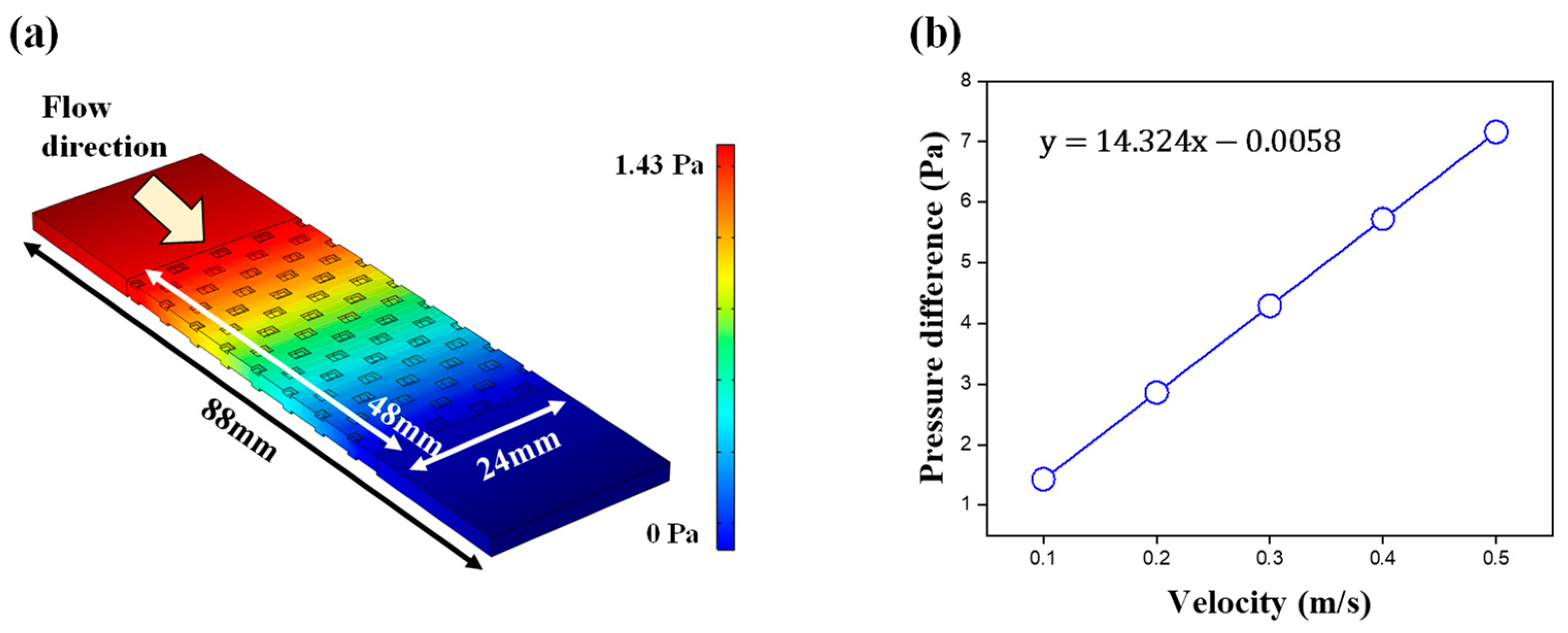
The corrugated plate is designed with a trapezoidal structure. This structure allows the gas to be uniformly distributed, thereby improving the fuel cell performance. In this study, the corrugated plate is assumed to be a porous medium. Therefore, the permeability of the corrugated plate was calculated based on the actual geometry using a fluid simulation. In the fluid simulation, the corrugated plate was designed to have a width of 24 mm, a length of 88 mm, and height of 2.4 mm, as shown in Figure 5a. Open structures were used for the inlet and outlet to achieve uniform gas movement.

The permeability (α) of the corrugated plate was obtained using Darcy’s law, as shown in Equation (34) [15]. First, the relationship of the pressure difference (ΔP) according to the gas flow rate was calculated through the fluid simulation. Furthermore, the permeability was determined using the viscosity coefficient (μ) and the distance of the gas (L). The permeability of the corrugated plate was derived as 8.15 × 10⁻⁸. Figure 5b shows the results of the pressure difference according to velocity.

$$\Delta P=-\frac{\mu ·L}{\alpha }{\displaystyle \sum }_{i=1}^n{v}_i$$

(34)

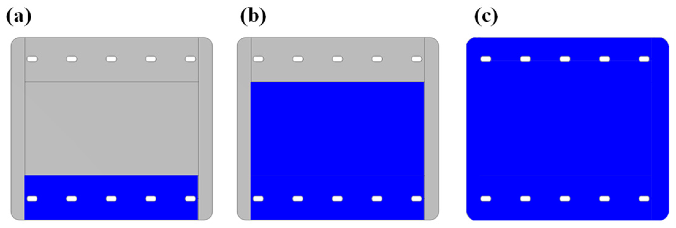
In this study, COMSOL Multiphysics 6.0 was used to compare the performance of external reforming and internal reforming-type MCFCs. The basic operating conditions are listed in

Table 1. Basic operating conditions of MCFCs.

Activation Area (cm)	Target Current Density (mA/cm2)	Flow Direction	S/C Ratio	Gas Utilization (%)	Operating Temperature (°C)	Reforming Area
647.5	150	Co-flow	3	40	620	Entire

. Based on the basic conditions, simulations were conducted according to the operating temperature, flow direction, and gas utilization in external reforming-type MCFCs. During internal reforming, the simulation was performed using the S/C ratio and reforming area as variables.

Table 2. Operating conditions in (a) external and (b) internal reforming-type MCFCs.

(a) External Reforming-Type MCFCs
Operating temperature (°C)	580	620		650
Flow direction	Co-flow		Counter-flow
Gas utilization (%)	20	40		60
(b) Internal Reforming-Type MCFCs
S/C ratio	2	3		4
Reforming area	A	B		C (Entire)

shows the operating conditions of the external and internal reforming-type MCFCs, and Figure 6 shows a schematic of the reforming area.

Table 3. Flow rate of inlet in the operating conditions of external reforming-type MCFCs.

Flow Direction	Operating Temperature (°C)	Gas Utilization (%)	Flow Rate of Inlet Gas
			Anode Side (m3/s)	Cathode Side (m3/s)
Co-flow	580	20	2.5601 × 10−4	6.2695 × 10−4
Co-flow	580	40	1.2227 × 10−4	2.9944 × 10−4
Co-flow	580	60	8.5335 × 10−5	2.0898 × 10−4
Co-flow	620	40	1.2800 × 10−4	3.1349 × 10−4
Co-flow	650	40	1.3230 × 10−4	3.2401 × 10−4
Counter-flow	580	40	1.2227 × 10−4	2.9944 × 10−4

and

Table 4. Flow rate of inlet in the operating conditions of internal reforming-type MCFCs.

Flow Direction	Operating Temperature (°C)	Gas Utilization (%)	S/C Ratio	Reforming Area	Flow Rate of Inlet Gas
					Anode Side (m3/s)	Cathode Side (m3/s)
Co-flow	580	20	2	C	1.3060 × 10−4	3.1348 × 10−4
Co-flow	580	40	3	C	1.4191 × 10−4	3.1348 × 10−4
Co-flow	580	60	4	C	1.5641 × 10−4	3.1348 × 10−4
Co-flow	620	40	3	A	1.4191 × 10−4	3.1348 × 10−4
Co-flow	650	40	3	B	1.4191 × 10−4	3.1348 × 10−4

are the flow rate of inlet gas according to the operating conditions in the external and internal reforming-type MCFCs. Meanwhile, the boundary condition of the outlet is atmospheric pressure without back flow, and the boundary condition of the wall is the no slip condition.

3. Simulation Results

3.1. External Reforming-Type MCFCs

3.1.1. Simulation Results according to Flow Direction

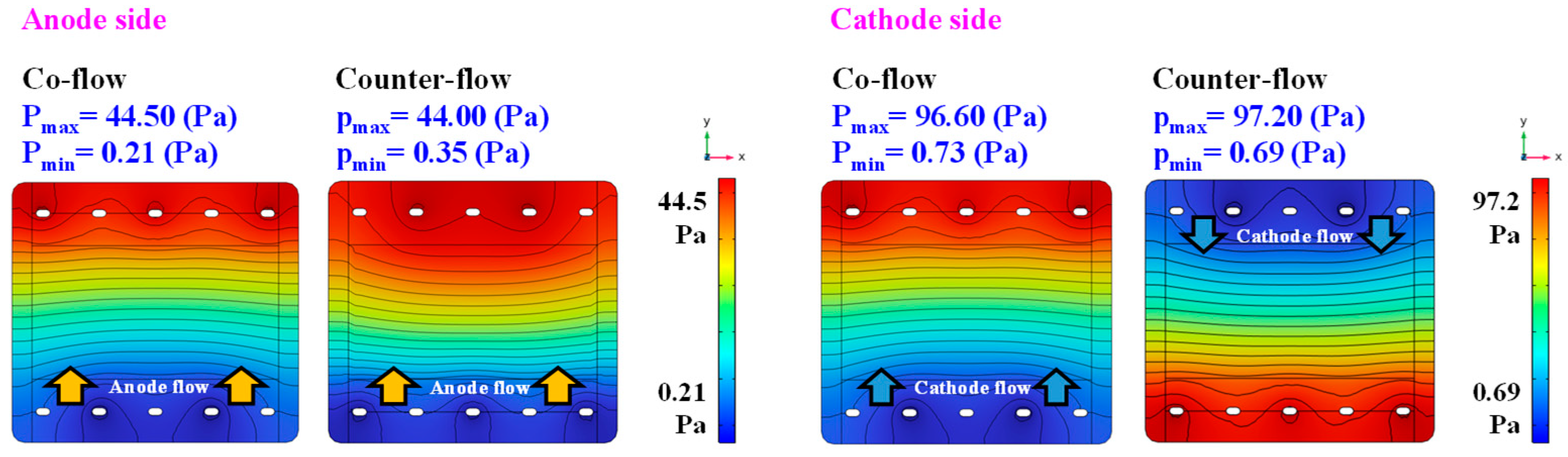
Figure 7 shows the results of pressure distribution according to the flow direction. The pressure differences between the co-flow and counter flows were compared. All the other conditions were identical. As a result, the pressure difference was 95.84 Pa in co-flow and 96.51 Pa in counter-flow at the cathode. The pressure differences were similar, depending on the flow direction at the anode and cathode.

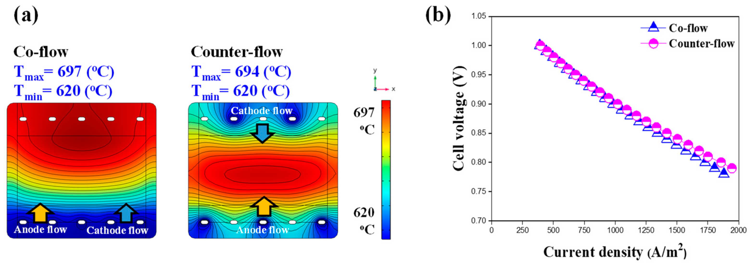
Figure 8a shows the result of the temperature distribution according to the flow direction. In the co-flow, the maximum temperature was concentrated at the outlet. This is because the heat generated in the fuel cell owing to the electrochemical reaction moves toward the outlet along the flow direction. However, gas was injected from both sides of the fuel cell, and heat was not exhausted in the counter flow. Therefore, the maximum temperature was concentrated at the center of the fuel cell. The temperature difference between the inlet and outlet was similar at 77 °C in co-flow and 74 °C in counter-flow.

Figure 8b presents a performance comparison according to the flow direction. The cell voltage was 0.83 V at the 1500 A/m² in co-flow. Furthermore, the cell voltage was 0.84 V at the 1500 A/m² in counter-flow. Therefore, the performance was slightly superior in counter flow compared to that in co-flow.

3.1.2. Simulation Results with Different Gas Utilizations

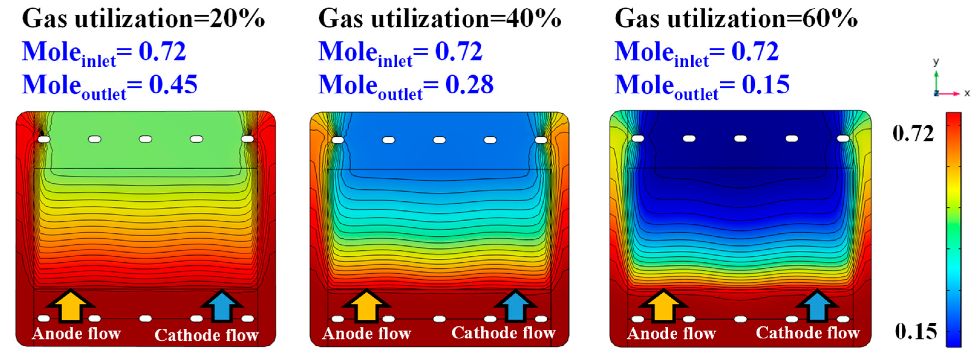
Figure 9 shows the concentration distribution of hydrogen according to gas utilization. The hydrogen concentrations at the outlet were 45%, 28%, and 15% for gas utilization rates of 20%, 40%, and 60%, respectively. This is because, as the gas utilization decreases, more hydrogen is injected into the fuel cell. Thus, a relatively large amount of hydrogen remained at the outlet.

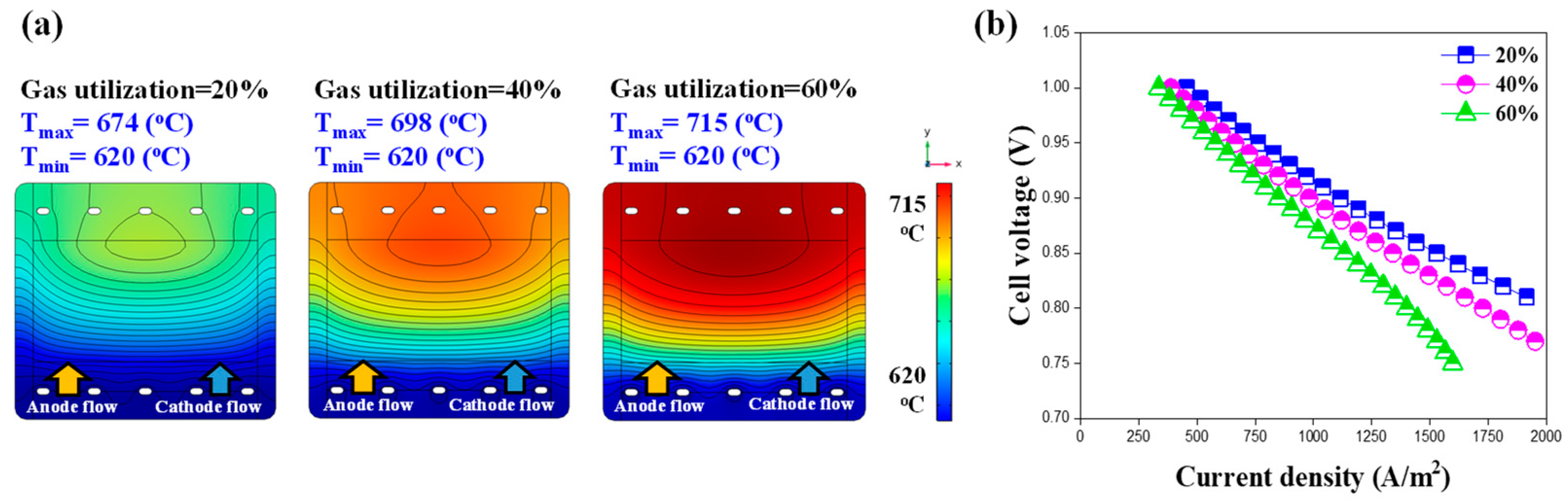
As shown in Figure 10a, the maximum temperatures were 674 °C, 698 °C, and 715 °C according to the 20%, 40%, and 60% gas utilization. This is because when the gas utilization rate is lowered, the amount of unreacted oxygen increases. Therefore, the temperature of the fuel cell decreased.

Figure 10b shows the performance according to gas utilization. The cell voltages were 0.85 V, 0.83 V, and 0.78 V at 1500 A/m², according to 20%, 40%, and 60% gas utilization. In this study, the flow rate of gas injected into the fuel cell was determined by Equation (9). Therefore, because of the lower gas utilization, more fuel was injected, and the performance improved.

3.1.3. Simulation Results with Different Operating Temperatures

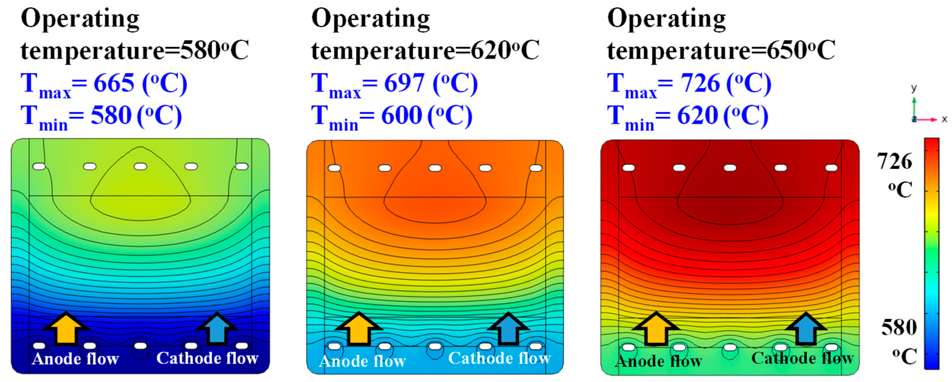
Figure 11 shows the temperature distribution with respect to the operating temperature. The maximum temperatures were 665 °C, 697 °C, and 726 °C at operating temperatures of 580 °C, 620 °C, and 650 °C. Furthermore, the temperature differences between the maximum and minimum temperatures were 82 °C, 97 °C, and 106 °C. Therefore, not only the maximum temperature, but also the temperature difference increased as the operating temperature increased.

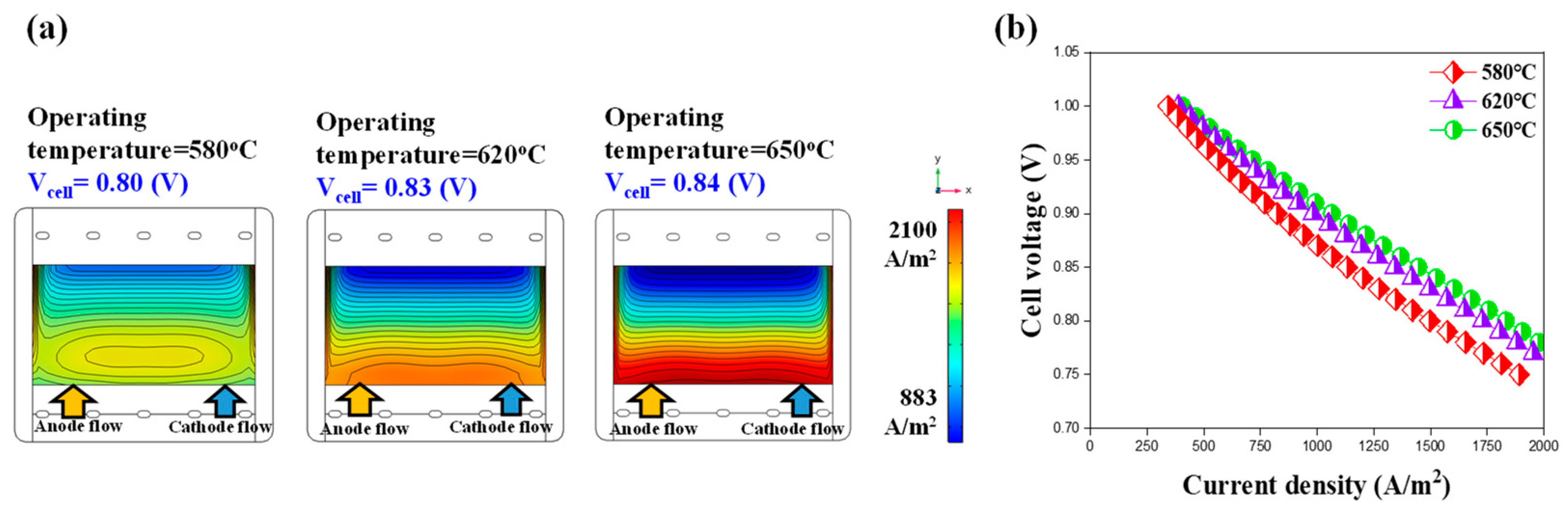
The current density distribution and performance, according to the operating temperature, are shown in Figure 12a,b, respectively. The cell voltages were 0.80 V, 0.83 V, and 0.84 V at 1500 A/m², according to the operating temperature. In general, the voltage of a fuel cell is calculated by subtracting the resistance loss from the Nernst potential, as shown in Equation (3). As the operating temperature increased, the performance improved because the rate of the decrease in resistance loss was higher than the rate of the decrease in the Nernst potential.

3.2. Internal Reforming-Type MCFCs

3.2.1. Simulation Results according to S/C Ratio

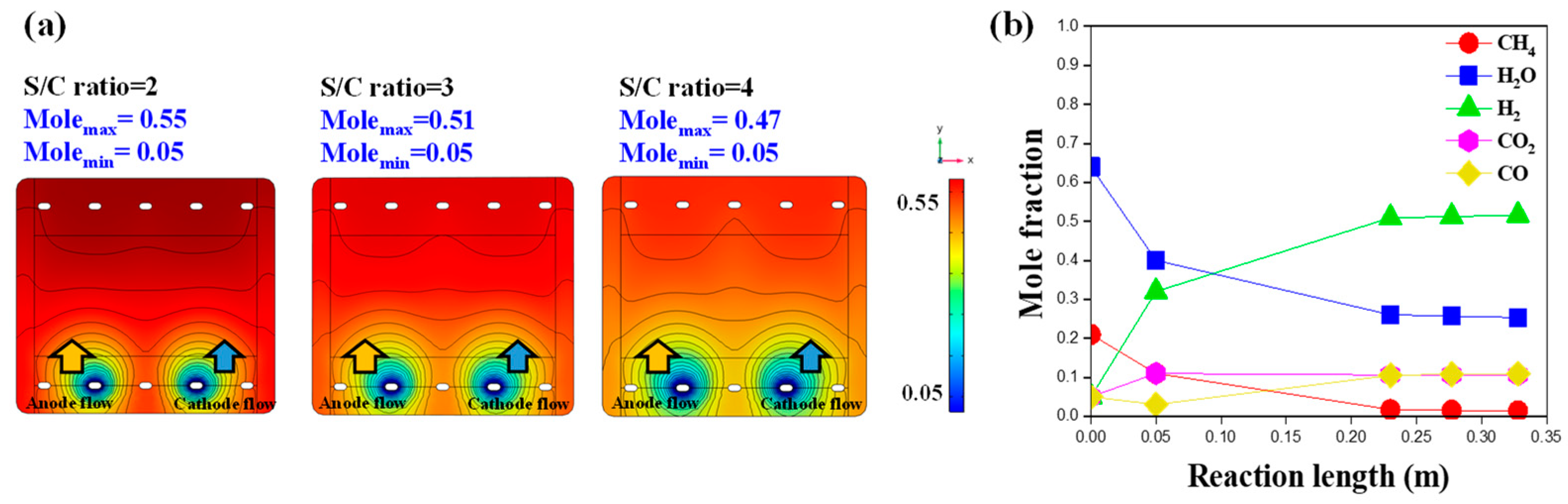
Figure 13a shows the distribution of hydrogen concentration, according to the S/C ratio. In addition, electrochemical reactions were not considered when comparing the reforming reactions, according to the S/C ratio in this simulation. When the S/C ratios were 2, 3, and 4, the hydrogen concentrations were 55%, 51%, and 47%, respectively. More hydrogen is produced as the S/C ratio decreases. This is because the lower the S/C ratio, the more hydrogen is produced because the concentrations of methane and steam become similar, and relatively more reforming reactions are generated.

Figure 13b shows the change in the concentration according to the chemical composition at an S/C ratio of 3. Steam and methane rapidly decrease, and hydrogen increases because of the reforming reaction at the inlet. In addition, the amounts of carbon monoxide and carbon dioxide increase slightly after the reforming reaction.

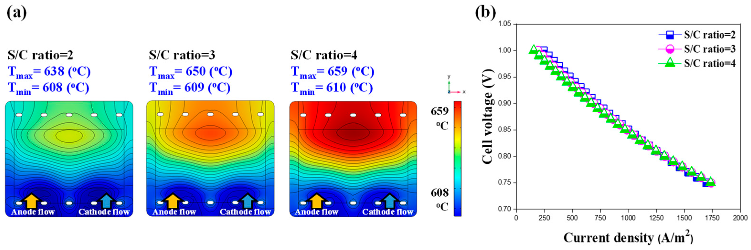
Figure 14a shows the temperature distribution according to the S/C ratio, considering the electrochemical reaction. Under all conditions, the minimum temperature occurred at the inlet owing to an endothermic reaction generated by the reforming reaction. The maximum temperature occurred at the outlet owing to the fluid characteristics of the co-flow. The average temperatures were 624 °C, 631 °C, and 637 °C, according to the S/C ratios of 2, 3, and 4. In addition, the fuel cell operated close to the operating temperature because the strongest endothermic reaction occurred at an S/C ratio of 2. Therefore, they are unsuitable for long-term fuel cell operations. Figure 14b shows the performance as a function of the S/C ratio. The cell voltages were 0.77 V, 0.78 V, and 0.78 V at the current density of 1500 A/m², according to the S/C ratios of 2, 3, and 4, respectively. Similar cell voltages were obtained for all S/C ratios.

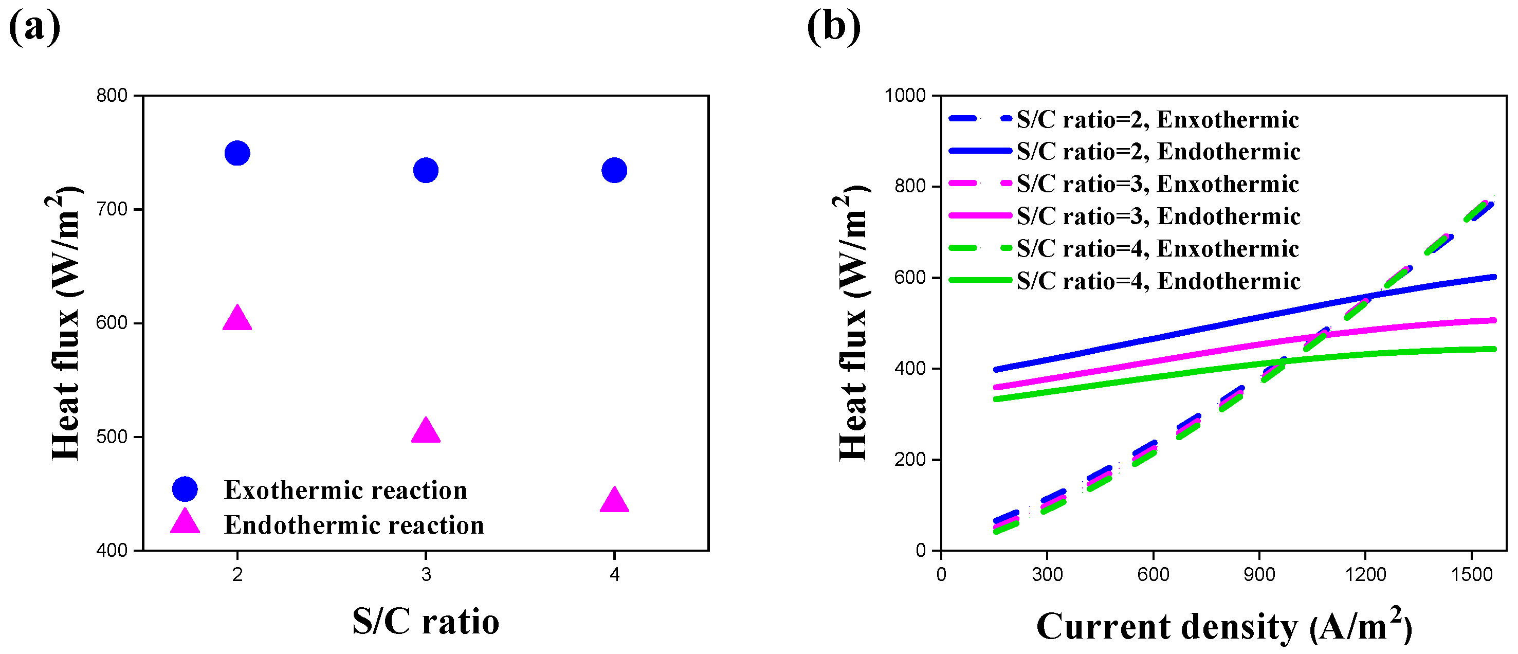
Figure 15a compares the heat fluxes of the exothermic and endothermic reactions according to the S/C ratio at 1500 A/m². Macroscopically, an exothermic reaction is generated by an electrochemical reaction, and an endothermic reaction is generated by the reforming reaction. The heat fluxes of the endothermic reaction were 602 W/m², 504 W/m², and 442 W/m² according to the S/C ratios of 2, 3, and 4, respectively. The largest endothermic reaction was observed at an S/C ratio of 2, where the reforming reaction generated the most energy. In contrast, the heat fluxes of the exothermic reaction were 750 W/m², 734 W/m², and 734 W/m², which were similarly generated.

Figure 15b compares the heat fluxes of the exothermic and endothermic reactions with respect to the current density. According to the S/C ratio, the difference in the heat flux of the endothermic reaction is greater than the difference in the heat flux of the exothermic reaction. In addition, the intersection heat fluxes of the endothermic and exothermic reaction were 1245 W/m², 1102 W/m², and 968 W/m² at S/C ratios of 2, 3, and 4, respectively. This intersection point corresponded to the thermally neutral point. The target current density of the fuel cell should exceed this threshold.

3.2.2. Simulation Results with Different Reforming Regions

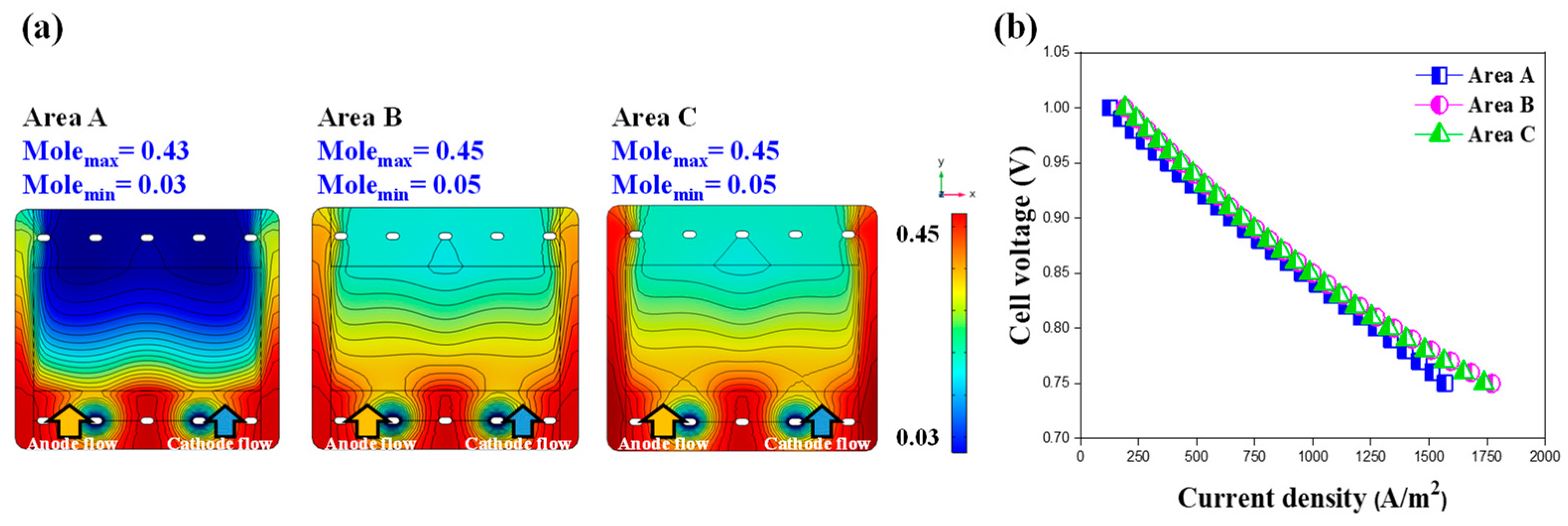
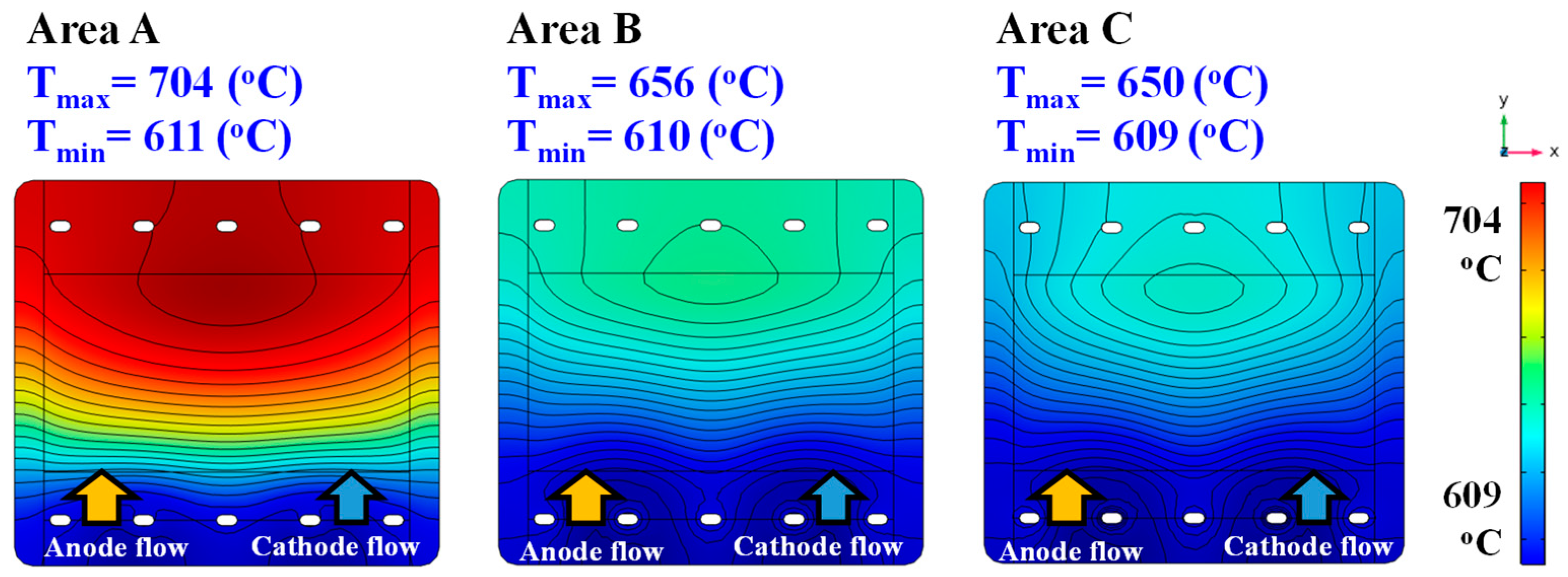
Figure 16a shows the hydrogen distribution based on the reforming area. The maximum hydrogen concentrations are 4 3%, 45%, and 45% in areas A, B, and C, respectively. Area A produced the lowest amount of hydrogen.

Figure 16b shows the performance according to the reforming area. Since the least hydrogen was produced in region A, the smallest cell voltage was accordingly 0.76 V at 1500 A/m². Furthermore, the same cell voltage was 0.78 V at 1500 A/m² in areas B and C. In the outer area of the fuel cell, more hydrogen was produced in area C. However, the same hydrogen concentration distribution was generated in areas B and C at 41% of the active area. Therefore, the same cell voltage was used as the output.

Figure 17 shows the temperature distribution according to the reforming area. The temperature difference between the maximum and minimum temperatures was 93 °C, 46 °C, and 41 °C in areas A, B, and C, respectively. Thus, the temperature difference was the smallest in area C. This is because, as the reforming area increases, more reforming reactions are generated, and the temperature decreases owing to endothermic reactions.

3.3. Comparison of Internal and External Reforming-Type MCFCs

In this study, the characteristics of internal and external reforming type MCFCs were compared under the basic operating conditions shown in Table 1 to analyze the characteristics of MCFCs, according to the type of reforming.

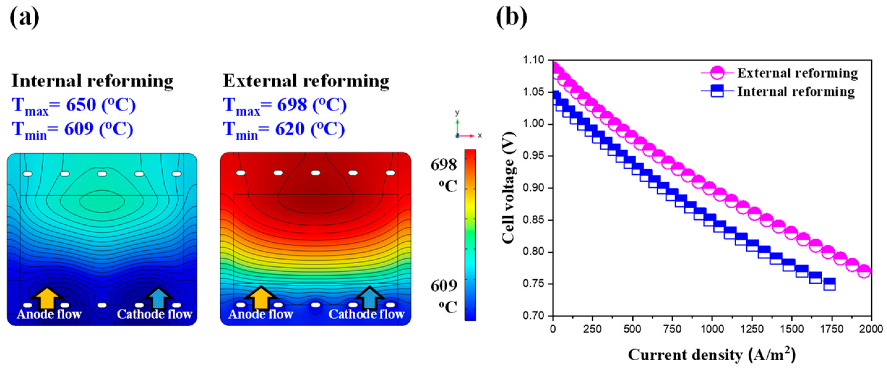
Figure 18a shows the temperature distributions in the internal and external reforming-type MCFCs. The temperature difference between the maximum and minimum was 41 °C in the internal reforming-type MCFCs and 78 °C in the external reforming-type MCFCs. Therefore, compared to external reforming-type MCFCs, internal reforming-type MCFCs can efficiently manage heat during fuel cell operation.

Figure 18b shows a comparison of the performance of the internal and external reforming-type MCFCs. The cell voltage of the external reforming-type MCFCs was 0.83 V at 1500 A/m². The cell voltage of the internal reforming-type MCFCs was 0.78 V at 1500 A/m². Thus, the performance of the external reforming-type MCFCs was better than that of the internal reforming-type MCFCs. This was because the hydrogen concentration of the fuel was fixed at 72% in the external reforming-type MCFCs. However, in the internal reforming-type MCFC with an S/C ratio of 3, 51% hydrogen was produced. Therefore, more hydrogen was injected into the external reforming-type MCFCs, and this is the reason why the performance of the external reforming-type MCFCs was superior to that of the internal reforming-type MCFCs.

$${\epsilon }_{real}={\epsilon }_{ideal}\times {\epsilon }_{voltage}\times {\epsilon }_{fuel}=\left(\frac{\Delta \widehat{g}}{\Delta {\widehat{h}}_{HHV}}\right)\times \left(\frac{V}{E_{OCV}}\right)\times \left(\frac{v_{used}}{v_{total}}\right)$$

(35)

In addition, the real efficiencies of the external and internal reforming-type MCFCs were compared. The real efficiency of a fuel cell (${\epsilon }_{real}$) can be calculated as shown in Equation (35), using the ideal efficiency, voltage efficiency, and fuel efficiency, where the higher heating value (Δh_HHV) used to calculate the ideal efficiency was −286 KJ/mol [16]. Thus, the real efficiencies of the external and the internal reforming-type MCFCs were 20.81% and 20.63%, respectively. The efficiency of the fuel cell was similar in the external reforming-type MCFCs than in the internal reforming-type MCFCs.

4. Conclusions

In this study, the electrochemical reaction, fluid, heat transfer, and reforming reaction of the external and internal reforming-type molten carbonate fuel cells were simulated using CFD. Furthermore, the characteristics of MCFCs according to the various operating conditions were compared in the same internal manifold.

The flow direction, gas utilization, and operating temperature were compared in the external reforming-type MCFCs. Similar pressure drops occur, according to the flow direction, but there is a difference in temperature distribution. At the gas utilization of 20%, 40% and 60%, the cell voltage decreased by 2.35% and 8.23%, based on the gas utilization of 20%. As the gas utilization decreases, more power can be produced because more hydrogen and air are injected into the same reaction area. At operating temperatures of 580 °C, 620 °C, and 650 °C, the cell voltage increased by 3.75% and 5%, based on the operating temperature of 580 °C. However, a suitable operating temperature must be determined by considering the mechanical and thermal properties of the fuel cell.

The S/C ratio and modified area were compared in the internal reforming-type MCFCs. Hydrogen produced in the S/C ratio of 2, 3, and 4 decreased by 7.27% and 14.54%, based on the S/C ratio of 2. Moreover, long-term operation is relatively difficult because it functions near the operating temperature when the S/C ratio is 2. Among the reforming areas of A, B, and C, the best performance was derived in the reforming areas of B and C, including the active area. Therefore, a difference in performance is generated, depending on whether the active area is included in the fuel cell.

The external and internal reforming-type MCFCs were compared. The temperature generated in the external reforming-type MCFCs is higher than that in the internal reforming-type MCFCs. The reason is that an endothermic reaction occurs in the internal reforming-type MCFCs. In addition, the performance of the external reforming-type MCFCs was superior to the performance of the internal reforming-type MCFCs. However, internal reforming-type MCFCs are effective in terms of heat management.

Meanwhile, differences in the quantitative values of simulations may occur, depending on differences in the reference data. However, since it takes time and money to compare experimental results under various conditions, it is valuable as a comparison of macroscopic results through simulation. Therefore, this study is expected to be efficiently utilized for the simulation of the design and operating conditions of MCFCs.

References

- Sharaf, O.S.; Orhan, M.F. An overview of fuel cell technology: Fundamentals and applications. Renew. Sustain. Energy Rev. 2014, 32, 810–853. [Google Scholar] [CrossRef]
- Lee, S.-J.; Lim, C.-Y.; Lee, C.-W. Design of Cell Frame Structure of Unit Cell for Molten Carbonate Fuel Cell Using CFD Analysis. Trans. Korean Hydrogen New Energy Soc. 2018, 29, 56–63. [Google Scholar] [CrossRef]
- Yu, J.-H.; Lee, C.-W. Effect of Cell Size on the Performance and Temperature Distribution of Molten Carbonate Fuel Cells. Energies 2020, 13, 1361. [Google Scholar] [CrossRef] [Green Version]
- Kim, Y.-J.; Lee, M.-C. Comparison of thermal performances of external and internal reforming molten carbonate fuel cells using numerical analyses. Int. J. Hydrogen Energy 2017, 42, 3510–3520. [Google Scholar] [CrossRef]
- Kim, Y.-J.; Chang, I.-G.; Lee, T.-W.; Chung, M.-K. Effects of relative gas flow direction in the anode and cathode on the performance characteristics of a Molten Carbonate Fuel Cell. Fuel 2010, 89, 1019–1028. [Google Scholar] [CrossRef]
- Jung, K.-S.; Lee, C.-W. Performance Analysis in Direct Internal Reforming Type of Molten Carbonate Fuel Cell (DIR-MCFC) according to Operating Conditions. Trans. Korean Hydrogen New Energy Soc. 2022, 33, 363–371. [Google Scholar] [CrossRef]
- Kim, H.-S. An Improved 3D Heat and Fluid Analysis for the MCFC Stack with Internal Manifolds. Master’s Thesis, KAIST, Deajeon, Republic of Koera, 2010. Available online: http://library.kaist.ac.kr (accessed on 29 December 2005).
- Zhao, C.; Yang, J.; Zhang, T.; Yan, D.; Pu, J.; Chi, B.; Li, J. Numerical simulation of flow distribution for external manifold design in solid oxide fuel cell stack. Int. J. Hydrogen Energy 2017, 42, 7003–7013. [Google Scholar] [CrossRef] [Green Version]
- Lee, C.-W.; Lee, M.; Yoon, S.-P.; Ham, H.-C.; Choi, S.-H.; Han, J.-h.; Nam, S.-W.; Yang, D.-Y. Study on the effect of current collector structures on the performance of MCFCs using three-dimensional fluid dynamics analysis. J. Ind. Eng. Chem. 2017, 51, 153–161. [Google Scholar] [CrossRef]
- Yuh, C.Y.; Selman, J.R. Polarization of the Molten Carbonate Fuel Cell Anode and Cathode. J. Electrochem. Soc. 1984, 131, 1984–2069. [Google Scholar] [CrossRef]
- Ramandi, M.Y.; Berg, P.; Dincer, I. Numerical analysis of transient processes in molten carbonate fuel cells via impedance perturbations. J. Power Sources 2013, 231, 134–145. [Google Scholar] [CrossRef]
- Pfafferodt, M.; Heidebrecht, P.; Sundmacher, K.; Würtenberger, U.; Bednarzs, M. Multiscale Simulation of the Indirect Internal Reforming Unit (IIR) in a Molten Carbonate Fuel Cell (MCFC). Ind. Eng. Chem. Res. 2008, 47, 4332–4341. [Google Scholar] [CrossRef]
- Freni, S.; Maggio, G.; Passalacqua, E. Modeling of porous membranes for molten carbonate fuel cells. Mater. Chem. Phys. 1997, 48, 199–206. [Google Scholar] [CrossRef]
- Lee, J.-S.; Seo, J.-h.; Kim, H.-Y.; Chung, J.-T.; Yoon, S.-S. Effects of combustion parameters on reforming performance of a steam–methane reformer. Fuel 2013, 111, 461–471. [Google Scholar] [CrossRef]
- Koh, J.-H.; Seo, H.-K.; Lee, C.-G.; Yoo, Y.-S.; Lim, H.-C. Pressure and flow distribution in internal gas manifolds of a fuel-cell stack. J. Power Sources 2003, 115, 54–65. [Google Scholar] [CrossRef]
- O’Hayre, R.; Cha, S.-W.; Colella, W.G.; Prinz, F.B. Fuel Cell Fundamentals, 3rd ed.; Wiley & Sons: New York, NY, USA, 2016; Chapter 2; pp. 62–64. [Google Scholar]
- Yaws, C.L. Heat capacity of gas. In Chemical Properties Handbook, 1st ed.; McGraw-Hill Education: New York, NY, USA, 1999; Chapter 2; pp. 30–55. [Google Scholar]
- Bird, R.; Stewart, W. Transport Phenomena, 2nd ed.; John Wiley & Sons: New York, NY, USA, 2002; Chapter 17; p. 521. [Google Scholar]
- Kong, W.; Gao, X.; Liu, S.; Su, S.; Chen, D. Optimization of the Interconnect Ribs for a Cathode-Supported Solid Oxide Fuel Cell. Energies 2014, 7, 295–313. [Google Scholar] [CrossRef] [Green Version]
- Yaws, C.L. Heat capacity of gas. In Thermal Conductivity of Gas, 1st ed.; McGraw-Hill Education: New York, NY, USA, 1999; Chapter 23; pp. 505–530. [Google Scholar]
- Xu, J.; Froment, G.F. Methane steam reforming, methanation and water-gas shift: I. Intrinsic kinetics. AIChE J. 1989, 35, 88–96. [Google Scholar] [CrossRef]
- Koh, J.-H.; Kang, B.-S.; Lim, H.-C. Analysis of temperature and pressure fields in molten carbonate fuel cell stacks. AIChE J. 2001, 47, 1941–1956. [Google Scholar] [CrossRef]
Figure 1.
Schematic of the molten carbonate fuel cells (MCFCs).
Figure 2.
Schematic diagram of the reaction surface in MCFCs.
Figure 3.
Schematic diagram of the internal manifold-type MCFCs.
Figure 4.
Schematic diagram of the internal manifold-type MCFCs for simulation.
Figure 5.
(a) Fluid simulation in corrugated plate and (b) pressure difference according to the velocity.
Figure 6.
Schematic of reforming areas (a) A, (b) B, and (c) C.
Figure 7.
Pressure distribution at the anode and cathode side, according to the flow direction.
Figure 8.
(a) Temperature distribution and (b) i–V curve, according to the flow direction.
Figure 9.
Hydrogen distribution according to the gas utilization.
Figure 10.
(a) Temperature distribution and (b) i–V curve, according to the gas utilization.
Figure 11.
Temperature distribution according to the operating temperature.
Figure 12.
(a) Current density distribution and (b) i–V curve, according to the operating temperature.
Figure 13.
(a) Hydrogen distribution according to the S/C ratio and (b) chemical composition at the S/C ratio of 3 in the absence of an electrochemical reaction.
Figure 14.
(a) Temperature distribution and (b) i–V curve according to the S/C ratio, considering the electrochemical reaction.
Figure 15.
Heat flux of the exothermic and endothermic reactions according to S/C ratios (a) at 1500 A/m2 and (b) the current density.
Figure 16.
(a) Hydrogen distribution and (b) i–V curve, according to the reforming area.
Figure 17.
Temperature distribution according to the reforming area.
Figure 18.
(a) Temperature distribution and (b) i–V curve under optimal conditions for external and internal reforming-type MCFCs.