Article

Influence of the Reward Function on the Selection of Reinforcement Learning Agents for Hybrid Electric Vehicles Real-Time Control

1
Interdepartmental Center for Automotive Research and Sustainable Mobility (CARS@PoliTO), Department of Energetics, Politecnico di Torino, Corso Duca degli Abruzzi 24, 10129 Turin, Italy
2
Department of Data Science, EURECOM, Route des Chappes 450, 06904 Biot, France
3
Addfor Industriale s.r.l., Piazza Solferino 7, 10121 Turin, Italy
*
Authors to whom correspondence should be addressed.
Submission received: 30 January 2023 / Revised: 25 February 2023 / Accepted: 10 March 2023 / Published: 15 March 2023
(This article belongs to the Special Issue Smart Energy Management for Electric and Hybrid Electric Vehicles)

Abstract

:
The real-time control optimization of electrified vehicles is one of the most demanding tasks to be faced in the innovation progress of low-emissions mobility. Intelligent energy management systems represent interesting solutions to solve complex control problems, such as the maximization of the fuel economy of hybrid electric vehicles. In the recent years, reinforcement-learning-based controllers have been shown to outperform well-established real-time strategies for specific applications. Nevertheless, the effects produced by variation in the reward function have not been thoroughly analyzed and the potential of the adoption of a given RL agent under different testing conditions is still to be assessed. In the present paper, the performance of different agents, i.e., Q-learning, deep Q-Network and double deep Q-Network, are investigated considering a full hybrid electric vehicle throughout multiple driving missions and introducing two distinct reward functions. The first function aims at guaranteeing a charge-sustaining policy whilst reducing the fuel consumption (FC) as much as possible; the second function in turn aims at minimizing the fuel consumption whilst ensuring an acceptable battery state of charge (SOC) by the end of the mission. The novelty brought by the results of this paper lies in the demonstration of a non-trivial incapability of DQN and DDQN to outperform traditional Q-learning when a SOC-oriented reward is considered. On the contrary, optimal fuel consumption reductions are attained by DQN and DDQN when more complex FC-oriented minimization is deployed. Such an important outcome is particularly evident when the RL agents are trained on regulatory driving cycles and tested on unknown real-world driving missions.

1. Introduction

Optimizing the energy management of an electrified vehicle under real-time conditions can be a demanding task. More specifically, the energy management system (EMS) of a hybrid electric vehicle (HEV) could require the solution of very complex optimization problems given that multiple power sources (thermal engine, motor-generators) and energy storage systems (batteries, ultra-capacitor) are embedded in the powertrain [1]. The assessment of the performance achieved by different strategies for on-board implementable EMSs is typically performed offline before moving to real-world driving cycles. Within such a framework, a virtual ecosystem must be developed to comprise a HEV model, a control strategy and a driving scenario [2]. Consistently, a simulation (or experiment) with type-approval driving cycles or real driving missions must be performed to investigate the response of the hybrid powertrain.
As far as real-time capable control strategies are concerned, a wide set of approaches has been developed in the recent years and proposed in the literature [3]. Among the latter, EMSs based on deterministic rules (RBC) [4] and the equivalent consumption minimization strategy (ECMS) [5] saw a major spread until 2010. Both RBC and ECMS hold the capability to achieve good results should a precise tuning operation be manually performed. More sophisticated techniques have hence been presented after 2010 to overcome such a major limitation, e.g., model predictive control (MPC) [6] and reinforcement learning (RL) [7]. Considering the impressive and continuous improvement in the research field of artificial intelligence (AI) [8], RL appears to be a very promising solution to design an intelligent control logic for HEV applications. Therefore, a detailed analysis of RL-based techniques for the energy management of HEVs is of major importance.
Several RL agents have been tested for HEV applications and various applications are to be found in the literature [9,10]. The performance of a Q-learning agent for a parallel HEV has been investigated in both [11,12]. The former considers the effects produced by a variation of some RL parameters; the latter focuses on the adaptability of Q-learning. In [13], Q-learning is adopted to optimize the fuel economy of a mild parallel HEV, outperforming both the baseline thermostatic rule-based EMS and ECMS. The results of the application of more sophisticated RL approaches to the real-time control of HEVs have also been presented in the literature. In [14], a deep Q-Network (DQN) was designed for a parallel hybrid architecture exploiting the learning actions of the state of the system. In [15], the authors successfully tested an online DQN algorithm to control the thermal engine and the continuously variable transmission of a parallel HEV. The application of DQN to a hybrid electric bus was also investigated in [16]. An evolution of DQN, namely double deep Q-Network (DDQN), was tested for a hybrid electric tracked vehicle and compared to a classic DQN in [17]. Other deep reinforcement learning (DRL) techniques have been presented (examples can be found in [18,19,20,21]) but are considered beyond the scope of the present article.
Regardless of the specific agent selected for a given test case, the literature of RL for HEV real-time EMS lacks a thorough assessment of the influence produced by different reward functions on the quality of the training process. In [11,12], one reward formulation was considered for the entire set of analyses with Q-learning agents. A similar operation was performed in [22] considering an enhanced variant of Q-learning. Moving to DRL, [16,17] account for fixed rewards even in the case of DQN and DDQN agents, respectively. Still, the response produced by such RL agents should be assessed as changes in the reward formulation are applied.
Different reward formulations could significantly alter the complexity of the control problem by increasing or decreasing the number of roadblocks in the training process. It is hence worth investigating the effects produced by different reward functions.
In the present paper, the assessment of the performance of four different agents is carried out considering two distinct reward functions. The latter was designed by drastically modifying the parameters of a single formulation to relevantly change the reward orientation. A detailed analysis of agent response was conducted considering both regulatory driving cycles and real-world driving missions as RL environments. In both cases, the focus was on the advantages brought by the specific selected agent. As a matter of fact, an increase in the complexity of the RL agent would not necessarily lead to improved performance.
The main contributions of the present paper can be summed up as follows.
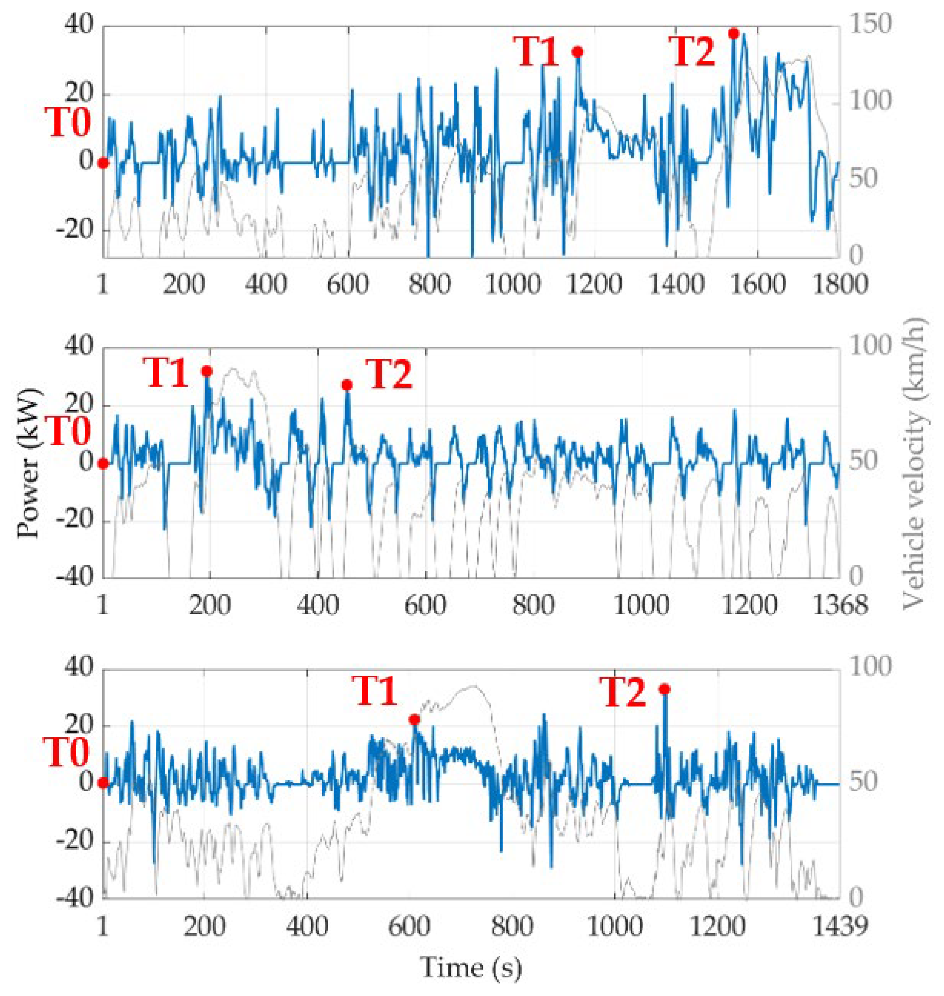
  • An approach to evaluate the meaningful stages of the driving missions for an appropriate assessment of the RL agent learning process;
  • An assessment of the change in the performances achieved by different RL agents trained on different regulatory driving cycles with two distinct reward functions;
  • A detailed analysis of the potential carried by the selected agent when tested on real-world driving conditions.
The article is organized as follows: the vehicle model and the general RL control framework are presented in Section 2, the main characteristics of a RL-based EMS for HEVs are presented in Section 3 and the main results of the analyses are discussed in Section 4.

2. Vehicle Model and Control Framework

Approaches based on RL require the definition of two main components, namely the agent and the environment, which are intended to interact continuously. In the research activity presented in this article, the agent–environment interactions were deployed through three different modules, namely the vehicle, the mission and the controller. The vehicle module comprises the HEV model and was used to predict the evolution of the system state (i.e., state dynamics) when a given control action was selected by the agent. The mission module constitutes the driving scenario and was modeled using the vehicle velocity signal tracked throughout the driving mission. Finally, the considered RL agents (Q-learning, DQN and DDQN) and the entire set of rules and parameters needed for the training process are embedded in the controller module. The integrated modular software framework (IMSF) presented in [23] was employed to connect the three models in a single virtual ecosystem and is not hereafter reported for the sake of conciseness.

2.1. Vehicle

In the vehicle module, a quasi-static backward-facing model of a pre-transmission parallel HEV architecture was developed [23] and used to simulate the evolution of the state of the system when a given control action was implemented by the agent module. This operation was replicated for each time step throughout the driving mission, i.e., at each stage of the training episode. Once the state evolved, the vehicle model sent a feedback signal to the environment module on the results of the training step that was accomplished.
According to the backward-facing modeling approach, the vehicle velocity profile of a given driving mission is considered as the exogenous input and translated into a reference power signal that must be satisfied by the powertrain. Starting from the power at the wheels, the power demand backwardly propagates to each driveline component (final drive, gearbox, torque-coupling device, clutches) up to the internal combustion engine (ICE) and the motor-generator (MG). As far as the main elements of the driveline are considered, speed ratios with fixed efficiencies were used to model the final drive, the torque-coupling device, and each gear of the transmission. Experimentally derived 2D look-up tables were employed for the fuel consumption and the efficiency of the ICE and the MG, respectively [23]. The battery was modeled as an equivalent resistant circuit [23]. Finally, the general specs of the vehicle used for the experiments as well as the main characteristics of the ICE, the MG and the battery are reported in Table 1.

2.2. Environment

The environment module sent an amount of meaningful information to the agent module at the end of each training step. Specifically, information about both the external world (i.e., the driving mission) and the updated state of the system was passed to the agent module to allow the latter to select new control actions.
Three different driving scenarios were considered for the analyses, i.e., the World Harmonized Light-Duty Test Cycle (WLTC) [24], the first two parts of the Federal Test Procedure (FTP-75) [25] and an experimentally derived real-world driving mission (RDM) [26]. The type-approval test cycles (WLTC and FTP-75) were considered to assess the capability of the RL-based agent to comply with the regulatory framework. On the contrary, RDM was selected to test the performances of the RL agents in a more realistic driving scenario. In Figure 1, the power profiles of the HEV for each driving scenario are charted along with the velocity trajectories. Note that the maximum and minimum power demands are comparable throughout the missions (≈40 kW in traction and ≈20 kW in braking) even if different distributions can be detected. On each power profile of Figure 1, the three marked time-steps assume a fundamental role for a detailed analysis of the RL agents performances. Specifically, T0 is the initial time step of the driving missions, whereas T1 and T2 are the stages of the missions with the maximum power requests. These two were defined as “attractors” given that the complexity of the control problem tends to increase as the training episode approaches them. In fact, the identification of the optimal chain of actions becomes a harder task given that a shrunken set of actions is feasible for such steps of the mission. Therefore, a smaller number of control sequences should be implemented in the time steps preceding the attractor so as to avoid unfeasibility. The attractors were hence considered to assess the effectiveness of the learning progress throughout the training phase.

2.3. Agent

At each stage of a training episode, the agent was responsible for selecting the control actions. The control problem was modeled through a Markovian decision process (MDP) [27] in which the environment cannot provide the agent with the entire information on the state of the system. Therefore, the signals transferred from the environment to the agent were considered as a subset of the state, namely the “observations”. The formulation of the control problem turned into a partially observable Markov decision process (POMDP) [28], where the observation satisfies the Markovian property.
The objective of any RL agent is that of maximizing the sum of the rewards obtained throughout the experiment. Given the necessity of avoiding a distinction between episodic and continuous tasks, the authors considered the unique notation of the discounted return G t , presented in [29]:
G t = k = t + 1 T γ k t 1 R k
where γ = [0, 1] is the discount factor, R k is the immediate reward and T is the final time-step. The latter can be set to infinite in case of γ < 1. Moreover, RL agents estimating the optimal action-value functions were considered, and the expected return was consistently evaluated as:
Q s , a = E π G t = E π k = t + 1 T γ k t 1 R k
where E π represents the expected value of the discounted return following a given policy π . Assuming the expectation of the value was met, the agent could choose the optimal action for every encountered state (or observation) by properly selecting the action corresponding to the largest value of Q s , a . Thanks to an efficient training process, the agent could achieve proper estimations of the Q-values.
A brief dissertation of the considered RL agents is reported hereafter. The first considered RL category was traditional Q-learning [30], in which observations and actions are discretized and the Q-values are stored in a matrix, namely the Q-table. At each time step t , the estimated new Q-values Q n related to a given tuple of observations O t and actions A t are updated using the old Q-values Q o through:
Q n O t , A t = Q o O t , A t + α U t
U t = R t + γ max a Q o O t + 1 , a Q o O t , A t
where α is the learning rate and U t is the updated Q-value. Q-learning achieves good performance in different applications despite its limitations. On the one hand, the discretization of the observation and the action impairs the possibility to apply and test all the possible control solutions. On the other hand, enlarging the Q-table (i.e., adding discretization levels), thus increasing the number of possible control solutions, leads to an increase in computational time (“curse of dimensionality”) as well as a worsening of the convergence to the optimal policy.
Beyond Q-learning, DRL algorithms have evidenced capability to deal with dimensionality issues by employing deep neural networks (DNNs). These are used as approximators to estimate action-value functions. Two DRL algorithms were hence considered in the present research paper, namely the DQN and the DDQN. In the DQN [31], a DNN, namely the “Q-network”, receives a continuous signal from the system state at each stage of the training episode. No discretization is needed, and the curse of dimensionality is mitigated given that any continuous change in the system state directly reflects in a change in the corresponding Q-value. High-dimensional state spaces can be hence handled without significantly compromising the computational time. Besides Q-networks, the DNN “target network” was introduced to guarantee algorithm stability. The weights of the target networks are updated every n step ( n > 1), with a lower frequency with respect to the Q-network [32]. Finally, the “experience replay memory” buffer was used to store the data needed to update the weights of the DNNs during the training operations. The full DQN and DDQN algorithms are presented in Algorithm 1.
The weights of the Q N network were randomly initialized before starting the training phase. At each time step t , the experience replay memory stored a tuple ( O t ,   A t ,   R t , O t + 1 ) containing the current observation O t , the current selected action A t , the immediate reward R t and the following observation O t + 1 . For every training iteration, a batch of random tuples (“mini-batch”) was sampled from the experience replay memory and used to train the Q-network. Consistent with the POMDP approach discussed for Q-learning, the state of the system was approximated by its observations. The formulation of the loss function of the Q-network can be written as:
L = R t + γ max a Q T O t + 1 , a Q N O t , A t
where Q T and Q N are the Q-values estimated by the target network and the Q-network, respectively. However, the DQN algorithm suffers from a possibly critical problem typically referred to as the overestimation bias [33]. Therefore, DDQN has been introduced in the literature as a DQN variant with the aim of avoiding bias in the estimation of the Q-values [34]. For the DDQN algorithm considered in the present paper, the loss function formulation of Equation (5) was modified to:
L = R t + γ Q T O t + 1 , argmax a Q ( O t + 1 , a ) Q N O t , A t
Four different RL agents were hence developed within the agent module of the IMSF: the Q-learning 1 obs, the Q-learning 3 obs, the DQN and the DDQN. The difference between the Q-learning 1 obs and the Q-learning 3 obs is discussed in the following Section. The hyperparameters of the considered agents are summarized in Table 2.
Algorithm 1 DQN and DDQN
Initialize Q-network Q N and target network O T with random weights
  for each episode do
    for each environment step do
    Collect observation O t and select action A t
    Execute A t and collect next observation O t + 1 and reward R t
    Store tuple O t ,   A t ,   R t , O t + 1 in memory replay buffer
    Sample tuple O t ,   A t ,   R t , O t + 1 from memory buffer
    Compute loss function of the Q-network:
       L = R t + γ max a Q T O t + 1 , a Q N O t , A t for DQN
       L = R t + γ Q T O t + 1 , argmax a Q ( O t + 1 , a ) Q N O t , A t for DDQN
    Perform gradient descent to update Q N
    Every n steps the Q T is updated
  end for
end for

3. Reinforcement Learning for the Energy Management of Hybrid Powertrains

The configuration of an RL agent must be properly tuned for the specific learning task. The observation, the action and the reward function considered in this article were chosen to highlight the potentials of RL when embedded into a real-time capable EMS for HEVs. In case of HEVs based on the charge-sustaining mode [35], one of the most interesting results is the minimization of fuel consumption (FC) without a full battery charge depletion. It is anyhow also worth considering different metrics in the vehicle control, e.g., pure charge sustaining. Therefore, the configuration of the RL-based controllers tested is describable by the set of observations, actions, and reward function pushing the agent towards either FC-oriented or SOC-oriented training.

3.1. Observation

Three different signals were considered for the observation, namely the battery state of charge (SOC), the vehicle velocity, and the vehicle acceleration. For three out of the four RL agents (i.e., Q-learning 3 obs, DQN and DDQN), all the observation signals were employed. On the contrary, the battery SOC was exploited as a stand-alone observation for the Q-learning 1 obs. Such an additional configuration was studied to test the performance of Q-learning with a restrained set of observations, which could promisingly avoid the dimensionality issues of Q-learning. The discretization of the SOC consisted of 500 levels within the SOC window [0.55–0.65] [36], whereas 10 levels were used for the vehicle velocity and acceleration.

3.2. Action

A wide spectrum of control decisions is possible for an HEV given that different optimal solutions can be targeted. For the present study, the action signals identified comprise the power-split between the ICE and the MG together with the gear number. Considering the pre-transmission HEV architecture modeled in the vehicle section, the power-split between the propellers is a key indicator of the operating mode of the powertrain, Moreover, the gear number affects the working point of both the ICE and the MG. A filtering operation was carried out to speed up the training process. More specifically, the real-time evaluation of the action feasibility was carried out, e.g., a given power-split might not be realized with a given gear number. Therefore, at a generic time step the agent could only choose amongst physically possible actions (“feasibility condition”), these representing a sub-set of the whole action set.

3.3. Reward

The formulation of the reward function is crucial for every RL agent as it is deeply connected to the optimization targets. The following reward function was considered to study the response of the agent to changes in the reward orientation:
R = { a + b · m ˙ f + c · m ˙ f , e q                       i f   0.55 < S O C < 0.65 p                                                                   i f   S O C < 0.55   |   S O C > 0.65
where a (positive), b (negative) and c (negative) are tuning coefficients, p is a negative penalty obtained when the battery SOC oversteps the SOC window boundaries, m ˙ f is the actual fuel consumption and m ˙ f , e q is the equivalent fuel consumption corresponding to a SOC level below the reference value:
m ˙ f , e q = S O C S O C · E b H i η I C E 1  
where S O C is the reference battery SOC (imposed to be equal to the initial value), E b is the energy content of the battery, H i is the lower heating value of gasoline and η I C E is an average ICE efficiency conventionally set to 0.35 for the present investigation. The formulation of Equation (8) was derived from the procedures of the WLTC framework. The real cumulative FC at the end of the driving mission is hence expressed as:
M f , r = M f + M f , e q
where M f is the cumulative FC and M f c , e q is the additional fuel to be added whenever S O C < S O C .
Two different reward function orientations were studied. More specifically, the so-called “SOC-oriented” and the so-called “FC-oriented” reward functions were obtained by imposing b = c and b c in Equation (7), respectively. The coefficients b and c were selected after a massive testing campaign characterized by several experiments in the WLTC driving mission. The SOC-oriented reward should thrust the RL agent to comply with an almost perfect charge-sustaining mode whilst reducing the FC as much as possible. In such case, a limited battery recharge was accepted at the end of the mission and a final battery SOC value lower than the initial one would not be tolerated (i.e., the experiment would be considered as failed). As far as the FC-oriented reward is concerned, the RL agent faced the opposite control problem, i.e., the agents targeted the minimization of the fuel consumption whilst maintaining the battery SOC within reasonable sustaining operations.

4. Results

The results of the two different reward function orientations are hereafter presented. A comparison was initially carried out among the responses obtained by the four RL agents discussed in Section 2 employing the two reward function orientations described above (i.e., SOC-oriented and FC-oriented) and two driving scenarios (WLTC and FTP-75). The adaptability of the trained agents was hence assessed for testing the performance on a real-world driving mission (RDM).
As far as the exploration strategy is concerned, a linearly decreasing ε -greedy policy was selected to model the exploration decay throughout the experiment. The value of ε for the first training episode ( E 1 ) was set to 0.8 and a minimum value of 0.05 was achieved in episode 375. From such episode onwards, the value of ε was no longer modified to maintain a small but constant exploration rate for the residual interval of the experiment. The experiments were performed on a i7-1165G7 2.80 GHz laptop.

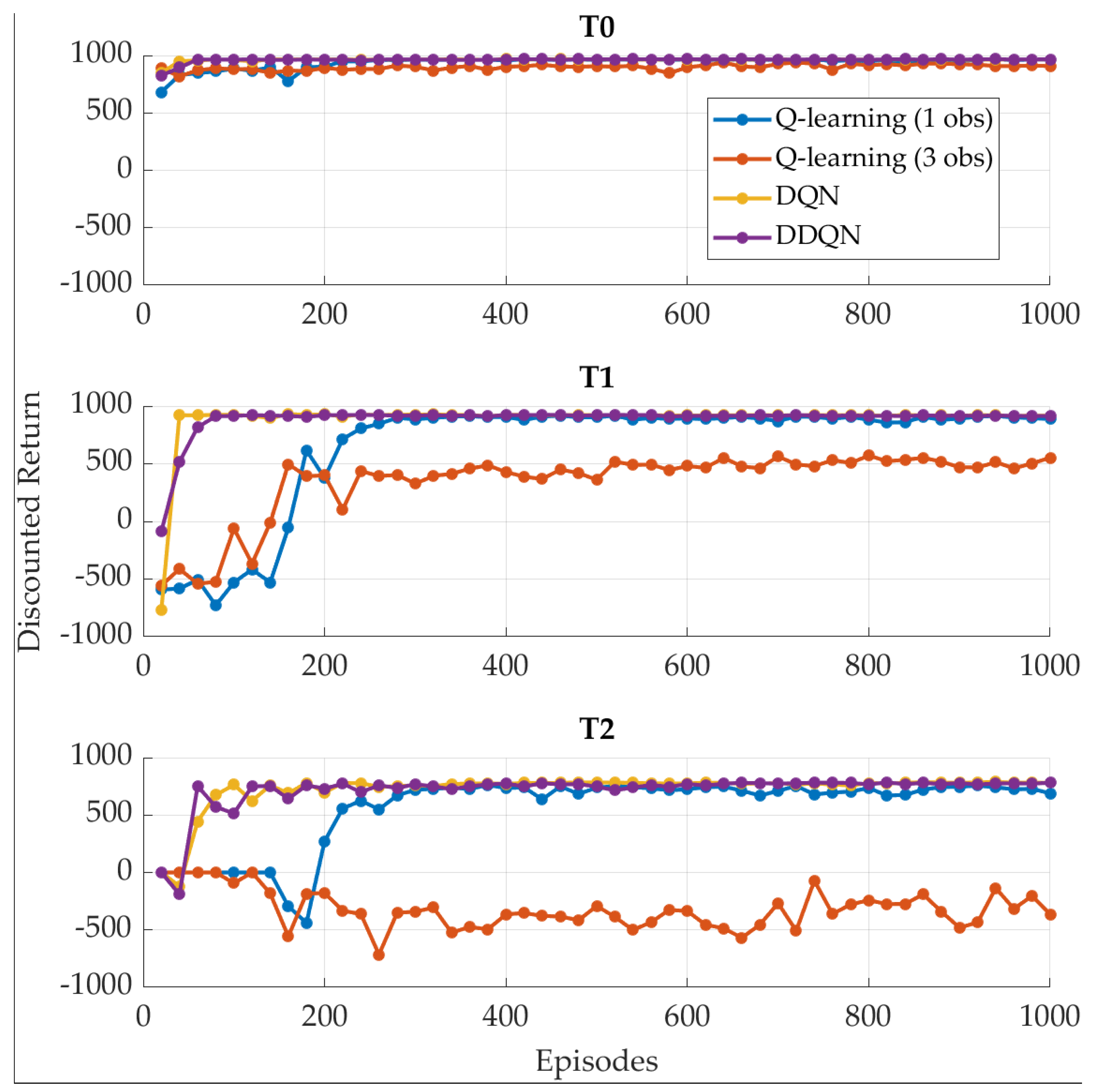
4.1. SOC-Oriented Reward

The effects produced by the variation in reward orientation on the performances of the Q-learning 1 obs, the Q-learning 3 obs, the DQN and the DDQN are presented in the present Section for the WLTC and FTP-75 type-approval cycles.
It is worth recalling that the SOC-oriented rewarding was designed to perfectly sustain the battery SOC, still complying with a minor recharge by the end of the mission. The SOC-oriented approach led to a simpler control problem given that the agent was merely forced to maintain the battery SOC close to its initial value, thus avoiding the battery SOC exceeding the limits of the SOC window. The battery SOC profiles produced by the policies of the considered RL agents at the end of the training process are reported in Figure 2 and Figure 3 for the WLTC and the FTP-75, respectively. For both missions, the battery SOC signals generated by the control policies of the Q-learning 1 obs (blue), the DQN (yellow) and the DDQN (purple) were consistent with the charge-sustaining task. In fact, the battery SOC was sustained for most of the driving cycles, whereas a relatively small recharge was only attained at the end of the episode. Furthermore, enlarging the observation of the Q-learning agent from 1 (Q-learning 1 obs) to 3 (Q-learning 3 obs) for a fixed number of training episodes (1000) did not improve the learning capability. Indeed, an overall battery discharge was produced by Q-learning 3 obs on both the WLTC and FTP-75. Such behavior can be ascribed to the increased number of tuples (observation-action) connected to the increased number of observations, thus enlarging the number of Q-values and hence impairing agent effectiveness.
In Table 3, four different metrics are reported to compare the numerical results obtained from the agents in terms of cumulative FC ( M f ), final battery SOC value ( S O C T ), and real cumulative FC ( M f , r ). The relative difference between the real fuel consumption of each agent with respect to the Q-learning 1 obs agent ( M f , r ) is also reported. Surprisingly, Q-learning 1 obs outperforms any other RL agent in terms of FC minimization on the WLTC. Interesting results are once more produced by the Q-learning 1 obs on the FTP-75, with a small increase in FC with respect to those produced by the other DRL agents.
The discounted return obtained at the end of each training episode over the two type-approval cycles is reported in Figure 4 and Figure 5 for a complete assessment of the performance of the training progress of the RL agents. More specifically, the discounted return evaluated in the initial time step of the missions (T0) and in the two attractors (T1 and T2) are reported in the upper, mid, and lower charts, respectively. It is worth underlining that null values were reported for the unfinished episodes.
The poor results reported in Table 3 for the Q-learning 3 obs are confirmed in Figure 4 and Figure 5 by the lowest discounted return trend. On the contrary, good trends are observed for the remaining RL agents. A difference can only be observed in the convergence rate as the DRL agents are faster than Q-learning 1 obs and the number of episodes needed for convergence increases from T0 to T2. Finally, the shape of the discounted return is investigated from a different perspective in Figure 6 and Figure 7. Specifically, the discounted return is plotted for the WLTC considering the actual mission time-steps for testing episode number 100 (Figure 6) and number 1000 (Figure 7), with pure exploitation. Consistent with the issues introduced by the attractors (see Section 2), the curves related to T1 and T2 bring significant information only when the attractors are properly overcome.
Such an unconventional representation of the discounted return allows for acknowledging the faster convergence to the final value of the DRL agents with respect to the Q-learning 1 obs. The training algorithm of the latter is, in fact, affected by an effective learning progress from episode 100 to episode 1000. As far as the SOC-oriented approach is concerned, the increased complexity of the RL agent is not counterbalanced by a refinement in the performance of the HEV control strategy.

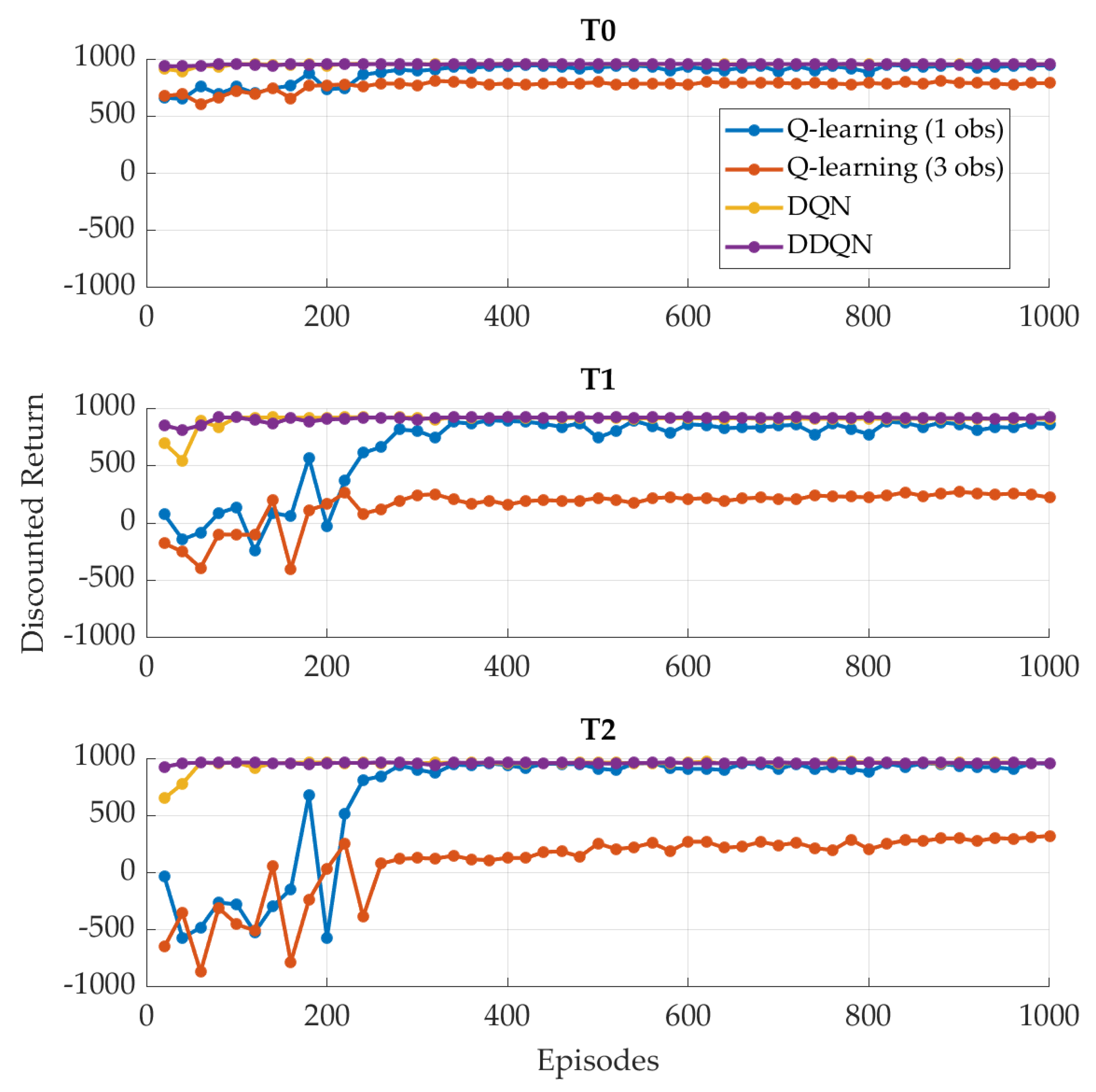
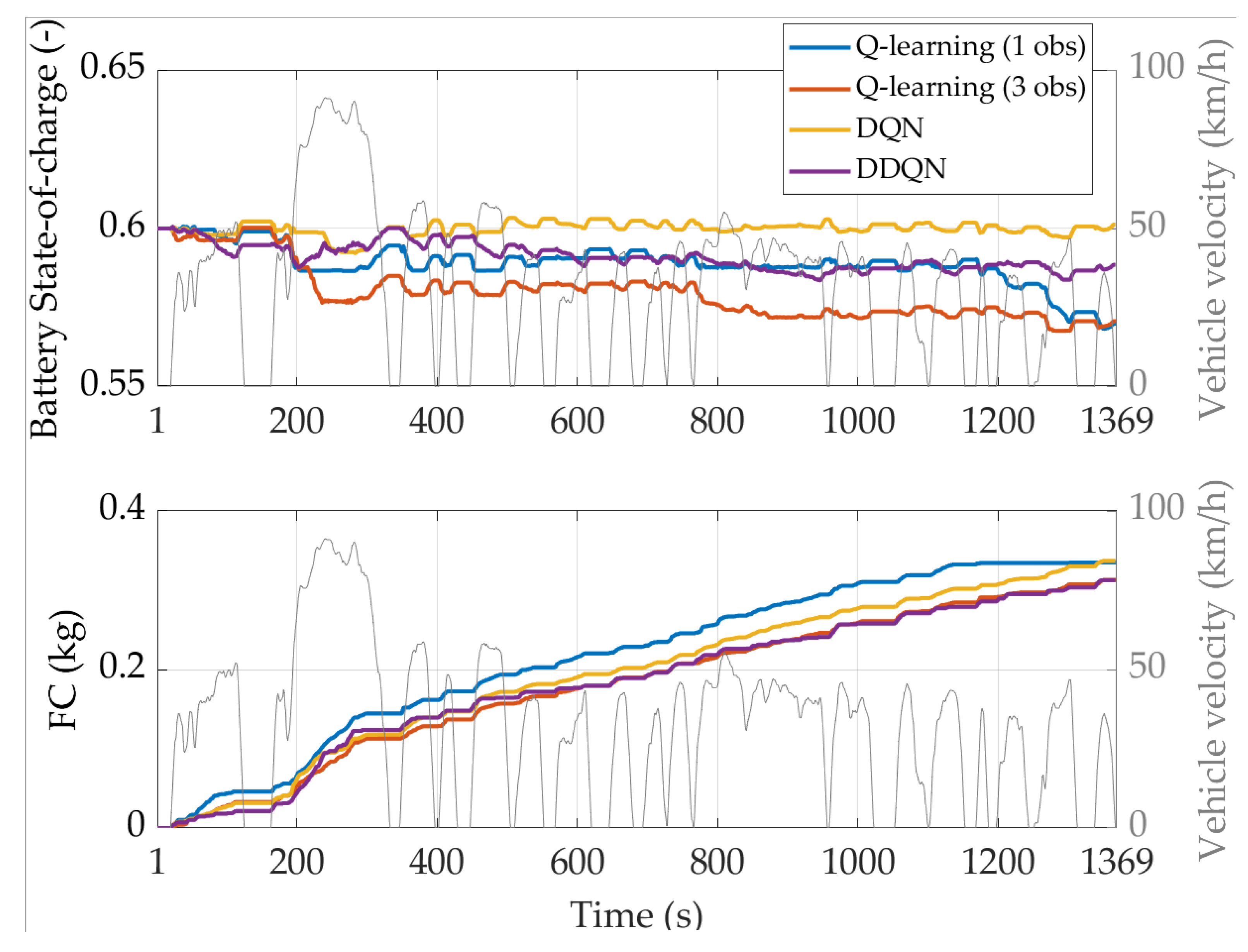
4.2. FC-Oriented Reward

The FC-oriented approach aims at minimizing the FC for the considered driving mission while constraining the battery SOC within its admissible SOC window. The trends of the battery SOC resulting from the last training episode are plotted along with the cumulative FC for the RL agents over the WLTC and the FTP-75 type-approval cycles in Figure 8 and Figure 9, respectively. The DRL-based controllers now significantly outperform the Q-learning ones. As far as the WLTC is concerned (Figure 8), the DQN (yellow) and the DDQN (purple) achieve the lowest final FC values. As a matter of fact, the Q-learning 1 obs is only able to sustain the battery SOC, whereas the Q-learning 3 obs fails to accomplish the task. The reasons behind such behavior are thoroughly explained in Section 4.1. As far as the FTP-75 scenario is concerned (Figure 9), DQN and DDQN still demonstrate superiority, whereas Q-learning 3 obs manages to complete the mission and promisingly outperform Q-learning 1 obs in terms of FC minimization. The increased performance of the Q-learning 3 obs is mainly ascribable to the shorter cycle duration and reduced power demand, thus reducing the complexity of the task. Nevertheless, although the Q-learning agents can achieve FCs comparable to the DQN and the DDQN, unsatisfactory battery SOC profiles are generated. The FTP-75 demonstrates that the RL agents holding a higher number of observations hold better performance. As a matter of fact, the FC is highly influenced by the vehicle speed and acceleration and hence better estimated when such information is fed to the agent. Still, the capability of the Q-learning 3 obs agent is strongly impaired for a more demanding and longer cycle such as the WLTC, where the high number of tuples (observation–action) cannot be fully explored. The DRL agents overcome this issue thanks to the continuous observation space.
In Table 4, the comparison among the real FCs is reported. It is worth noting that these results significantly differ from those related to the SOC-oriented reward (Table 3). The DQN and the DDQN agents achieve relevant FC savings compared to the Q-learning ones. Specifically, the DDQN produces the lowest FC for both the WLTC and the FTP-75 with a satisfactory battery charge-sustain.
The change in the reward configuration produces a modification to the learning curves as shown in Figure 10 (WLTC) and Figure 11 (FTP-75). Indeed, the discounted returns obtained throughout the whole training episodes for both WLTC and FTP-75 are not characterized by increasing trends when the initial time-step is considered (T0, upper charts). Instead, an increasing trend can be identified for the attractors T1 (mid charts) and T2 (lower charts), which is a clue to an effective training process. The analysis of the discounted return in the attractors T1 and T2 allows for a more appropriate assessment of the agent learning progress, which is not guaranteed by solely analyzing T0. Moreover, for the FC-oriented reward, the DRL-based agents better maximize the final value of the discounted return than Q-learning ones. Nevertheless, the convergence of the training process obtained with the FC-oriented reward for all the agents is slower than the one obtained with the SOC-oriented reward (Figure 4 and Figure 5). Such a result is due to the increased number of unfeasible episodes encountered by the agents. Indeed, the FC-orientation of the reward function pushes the agent to a wider utilization of the MG and hence to the exploration of low battery SOC regions. Thus, the agent can easily push the battery SOC out of the admitted SOC window (0.5–0.7) and generate an unfeasible condition that stops the training episode.
The trends of the discounted return evaluated for the WLTC scenario at testing episodes 100 and 1000 are reported in Figure 12 and Figure 13. The learning difficulties encountered by the agents are confirmed as all four agents are not capable of overcoming attractor T2, and the Q-learning 3 obs alone overcomes attractor T1 at episode 100. This result shows a slow convergence of the algorithms with this reward orientation in terms of the number of training episodes. Such a result is opposed to that of the SOC-oriented reward (Figure 12).
On the contrary, Figure 13 clearly shows that the learning process does not improve for Q-learning 3 obs, whereas a promising trend in the discounted return arises for the other three agents. As a matter of fact, the Q-learning 1 obs, the DQN and the DDQN evidently have the capability to complete the environment while increasing the final value of the discounted return at the end of the driving mission. Such an outcome is consistent with Figure 10, where the maximum value of the discounted return obtained by the Q-learning 3 obs in T1 and T2 is clearly overcome by the one achieved with the Q-learning 1 obs and the DRL agents.
The results of Table 4 and the learning curves from Figure 10, Figure 11, Figure 12 and Figure 13 identify the DQN and the DDQN as the most appropriate RL agents for HEV control to address FC minimization in a charge-sustaining mode.

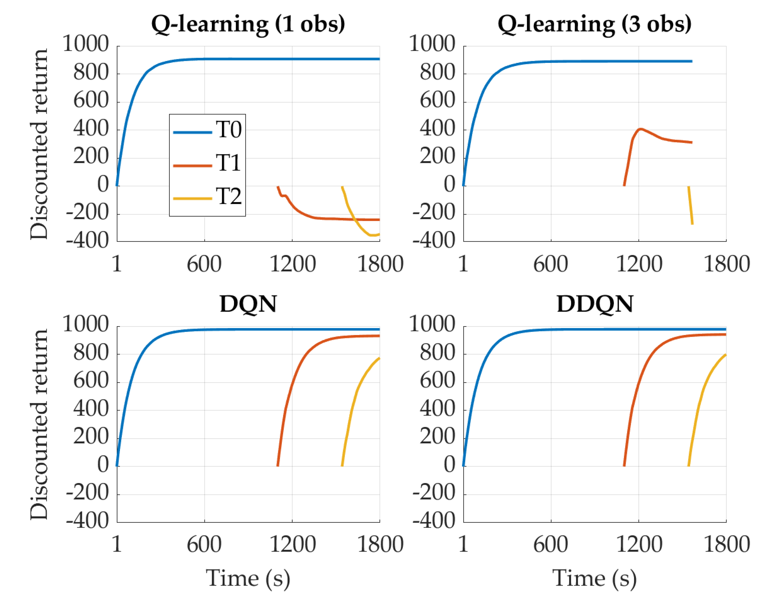
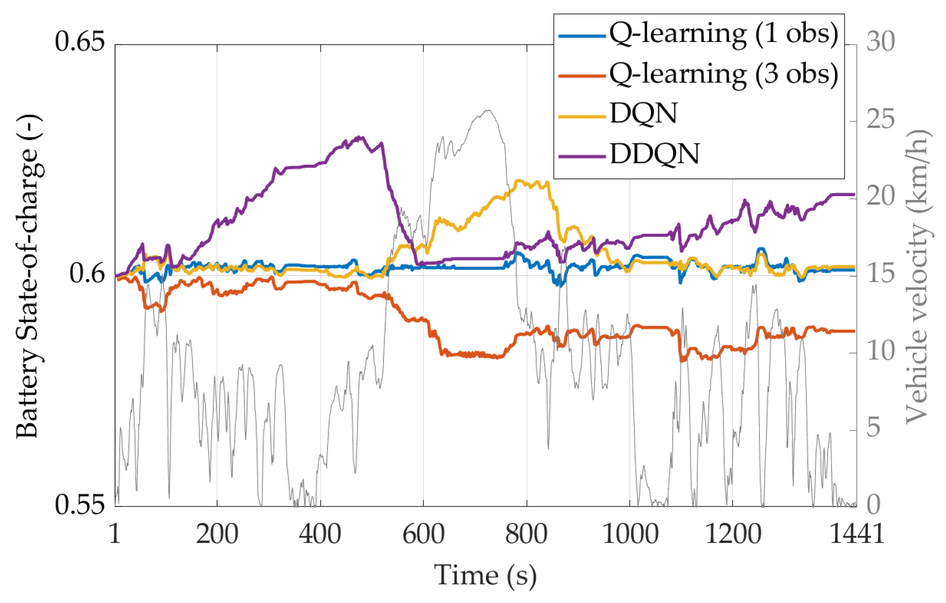
4.3. Testing Reinforcement Learning Agents on a Real-World Driving Mission

Finally, the four RL agents trained on a single type-approval driving cycle were tested on the RDM. The battery SOC trends obtained for the RDM when the agents are trained with a SOC-oriented reward on the FTP-75 and the WLTC are reported in Figure 14 and Figure 15, respectively. As far as the WLTC is concerned (Figure 15), the Q-learning 1 obs and the DQN outperform the DDQN, the latter leading to a final battery SOC value significantly higher with respect to the reference one. On the other hand, the Q-learning 3 obs and the DDQN are clearly outperformed by the Q-learning 1 obs when the training occurs on the FTP-75 (Figure 14). The real FCs are reported in Table 5. The Q-learning 1 obs once more establishes its superiority when a SOC-oriented reward function is adopted.
As far as the FC-oriented reward is concerned, the battery SOC and cumulative FC traces over the RDM are reported in Figure 16 and Figure 17 for the WLTC and the FTP-75 training, respectively. The performances of the RL agents are aligned with the results of the previous Section considering the FC minimization control task. Indeed, the DRL agents are once more capable of outperforming the Q-learning agents. The numerical results related to the plots of Figure 16 and Figure 17 are reported in Table 6, further assessing the dominance of the DRL over the Q-learning agents for the FC-oriented approach.

5. Conclusions

The performances of different RL agents for the real-time control of a full hybrid electric vehicle were assessed considering multiple driving conditions (both regulatory driving cycles and real-world driving missions) and two different reward functions. The latter were selected and considered to push the agents towards different optimization objectives. On the one hand, a SOC-oriented reward function was designed to lead the control policy towards the optimal sustaining mode for the battery state of charge whilst still complying with reduction in fuel consumption (FC). On the other hand, a FC-oriented reward was designed to primarily minimize fuel consumption whilst maintaining the battery SOC within an acceptable range. The agents were initially trained on the WLTC and the FTP-75 and tested for the same driving conditions. The trends in battery SOC, the cumulative FCs, and the learning curves suggest that disconnecting the selection of the RL agent from the actual reward function formulation might lead to non-optimal responses. In fact, for the simpler RL agents, e.g., Q-learning, surprisingly, the SOC-oriented reward leads to to comparable or even better results than with the more sophisticated agents, e.g., the DQN and the DDQN. Dominance of the DQN and the DDQN agents is exhibited only when the FC-oriented reward is considered. In fact, the utilization of more powerful RL agents should only be justified by the increased complexity of the control problem; minimizing fuel consumption while maintaining the battery state of charge within a given range clearly represents a very difficult task to be solved, as demonstrated by the amount of research activities to this end presented in the literature.
The findings of this paper demonstrate the need for RL users to prioritize the selection and tuning of each experiment configuration rather than just relying upon the latest RL agents in the literature. To further support the thesis, the trained RL agents were also tested on real-world driving conditions. Regardless of the training conditions, the results confirm that simple RL agents behave efficiently in the case of a SOC-oriented reward, whereas more sophisticated agents are needed when FC-oriented rewards are considered.

Author Contributions

Conceptualization, C.M. and M.A.; methodology, C.M., M.A., A.M. and L.S.; software, C.M., M.A., A.M. and L.S.; validation, C.M. and M.A.; formal analysis, C.M. and M.A.; investigation, C.M. and M.A.; resources, C.M., M.A., A.M. and L.S.; data curation, C.M. and M.A.; writing—original draft preparation, C.M. and M.A.; writing—review and editing, C.M. and D.M.; visualization, C.M. and M.A.; supervision, E.B., D.M. and E.S.; project administration, E.B., D.M. and E.S. All authors have read and agreed to the published version of the manuscript.

Funding

This research received no external funding.

Data Availability Statement

No new data were created or analyzed in this study. Data sharing is not applicable to this article.

Conflicts of Interest

The authors declare no conflict of interest.

References

  1. Ehsani, M.; Gao, Y.; Longo, S.; Ebrahimi, K. Modern Electric, Hybrid Electric, and Fuel Cell Vehicles; CRC Press: Boca Raton, FL, USA, 2018. [Google Scholar]
  2. Kebriaei, M.; Niasar, A.H.; Asaei, B. Hybrid electric vehicles: An overview. In Proceedings of the 2015 International Conference on Connected Vehicles and Expo (ICCVE), Shenzhen, China, 19–23 October 2015; pp. 299–305. [Google Scholar] [CrossRef]
  3. Biswas, A.; Emadi, A. Energy management systems for electrified powertrains: State-of-the-art review and future trends. IEEE Trans. Veh. Technol. 2019, 68, 6453–6467. [Google Scholar] [CrossRef]
  4. Banvait, H.; Anwar, S.; Chen, Y. A Rule-Based Energy Management Strategy for Plug- in Hybrid Electric Vehicle (PHEV). In Proceedings of the 2009 American Control Conference, St. Louis, MO, USA, 10–12 June 2009; IEEE: New York, NY, USA, 2009; pp. 3938–3943. [Google Scholar]
  5. Musardo, C.; Rizzoni, G.; Guezennec, Y.; Staccia, B. A-ECMS: An adaptive algorithm for hybrid electric vehicle energy management. Eur. J. Control 2005, 11, 509–524. [Google Scholar] [CrossRef]
  6. Huang, Y.; Wang, H.; Khajepour, A.; He, H.; Ji, J. Model predictive control power management strategies for HEVs: A review. J. Power Sources 2017, 341, 91–106. [Google Scholar] [CrossRef]
  7. Ganesh, A.H.; Xu, B. A review of reinforcement learning based energy management systems for electrified powertrains: Progress, challenge, and potential solution. Renew. Sustain. Energy Rev. 2022, 154, 111833. [Google Scholar] [CrossRef]
  8. Cioffi, R.; Travaglioni, M.; Piscitelli, G.; Petrillo, A.; De Felice, F. Artificial intelligence and machine learning applications in smart production: Progress, trends, and directions. Sustainability 2020, 12, 492. [Google Scholar] [CrossRef]
  9. Hu, X.; Liu, T.; Qi, X.; Barth, M. Reinforcement Learning for Hybrid and Plug-In Hybrid Electric Vehicle Energy Management: Recent Advances and Prospects. IEEE Ind. Electron. Mag. 2019, 13, 16–25. [Google Scholar] [CrossRef]
  10. Liu, T.; Hu, X.; Li, S.E.; Cao, D. Reinforcement Learning Optimized Look-Ahead Energy Management of a Parallel Hybrid Electric Vehicle. IEEE ASME Trans. Mechatron. 2017, 22, 1497–1507. [Google Scholar] [CrossRef]
  11. Xu, B.; Rathod, D.; Zhang, D.; Yebi, A.; Zhang, X.; Li, X.; Filipi, Z. Parametric study on reinforcement learning optimized energy management strategy for a hybrid electric vehicle. Appl. Energy 2020, 259, 114200. [Google Scholar] [CrossRef]
  12. Xu, B.; Tang, X.; Hu, X.; Lin, X.; Li, H.; Rathod, D.; Wang, Z. Q-Learning-Based Supervisory Control Adaptability Investigation for Hybrid Electric Vehicles. IEEE Trans. Intell. Transp. Syst. 2021, 23, 6797–6806. [Google Scholar] [CrossRef]
  13. Xu, B.; Malmir, F.; Rathod, D.; Filipi, Z. Real-Time reinforcement learning optimized energy management for a 48V mild hybrid electric vehicle. SAE Tech. Pap. 2019, 2019, 1–9. [Google Scholar] [CrossRef]
  14. Hu, Y.; Li, W.; Xu, K.; Zahid, T.; Qin, F.; Li, C. Energy management strategy for a hybrid electric vehicle based on deep reinforcement learning. Appl. Sci. 2018, 8, 187. [Google Scholar] [CrossRef]
  15. Zhang, S.; Chen, J.; Tang, X. Multi-objective control and energy management strategy based on deep Q-network for parallel hybrid electric vehicles. Int. J. Veh. Perform. 2022, 8, 371–386. [Google Scholar] [CrossRef]
  16. Wu, J.; He, H.; Peng, J.; Li, Y.; Li, Z. Continuous reinforcement learning of energy management with deep Q network for a power split hybrid electric bus. Appl. Energy 2018, 222, 799–811. [Google Scholar] [CrossRef]
  17. Han, X.; He, H.; Wu, J.; Peng, J.; Li, Y. Energy management based on reinforcement learning with double deep Q-learning for a hybrid electric tracked vehicle. Appl. Energy 2019, 254, 113708. [Google Scholar] [CrossRef]
  18. Liu, T.; Wang, B.; Yang, C. Online Markov Chain-based energy management for a hybrid tracked vehicle with speedy Q-learning. Energy 2018, 160, 544–555. [Google Scholar] [CrossRef]
  19. Wu, Y.; Tan, H.; Peng, J.; Zhang, H.; He, H. Deep reinforcement learning of energy management with continuous control strategy and traffic information for a series-parallel plug-in hybrid electric bus. Appl. Energy 2019, 247, 454–466. [Google Scholar] [CrossRef]
  20. Tan, H.; Zhang, H.; Peng, J.; Jiang, Z.; Wu, Y. Energy management of hybrid electric bus based on deep reinforcement learning in continuous state and action space. Energy Convers. Manag. 2019, 195, 548–560. [Google Scholar] [CrossRef]
  21. Biswas, A.; Anselma, P.G.; Emadi, A. Real-Time Optimal Energy Management of Multimode Hybrid Electric Powertrain with Online Trainable Asynchronous Advantage Actor—Critic Algorithm. IEEE Trans. Transp. Electrif. 2022, 8, 2676–2694. [Google Scholar] [CrossRef]
  22. Li, Y.; Tao, J.; Xie, L.; Zhang, R.; Ma, L.; Qiao, Z. Enhanced Q-learning for real-time hybrid electric vehicle energy management with deterministic rule. Meas. Control 2020, 53, 1493–1503. [Google Scholar] [CrossRef]
  23. Maino, C.; Mastropietro, A.; Sorrentino, L.; Busto, E.; Misul, D.; Spessa, E. Project and Development of a Reinforcement Learning Based Control Algorithm for Hybrid Electric Vehicles. Appl. Sci. 2022, 12, 812. [Google Scholar] [CrossRef]
  24. Joshi, A. Review of Vehicle Engine Efficiency and Emissions. SAE Tech. Pap. 2021, 2, 2479–2507. [Google Scholar] [CrossRef]
  25. EPA, United States Environmental Protection Agency. Emission Standards Reference Guide. EPA Federal Test Procedure (FTP). Available online: https://www.epa.gov/emission-standards-reference-guide/epa-federal-test-procedure-ftp (accessed on 29 January 2023).
  26. Fusco, G.; Bracci, A.; Caligiuri, T.; Colombaroni, C.; Isaenko, N. Experimental analyses and clustering of travel choice behaviours by floating car big data in a large urban area. IET Intell. Transp. Syst. 2018, 12, 270–278. [Google Scholar] [CrossRef]
  27. Puterman, M. Markov Decision Processes; John Wiley and Sons: New York, NY, USA, 1994. [Google Scholar]
  28. Fechert, R.; Lorenz, A.; Liessner, R.; Bäker, B. Using Deep Reinforcement Learning for Hybrid Electric Vehicle Energy Management under Consideration of Dynamic Emission Models. SAE Tech. Pap. 2020, 58, 1–13. [Google Scholar] [CrossRef]
  29. Sutton, R.S.; Barto, A.G. Reinforcement Learning: An Introduction; MIT Press: Cambridge, MA, USA, 2018. [Google Scholar]
  30. Watkins, C.J.C.H.; Dayan, P. Q-Learning. Mach. Learn. 1992, 8, 279–292. [Google Scholar] [CrossRef]
  31. Mnih, V.; Silver, D. Playing Atari with Deep Reinforcement Learning. Available online: https://arxiv.org/abs/1312.5602 (accessed on 29 January 2023).
  32. Fan, J.; Wang, Z. A Theoretical Analysis of Deep Q-Learning. Available online: https://arxiv.org/abs/1901.00137v3 (accessed on 29 January 2023).
  33. Fujimoto, S.; Van Hoof, H.; Meger, D. Addressing Function Approximation Error in Actor-Critic Methods. Available online: http://arxiv.org/abs/1802.09477 (accessed on 29 January 2023).
  34. Van Hasselt, H.; Guez, A.; Silver, D. Deep Reinforcement Learning with Double Q-Learning. Available online: http://arxiv.org/abs/1509.06461 (accessed on 29 January 2023).
  35. Sciarretta, A.; Guzzella, L. Control of hybrid electric vehicles. IEEE Control Syst. Mag. 2007, 27, 60–70. [Google Scholar] [CrossRef]
  36. Maino, C.; Misul, D.; Musa, A.; Spessa, E. Optimal mesh discretization of the dynamic programming for hybrid electric vehicles. Appl. Energy 2021, 292, 116920. [Google Scholar] [CrossRef]
Figure 1. Power demand and velocity profile of WLTC (top chart), FTP−75 (mid chart) and RDM (bottom chart) for the identified vehicle.
Energies 16 02749 g001
Figure 2. Battery SOC profiles obtained by the RL agents on the WLTC in the case of SOC−oriented reward.
Energies 16 02749 g002
Figure 3. Battery SOC profiles obtained by the RL agents on the FTP−75 in the case of SOC−oriented reward.
Energies 16 02749 g003
Figure 4. Discounted return profiles per episode obtained by the RL agents on the WLTC in the case of SOC−oriented reward.
Energies 16 02749 g004
Figure 5. Discounted return profiles per episode obtained by the RL agents on the FTP−75 in the case of SOC−oriented reward.
Energies 16 02749 g005
Figure 6. Discounted return profiles through time obtained by the RL agents on the WLTC at episode 100 in the case of SOC−oriented reward.
Energies 16 02749 g006
Figure 7. Discounted return profiles through time obtained by the RL agents on the WLTC at episode 1000 in the case of SOC−oriented reward.
Energies 16 02749 g007
Figure 8. Battery SOC (upper chart) and FC (lower chart) profiles obtained by the RL agents on the WLTC in the case of FC−oriented reward.
Energies 16 02749 g008
Figure 9. Battery SOC (upper chart) and FC (lower chart) profiles obtained by the RL agents on the FTP−75 in the case of FC−oriented reward.
Energies 16 02749 g009
Figure 10. Discounted return per episode profiles obtained by the RL agents on the WLTC in the case of FC−oriented reward.
Energies 16 02749 g010
Figure 11. Discounted return per episode profiles obtained by the RL agents on the FTP-75 in the case of FC−oriented reward.
Energies 16 02749 g011
Figure 12. Discounted return profiles through time obtained by the RL agents on the WLTC at episode 100 in the case of FC−oriented reward.
Energies 16 02749 g012
Figure 13. Discounted return through time profiles obtained by the RL agents on the WLTC at episode 1000 in the case of FC−oriented reward.
Energies 16 02749 g013
Figure 14. Battery SOC profiles obtained by the RL agents on the RDM when trained on the FTP−75 in the case of SOC−oriented reward.
Energies 16 02749 g014
Figure 15. Battery SOC profiles obtained by the RL agents on the RDM when trained on the WLTC in the case of SOC−oriented reward.
Energies 16 02749 g015
Figure 16. Battery SOC (upper chart) and FC (lower chart) profiles obtained by the RL agents on the RDM when trained on the WLTC in the case of FC−oriented reward.
Energies 16 02749 g016
Figure 17. Battery SOC (upper chart) and FC (lower chart) profiles obtained by the RL agents on the RDM when trained on the FTP−75 in the case of FC−oriented reward.
Energies 16 02749 g017
Table 1. Vehicle data.
General Specifications
Vehicle classPassenger car
Kerb weight (kg)750
Vehicle mass (w/pwt components)1200
Transmission6-gears
Internal Combustion Engine
Fuel typeGasoline
Maximum power (kW (@ rpm))88 (@ 5500)
Maximum torque (Nm (@ rpm))180 (@ 1750–4000)
Rotational speed range (rpm)0–6250
Motor-Generator
Maximum power (kW (@ rpm))70 (@ 6000)
Maximum torque (Nm (@ rpm))154 (@ 0–4000)
Rotational speed range (rpm)0–13,500
Battery
Peak power (kW)74
Energy content (kWh)6.1
AC/DC converter efficiency (-)0.95
Table 2. Setup of the experiments.
HyperparametersValues
Training episodes1000
Discount factor0.99
Learning rate (Q-learning)0.9
Learning rate (DNNs)2 × 10⁻⁴
Exploration rate @ E = 10.8
Minimum exploration rate @ E = 10.05
Update frequency of target network6000
Mini-batch size32
Experience replay memory size100,000
Number of hidden layers (DNNs)1
Neurons in the hidden layers (DNNs)64
Reward coefficient a 10
Reward coefficient b (SOC-oriented)−1000
Reward coefficient b (FC-oriented)−3000
Reward coefficient c (SOC-oriented)−1000
Reward coefficient c (FC-oriented)−150
Reward penalty p −100
Table 3. Results for the SOC−oriented reward.
Agent M f   ( g ) S O C T   ( ) M f , r   ( g ) M f , r   ( % )
WLTC
Q-learning (1 obs)8220.614822-
Q-learning (3 obs)8150.585836−1.66
DQN8450.616845−2.77
DDQN8630.620863−4.93
FTP-75
Q-learning (1 obs)3680.604368-
Q-learning (3 obs)3760.589392−2.20
DQN3630.6023631.52
DDQN3620.6093621.77
Table 4. Results of the FC−oriented reward.
Agent M f   ( g ) S O C T   ( ) M f , r   ( g ) M f , r   ( % )
WLTC
Q-learning (1 obs)9540.603954-
Q-learning (3 obs)----
DQN7260.58075321.07
DDQN7210.60272124.41
FTP-75
Q-learning (1 obs)3350.570378-
Q-learning (3 obs)3130.5713556.08
DQN3370.60133710.85
DDQN3130.58932912.96
Table 5. Results of the testing on RDM for the SOC−oriented reward.
Agent M f   ( g ) S O C T   ( ) M f , r   ( g ) M f , r   ( % )
Train WLTC—Test RDM
Q-learning (1 obs)4360.601436-
Q-learning (3 obs)4470.599448−2.75
DQN4630.619463−6.19
DDQN4070.6044076.65
Train FTP-75—Test RDM
Q-learning (1 obs)3940.601394-
Q-learning (3 obs)4160.588433−9.90
DQN4040.602404−2.54
DDQN4590.617459−16.50
Table 6. Results of the testing on RDM for the FC−oriented reward.
Agent M f   ( g ) S O C T   ( ) M f , r   ( g ) M f , r   ( % )
Train WLTC—Test RDM
Q-learning (1 obs)5160.595523-
Q-learning (3 obs)3880.58241420.84
DQN3840.59938526.39
DDQN3720.60237228.87
Train FTP-75—Test RDM
Q-learning (1 obs)3970.594406-
Q-learning (3 obs)3700.569415−2.22
DQN3820.6023825.91
DDQN3540.5923669.85
Disclaimer/Publisher’s Note: The statements, opinions and data contained in all publications are solely those of the individual author(s) and contributor(s) and not of MDPI and/or the editor(s). MDPI and/or the editor(s) disclaim responsibility for any injury to people or property resulting from any ideas, methods, instructions or products referred to in the content.

