Review

High Impedance Fault Models for Overhead Distribution Networks: A Review and Comparison with MV Lab Experiments

by
Juan Carlos Huaquisaca Paye
1,2,*,
João Paulo A. Vieira
1,
Jonathan Muñoz Tabora
1,3,
André P. Leão
1,
Murillo Augusto M. Cordeiro
1,
Ghendy C. Junior
4,
Adriano P. de Morais
4 and
Patrick E. Farias
5
1
Institute of Technology, Electrical Engineering Faculty, Federal University of Pará, Belém 66075-110, Brazil
2
Electrical Engineering Department, The Public University of El Alto (UPEA), La Paz 00591, Bolivia
3
Electrical Engineering Department, National Autonomous University of Honduras (UNAH), Tegucigalpa 04001, Honduras
4
Department of Electrical Engineering, Federal University of Santa Maria, Santa Maria 97105-900, Brazil
5
Federal Institute of Education, Science and Technology, Federal Institute of Rio Grande do Sul, Farroupilhas 95174-274, Brazil
*
Author to whom correspondence should be addressed.
Submission received: 31 December 2023 / Revised: 2 February 2024 / Accepted: 6 February 2024 / Published: 27 February 2024

Abstract

:
Detecting and locating high impedance faults (HIF) in overhead distribution networks (ODN) remains one of the biggest challenges for manufacturers and researchers due to the complexity of this phenomenon, where the electrical current magnitude is similar to that of the loads. To simulate HIF, the selection of the HIF model is important, because it has to correctly reproduce the characteristics of this phenomenon, so that it does not negatively influence the simulations results. Therefore, HIF models play a fundamental role in proposing solutions and validating the effectiveness of the proposed methods to detect and localize HIF in ODN. This paper presents a systematic review of HIF models. It is intended to facilitate the selection of the HIF model to be considered. The models are validated based on experimental data from medium voltage (MV) laboratories, specifically, recorded waveforms from two HIF tests conducted in an MV lab were analyzed and compared with three established HIF models. The efficacy of these models was assessed against MV lab test data to ensure a precise representation of both transient and steady-state conditions for fault conductance and current waveforms. The findings show that the two nonlinear resistor models better approximate the waveforms obtained in the experimental tests performed in this study.

1. Introduction

1.1. General Considerations

A high impedance fault (HIF) is defined as a disturbance caused by a conductor that touches a high-resistance nonmetallic surface connected to the ground, producing an arcing fault current lower than the residual relay pickup setting. According to [1], HIFs involving downed conductors in contact with a surface, correspond to 10% of all faults occurring in overhead distribution networks (ODN) [1]. The percentage of HIFs in ODN is even higher since not all HIF events are reported [2]. In addition, HIFs can occur without rupture or downfall of conductors on a surface, therefore, the HIF current is so low that it cannot be detected by conventional overcurrent protection functions [3]. This protection issue has been a challenge for distribution utility engineers for a long time [4]. To further complicate matters, HIF current waveforms have diverse characteristics, such as asymmetry, nonlinearity, build-up, shoulder, intermittence, and randomness [5].
High impedance faults in ODN may cause serious and harmful effects, such as (1) risk of electric shock; (2) risk of fire in material assets and forests; (3) electricity supply interruptions; and (4) long service restoration times. These effects continuously motivate the development of new ideas and innovative solutions for HIF detection and location, since they are challenging issues remaining unsolved or partially solved by the power distribution industry. In that sense, more reliable algorithms for HIF studies should be developed based on the above-mentioned HIF current waveform characteristics, which can be represented by mathematical models that can reproduce them.
Test data from many early staged HIF studies have provided valuable information toward understanding and characterizing HIFs [6,7]. To test the effectiveness and robustness of these algorithms, time-domain computational simulations must be performed considering the asymmetric, nonlinear, intermittent, and random nature of the HIF phenomenon. It is worth highlighting that HIFs are a random and dynamic phenomenon since they produce arcing and flashing at the point of contact, and the conductor may move around due to electromagnetic force [8].
The use of accurate HIF models for purposes of designing and testing HIF detection and location algorithms is essential. HIF computational simulations can provide, at the very least, initial data for preliminary research. On the other hand, field tests on an actual medium voltage (MV) distribution network are not a recommended practice due to the inherent danger involving this type of arcing fault in an uncontrolled environment.
Modeling of HIFs in ODN can be classified into three main categories: (1) model based on active and passive circuit elements; (2) model based on passive circuit elements; and (3) arcing model. Modeling based on active and passive circuit elements was proposed by [9] and analyzed in [10]. The model is based on antiparallel diodes and its parameters are considered to remain constant during the analyzed period. However, this model cannot reproduce transient-state conditions of the HIF current waveform. A model based on passive circuit elements was introduced by [11]. Some proposed modifications by [12] were included in the model, which allows to simulate HIF on different types of ground surfaces. Yet, this model depends on the V × I curve at the HIF point for each type of ground surface. The arcing model was initially introduced by [13,14] in the form of a first-order differential equation. This model is a simple physical representation that describes the behavior of an electric arcing. In the last years, arcing models have been investigated in [15,16]. However, representing HIFs by arc models that can reproduce varied characteristics of the phenomenon is not always possible, which motivates the research in HIF modeling.

1.2. Motivation and Contribution

In the literature there are works related to the review of HIF detection and localization techniques [5,17,18,19], but the main goal is not to analyze HIF models. And the works that include HIF models [10,20], do not perform a validation of the analyzed models, on the other hand, some authors only validate the selected model separately [12,16,21,22], without comparing the waveform reproduction, using the different HIF models that exist in the literature. In that sense, the main contributions of this work are:
  • A systematic review of existing works on HIF models for ODN with a critical analysis on reproducing HIF characteristics. The paper shows the evolution, popularity, limitations, advantages, and disadvantages of HIF models. As a result, researchers and specialists can save time in the selection of the appropriate HIF model for their studies.
  • The primary contribution of this work is the comparison of three well-known HIF models for ODN with actual experiments conducted in a high-voltage laboratory at the Federal University of Para. This analysis highlights both the strengths and limitations of these models across various applications.
The motivation and contribution of this study arise from the limitations that the authors may experience at the beginning of the research on issues developed in HIF, as occurred in previous studies presented by the authors in [21,23,24,25,26,27,28]. Based on the above, this study contributes directly to the proposal and validation of the most appropriate detection or localization method in HIF.

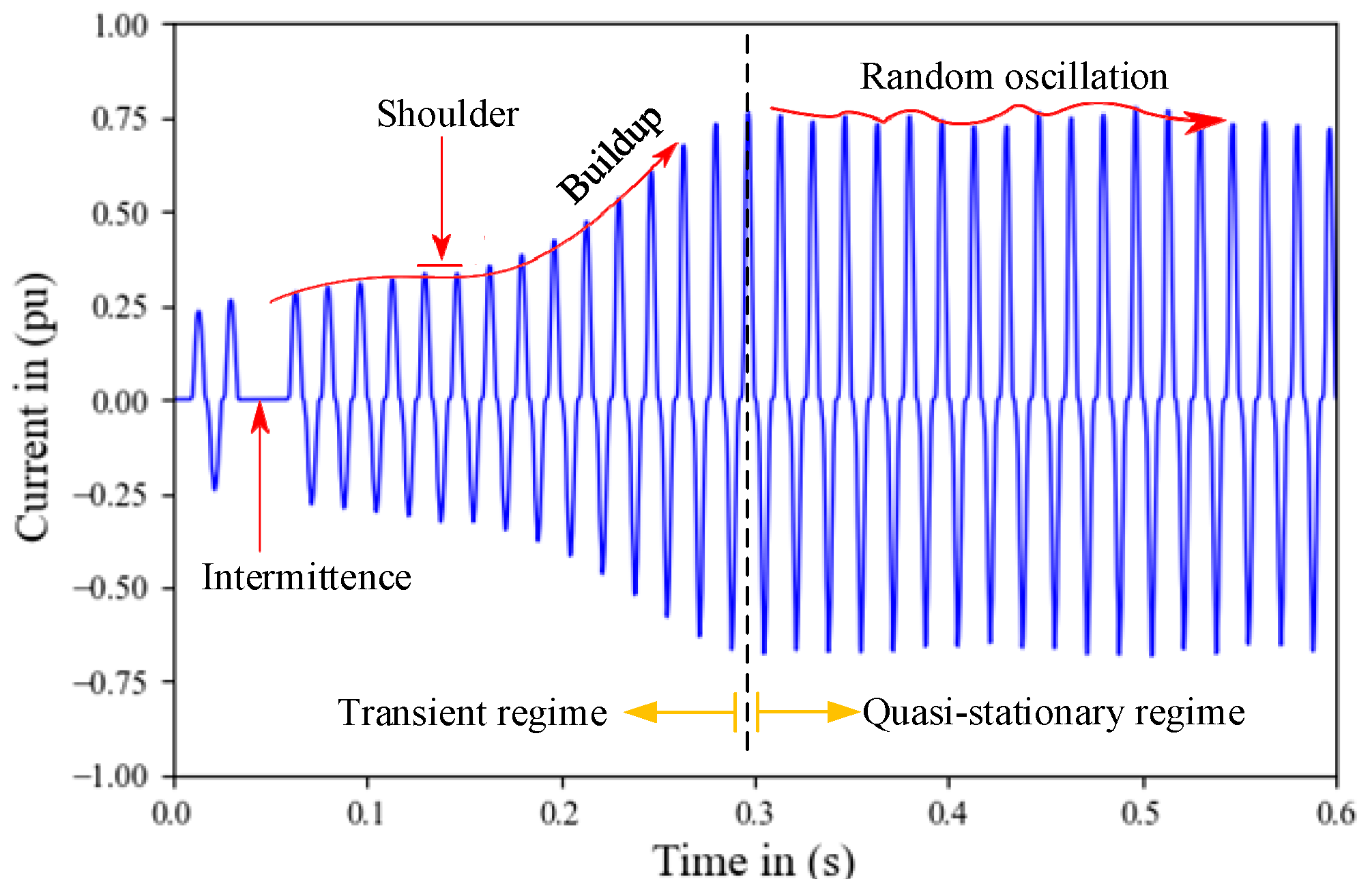
2. High Impedance Fault Characteristics

The HIF characteristics contained in the current waveform, as defined follow:
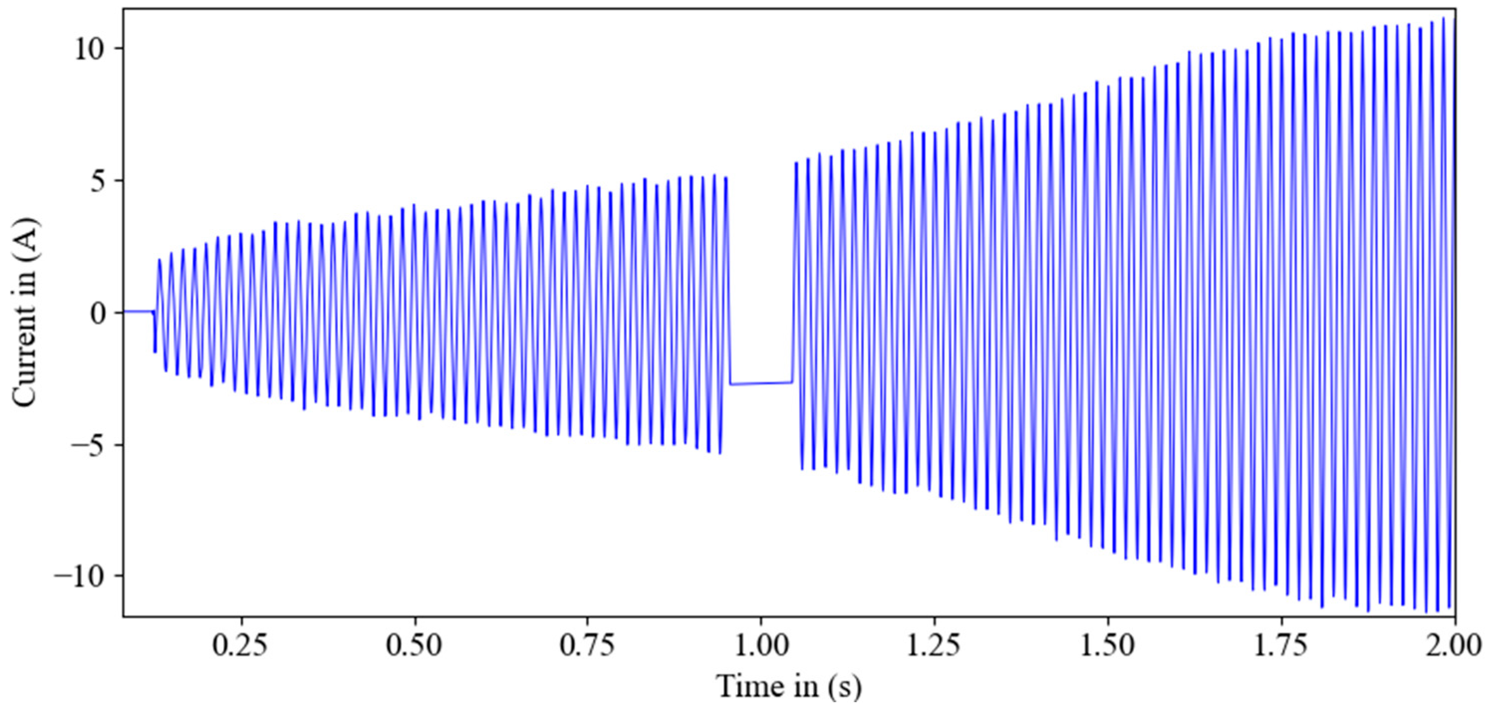
  • Asymmetry: Peak values of current are different in the positive and negative half cycle. The asymmetric nature of HIF current is influenced by the porosity and moisture of the surface contact. The presence of silica in the contact surfaces causes asymmetry, according to [9]. The heated silica forms a type of cathode spot that absorbs electrons, causing voltage drops when the cable is subjected to a positive voltage.
  • Nonlinearity: Voltage x current characteristic curve is highly nonlinear. This characteristic is caused by the electric arc associated with the nonlinearity of high-impedance objects [9,29,30].
  • Build-up: HIF current magnitude gradually increases up to its maximum value. This is due to: (a) the physical accommodation of the cable in the soil, since the cable can move or settle into the soil [12,13,14,15,16,17,18,19,20,21,22,23,24,25,26,27,28,29,30,31]; and (b) the arc penetrates the soil surface and causes soil ionization, increasing the effective area of the equivalent electrode [30].
  • Shoulder: HIF current magnitude maintains constant right after the Build-up end.
  • Intermittence: HIF electric arc is extinct during a time due to the loss of moisture in the surface and physical accommodation of the cable.
  • Randomness: Peak values of current randomly oscillate at each half cycle within a relatively small range due to the random behavior of the electric arc.
Describe these characteristics related to [7], published in 1982. The works in [12] and in general, works addressing HIFs in ODN describe the first five characteristics of HIF mentioned above, since they are consolidated in the literature [32,33]. The randomness characteristic of a HIF, mentioned in [15,34,35,36,37,38], is manifested by a random oscillation in the HIF current waveform. In the technical literature, the characteristic of randomness and some others can be observed in actual HIF current waveforms presented in [11,12,15,34,37,38,39,40,41,42,43], in which the randomness issue is not addressed [11], among others, consider that the HIF current waveform can be divided into two distinct conditions: transient and steady-state conditions. Some HIF models only consider the steady-state condition, in which the HIF current waveform of a cycle is repeated over time. The transient state condition lasts only the first few cycles, during the build-up. The steady-state condition starts after the build-up end. The nonlinearity and asymmetry characteristics are contained in the steady-state current waveforms. The presence of randomness in the HIF current waveform leads the steady-state condition to a quasi-steady-state condition, as shown in Figure 1. It is observed that, after the current peaks build up, a random oscillation appears. HIF current peak values are within a standard deviation. This characteristic of randomness is contained practically in any HIF current waveform.
References [5,34,38,44] mention other characteristics contained in the HIF current waveform. However, this paper does not focus on other characteristics, since they are dependent on the main characteristics (e.g., the harmonic content depending on the nonlinearity characteristic). According to [30], HIFs are considered single-phase faults because an incident involving two or more phases is typically a high current fault event or can be treated as two isolated single-phase HIF events. Also, it should be borne in mind that the HIF current is exactly in phase with the voltage at the fault point and the resulting harmonic currents tend to reach their peaks at the same time as the HIF current fundamental component, according to [30,45,46].

3. Categories of HIF Models for ODN

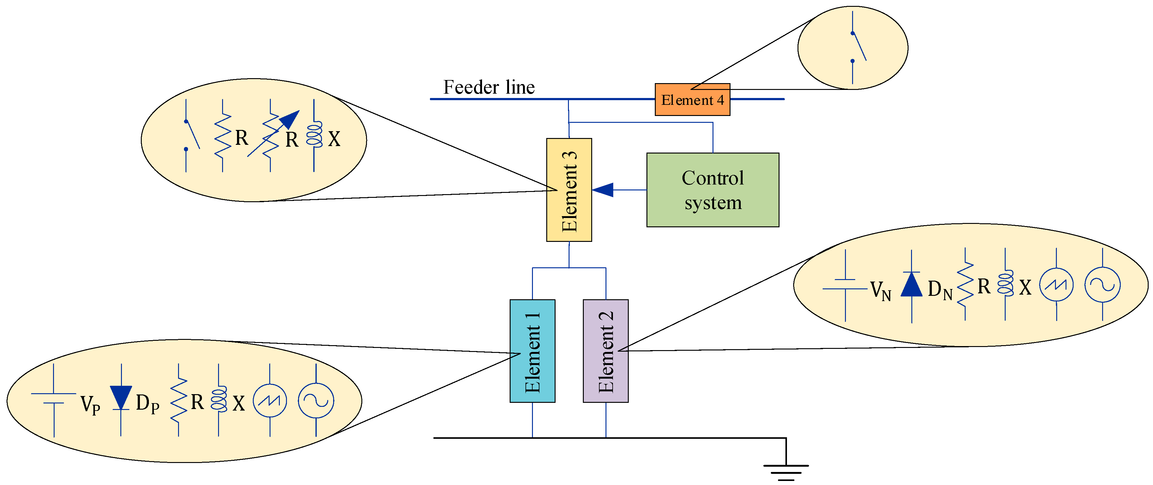
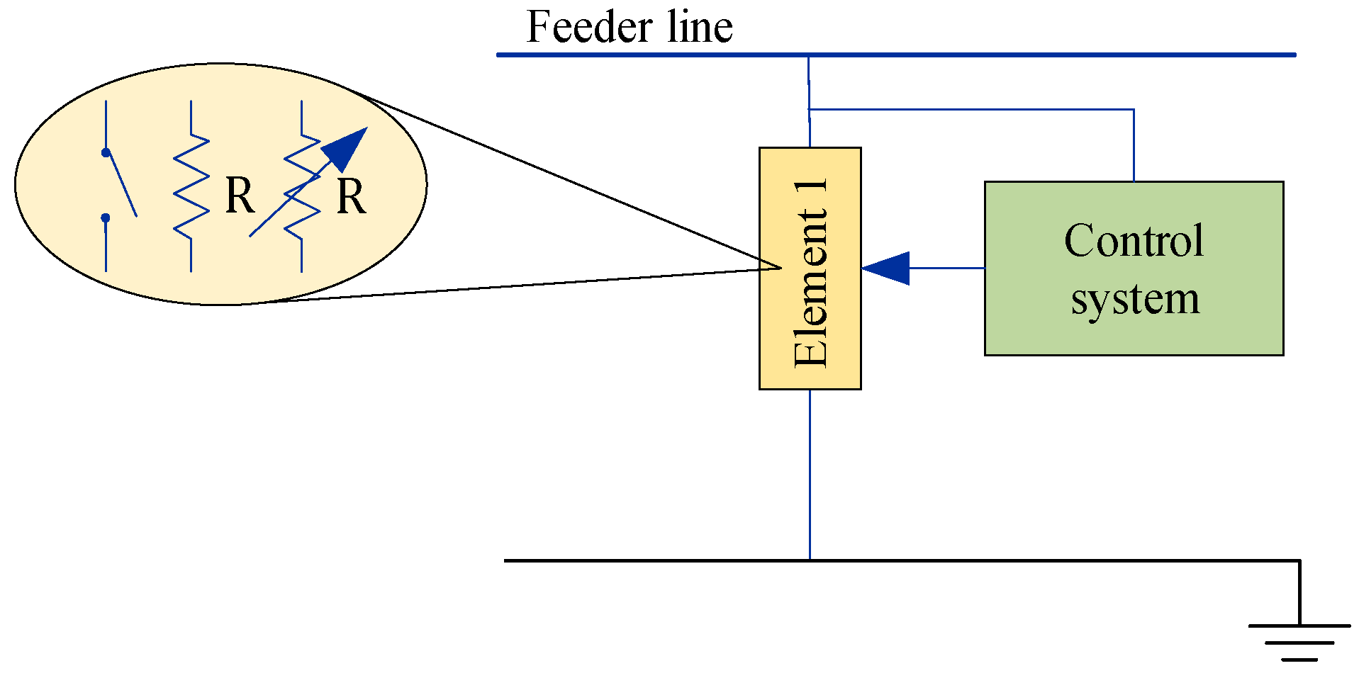
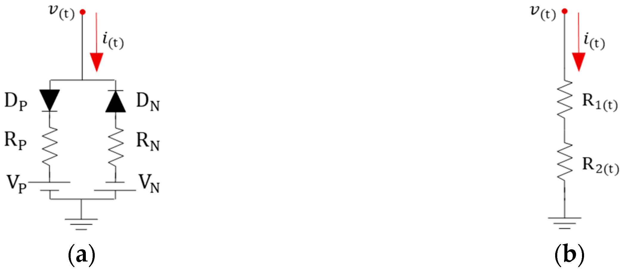
3.1. Models Based on Active and Passive Circuit Elements

This section shows the evolution of the models of active and passive circuit elements used in the studies of the last 30 years for each HIF model in the ODN, classified in terms of their elements, representation and year of publication. The base model (model “a”) and the rest of the models in this category can be constructed using Figure 2 and Table 1. Figure 2 shows the different active and passive elements that can be connected in series within elements 1, 2, 3 and 4. For example, in model “a”, element 1 consists of a DC voltage source ( V P ) and a diode ( D P ) connected in series. Element 2 consists of a DC voltage source ( V N ) and a diode ( D N ) connected in series, and element 3 consists of a resistor ( R ) and an inductor ( X ) connected in series.
The electrical circuit elements that compose a HIF model consist of a constant impedance (resistance R and reactance X ) in series with two antiparallel diodes ( D P and D N ). Each diode is in series with a DC voltage source ( V P or V N ). This antiparallel-diode configuration allows the current during positive half cycles to circulate only through one branch and the current during negative half cycles flows through another branch. The fault current magnitude is controlled by the impedance value, but the source voltage values also influence the current magnitude control, as observed in Figure 3, which presents simulation results to understand the behavior of the model proposed in [9].
In Figure 3a, the variation of the current for different values of voltage V N are presented, where: V N 1 < V N 2 < V N 3 , maintaining both constant impedance and constant voltage VP. It can be concluded that the variable parameter ( V N ) simultaneously modifies the current magnitude and the current conduction instants during negative semi-cycles (the three currents are superimposed during positive semi-cycles). By analogy, this behavior will be repeated during the positive semi-cycle, but varying VP. Therefore, the variations of VP and VN only affect their respective semi-cycles. Figure 3b shows the current variation for different resistance values, where R 1 < R 2 < R 3 , keeping constant the voltage values of the DC source ( V P and V N ). It is clearly observed that the variable parameter influences on current during two half-cycles and controls the current magnitude. It is important to note that the phase angle difference between the voltage at the fault point and the fault current is negligible, as indicated in the previous section. This fact must be considered to assign a minimum value of inductive reactance to models that consider this element.
As described in Section 2, the HIF current changes over time. However, in the model based on active and passive circuit elements, when it considers constant parameters from the beginning to the end of the simulation, produces a current waveform in which all cycles are equal over time, not allowing full reproduction of this characteristic. Regarding the non-linearity characteristic of HIF, the model does not reproduce this characteristic in the complete cycle, the linearity is maintained within the HIF current conduction intervals. Therefore, this model does not fully reproduce this feature, a fact that can be seen in Figure 4, where the current waveform of a typical HIF is shown, as well as the waveform reproduced from simulations (with the model "a” of Table 1) for a given voltage.
In 1993, the model proposed in [9], derived from works [47,56], is modified as shown in the model “b”, of Table 1. The reactance is neglected, and a resistance is considered in each branch ( R P and R N ), allowing independent control of the current magnitude at each half cycle, but without solving other model limitations.
Reference [57] clearly shows how to reproduce different fault current magnitudes, asymmetries, arc extinctions and arc restarts by modifying V P , V N , R P and R N . A model proposed later in [51,58] does not neglect the reactance, unlike [9], but it considers a resistance for each branch, as observed in the model “f” of Table 1, represented in Figure 2. The work in [59] proposes two non-linear resistances R P and R N , as observed in the model “b” of Table 1 in Figure 2, but it does not provide knowledge of this characteristic. With this proposal, the non-linear characteristic can be reproduced in the conducting and non-conducting intervals as presented in Figure 4. Since HIF is a random and nonlinear phenomenon, authors in [60,61,62,63,64] propose that the parameters VP, VN, RP and RN vary randomly between certain limits at each time interval (ms), following a uniform and/or Gaussian distribution.
The use of random values for elements of this model has been extended to several studies, such as [65,66,67,68]. By proposing the time-varying parameters, the fault current waveform is no longer the same as that of the other cycles. However, the build-up and shoulder characteristics are not guaranteed due to random behavior. Modified models of [9], configured in parallel, are proposed in [52,69] (see model “g” of Table 1 represented in Figure 2). The energization of each of the models in parallel is done by employing switches. According to the authors, this model can reproduce the characteristics of randomness and build-up but adding a greater number of parameters and a switching control system.
In [48,53], DC sources are replaced by sawtooth waveform generators (see models “c” and “h” of Table 1 represented in Figure 2), to control the phase difference between the voltage at the fault point and the fault current. But as described in Section 2, it is not necessary to control this difference, because it is negligible. In addition, a variable resistance is added to the model. In the model in Figure 2, switch 1, normally open, isolates the downstream load from the fault point, and switch 2, normally closed, connects the HIF model to the electrical system. Switch 3 controlled by TACS controls the re-ignition and extinction of the electric arc, to reproduce the intermittency, which is one of the main characteristics of the HIF.
Afterwards, in [54], it is proposed to randomly modify the value of the resistance, in each cycle, and the model is according to the model “i” of Table 1. The references described ([48,53,54]) are not intended to reproduce buildup and other features. In [49,70], the reactance of the model proposed in [9] is neglected and the fixed resistance becomes a non-linear resistance, as can be observed in the model “d” of Table 1, represented in Figure 2. In [49], the voltage values of the DC sources vary randomly at each half-cycle. In [70], the resistance value varies randomly under a uniform distribution. However, in [49] there is the problem of dependence between the beginning of the current conduction and the magnitude of the current waveform, as can be observed in Figure 3a. The HIF models proposed in [49,70] reproduce the current waveform nonlinearity and the current magnitude random behavior.
In [50], a model modification is proposed based on a combination of the model proposed in [9] with the arc model based on a differential equation, according to the model “e” of Table 1. This model is based on works [9,48,71]. Some new features have been added to the model, such as the impedance from [9] which has been replaced by a linear resistor and a time-varying non-linear resistor, representing the earth resistance and the dynamic arc, respectively. AC sources have also been added to the model guaranteeing the variable point of arc ignition and cooling. This model is not simple, since it is practically the union of two models classified into different categories. Therefore, the model complexity is increased due to the greater number of elements composing the model.
In [55], the constant resistance of the model from [9] is replaced by a time-varying resistance to correctly simulate the build-up and shoulder. The model remained simple, as can be observed in the model “j” of Table 1 in Figure 2. The time-varying resistance is modeled by a polynomial function and a constant for transient and quasi-steady states, respectively.
The modeling proposed in [55] can be associated with [11]. In reference [39], regarding the circuit configuration, a resistance is added to each branch that represents the arc resistance. In reference [72], the model proposed in [9] is adapted to be used in the frequency domain, demonstrating the importance of this modeling in the literature. In short, this HIF model can reproduce the characteristics of asymmetry, nonlinearity, build-up, and shoulder considering transient and quasi-steady states.
The model “k” in Table 1, represented by Figure 2 shows the last model based on the combining of electric circuit elements, which was proposed in [31]. It is basically the model proposed in [9] with some features of other models. The main difference is that the model proposed in [31] has a complex control system of resistance and a sectionalizing switch that controls the current circulation. The resistance consists of three portions that add up to the total resistance value. The first portion is established to reproduce the build-up. The second portion is responsible for simulating the asymmetry between half cycles of the same cycle. Finally, the last part reproduces the arc resistance variation, similarly to [11].
It is important to highlight that the evolution of this category of HIF models has not been independent of other categories. Some features present in models of other categories have helped in the evolution of models in this category and vice-versa. A clear example is the way described in [11] to model the build-up and shoulder.
An important observation is that, when this category of HIF models is used, the fault current waveform does not faithfully reproduce waveforms of an actual HIF, especially in the vicinity of zero crossings. In Figure 4, it can be observed the difference between the simulated current (Isim) using the model from [9] and the typical current (Ityp) for a type of surface (e.g., gravel). It is worth noting that the nonlinear resistance can reproduce nonlinearity in the current conduction interval, but not in the non-conduction interval. Last, when DC sources are considered in the model, the reproduced current has limitations in the zero-crossing.

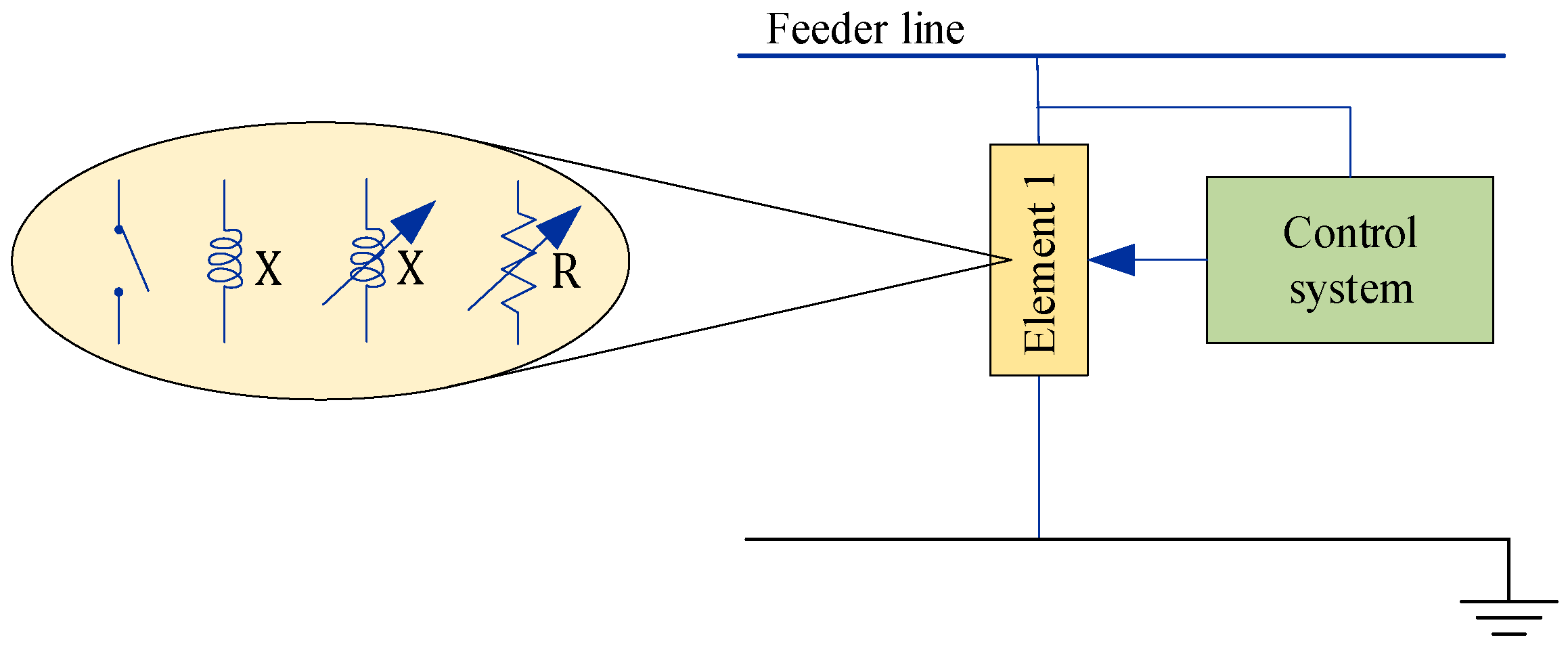
3.2. Models Based on Passive Circuit Elements

Figure 5 and Table 2 illustrates a representation of the different HIF models based on passive elements such as resistance and/or reactance. It can be observed that the evolution of this category of models is not based on a single model, unlike the evolution of models presented in Section 3.1. First, in 1981, authors in [73] proposed a HIF model based on two series nonlinear resistance as a function of the current as shown in the model “a” of Table 2 and represented in Figure 5.
One resistance represents the arc resistance, and the other represents the earth resistance. Subsequently, in [74], HIF is modeled by a resistance and an inductance, both non-linear as a function of the current, subject to a second-order polynomial, as can be observed in Figure 5 and the model “b” of Table 2. Similarly, in [75], HIF is simulated in two ways: (a) constant resistance and reactance; and (b) non-linear resistance as a function of current and constant reactance, as can be observed in Figure 5 and model “d” of Table 2. These models have a common ability to reproduce the characteristic of nonlinearity.
In 1985, the work in [76] used the simplest model consisting of a constant resistance connected at the fault point. This model reproduces only the low HIF magnitude. In recent years, some authors used this model, such as [77], published in 2015. Afterward, the authors in [78] proposed a model based on a combination of 16 nonlinear impedances with different degrees of nonlinearity and with an arc start for different voltage values. HIF simulations can be performed by applying any combination of 16 impedances, that is, one impedance is used for each half-cycle of the voltage waveform. However, this model reproduces with limitations in the shoulder and build-up characteristics through a combination sequence that increases the model complexity. In reference [45], the random nature of the arc has stochastically been simulated using the MODELS language in ATP software (Model “c” of Table 2 and Figure 5). This model consists of a normally open switch connected in series with a variable fault resistance to produce a variety of fault current waveforms each half cycle. After the fault starts, periodic switching operations are determined by the voltage values of the corresponding arc, chosen randomly for each half cycle. This model has the ability to reproduce the intermittency characteristic, but the reproduction of the build-up and shoulder characteristics is not guaranteed due to the stochastic simulation.
The work in [11], published in 2001, presents the most important HIF model this category of models based on passive elements, illustrated in Figure 5 and Table 2, model “e”, since it is capable of reproducing several characteristics of HIF. This model consists of two nonlinear resistances in series, one resistance is responsible for simulating the asymmetry and nonlinearity characteristics, and the other resistance is controlled by TACS to simulate the build-up and shoulder characteristics. The two resistances are determined from curves of voltage at the fault point versus fault current.
In reference [12], published in 2013, the model from [11] is combined with the configuration of switches proposed by [48] (see model “c” of Table 1 in Figure 2), and switches S1 and S2 are used for disconnecting downstream load from the fault point and connecting the HIF model at the fault point, respectively. In reference [12], experimental tests were carried out to establish HIFs of six surface types. The test results were used to model each HIF associated with a surface type. Subsequently, ref. [79] has proposed a control in the switch S3 to simulate the intermittency characteristic. Switch operations are the same adopted in [48], as seen in model “c” of Table 1 in Figure 2. The evolution of this model allows us to reproduce five basic HIF characteristics described in Section 2. Reference [80] proposes the use of two series connected resistors, one dielectric resistance and the other constant bad contact resistance between the conductor and dielectric. The dielectric resistance behavior is based on the solid dielectric electrical breakdown theory. The author shows that the proposed nonlinear resistance model is more consistent in reproducing current waveform at zero-crossing points than the traditional arc model based on differential equations (Mayr model). However, the work does not show the reproduction of the build-up and shoulder characteristics.

3.3. Arc Model

This subsection presents the third category of HIF modeling, which is expressed in the form of a first-order differential equation and represented by the Figure 6 and the Table 3. This HIF model is well known as the arc equation and basically consists of: (1) a single resistance subject to the arc model, as illustrated in Figure 6 and model “a” of Table 3; and (2) two resistances, one that represents the arc resistance (modeled by a differential equation) and the other that can be a constant resistance, shown in Figure 6 and model “b” of Table 3, or a variable over time, shown in Figure 6 and model “c” of Table 3, which represents the resistance of a surface. According to [22], the thermal model has been used since the first descriptions of the arc electrical conductivity shown by Cassie [13] and Mayr [14], in the form of a first-order differential equation. This model has subsequently been improved and modified according to needs. For example, ref. [81] details the implementation of the arc model described in [71] using EMTP. Known as the arc digital model and derived from the description of Hochrainer’s arc, the model from [71] is derived from the works of Mayr and Cassie.
In [82], HIF is modeled by a single resistance based on the first-order differential equation in (1), as originally proposed in [71]. To simulate the random behavior of the phenomenon, the arc voltage per unit length parameter of the differential equation assumes random values within pre-defined limits (G0 is a function of the arc voltage per unit length parameter). In reference [22], HIF is also modeled using the detailed arc description from [71], and to implement the model, the implementation method from [81] is used. Reference [22] models a HIF caused by the cable contact with the tree. This model is represented by two resistances in series, one constant that represents the tree resistance and the other variable that represents the arc resistance.
d g ( t ) d t = G 0 g ( t ) τ
where G0 is stationary arc conductance, τ is arc time constant, and g(t) is time-varying arc conductance [22,71].
In works [83,84], two variable resistances in series are used, one that represents the surface resistance varying between two limits and the other that represents the arc resistance modeled by Equation (1). To reproduce the randomness characteristic, parameter τ takes random values with uniform distribution within predefined limit values.
References [15,85,86] model the HIF based on the Equation (1), whose parameters are obtained from the voltage waveform at the fault point and fault current waveform using the least squares method and the sum of squared deviations from theoretical and experimental values. In these works, the reproduction of nonlinearity and build-up characteristics can be observed. Among works addressing HIF modeling based on the arc model, ref. [15] is recommended because the model is described in a detailed way, showing the calculation of differential equation parameters. Reading [22] is also recommended. Finally, it is worth mentioning that, according to [80], the model based on the arc equation is not consistent in reproducing the HIF waveform at zero-crossing points (see Figure 3 in [80]) and therefore it has a similar limitation to models of the first category.

4. High Impedance Fault Models for ODN

The interaction between any HIF model with an ODN can be illustrated in Figure 7. The configurations of switches S1, S2, and S3 are based on [48]. The switches S1, S2, and S3 allow to simulate different HIF classes. Under normal system conditions, S1 and S2 are normally closed and S3 is normally open. In the case of a load-side HIF, S1 is normally open and S2 and S3 are normally closed, while if the fault is from the source side, S1 and S3 are closed, and S2 is open, in both scenarios there is a similarity between the waveform, both from the source and from the load, as analyzed in [87]. It is also possible to simulate the cable downfall time, which is represented by the time S3 takes to close. For faults involving the unbroken conductor in contact with a tree branch, the three switches are normally closed. It is worth highlighting that S3 has two functions, one that is to connect the HIF model to the distribution system model and the other that is to simulate the intermittence characteristic.
Figure 8a,b show the circuits that represent categories of HIF models based on a combination of electric circuit elements and passive elements, respectively. In the category of models based on a combination of electric circuit elements, the parameter values can be modified to reproduce other models in the same category.
For example, making R P = R N , the circuit model of Figure 8a reproduces the same behavior as the circuit model “d” of Table 1 represented in Figure 2. In this model category, the inductive reactance X L and other elements proposed to control the phase difference between the voltage at the fault point and fault current are neglected. Equation (2) relates the voltage at the fault point and the fault current using the sign function expressed in Equation (3) to represent the diodes behavior, similar to [88].
v ( t ) = ( R P · i ( t ) + V P ) · s g n ( i ( t ) ) + ( R N · i ( t ) + V N ) · s g n ( i ( t ) )
where s g n ( i ( t ) ) is the current sign function, as follows.
s g n ( i ( t ) ) =       1     i f     i ( t ) < 0 ,       0     i f     i ( t ) = 0 , 1     i f     i ( t ) > 0 .
Note that HIF models based on a combination of electrical circuit elements are easy to implement, especially when model parameters are constant. However, such models can become complex when the dynamic behavior of model parameters is considered due to the need to employ a control system. To use HIF models of this category, the values of resistances and DC sources must be known. To simulate the random behavior as suggested by many authors, it is necessary to randomly modify the interest parameter values during the simulation. In the case of nonlinear behavior of the resistances, the modification of parameter values over time can be done following a certain function (e.g., a polynomial function). It is worth noting that R P and R N can be composed of several resistances, as proposed in [31]. Figure 8b shows the electrical circuit that represents categories of HIF models based on passive elements and order first differential equations. It is possible to obtain different HIF models that compose these two categories, defining the constant or dynamic behavior of the resistances.
The relationship between the voltage at the fault point and fault current is given by:
v ( t ) = ( R 1 ( t ) + R 2 ( t ) ) · i ( t )
Equation (4) is apparently very simple; however, the model complexity is proportional to the dynamic behavior of the resistances, similar to the first category of HIF models.
The HIF models based on passive elements, which reproduce the greatest number of HIF characteristics, represent the dynamic behaviors of the two resistances. According to [11], dynamic behaviors of R1(t) and R2(t) are expressed by Equations (5) and (6), respectively. It is worth mentioning it is possible to reproduce the randomness characteristic adding to the model a third resistance that varies randomly.
R 1 ( t ) = v ( t ) i n + i n + 1 i n v n + 1 v n · ( v ( t ) v n )
R 2 ( t ) = a 0 + a 1 · t 1 + a 2 · t 2 + + a n 1 · t n 1 + a n · t n ,
For the HIF model based on the order first differential equation, R1(t) is determined by the arc equation in (1) and R2(t) is constant or time-varying. However, ref. [15] shows that is possible to model a HIF making R2(t) = 0.
The solution from Equation (1) is expressed by Equation (7), in which the calculation of parameters G0 and τ are described in detail by [15]. R1(t) is expressed by Equation (8).
g ( t ) = G 0 · ( 1 e t / τ )
R 1 ( t ) = 1 g ( t )
From the mathematic point of view, the three categories of HIF models do not present a clear difference in terms of model implementation complexity. To use HIF models based on a combination of electric circuit elements, four parameters (VP, VN, RP, and RN) of Equation (2) need to be determined. Simulation of a HIF becomes simple if these four parameters are constant. However, it is necessary to determine the four parameters if the resistances are time-varying, increasing the model implementation complexity. To use HIF models based on passive elements, it is necessary to determine the behaviors of the two resistances, which usually are time-varying. This HIF model becomes the simplest of all HIF models if the two resistances are constant. Lastly, to use HIF models based on the order first differential equation two parameters need to be determined. These two parameters usually are constant during simulation, which implies in limitations to reproduce all HIF characteristics. On the other hand, when these parameters are time-varying is necessary to determine a time-varying function.

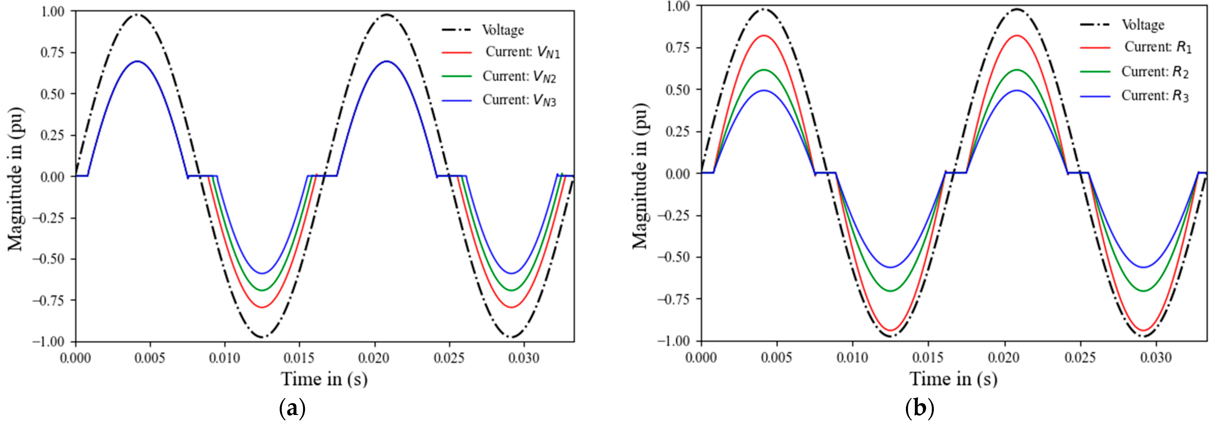
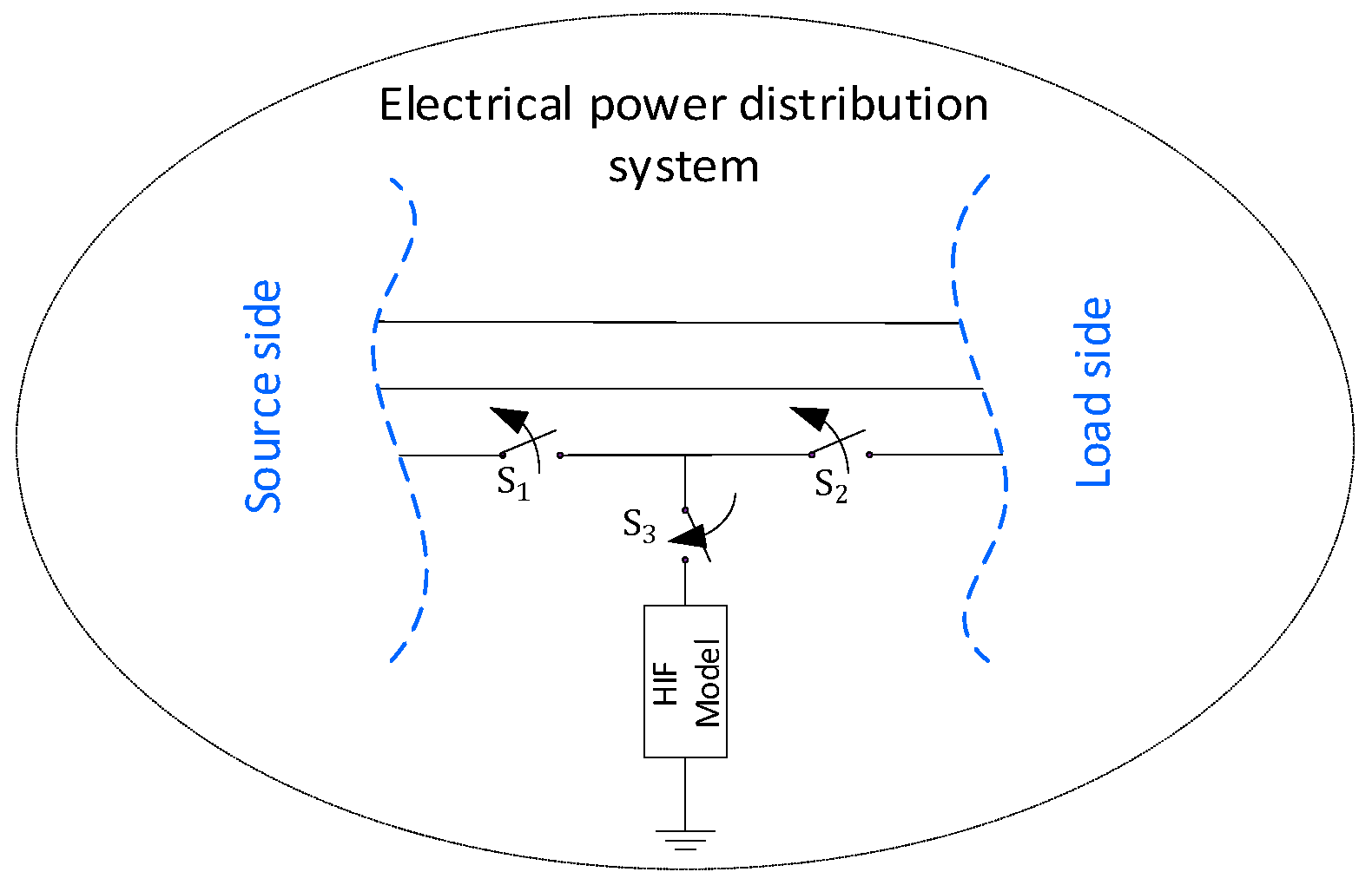
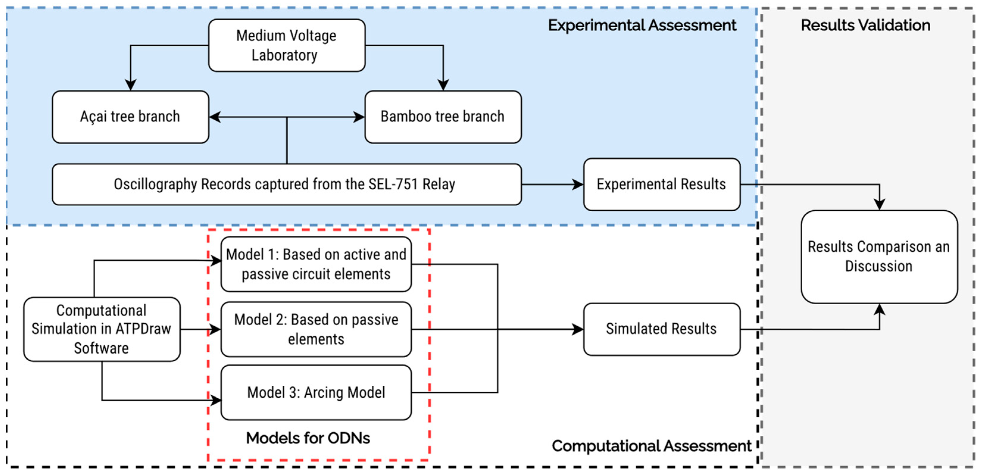
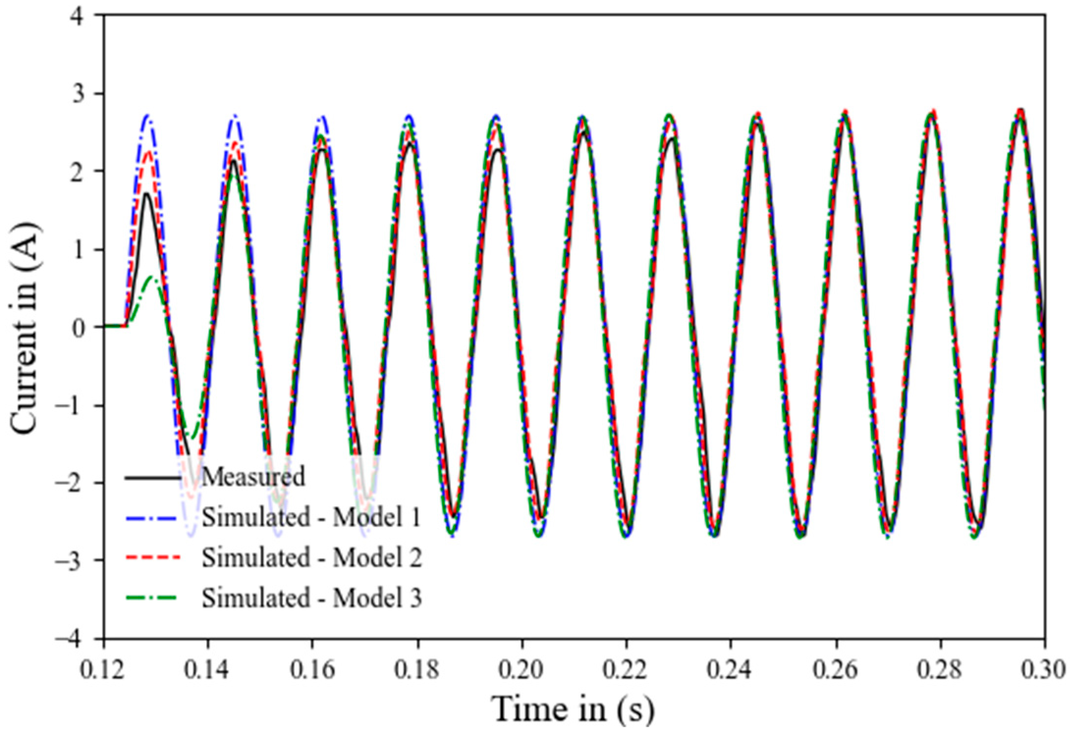
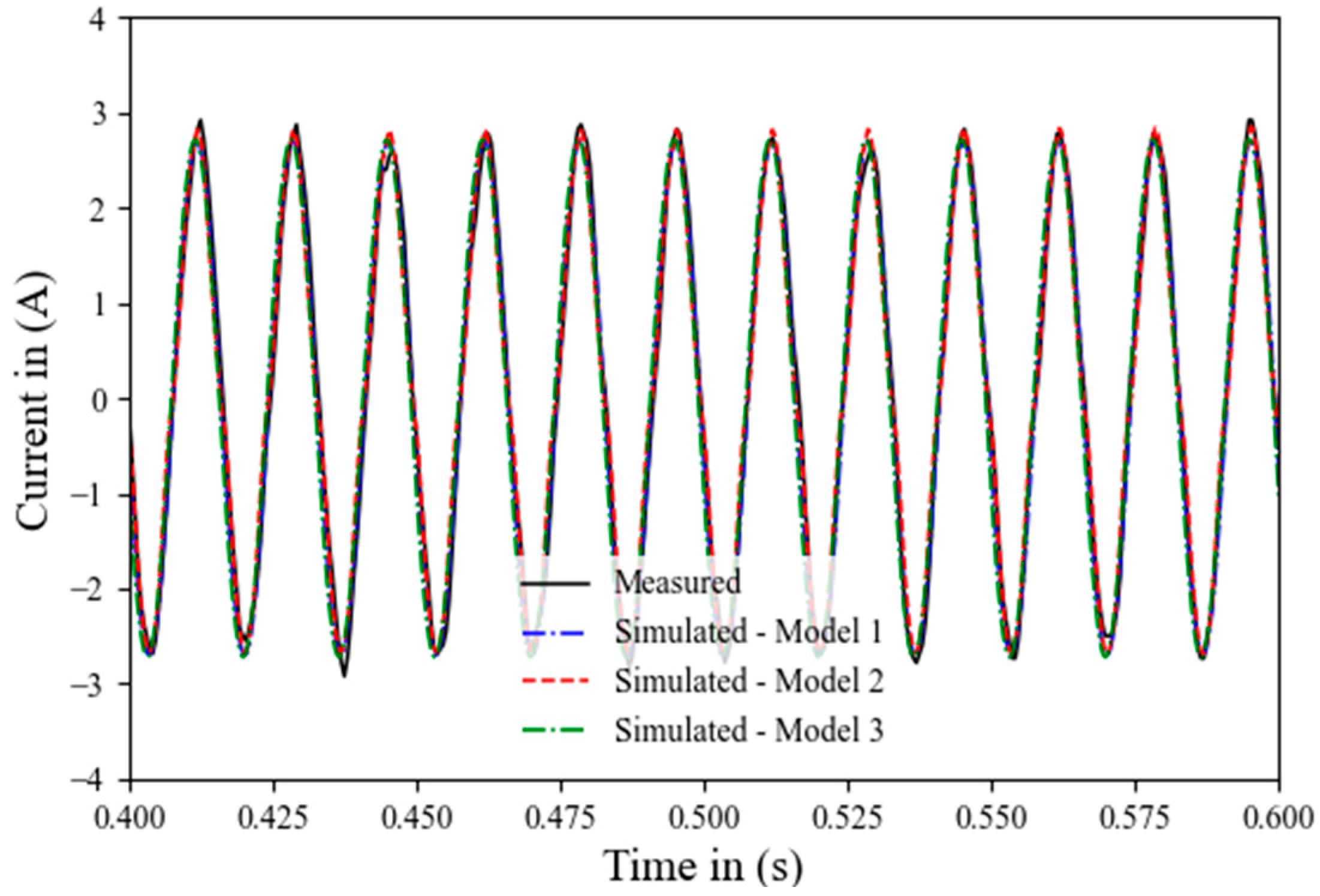
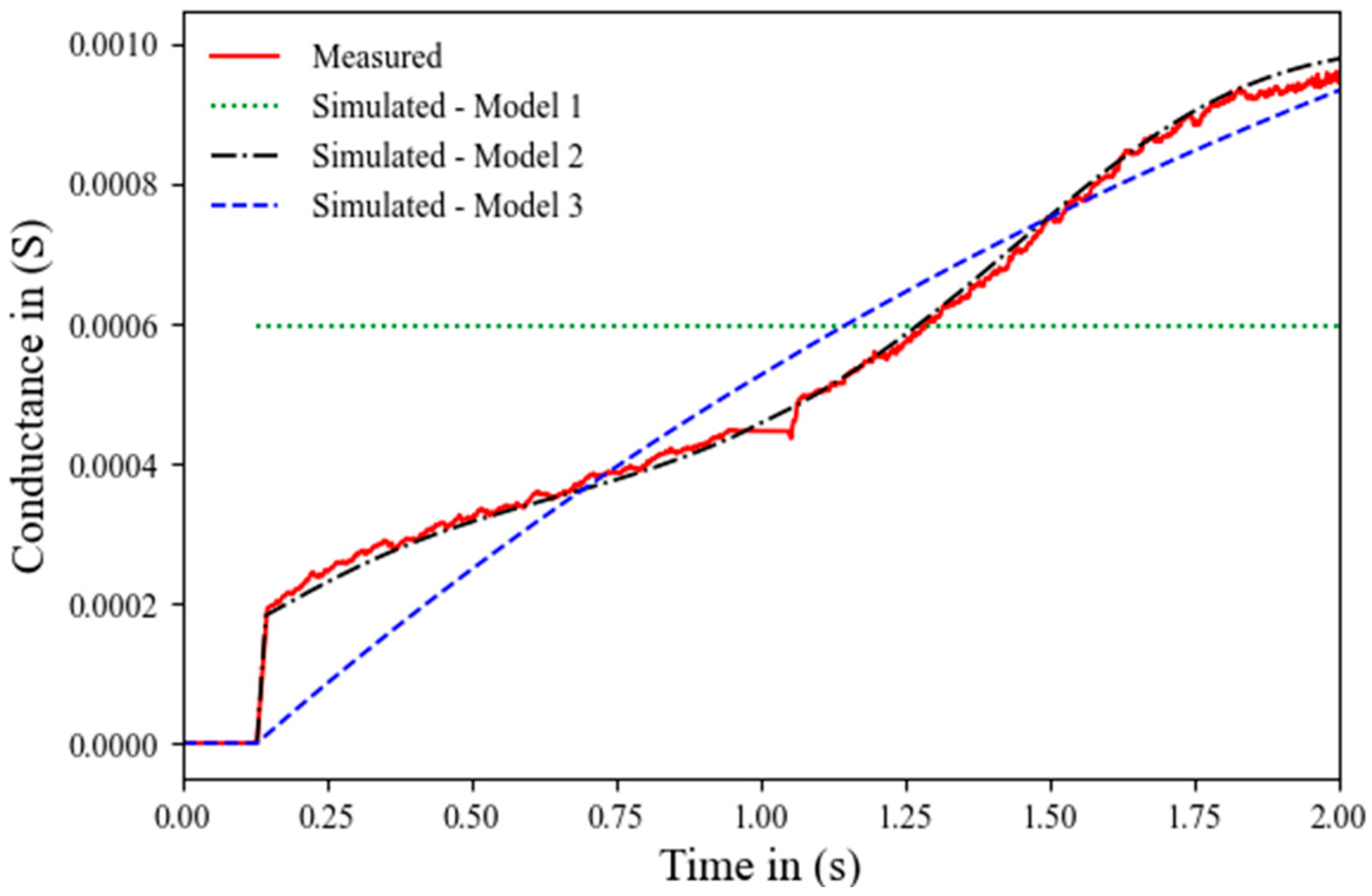
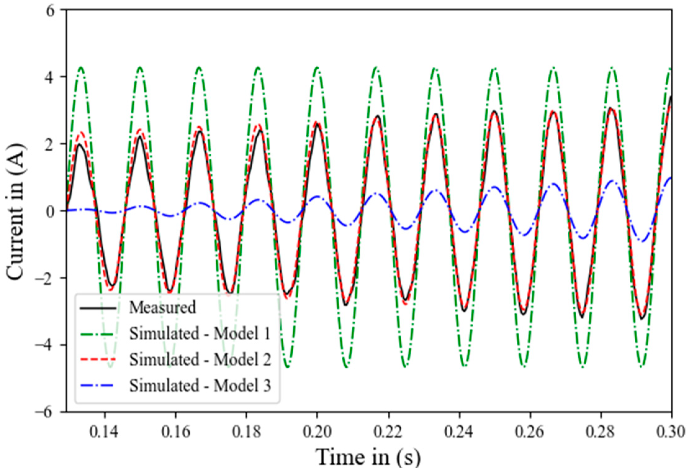
5. Comparison of HIF Models for ODN with MV Lab Test Measured Data

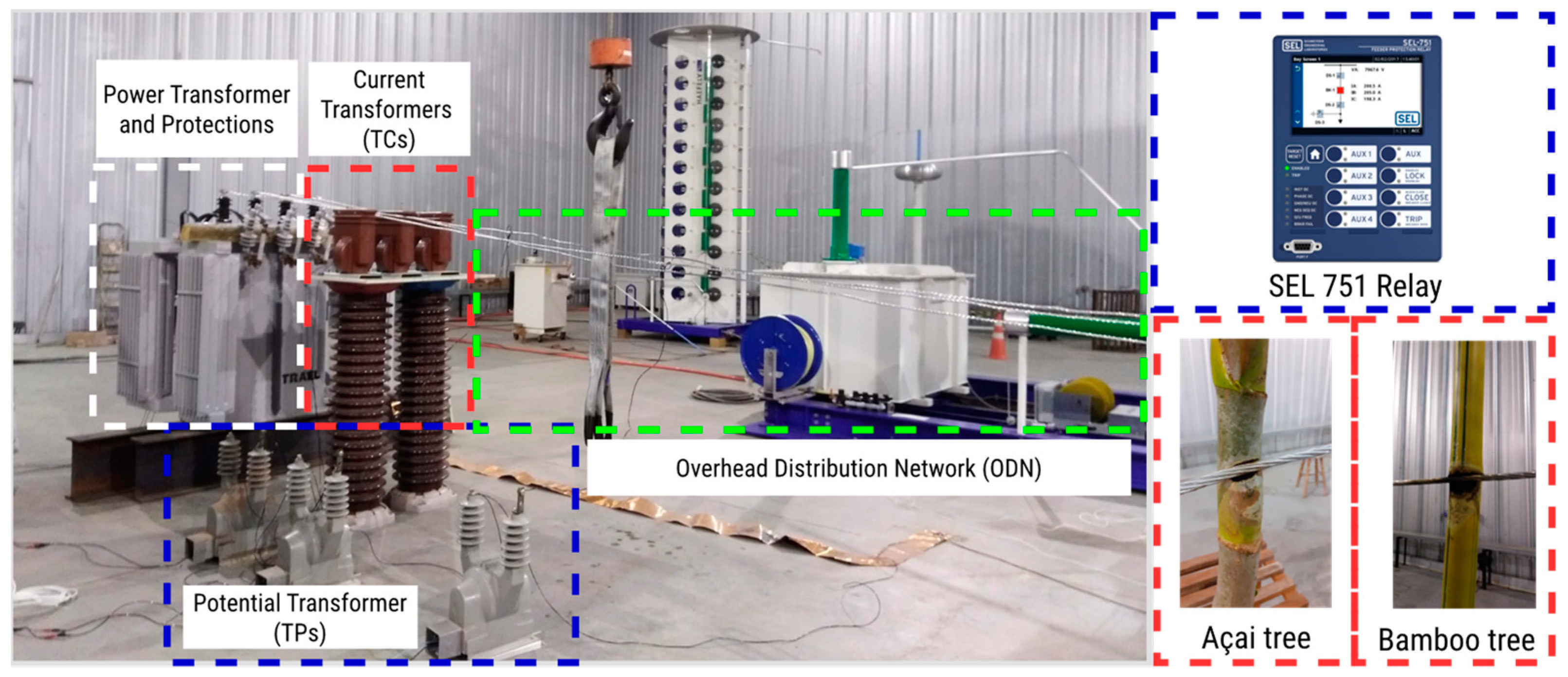
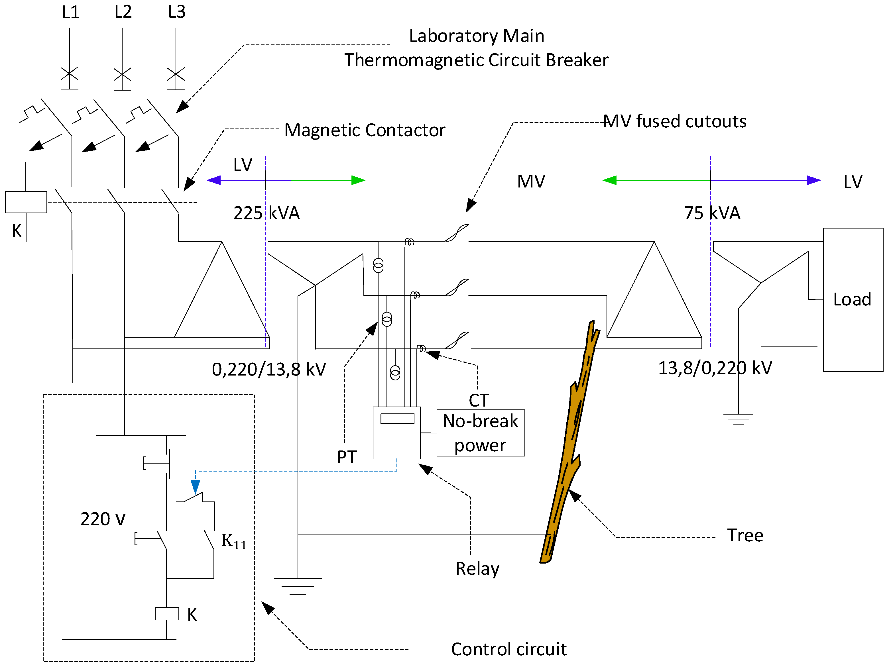
5.1. Materials and Methods

Besides the systematic literature review, this study presents an experimental evaluation to verify the three predominant HIF models with real data obtained from oscillographs in laboratory facilities. Figure 9 shows the methodology used in this study. The computational evaluation was carried out using the ATP/EMTP software (https://atp-emtp.org/, accessed on 25 January 2020) for the simulation of all the HIF models. The following types of HIF models for ODN are compared in this section with lab test results:
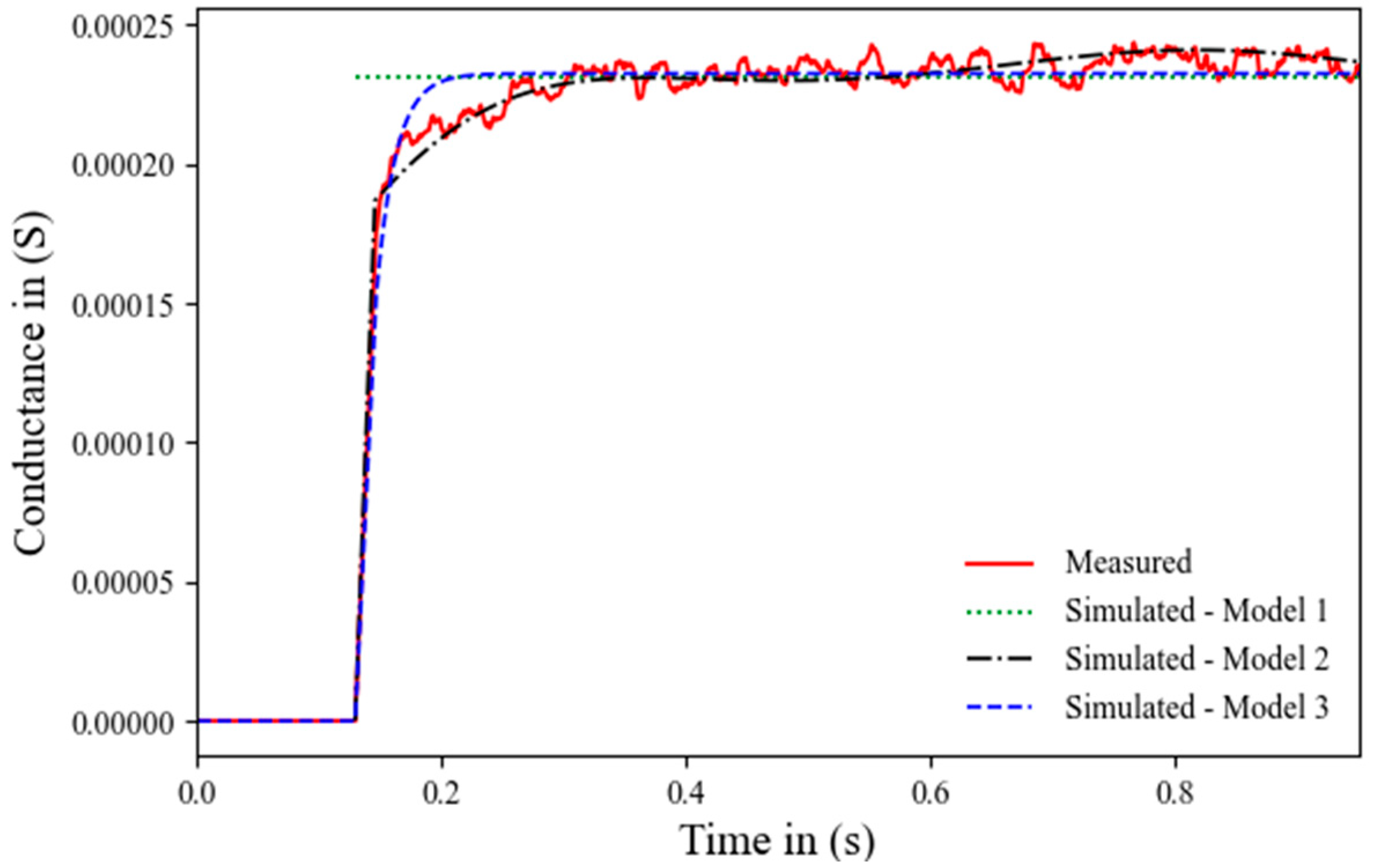
  • Model 1—model based on active and passive circuit elements;
  • Model 2—model based on passive elements;
  • Model 3—arcing model.
For the experimental assessment, the HIF experiments have been carried out at the MV distribution system laboratory or MV lab, Federal University of Para, Brazil. The MV lab was designed and developed for HIF testing purposes. Figure 10 shows the facilities and equipment where the experiments were carried out, and Figure 11 the three-line diagram of the MV laboratory. The MV lab comprises a 225 kVA, 0.22 V/13.8 kV transformer of the WEG manufacturer (Wetherill Park, Australia), SEL-751 feeder protection relay of the SEL manufacturer (Pullman, WA, USA), an alternating current (AC) contactor of the WEG manufacturer, breaker circuits, fuses, potential transformers (PTs), current transformers (CTs), conductors, 75 kVA, 13.8 kV/0.22 kV service transformer of the WEG manufacturer and load.
The 225 kVA transformer is delta connected on the low-voltage (LV) side (0.22 kV) and grounded wye connected on the medium voltage (MV) side (13.8 kV) to emulate a typical distribution substation. The MV system is a three-phase three-wire circuit, and the neutral conductor is grounded on the transformer. In this paper, oscillography records captured by the SEL-751 relay are used to compare the three HIF models. The oscillography records were obtained from two HIF experimental tests, one using a Bamboo tree branch and the other using an Açai tree branch. The SEL-751 relay’s residual overcurrent element was used for tripping purposes with a sensitive setting.

5.2. Results and Discussion

From the measurements in the laboratory presented in Figure 10, data were obtained from the relay for further processing and analysis. Figure 12 and Figure 13 show HIF current waveforms obtained through experimental laboratory tests using a bamboo tree branch and an açai tree branch (common trees in the Amazon region, site of the study), respectively, both subjected to a 13.8/ 3 kV phase voltage. The two waveforms were selected because they present the typical characteristics of a HIF, such as nonlinearity, asymmetry, shoulder and build up, especially because they have a marked envelope, one with an increasing envelope, where the magnitude of the instantaneous current exceeds 10 A, and the other with an oscillating envelope, where the maximum current does not exceed 3 A. To evaluate the limitations or capabilities of the studied models, the two HIF current waveforms are reproduced, using the three selected models. The models are implemented in the ATPDraw software version 7.0, and the results of the simulations are presented graphically, where the differences in the reproduced currents in relation to the measured current can be visually appreciated.
Figure 14 shows the comparison of the conductance reproduced by each type of HIF model with the measured conductance data (red color curve) from an experimental HIF test with a bamboo tree branch. The conductance is determined by the relationship between simulated or measured current and voltage waveforms. When Model 1 is used, the average conductance calculated for positive and negative cycles are 0.00023084 S and 0.00023094 S, respectively.
In this case, they are practically the same, indicating that the asymmetry is negligible. It is noteworthy that the parameters of Model 1 are constant and therefore the conductance is represented by a straight (cyan color line). The black color curve is the conductance calculated using Model 2, represented by a fifth-order polynomial expressed by Equation (6), where its coefficients were determined by fitting the curve. The blue color curve is the conductance calculated using Model 3, whose parameters G 0 = 0.000232432   S and τ = 0.016045   s were estimated by the least-squares method. Note that the conductance calculated using the model 2 has better matching with the measured conductance (red color curve), both in the transient and steady-state conditions. The steady-state condition is reached when t = 0.35 s.
Figure 15 and Figure 16 show comparisons of the current waveforms calculated by HIF models with the measured current waveforms resulting from a HIF experimentally generated by a bamboo tree branch, for transient and steady-state conditions, respectively. The steady-state condition is reached when t = 0.3 s. It can be observed that the Model 2 more accurately replicates the measured transient waveform when compared with Models 1 and 3. As for the steady-state waveform, all HIF models have similar and sufficiently accurate results.
Figure 17 shows the comparison of the conductance reproduced by each type of HIF model with the measured conductance data (red color curve) from an experimental HIF testing with açai tree branch. The average conductance calculated using Model 1 for positive and negative cycles are 0.00059475 S and 0.00059823 S, respectively. The black color curve is the conductance calculated using Model 2 represented by a sixth-order polynomial. The blue color curve is the conductance calculated using Model 3, whose parameters G 0 = 0.001699   S and τ = 2.345621   S were estimated by the least-squares method. It can be observed that model 2 accurately reproduces the measured conductance in the transient and steady-state conditions.
Figure 18 and Figure 19 show comparisons of the current waveforms calculated by HIF models with the measured current waveforms resulting from a HIF experimentally generated by an Açai tree branch, for transient and steady-state conditions, respectively. The steady-state condition is reached when t = 0.35 s. It can be observed that the Model 2 accurately replicates the measured current waveform when compared with Models 1 and 3, for both transient and steady-state conditions.

6. Conclusions

Currently, models based on active and passive circuit elements are the most widely used category in investigations related to the detection and location of HIF. This paper systematically reviewed three broad categories of HIF models for overhead distribution network studies performed by EMT-type programs and compared three well-known HIF models, one of each category, with MV laboratory experimental data. The comparison presented in this work showed that the model based on two non-linear resistances is more accurately matched with measured waveforms obtained from two experimental HIF tests using tree branches when compared with other models. The presented review, models, studies, and comparison will be useful to researchers and practicing distribution protection engineers who are actively using EMT simulation tools for modeling and analysis of overhead distribution networks. The lab experimental results reported in this paper encourage further research to develop new high-impedance fault models using a large database repository of lab experimental tests or actual field events.

Author Contributions

Conceptualization, J.C.H.P. and J.P.A.V.; methodology, A.P.L. and J.C.H.P.; software, M.A.M.C. and J.C.H.P.; validation, J.M.T. and J.C.H.P.; formal analysis, G.C.J., A.P.d.M. and P.E.F.; investigation, J.C.H.P., J.M.T. and A.P.L.; resources, J.P.A.V., G.C.J., A.P.d.M. and P.E.F.; data curation, J.C.H.P., A.P.L. and M.A.M.C.; writing—original draft preparation, J.C.H.P., J.M.T. and J.P.A.V.; writing—review and editing, J.C.H.P., J.M.T., A.P.L. and M.A.M.C.; supervision, J.P.A.V., G.C.J., A.P.d.M. and P.E.F.; funding acquisition, J.P.A.V. All authors have read and agreed to the published version of the manuscript.

Funding

This work was supported by the Energy Equatorial Group at the Research and Development Project Number PD-00371-0039/2019 and the publication taxes by the Pro-Rectory of Research and Post-Graduate Studies-PROPESP/UFPA with call PI O10ACO9403N-PAPQ.

Conflicts of Interest

The authors declare no conflict of interest.

References

  1. Adamiak, M.; Wester, C.; Thakur, M.; Jensen, C. High Impedance Fault Detection on Distribution Feeders. 12p. Available online: https://www.aer.gov.au/system/files/Mr%20Marcus%20Steel%20-%20Attachment%20B%20to%20submission%20on%20Ergon%20Energy%20application%20for%20ring%20fencing%20waiver%20-%20December%202015.pdf (accessed on 3 September 2022).
  2. Ghaderi, A.; Mohammadpour, H.A.; Ginn, H.L.; Shin, Y.-J. High-Impedance Fault Detection in the Distribution Network Using the Time-Frequency-Based Algorithm. IEEE Trans. Power Deliv. 2015, 30, 1260–1268. [Google Scholar] [CrossRef]
  3. Theron, J.C.J.; Pal, A.; Varghese, A. Tutorial on high impedance fault detection. In Proceedings of the 2018 71st Annual Conference for Protective Relay Engineers (CPRE), College Station, TX, USA, 26–29 March 2018; pp. 1–23. [Google Scholar]
  4. Ojanguren, I.; Steynberg, G.; Channelière, J.-L.; Karsenti, L.; Das, R. High Impedance Faults; CIGRE BROCHURE by WG B5.94; CIGRE Publication: Paris, France, 2009. [Google Scholar]
  5. Ghaderi, A.; Ginn, H.L.; Mohammadpour, H.A. High impedance fault detection: A review. Electr. Power Syst. Res. 2017, 143, 376–388. [Google Scholar] [CrossRef]
  6. Balser, S.J.; Clements, K.A.; Kallaur, E. Detection of High Impedance Faults. Available online: http://royalcommission.vic.gov.au/Commission-Reports/Final-Report/Summary.html (accessed on 6 May 2020).
  7. Russell, B.D. Detection of Arcing Faults on Distribution Feeders. Final Report; Research Foundation, Texas A and M University: College Station, TX, US, 1982. [Google Scholar]
  8. Hou, D. Detection of high-impedance faults in power distribution systems. In Proceedings of the 2007 Power Systems Conference: Advanced Metering, Protection, Control, Communication, and Distributed Resources, Clemson, SC, USA, 13–16 March 2007; pp. 85–95. [Google Scholar]
  9. Emanuel, A.E.; Cyganski, D.; Orr, J.A.; Shiller, S.; Gulachenski, E.M. High impedance fault arcing on sandy soil in 15 kV distribution feeders: Contributions to the evaluation of the low frequency spectrum. IEEE Trans. Power Deliv. 1990, 5, 676–686. [Google Scholar] [CrossRef]
  10. Zamanan, N.; Sykulski, J. The evolution of high impedance fault modeling. In Proceedings of the 2014 16th International Conference on Harmonics and Quality of Power (ICHQP), Bucharest, Romania, 25–28 May 2014; pp. 77–81. [Google Scholar]
  11. Nam, S.R.; Park, J.K.; Kang, Y.C.; Kim, T.H. A modeling method of a high impedance fault in a distribution system using two series time-varying resistances in EMTP. In Proceedings of the 2001 Power Engineering Society Summer Meeting, Vancouver, BC, Canada, 15–19 July 2001; Conference Proceedings (Cat. No.01CH37262). Volume 2, pp. 1175–1180. [Google Scholar]
  12. dos Santos, W.C.; de Souza, B.A.; Brito, N.S.D.; Costa, F.B.; Paes, M.R.C. High Impedance Faults: From Field Tests to Modeling. J. Control Autom. Electr. Syst. 2013, 24, 885–896. [Google Scholar] [CrossRef]
  13. Cassie, A.M. Theorie Nouvelle des Arcs de Rupture et de la Rigidité des Circuits; Cigre: Paris, France, 1939; pp. 588–608. [Google Scholar]
  14. Mayr, O. Beiträge zur Theorie des statischen und des dynamischen Lichtbogens. Arch. F. Elektrotechnik 1943, 37, 588–608. [Google Scholar] [CrossRef]
  15. Torres, V.; Guardado, J.L.; Ruiz, H.F.; Maximov, S. Modeling and detection of high impedance faults. Int. J. Electr. Power Energy Syst. 2014, 61, 163–172. [Google Scholar] [CrossRef]
  16. Torres-Garcia, V.; Guillen, D.; Olveres, J.; Escalante-Ramirez, B.; Rodriguez-Rodriguez, J.R. Modelling of high impedance faults in distribution systems and validation based on multiresolution techniques. Comput. Electr. Eng. 2020, 83, 106576. [Google Scholar] [CrossRef]
  17. Lavanya, S.; Prabakaran, S.; Kumar, N.A. Literature Review: High Impedance Fault in Power System and Detection Techniques. Math. Stat. Eng. Appl. 2022, 71, 944–958. [Google Scholar] [CrossRef]
  18. Li, L.; Redfern, M.A. A review of techniques to detect downed conductors in overhead distribution systems. In Proceedings of the 2001 Seventh International Conference on Developments in Power System Protection (IEE), Amsterdam, The Netherland, 9–12 April 2001; pp. 169–172. [Google Scholar]
  19. Aljohani, A.; Habiballah, I. High-Impedance Fault Diagnosis: A Review. Energies 2020, 13, 6447. [Google Scholar] [CrossRef]
  20. Varghese, P.R.; Subathra, M.S.P.; Mathew, C.; George, S.T.; Sairamya, N.J. High Impedance Fault Arc Modeling—A Review. In Intelligent Solutions for Smart Grids and Smart Cities; Siano, P., Williamson, S., Beevi, S., Eds.; Springer Nature: Singapore, 2023; pp. 163–181. [Google Scholar]
  21. Cordeiro, M.A.M.; Heringer, W.R.; Paye, J.C.H.; Sousa, A.L.; Leão, A.P.; Vieira, J.P.A.; Farias, P.E.; Wontroba, A.; Gallas, M.; Rossini, J.P.; et al. Validation of a High Impedance Fault Model for Overhead Distribution Networks Using Real Oscillography Data. In Proceedings of the 13th Latin-American Congress On Electricity Generation and Transmission, Santiago de, Chile, Chile, 20–23 October 2019; FDCT: Irvine, CA, USA, 2019. [Google Scholar]
  22. Elkalashy, N.I.; Lehtonen, M.; Darwish, H.A.; Izzularab, M.A.; Taalab, A.I. Modeling and experimental verification of high impedance arcing fault in medium voltage networks. IEEE Trans. Dielectr. Electr. Insul. 2007, 14, 375–383. [Google Scholar] [CrossRef]
  23. Leão, A.P.; Tostes, M.E.L.; Vieira, J.P.A.; Bezerra, U.H.; Heringer, W.R.; Sousa, A.L.; Cordeiro, M.A.M.; Paye, J.C.H.; Santos, M.C. Characteristics of High Impedance Faults in Overhead Distribution Networks in Bamboo Branches. In Proceedings of the 2020 IEEE PES Transmission & Distribution Conference and Exhibition—Latin America (T&D LA), Montevideo, Uruguay, 28 September–2 October 2020; pp. 1–6. [Google Scholar]
  24. Wontroba, A.; Morais, A.P.; Cardoso, G.J.; Vieira, J.P.A.; Farias, P.E.; Gallas, M.; Rossini, J.P. High-impedance fault detection on downed conductor in overhead distribution networks. Electr. Power Syst. Res. 2022, 211, 108216. [Google Scholar] [CrossRef]
  25. Wontroba, A.; de Morais, A.P.; Rossini, J.P.; Gallas, M.; Cardoso, G.; Vieira, J.P.A.; Farias, P.E.; Santos, M.C. Modeling and Real-Time Simulation of High Impedance Faults for Protection Relay Testing and Methods Validation. In Proceedings of the 2019 IEEE PES Innovative Smart Grid Technologies Conference—Latin America (ISGT Latin America), Gramado, Brazil, 15–18 September 2019; pp. 1–6. [Google Scholar]
  26. Farias, P.E.; de Morais, A.P.; Rossini, J.P.; Cardoso, G. Non-linear high impedance fault distance estimation in power distribution systems: A continually online-trained neural network approach. Electr. Power Syst. Res. 2018, 157, 20–28. [Google Scholar] [CrossRef]
  27. de Sousa, Á.L.; Vieira, J.P.A.; de Melo Cordeiro, M.A.; Leão, A.P.; Paye, J.C.H.; de Morais, A.P.; Junior, G.C.; Santos, M.C. Harmonic Analysis of High-Impedance Fault Experimental Current Waveforms Using Fast Fourier Transform. Simpósio Bras. Sist. Elétricos SBSE 2022, 2, 1958–1965. [Google Scholar] [CrossRef]
  28. Heringer, W.R.; Cordeiro, M.A.M.; Paye, J.C.H.; Sousa, A.L.; Leão, A.P.; Vieira, J.P.A.; Santos, M.C.; Cardoso, G.; de Morais, A.P.; Wontroba, A.; et al. Reproduction of a High Impedance Double line-to-ground Fault Using Real Oscillography Data. In Proceedings of the 2020 IEEE PES Transmission & Distribution Conference and Exhibition—Latin America (T&D LA), Montevideo, Uruguay, 28 September–2 October 2020; pp. 1–6. [Google Scholar]
  29. Aucoin, B.M.; Russell, B.D. Distribution High Impedance Fault Detection Utilizing High Frequency Current Components. IEEE Power Eng. Rev. 1982, PER-2, 46–47. [Google Scholar] [CrossRef]
  30. Jeerings, D.I.; Linders, J.R. Unique aspects of distribution system harmonics due to high impedance ground faults. IEEE Trans. Power Deliv. 1990, 5, 1086–1094. [Google Scholar] [CrossRef]
  31. Trondoli, L.H.P.D.C. Modelo Estocástico Parametrizável Para o Estudo de Faltas de Alta Impedância em Sistemas de Distribuição de Energia Elétrica. Masters’ Thesis, Universidade de São Paulo, São Carlos, Brazil, 2018. [Google Scholar]
  32. Lopes, F.V.; Santos, W.C.; Fernandes, D.; Neves, W.L.A.; Brito, N.S.D.; Souza, B.A. A transient based approach to diagnose high impedance faults on smart distribution networks. In Proceedings of the 2013 IEEE PES Conference on Innovative Smart Grid Technologies (ISGT Latin America), Sao Paulo, Brazil, 15–17 April 2013; pp. 1–8. [Google Scholar]
  33. Santos, W.C.; Costa, F.B.; Silva, J.A.C.B.; Lira, G.R.S.; Souza, B.A.; Brito, N.S.D.; Paes Junior, M.R.C. Automatic building of a simulated high impedance fault database. In Proceedings of the 2010 IEEE/PES Transmission and Distribution Conference and Exposition: Latin America (T D-LA), Sao Paulo, Brazil, 8–10 November 2010; pp. 550–554. [Google Scholar]
  34. Masa, A.V.; Werben, S.; Maun, J.C. Incorporation of data-mining in protection technology for high impedance fault detection. In Proceedings of the 2012 IEEE Power and Energy Society General Meeting, San Diego, CA, USA, 22–26 July 2012; pp. 1–8. [Google Scholar]
  35. Benner, C.L.; Russell, B.D. Practical high-impedance fault detection on distribution feeders. IEEE Trans. Ind. Appl. 1997, 33, 635–640. [Google Scholar] [CrossRef]
  36. Aucoin, B.M.; Jones, R.H. High impedance fault detection implementation issues. IEEE Trans. Power Deliv. 1996, 11, 139–148. [Google Scholar] [CrossRef]
  37. Sultan, A.F.; Swift, G.W.; Fedirchuk, D.J. Detecting arcing downed-wires using fault current flicker and half-cycle asymmetry. IEEE Trans. Power Deliv. 1994, 9, 461–470. [Google Scholar] [CrossRef]
  38. Costa, F.B.; Souza, B.A.; Brito, N.S.D.; Silva, J.A.C.B.; Santos, W.C. Real-Time Detection of Transients Induced by High-Impedance Faults Based on the Boundary Wavelet Transform. IEEE Trans. Ind. Appl. 2015, 51, 5312–5323. [Google Scholar] [CrossRef]
  39. Ramos, M.; Bretas, A.; Bernardon, D.; Pfitscher, L. Distribution networks HIF location: A frequency domain system model and WLS parameter estimation approach. Electr. Power Syst. Res. 2017, 146, 170–176. [Google Scholar] [CrossRef]
  40. Macedo, J.R.; Resende, J.W.; Bissochi, C.A.; Carvalho, D.; Castro, F.C. Proposition of an interharmonic-based methodology for high-impedance fault detection in distribution systems. Transm. Distrib. IET Gener. 2015, 9, 2593–2601. [Google Scholar] [CrossRef]
  41. Russell, B.D.; IEEE Power Engineering Society; Power Engineering Education Committee; Power Systems Relaying Committee; Transmission and Distribution Committee; Substations Committee. IEEE Tutorial Course, Detection of Downed Conductors on Utility Distribution Systems; Publications Sales Department, Institute of Electrical and Electronics Engineers: New York, NY, USA; IEEE Service Center: Piscataway, NJ, USA, 1989. [Google Scholar]
  42. Mangueira Lima, É.; dos Santos Junqueira, C.M.; Silva Dantas Brito, N.; de Souza, B.A.; de Almeida Coelho, R.; Gayoso Meira Suassuna de Medeiros, H. High impedance fault detection method based on the short-time Fourier transform. Transm. Distrib. IET Gener. 2018, 12, 2577–2584. [Google Scholar] [CrossRef]
  43. Sedighi, A.-R.; Haghifam, M.-R.; Malik, O.P.; Ghassemian, M.-H. High impedance fault detection based on wavelet transform and statistical pattern recognition. IEEE Trans. Power Deliv. 2005, 20, 2414–2421. [Google Scholar] [CrossRef]
  44. Sarwar, M.; Mehmood, F.; Abid, M.; Khan, A.Q.; Gul, S.T.; Khan, A.S. High impedance fault detection and isolation in power distribution networks using support vector machines. J. King Saud Univ. Eng. Sci. 2019, 32, 524–535. [Google Scholar] [CrossRef]
  45. Snider, L.A.; Yuen, Y.S. The artificial neural-networks-based relay algorithm for the detection of stochastic high impedance faults. Neurocomputing 1998, 23, 243–254. [Google Scholar] [CrossRef]
  46. Dong, X.; Shi, S. Single Phase to Ground Fault Processing. In Fault Location and Service Restoration for Electrical Distribution Systems; John Wiley & Sons, Ltd.: Hoboken, NJ, USA, 2016; pp. 163–203. ISBN 978-1-118-95028-9. [Google Scholar]
  47. Sharaf, A.M.; Snider, L.A.; Debnath, K. A neural network based relaying scheme for distribution system high impedance fault detection. In Proceedings of the Proceedings 1993 The First New Zealand International Two-Stream Conference on Artificial Neural Networks and Expert Systems, Dunedin, New Zealand, 24–26 November 1993; pp. 321–324. [Google Scholar]
  48. Wai, D.C.T.; Yibin, X. A novel technique for high impedance fault identification. IEEE Trans. Power Deliv. 1998, 13, 738–744. [Google Scholar] [CrossRef]
  49. Sheng, Y.; Rovnyak, S.M. Decision tree-based methodology for high impedance fault detection. IEEE Trans. Power Deliv. 2004, 19, 533–536. [Google Scholar] [CrossRef]
  50. Michalik, M.; Rebizant, W.; Lukowicz, M.; Lee, S.-J.; Kang, S.-H. Wavelet transform approach to high impedance fault detection in MV networks. In Proceedings of the 2005 IEEE Russia Power Tech, St. Petersburg, Russia, 27–30 June 2005; pp. 1–7. [Google Scholar]
  51. Zamanan, N.; Sykulski, J.K. Modelling arcing high impedances faults in relation to the physical processes in the electric arc. WSEAS Trans. Power Syst. 2006, 1, 1507–1512. [Google Scholar]
  52. Sedighi, A.R.; Haghifam, M.R. Simulation of high impedance ground fault in electrical power distribution systems. In Proceedings of the 2010 International Conference on Power System Technology, Hangzhou, China, 24–28 October 2010; pp. 1–7. [Google Scholar]
  53. Baqui, I.; Zamora, I.; Mazón, J.; Buigues, G. High impedance fault detection methodology using wavelet transform and artificial neural networks. Electr. Power Syst. Res. 2011, 81, 1325–1333. [Google Scholar] [CrossRef]
  54. Moravej, Z.; Mortazavi, S.H.; Shahrtash, S.M. DT-CWT based event feature extraction for high impedance faults detection in distribution system. Int. Trans. Electr. Energy Syst. 2015, 25, 3288–3303. [Google Scholar] [CrossRef]
  55. Ferraz, R.G.; Iurinic, L.U.; Filomena, A.D.; Gazzana, D.S.; Bretas, A.S. Arc fault location: A nonlinear time varying fault model and frequency domain parameter estimation approach. Int. J. Electr. Power Energy Syst. 2016, 80, 347–355. [Google Scholar] [CrossRef]
  56. Sharat, A.M.; Snider, L.A.; Debnath, K. A neural network based back error propagation relay algorithm for distribution system high impedance fault detection. In Proceedings of the 1993 2nd International Conference on Advances in Power System Control, Operation and Management, APSCOM-93, Hong Kong, China, 7–10 December 1993; Volume 2, pp. 613–620. [Google Scholar]
  57. Lai, T.M.; Snider, L.A.; Lo, E.; Sutanto, D. High-impedance fault detection using discrete wavelet transform and frequency range and RMS conversion. IEEE Trans. Power Deliv. 2005, 20, 397–407. [Google Scholar] [CrossRef]
  58. Shannon, R.E. Introduction to the art and science of simulation. In Proceedings of the 1998 Winter Simulation Conference, Washington, DC, USA, 13–16 December 1998; Proceedings (Cat. No.98CH36274). Volume 1, pp. 7–14. [Google Scholar]
  59. Samantaray, S.R.; Panigrahi, B.K.; Dash, P.K. High impedance fault detection in power distribution networks using time-frequency transform and probabilistic neural network. Transm. Distrib. IET Gener. 2008, 2, 261–270. [Google Scholar] [CrossRef]
  60. Soheili, A.; Sadeh, J.; Bakhshi, R. Modified FFT based high impedance fault detection technique considering distribution non-linear loads: Simulation and experimental data analysis. Int. J. Electr. Power Energy Syst. 2018, 94, 124–140. [Google Scholar] [CrossRef]
  61. Gautam, S.; Brahma, S.M. Detection of High Impedance Fault in Power Distribution Systems Using Mathematical Morphology. IEEE Trans. Power Syst. 2013, 28, 1226–1234. [Google Scholar] [CrossRef]
  62. Ghaderi, A.; Mohammadpour, H.A.; Ginn, H. High impedance fault detection method efficiency: Simulation vs. real-world data acquisition. In Proceedings of the 2015 IEEE Power and Energy Conference at Illinois (PECI), Champaign, IL, USA, 20–21 February 2015; pp. 1–5. [Google Scholar]
  63. Ghaderi, A.; Mohammadpour, H.A.; Ginn, H. Active fault location in distribution network using time-frequency reflectometry. In Proceedings of the 2015 IEEE Power and Energy Conference at Illinois (PECI), Champaign, IL, USA, 20–21 February 2015; pp. 1–7. [Google Scholar]
  64. Nayak, P.K.; Sarwagya, K.; Biswal, T. A novel high impedance fault detection technique in distribution systems with distributed generators. In Proceedings of the 2016 National Power Systems Conference (NPSC), Bhubaneswar, India, 19–21 December 2016; pp. 1–6. [Google Scholar]
  65. Soheili, A.; Sadeh, J.; Lomei, H.; Muttaqi, K. A new high impedance fault detection scheme: Fourier based approach. In Proceedings of the 2016 IEEE International Conference on Power System Technology (POWERCON), Wollongong, NSW, Australia, 28 September-1 October 2016; pp. 1–6. [Google Scholar]
  66. Kavi, M.; Mishra, Y.; Vilathgamuwa, D.M. Detection and identification of high impedance faults in single wire earth return distribution networks. In Proceedings of the 2016 Australasian Universities Power Engineering Conference (AUPEC), Brisbane, Australia, 25–28 September 2016; pp. 1–6. [Google Scholar]
  67. Kavi, M.; Mishra, Y.; Vilathgamuwa, M.D. High-impedance fault detection and classification in power system distribution networks using morphological fault detector algorithm. Transm. Distrib. IET Gener. 2018, 12, 3699–3710. [Google Scholar] [CrossRef]
  68. Soheili, A.; Sadeh, J. Evidential reasoning based approach to high impedance fault detection in power distribution systems. Transm. Distrib. IET Gener. 2017, 11, 1325–1336. [Google Scholar] [CrossRef]
  69. Sedighi, A.-R. A New Model for High Impedance Fault in Electrical Distribution Systems. Available online: http://www.isroset.org/ (accessed on 9 June 2020).
  70. Hong, Y.-Y.; Huang, W.-S.; Chang, Y.-R.; Lee, Y.-D.; Ouyang, D.-C. Locating high-impedance fault in a smart distribution system using wavelet entropy and hybrid self-organizing mapping network. In Proceedings of the 2017 IEEE PES Innovative Smart Grid Technologies Conference Europe (ISGT-Europe), Torino, Italy, 26–29 September 2017; pp. 1–6. [Google Scholar]
  71. Kizilcay, M.; Pniok, T. Digital simulation of fault arcs in power systems. Eur. Trans. Electr. Power 1991, 1, 55–60. [Google Scholar] [CrossRef]
  72. Nunes, J.U.N.; Bretas, A.S.; Bretas, N.G.; Herrera-Orozco, A.R.; Iurinic, L.U. Distribution systems high impedance fault location: A spectral domain model considering parametric error processing. Int. J. Electr. Power Energy Syst. 2019, 109, 227–241. [Google Scholar] [CrossRef]
  73. Carr, J. Detection of High Impedance Faults on Multi-Grounded Primary Distribution Systems. IEEE Trans. Power Appar. Syst. 1981, PAS-100, 2008–2016. [Google Scholar] [CrossRef]
  74. Sharaf, A.M.; El-Sharkawy, R.M.; Al-Fatih, R.; Al-Ketbi, M. High impedance fault detection on radial distribution and utilization systems. In Proceedings of the 1996 Canadian Conference on Electrical and Computer Engineering, Calgary, AB, Canada, 26–29 May 1996; Volume 2, pp. 1012–1015. [Google Scholar]
  75. Sharaf, A.M.; Abu-Azab, S.I. A smart relaying scheme for high impedance faults in distribution and utilization networks. In Proceedings of the 2000 Canadian Conference on Electrical and Computer Engineering, Quebec City, QC, Canada, 13–16 May 2000; Conference Proceedings. Navigating to a New Era (Cat. No.00TH8492). Volume 2, pp. 740–744. [Google Scholar]
  76. Lee, R.E.; Bishop, M.T. A Comparison of Measured High Impedance Fault Data to Digital Computer Modeling Results. IEEE Trans. Power Appar. Syst. 1985, PAS-104, 2754–2758. [Google Scholar] [CrossRef]
  77. Dasco, A.; Marguet, R.; Raison, B. Fault distance estimation in distribution network for high impedance faults. In Proceedings of the 2015 IEEE Eindhoven PowerTech, Eindhoven, The Netherlands, 29 June-2 July 2015; pp. 1–6. [Google Scholar]
  78. Yu, D.C.; Khan, S.H. An adaptive high and low impedance fault detection method. IEEE Trans. Power Deliv. 1994, 9, 1812–1821. [Google Scholar] [CrossRef]
  79. dos Santos, W.C. Identificação de Faltas de Alta Impedância em Sistemas de Distribuição. Ph.D. Thesis, Universidade Federal De Campina Grande, Campina Grande, Brazil. Available online: http://dspace.sti.ufcg.edu.br:8080/xmlui/handle/riufcg/602 (accessed on 14 January 2023).
  80. Wang, B.; Geng, J.; Dong, X. High-Impedance Fault Detection Based on Nonlinear Voltage–Current Characteristic Profile Identification. IEEE Trans. Smart Grid 2018, 9, 3783–3791. [Google Scholar] [CrossRef]
  81. Darwish, H.A.; Elkalashy, N.I. Universal arc representation using EMTP. IEEE Trans. Power Deliv. 2005, 20, 772–779. [Google Scholar] [CrossRef]
  82. Michalik, M.; Rebizant, W.; Lukowicz, M.; Lee, S.-J.; Kang, S.-H. High-impedance fault detection in distribution networks with use of wavelet-based algorithm. IEEE Trans. Power Deliv. 2006, 21, 1793–1802. [Google Scholar] [CrossRef]
  83. Cui, T.; Dong, X.; Bo, Z.; Richards, S. Integrated scheme for high impedance fault detection in MV distribution system. In Proceedings of the 2008 IEEE/PES Transmission and Distribution Conference and Exposition: Latin America, Bogota, Columbia, 13–15 August 2008; pp. 1–6. [Google Scholar]
  84. Cui, T.; Dong, X.; Bo, Z.; Klimek, A.; Edwards, A. Modeling study for high impedance fault detection in MV distribution system. In Proceedings of the 2008 43rd International Universities Power Engineering Conference, Padova, Italy, 1–4 September 2008; pp. 1–5. [Google Scholar]
  85. Torres, V.; Maximov, S.; Ruiz, H.F.; Guardado, J.L. Distributed Parameters Model for High-impedance Fault Detection and Localization in Transmission Lines. Electr. Power Compon. Syst. 2013, 41, 1311–1333. [Google Scholar] [CrossRef]
  86. Torres, V.; Ruiz, H.F.; Maximov, S.; Ramírez, S. Modeling of high impedance faults in electric distribution systems. In Proceedings of the 2014 IEEE International Autumn Meeting on Power, Electronics and Computing (ROPEC), Ixtapa, Mexico, 5–7 November 2014; pp. 1–6. [Google Scholar]
  87. Thomas, M.S.; Bhaskar, N.; Prakash, A. Voltage Based Detection Method for High Impedance Fault in a Distribution System. J. Inst. Eng. India Ser. B 2016, 97, 413–423. [Google Scholar] [CrossRef]
  88. Iurinic, L.U.; Herrera-Orozco, A.R.; Ferraz, R.G.; Bretas, A.S. Distribution Systems High-Impedance Fault Location: A Parameter Estimation Approach. IEEE Trans. Power Deliv. 2016, 31, 1806–1814. [Google Scholar] [CrossRef]
Figure 1. Typical HIF current waveform.
Energies 17 01125 g001
Figure 2. Representation of HIF models based on active and passive circuit elements according to Table 1.
Energies 17 01125 g002
Figure 3. High impedance fault current waveforms: (a) when source voltage varies; (b) when resistance varies.
Energies 17 01125 g003
Figure 4. High impedance fault current and voltage waveforms.
Energies 17 01125 g004
Figure 5. Representation of high impedance fault models based on passive circuit elements according to Table 2.
Energies 17 01125 g005
Figure 6. Representation of high-impedance fault models based on the physical process involved in the electric arc, according to Table 3.
Energies 17 01125 g006
Figure 7. Interaction between the HIF model and distribution network model.
Energies 17 01125 g007
Figure 8. High impedance fault models: (a) based on active and passive circuit elements; (b) based on passive circuit elements.
Energies 17 01125 g008
Figure 9. Flowchart of the methodology proposed for the model validation.
Energies 17 01125 g009
Figure 10. Medium voltage laboratory for the HI testing.
Energies 17 01125 g010
Figure 11. Three-line diagram of the MV lab for HIF testing.
Energies 17 01125 g011
Figure 12. Measured current waveform obtained from a HIF experimental test with a Bamboo tree branch.
Energies 17 01125 g012
Figure 13. Measured current waveform obtained from a HIF experimental test with an Açai tree branch.
Energies 17 01125 g013
Figure 14. Comparison of the conductance reproduced by each type of HIF model with the measured conductance data from a HIF experimental test with a bamboo tree branch.
Energies 17 01125 g014
Figure 15. Comparison of the simulated current waveforms (transient state) with the measured current waveform resulting from an experimental test with a bamboo tree branch.
Energies 17 01125 g015
Figure 16. Comparison of the simulated current waveforms (steady-state condition) with the measured current waveform resulting from an experimental test with a bamboo tree branch.
Energies 17 01125 g016
Figure 17. Comparison of the conductance reproduced by each type of HIF model with the measured conductance data from an HIF experimental test with the Açai tree branch.
Energies 17 01125 g017
Figure 18. Comparison of the simulated current waveforms (transient state) with the measured current waveform resulting from an experimental test with an Açai tree branch.
Energies 17 01125 g018
Figure 19. Comparison of the simulated current waveforms (steady-state condition) with the measured current waveform resulting from an experimental test with an Açai tree branch.
Energies 17 01125 g019
Table 1. Timeline of HID models based on active and passive circuit elements.
ModelYearRef.Element 1Element 2Element 3Element 4Control System
a1990[9]Energies 17 01125 i001Energies 17 01125 i002--Energies 17 01125 i007Energies 17 01125 i008--Energies 17 01125 i005Energies 17 01125 i003- - -
b1993[47]Energies 17 01125 i001Energies 17 01125 i003Energies 17 01125 i002-Energies 17 01125 i007Energies 17 01125 i003Energies 17 01125 i008-Energies 17 01125 i009-- - -
c1998[48]Energies 17 01125 i001Energies 17 01125 i004--Energies 17 01125 i007Energies 17 01125 i004--Energies 17 01125 i009Energies 17 01125 i009Energies 17 01125 i010 Energies 17 01125 i009 TACS
d2004[49]Energies 17 01125 i001Energies 17 01125 i002--Energies 17 01125 i007Energies 17 01125 i008--Energies 17 01125 i009Energies 17 01125 i010- - -
e2005[50]Energies 17 01125 i001Energies 17 01125 i002Energies 17 01125 i006-Energies 17 01125 i007Energies 17 01125 i008Energies 17 01125 i006-Energies 17 01125 i003Energies 17 01125 i010- - MODELS
f2006[51]Energies 17 01125 i001Energies 17 01125 i005Energies 17 01125 i003Energies 17 01125 i002Energies 17 01125 i007Energies 17 01125 i005Energies 17 01125 i003Energies 17 01125 i008--- - -
g2010[52]Energies 17 01125 i001Energies 17 01125 i003Energies 17 01125 i002-Energies 17 01125 i007Energies 17 01125 i003Energies 17 01125 i008-Energies 17 01125 i009-- - -
h2011[53]Energies 17 01125 i001Energies 17 01125 i003Energies 17 01125 i004-Energies 17 01125 i007Energies 17 01125 i003Energies 17 01125 i004-Energies 17 01125 i010-- - -
i2015[54]Energies 17 01125 i001Energies 17 01125 i003Energies 17 01125 i002-Energies 17 01125 i007Energies 17 01125 i003Energies 17 01125 i008-Energies 17 01125 i009Energies 17 01125 i010- - -
j2016[55]Energies 17 01125 i001Energies 17 01125 i002--Energies 17 01125 i007Energies 17 01125 i008--Energies 17 01125 i005Energies 17 01125 i010- - -
k2017[31]Energies 17 01125 i001Energies 17 01125 i002--Energies 17 01125 i007Energies 17 01125 i008--Energies 17 01125 i009Energies 17 01125 i010- Energies 17 01125 i009 MODELS TACS
Table 2. High impedance fault models based on passive circuit elements.
ModelYearRef.Element 1Control System
a1981[73]Energies 17 01125 i010Energies 17 01125 i010-
b1996[74]Energies 17 01125 i011Energies 17 01125 i010-
c1998[46]Energies 17 01125 i009Energies 17 01125 i010MODELS
d2000[75]Energies 17 01125 i005Energies 17 01125 i010-
e2001[11]Energies 17 01125 i010Energies 17 01125 i010TACS
Table 3. High impedance fault models based on the physical process involved in the electric arc.
ModelYearRef.Element 1Control System
a2006[82]Energies 17 01125 i009Energies 17 01125 i010-MODELS
b2007[21]Energies 17 01125 i009Energies 17 01125 i003Energies 17 01125 i010MODELS
c2008[83]Energies 17 01125 i010Energies 17 01125 i010-MODELS
Disclaimer/Publisher’s Note: The statements, opinions and data contained in all publications are solely those of the individual author(s) and contributor(s) and not of MDPI and/or the editor(s). MDPI and/or the editor(s) disclaim responsibility for any injury to people or property resulting from any ideas, methods, instructions or products referred to in the content.

