
Bidding Strategy for Wind and Thermal Power Joint Participation in the Electricity Spot Market Considering Uncertainty
School of Electric Power Engineering, South China University of Technology, Guangzhou 510640, China
*
Author to whom correspondence should be addressed.
Energies 2024, 17(7), 1714; https://0-doi-org.brum.beds.ac.uk/10.3390/en17071714
Submission received: 11 March 2024
/
Revised: 24 March 2024
/
Accepted: 27 March 2024
/
Published: 3 April 2024
(This article belongs to the Special Issue Application of Intelligent Techniques in Power System Stability, Control and Protection)
Abstract
:As the proportion of new energy sources, such as wind power, in the electricity system rapidly increases, their participation in spot market competition has become an inevitable trend. However, the uncertainty of clearing price and wind power output will lead to bidding deviation and bring revenue risks. In response to this, a bidding strategy is proposed for wind farms to participate in the spot market jointly with carbon capture power plants (CCPP) that have flexible regulation capabilities. First, a two-stage decision model is constructed in the day-ahead market and real-time balancing market. Under the joint bidding mode, CCPP can help alleviate wind power output deviations, thereby reducing real-time imbalanced power settlement. On this basis, a tiered carbon trading mechanism is introduced to optimize day-ahead bidding, aiming at maximizing revenue in both the electricity spot market and carbon trading market. Secondly, conditional value at risk (CVaR) is introduced to quantitatively assess the risks posed by uncertainties in the two-stage decision model, and the risk aversion coefficient is used to represent the decision-maker’s risk preference, providing corresponding strategies. The model is transformed into a mixed-integer linear programming model using piecewise linearization and McCormick enveloping. Finally, the effectiveness of the proposed model and methods is verified through numerical examples.
1. Introduction
In the context of developing a low-carbon economy, augmenting the integration of renewable energy into the power system and decarbonizing traditional fossil energy (e.g., coal and oil) are important means to achieve the goals of carbon emission reduction and carbon neutrality as scheduled [1]. With the accelerated construction and development of the electricity spot market, China’s renewable energy sector has essentially shifted from the initial support phase involving benchmark electricity prices and preferential subsidies to a subsidy-free grid-connection phase at parity [2]. The generation capacity of renewable energy sources, including wind and photovoltaic, has experienced consistent growth. Nevertheless, they are no longer afforded the comprehensive grid-connection protection facilitated by the power grid; instead, they engage in competition within the electricity spot market alongside conventional power sources.
The strong randomness and volatility of wind power output make it difficult to accurately predict [3]. The participation of wind power in the spot market not only poses challenges to the secure operation of the power system but also results in penalties for wind power producers arising from the imbalances between the actual output and the winning bid [4]. This significantly weakens the profitability of wind power companies, which is not conducive to the enthusiasm for subsidy-free bidding and the healthy development of new energy. By optimizing resource allocation in the market [5], the combination of wind power with thermal power, energy storage systems, pumped storage power stations, and other types of flexible resources enables energy complementation. As a result, this method efficiently alleviates the anticipated revenue losses arising from deviation penalties, as referenced in [6,7,8]. For the electricity market, this approach is beneficial for solving the problem of insufficient grid reserves, ensuring a continuous and reliable power supply, thereby alleviating the pressure on grid dispatching. Ref. [9] discussed the participation of “new energy + storage” power plants as independent entities in the day-ahead market by controlling the charging and discharging behavior of the storage system to optimize the plant’s power output. Ref. [10] considered the strong uncertainty of wind power output and formulated a bidding strategy for the wind-storage system in the energy market and the frequency regulation auxiliary service market, also taking into account the cycle life cost of storage. Ref. [11] designed a data-driven classification aggregation method for electric vehicles and proposed a day-ahead bidding strategy for the joint participation of electric vehicle fleets and wind power in the electricity and frequency regulation markets. Ref. [12] conducted joint bidding with demand response aggregators and wind power companies, introducing a balancing coefficient to balance the interests of multiple entities. In the above literature, wind power and new market entities such as energy storage collaborate to reduce upper and lower deviations. However, as the installed capacity of new energy continues to increase, there is still an issue with the insufficient scale of storage allocation due to high investment costs.
As traditional market entities, hydroelectric and thermal power possess excellent controllability, enabling them to meet the flexibility demands of integrating large-scale wind power into the grid within a short timeframe. Moreover, the collaborative participation in the market of these traditional market entities alongside wind farms also contributes to enhancing the stability of the electricity market. Ref. [13] investigated the bidding strategy of a coalition of multiple wind farms and pumped storage power stations, using the Shapley value and core solution to address revenue allocation among wind-pumped storage power stations and multiple wind farms. Hydropower is characterized by its sustainability and efficiency, but it entails significant construction costs and resource demands. Furthermore, the establishment of hydropower stations is constrained by geographical conditions. Currently, in China’s “Three Norths” area, where wind power is developed intensively, the power source structure is still dominated by thermal power units and the wind–thermal bundling approach is applied to promote the grid connection of large-capacity wind farms. Therefore, encouraging thermal power companies and new energy companies to carry out substantive joint operations is an effective solution to promote the high-quality development of new energy. In [14,15,16], thermal power units were leveraged to offset stochastic wind power output, demonstrating that the joint bidding strategy can effectively increase the bidding profits for both parties. Ref. [14] proposed a dual-objective bidding strategy for wind–thermal–photovoltaic systems in the electricity and spinning reserve markets. Ref. [15] established a multi-objective, three-stage bidding and scheduling model for maximizing profits and minimizing carbon emissions of a wind–thermal–storage system based on mixed-integer programming. In [16], a wind–thermal joint bidding model was established utilizing the traditional information-gap decision theory method, with the cogeneration units supplying reserved capacity to minimize real-time imbalances. However, traditional thermal power units have a slow ramping rate, resulting in significant costs due to frequent starts and stops for offering adjustment services, and their high carbon emissions are contrary to China’s current “dual carbon” targets.
In the context described above, this paper studies the joint bidding strategy for wind farms and CCPP in the spot market, taking into account imbalance costs. The transformation of traditional thermal power plants into CCPP not only results in lower carbon emission intensity but also provides a wider operating range and faster ramping rate [17], enhancing the environmental, efficiency, and flexibility levels of thermal power units. Consequently, it can serve as an ideal low-carbon power source to implement joint bidding with wind power. On this basis, a tiered carbon trading mechanism is introduced to reduce carbon emissions from thermal power units to achieve the maximum economic benefits in both electricity and carbon markets. The conditional value at risk (CVaR) is introduced to quantify various uncertainties, allowing decision-makers to set an appropriate risk aversion coefficient according to their risk tolerance, thus coordinating profit and risk optimization. Finally, the effectiveness of the proposed model is verified through numerical examples.
2. Theory and Methods
2.1. Mechanism Analysis of Flexible Operation of CCPP
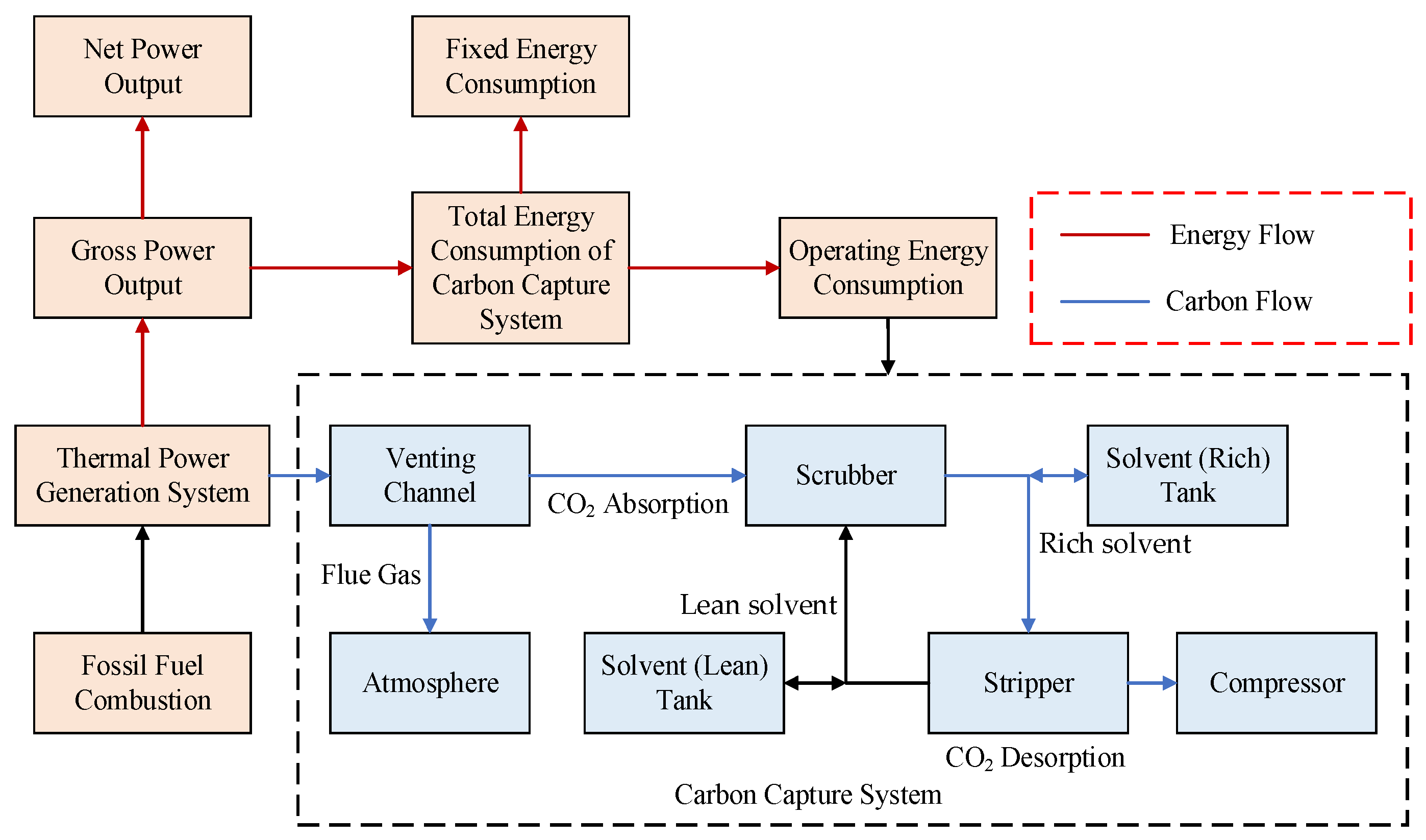
Post-combustion carbon capture technology separates CO2 directly from the flue gas produced by fuel combustion in boilers, capturing it through three stages: absorption, desorption, and compression. This technology has reached a mature state and is widely applied [18]. However, there is a coupling issue between the scrubber and the stripper in CCPP. Specifically, when the ratio of flue gas entering the scrubber from the venting channel to that directly discharged into the atmosphere remains constant, the CCPP cannot independently adjust the energy distribution of the carbon capture facilities. The sole available control option is the adjustment of power output in the CCPP. This results in conflicts between the loads of the generation system and the carbon capture system, posing a challenge for CCPP to harmonize the relationship between carbon capture energy consumption and net power output.
To address these challenges, this paper introduces an integrated, flexible operating mode for CCPP. The carbon flow and energy flow within a CCPP are shown in Figure 1.
This mode introduces two solvent storage tanks between the scrubber and the stripper, disrupting the traditional balance of solvent volumes within each. Firstly, the proportion of flue gas passing through the scrubber can be adjustable by the venting channel. The CO2-containing flue gas has intimate contact with liquid absorbent within the scrubber. Meanwhile, CO2 is absorbed by the MEA (monoethanolamine) solvent. Subsequently, the “rich” solvent, containing a higher concentration of CO2, is directed to the stripper, where it desorbs the CO2 and regenerates the “lean” solvent. A significant amount of thermal energy is required during the regeneration of the solvent during this process. The “lean” solvent is then recirculated back to the scrubber for the next absorption cycle, ensuring a strictly equal bidirectional flow of solvent between the scrubber and the stripper. During the above process, the “rich” solvent storage tank can store the “rich” solvent from the scrubber and pump it to the stripper for further processing when needed. By introducing these auxiliary facilities and decoupling the loads of power generation and carbon capture facilities, the CCPP is able to control the volume of CO2 captured, thus giving the CCPP the opportunity to be operated flexibly [19].
The formula for calculating the mass of CO2 captured by the carbon capture system is generally represented as follows:
where EG,t represents the carbon emissions of the thermal power unit before being captured at hour t. η stands for the carbon capture efficiency. γt denotes the proportion of flue gas entering the scrubber through the venting channel at hour t. BG is the carbon emission coefficient of the thermal power unit, representing the CO2 emission intensity per unit of gross power output. EH,t is the mass of CO2 released by the “rich” solvent storage tank at hour t, with CO2 mass related to the solvent volume as follows:
where df,t represents the volume of “rich” solvent pumped out from the “rich” solvent storage tank at hour t. MMEA is the molar mass of the MEA solution. is the molar mass of CO2. Ε is the quantity of desorption in the stripper. ρf and σf, respectively, denote MEA solvent concentration and density.
The gross power output of the generation system equals the sum of the net power output and the power consumed by the carbon capture system. When the gross power output is fixed, an increase in power consumption by the carbon capture system leads to a decrease in the net power output. This enhances the spinning reserve capacity of the thermal power unit, ensuring greater flexibility and reliability. Under the integrated, flexible operation mode, the solvent storage tank can provide additional CO2. This allows the carbon capture facilities to capture more CO2, resulting in increased capture energy consumption. As a result, the thermal power unit is capable of achieving a significant reduction in its net power output, enabling the CCPP to possess an extended range for net output adjustment.
Compared to conventional coal-fired power units, where the generation cycle is limited by their large thermal inertia and boiler state changes require significant time, the carbon capture facilities in post-combustion CCPP operate downstream of the generation system, providing greater independence. This independence allows for direct adjustment of the energy supply to the carbon capture system, enabling rapid adjustments to the net power output. Additionally, it can store CO2, which is not to be treated in the stripper, so the thermal power unit can provide more power for the load during the peak load period. The carbon capture power plant can realize “energy time shifting” by adjusting the solvent storage, effectively resolving the contradiction between power generation and carbon capture.
2.2. Joint Bidding Strategy for Wind Farms and CCPPs
The generation alliance of wind and thermal power makes bidding decisions at two stages: the day-ahead market and the real-time balancing market. The day-ahead market bid is based on disclosed market information, generation cost functions, forecasted market clearing price, and wind power output. In the first stage, the day before the operation, the generation alliance submits its offering curve that aligns its economic interests to the electricity trading institution. In the MCP (market clearing price) mechanism, the settlement of all the winning generators is based on the unified clearing price λ. Since the capacity of the generation alliance only accounts for a small ratio in the whole market transaction, it is not a determinant of the market clearing price. Its bidding behavior exerts minimal impact on the system’s marginal electricity price. Therefore, this paper assumes that the generation alliance acts as a price taker in the market. Thus, it only needs to submit power bid quantities instead of bidding curves to the market. In the second stage, the power generation plan formulated in the day-ahead market is put into action. Given the existence of forecasting errors, the CCPP performs rapid and precise control of real-time power output on an operational day, ensuring that the actual generation quantities align closely with the scheduled quantities in the day-ahead plan. When the actual electricity deviation of the wind farm surpasses the adjustment capability of the CCPP, the generation alliance enters the real-time balancing market. The imbalance price is used for the settlement of imbalanced electricity, which involves shortages or surpluses of electricity in real time.
Currently, the spot market mechanism in China is not yet mature. To prevent speculators from exploiting the arbitrage between day-ahead and real-time price differences, a dual-pricing mode is adopted in the real-time balancing market to incentivize participants to enhance their forecasting capabilities and provide reliable electricity supply [13]. The penalty coefficients meet the following conditions:
where πdown and πup, respectively, represent the penalty coefficients for positive and negative imbalances. represents the day-ahead market clearing price. and represent the positive and negative imbalance prices, respectively.
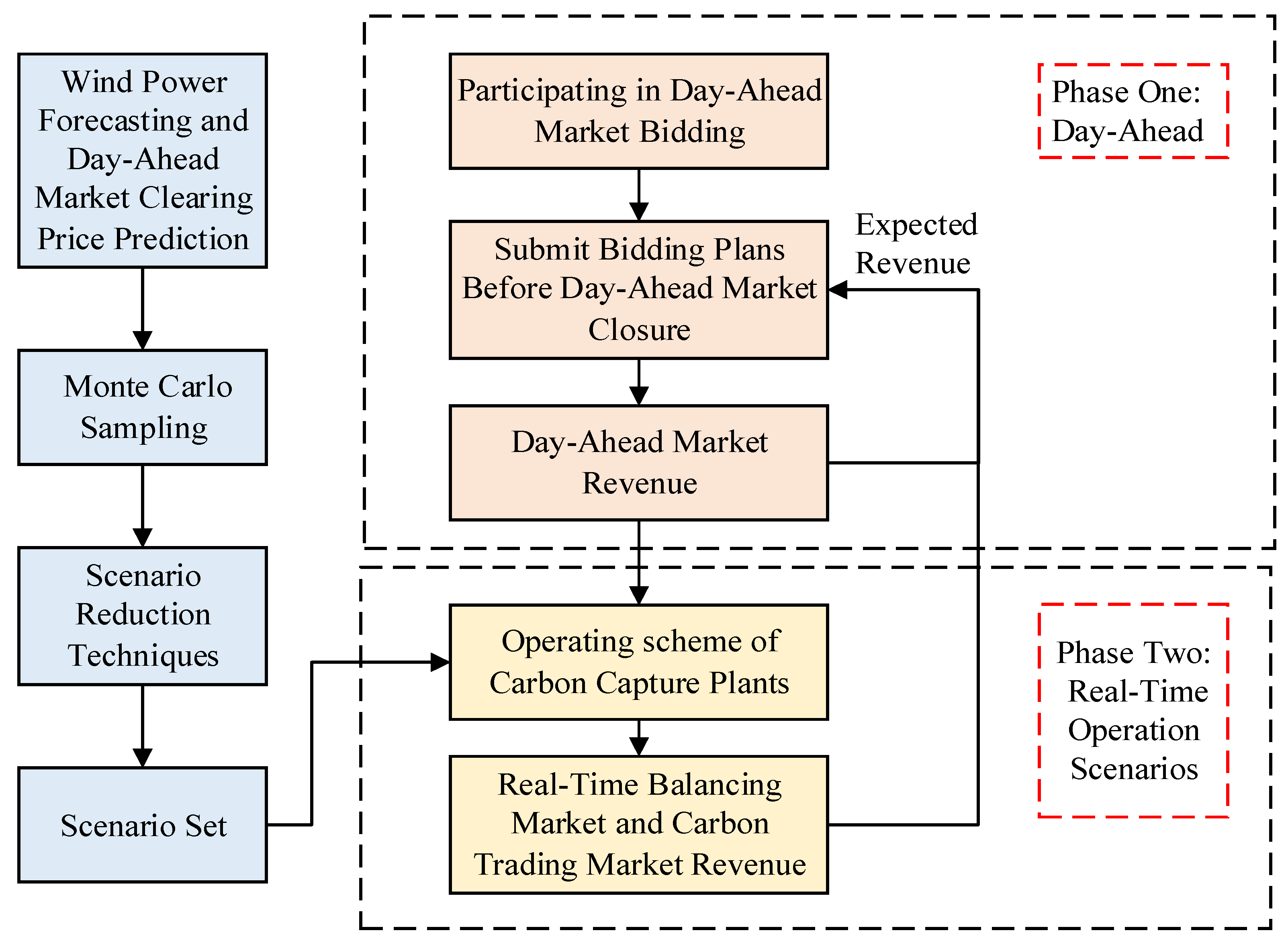
The two-stage decision-making framework is illustrated in Figure 2; the uncertainties of clearing prices and wind power output are modeled via a set of scenarios. Assume that the forecast errors of random variables follow a normal distribution, and the scenarios are generated via random sampling from the probability distribution. Subsequently, a Kantorovich distance-based scenario reduction technique is utilized to establish a set of typical scenarios and their corresponding probabilities. The bidding strategy aims to maximize expected profits and minimize risk as multi-objectives. The risk aversion coefficient is determined based on the risk tolerance levels of generators. The optimal solution is calculated by combining all scenarios along with their respective probabilities. The wind power uncertainty is described through scenarios where the CCPP adjusts its actual net power output based on wind power variations within each scenario.
2.3. Conditional Value at Risk
Should the day-ahead forecast results deviate significantly from the actual values, it can lead to a significant divergence between actual and expected profits. To mitigate the adverse impact of risks on the bidding model, CVaR is utilized as a risk measurement indicator to assess risk, thereby bolstering the robustness of the model. Unlike value at risk (VaR), which focuses on estimating the maximum potential loss within a confidence level, CVaR considers the expected value of losses that exceed the VaR threshold.
The loss function f (x,y) is related to the decision vector and uncertain vector. Here, x represents the decision variables, and y denotes the random variables associated with risk factors. When the joint probability density function p(y) of y is known, the conditional value at risk function under continuous distribution can be formulated as follows:
where β is the confidence level. zβ represents the VaR value at confidence level β. ψ(x,α) denotes the probability that f (x,y) does not exceed the threshold z. Fβ(x) is the expected value of f (x,y) exceeding the VaR.
To address the integral problem, we can utilize a set of sampled scenarios to obtain an equivalent calculation formula for CvaR under discrete distribution as follows:
where N is the total number of sampled scenarios. Φs is the probability of the scenario s.
CVaR is often used as a risk measure for cost-based loss functions. A smaller CVaR implies a lower level of tail cost, indicating a relatively better risk profile. For benefit-based functions, the loss function could be defined as the portion where actual benefits fall below expected benefits [20]. For ease of calculation, this paper defines CVaR as the average benefit when the outcome falls beyond a specified confidence level. CVaR provides a measure of the expected benefit in extreme adverse scenarios, focusing solely on the tail of the distribution beyond the chosen confidence level. The formula is articulated as follows:
where XV represents the VaR, which is the variable in the decision model. Es is the benefit corresponding to scenario s. XCV represents the average benefits that are less than the XV threshold.
To facilitate calculation, auxiliary variables εs (s = 1, 2, …, N) are introduced to relax Equation (9), resulting in a linearized calculation formula for CVaR as follows:
2.4. Two-Stage Joing Bidding Model Based on CVaR
2.4.1. Objective Function
The objective function of the joint bidding decision model can be expressed as follows:
where Es is the profit function, XCV is the conditional value at risk. δ is the risk aversion coefficient, with δ > 0 indicating an attitude towards risk aversion. It reflects the balance between expected profit and the degree of profit fluctuation, simplifying multi-objective optimization into a single objective through a weighted sum method. is the day-ahead market revenue under scenario s. is the real-time balancing market revenue under scenario s. , , , and , respectively, represent the fuel cost, solvent loss cost, start-up and shutdown cost, and carbon trading cost under scenario s.
where T is the number of hours. represents the bidding quantity at hour t. and , respectively, represent the positive and negative imbalance electricity under scenario s at hour t.
The operating costs of CCPP primarily consist of power generation costs, depreciation costs of carbon capture facilities, and MEA solvent loss costs. Generation costs mainly arise from the energy supplied to the carbon capture system and the net output. The depreciation costs of carbon capture facilities and storage tanks are constants and are unrelated to the operation state of the CCPP; thus, they are not considered in the model.
- (1)
- Fuel Cost for Thermal Power Units
- (2)
- Solvent Loss Cost
During the carbon capture process, the daily solvent loss of the MEA solution is calculated as follows:
where cr is the solvent cost coefficient. gr is the operating loss coefficient. EQ,s,t is the mass of CO2 being captured at hour t under scenario s.
- (3)
- Carbon Trading Cost
The carbon trading market organizes the buying and selling of carbon emission rights among market members, thereby incentivizing power generators subject to carbon emissions assessments to manage power generation and carbon emissions, promoting carbon reduction on the generation side. If a power generator’s actual carbon emissions exceed government-issued carbon allowances, additional carbon emission rights must be purchased. Conversely, if a power generator holds more carbon allowances than its actual emissions, it can sell the surplus carbon allowances. This paper breaks down carbon trading costs on a daily basis, recording actual carbon emissions and settling carbon trading costs at the end of each electricity spot market cycle. The quantity of carbon allowances involved in trading in the carbon market is as follows:
where Eact,s represents the actual carbon emissions under scenario s. Eceq,s represents the carbon allowances under scenario s. Zceq is the carbon emission baseline per unit of electricity for the thermal power unit. EG,s,t is the carbon emissions of the thermal power unit at hour t under scenario s. EJ,s,t is the mass of CO2 captured at hour t under scenario s. γs,t is the proportion of flue gas entering the scrubber at hour t under scenario s.
A tiered carbon trading mechanism establishes distinct intervals for the trading of carbon emission rights. When the purchased quantity of carbon emission rights surpasses a certain interval, the carbon trading price increases accordingly. Compared to a uniform pricing mechanism, the tiered pricing mechanism can strengthen penalties for exceeding carbon emissions and incentives for carbon reduction. The cost calculation model for tiered carbon trading is as follows:
where λ is the carbon trading benchmark price. τ is the penalty coefficient for tiered carbon trading. σ is the compensation coefficient for tiered carbon trading. d is the interval length of carbon emission rights.
- (4)
- Start-up and Shutdown Costs for Thermal Power Units
- (5)
- Operating Costs of Wind Farms
2.4.2. Constraints
- (1)
- Power Balance Constraint
The power generation status of the alliance under each scenario s and each hour t exists in one of three states: overgeneration, undergeneration, or the amount of output exactly equal to the bid quantities. Thus, the constraints for positive/negative imbalance power must meet the constraint = 0. To avoid introducing Boolean variables, the constraint conditions are equivalently transformed as follows.
- (2)
- Bidding Quantity Constraints
- (3)
- Gross Power Output Constraints for Thermal Power Units
- (4)
- Ramp Rate Constraints of Thermal Power Units
- (5)
- Start-up and Shutdown Constraints for Thermal Power Units
- (6)
- Operation Constraints for CCPPs
The constraints for the proportion of flue gas entering the scrubber and the captured CO2 mass by the carbon capture system at each hour t are as follows:
where μmax represents the maximum operation state coefficient of the stripper and compressor.
- (7)
- Solvent Storage Tank Capacity Constraints
The formula for calculating the volume of the rich and lean solvent in the storage tanks is as follows:
where VF,s,t and VP,s,t represent the volume of the rich and lean solvent in the storage tanks, respectively, under scenario s at hour t.
These volumes satisfy the following constraints:
where VLSP,max represents the maximum capacity of the storage tanks. VLSP,inv refers to the initial volume of the rich and lean solvent in the storage tanks.
- (8)
- CVaR constraints are as shown in Equations (11) and (12).
3. Model Solution Strategy
The solving process of the mixed-integer nonlinear programming (MINLP) model is relatively complex, resulting in higher computational costs and longer computation time. The complicated model with nonconvex and nonlinear features was transformed into a stochastic mixed-integer linear programming (MILP) model so that the previous bidding problem could be solved directly by a commercial solver.
(1) For Equation (17), a piecewise linearization approach is adopted, with the specific process as follows. Based on the required accuracy, the power output of thermal power units is discretely divided into L intervals on average:
where Pd,q represents the breakpoints of the q interval. Pd,min and Pd,max are, respectively, 0 and PG,max. wq are L+1 continuous auxiliary variables introduced. The additional constraint conditions to be incorporated are as follows:
where [z1,z2,…,zL] are L binary auxiliary variables.
The nonlinear function in Equation (17) can be approximated by the following linearization function:
where f is the nonlinear function for the squared term in Equation (17).
(2) For the tiered carbon trading cost function in Equation (20), by introducing continuous variable [g1,g2,…,g7] and binary variable [a1,a2,…,a6], the linearized function for carbon trading costs can be derived as follows:
where ΔEi represents the breakpoints of Eact − Eceq. The constraint conditions for the auxiliary variables g and a are as follows:
(3) In Equation (21), for the binary product term of two binary variables x1x2, a continuous auxiliary variable z is introduced. Then, the constraints equivalent to z and x1x2 are as follows:
(4) For the bilinear term γEG in Equation (31), McCormick envelope linear relaxation is used to replace it, thereby reconstructing the original problem into an equivalent convex problem [21]. The specific expressions are as follows:
where the superscripts U and L, respectively, indicate the upper and lower limits of the variable.
4. Results and Discussion
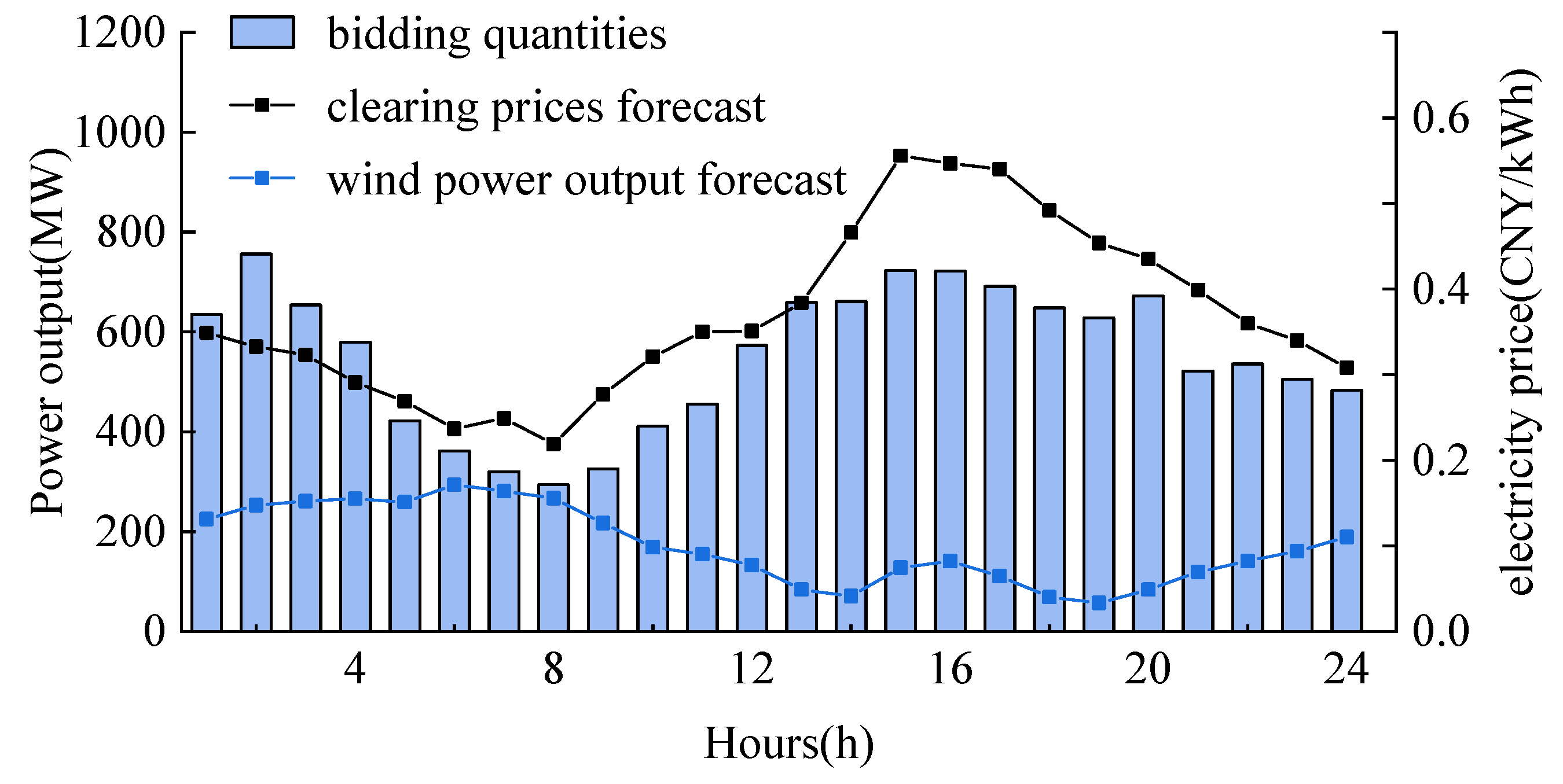
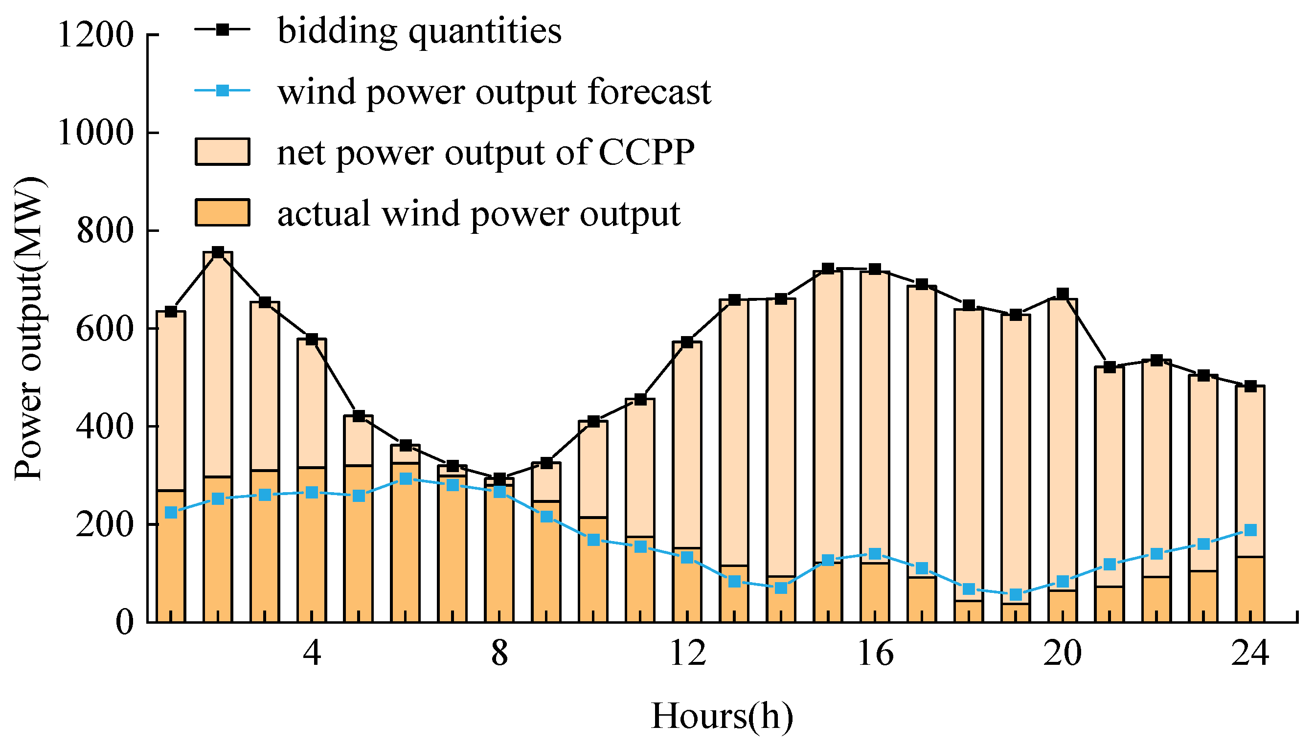
The case study uses a 600 MW CCPP and a 370 MW wind farm. The detailed parameters for the thermal power unit of the carbon capture plant are shown in Appendix A, Table A1, and the parameters for the carbon capture facilities are referenced from [22]. The generation cost coefficient of the wind farm is CNY 100/MWh. The penalty coefficients for positive and negative imbalances are 0.4 and 1.6, respectively. The carbon emission baseline per unit of electricity is 0.7 t/(MW·h), with a carbon trading benchmark price of CNY 100/t, a compensation coefficient of 0.1, and a penalty coefficient of 0.2. The interval length of carbon emission rights is 2000 t. The forecast results for wind power output and day-ahead clearing price are shown in Figure 3, with standard deviations of the forecast errors set at 25% and 15%, respectively. The Monte Carlo method is used for random sampling to generate 1000 wind power out and price scenarios. Employing scenario reduction techniques, the scenarios are reduced to 10 typical ones, each with its corresponding probability. The risk aversion coefficient δ = 1, and the CVaR confidence level β = 0.95. The model is solved using MATLAB software R2016b and the Gurobi optimizer 10.0.0.
4.1. Analysis of Bidding Results
Figure 3 illustrates the results of joint bidding under the risk-averse strategy. As depicted in Figure 3, from hours 5 to 9, wind power is abundant, and the predicted power output of the wind farm is substantial, yet the bidding quantities are relatively low. This is attributed to the lower electricity price during this period, which is close to the marginal cost of the thermal power unit, so the bidding quantities are relatively low. At the same time, in periods when the electricity price is high, the bidding quantities increase to maximize revenue from electricity sales. This enables the generation alliance to achieve profitability throughout the entire day. Additionally, limited by weather conditions such as wind speed, the inclusion of the thermal power unit also somewhat weakens the counter-peak characteristics of wind power, enabling the generation alliance to respond to clearing price signals and formulate an hourly generation plan. It is evident that the hourly bidding quantities align approximately with the trend of electricity price changes, thereby favoring a responsive approach to meet the market load demand.
Figure 3.
Optimized bidding results in the day-ahead market.

The bidding strategy takes into account revenues from both the day-ahead market and real-time balancing market settlements, providing a comprehensive decision-making perspective. The balancing market aims to eliminate imbalanced electricity. Given the strict penalties for generation shortage and wind curtailment, day-ahead bidding is conservative. Under an individual bidding strategy, the wind farm submits a generation plan based on the optimization results considering day-ahead revenues and real-time balancing market revenues for the scenario set. In the case of individual bidding by the CCPP, it assumes no power output deviation. Due to the higher costs associated with the thermal power unit compared to wind power, the CCPP facilitates the integration of wind power into the grid, thereby reducing overall operating costs. This results in joint bidding yielding higher profits than individual bidding, with lower risks associated with joint bidding compared to individual bidding.
According to Table 1, the total expected profits and total CVaR for individual bidding are CNY 1675.3 thousand and CNY 1547.6 thousand, respectively, while for joint bidding, they are CNY 1790.9 thousand and CNY 1647.9 thousand, with gains of CNY 115.6 thousand and CNY 100.3 thousand, respectively. Given the prioritization of wind power for grid integration under this strategy, thermal power inevitably stands to lose the profits it would have gained under individual bidding during the coordination process. Without adequate compensation, participating in joint bidding would be contrary to the interests of thermal power stakeholders. Using the Shapley value [23] to fairly allocate the total profits, Table 2 shows the profit for each member. The expected profit for wind power is CNY 875.3 thousand, an increase of 7.07%, while for thermal power, it is CNY 915.6 thousand, an increase of 6.74%. The analysis above demonstrates that the adoption of Shapley’s value ensures mutually beneficial outcomes for participating members.
4.2. Comparison of Different Cases
This section considers the deployment of power generation alliance options. Three cases are considered: case 1 adopts the integrated flexible CCPP, equipped with solvent storage tanks. Case 2 employs a traditional CCPP, lacking solvent storage tanks. Case 3 refers to a conventional thermal power plant without carbon capture facilities.
Comparing the bidding results of each case with an individual wind farm, as shown in Table 2, it is evident that case 1 achieved the best results in both economic and low-carbon. The expected profit for case 1 increased by CNY 62.2 thousand and CNY 140.7 thousand compared to cases 2 and 3, respectively. Additionally, carbon trading costs decreased by CNY 622.5 thousand and CNY 1050.3 thousand, respectively, confirming that CCPPs have significantly lower carbon emission intensity compared to conventional thermal power plants.
Due to the fact that both case 1 and case 2 supply energy for the carbon capture system, the fuel costs are higher than those of case 3. However, the differences between the revenues from day-ahead market bidding and the total costs for case 1 and case 2 are, respectively, CNY 1810.8 thousand and CNY 1765.2 thousand, while for case 3, it is only CNY 1715.6 thousand. Thus, the economic feasibility of carbon capture power plants is ensured.
The carbon trading costs under conditions without and with solvent storage tanks are CNY 96.7 thousand and CNY −525.8 thousand, respectively, and the solvent loss costs are CNY 57.0 thousand and CNY 128.1 thousand, respectively. This implies that solvent storage tanks have increased the amount of CO2 that can be captured. The amount of net carbon emissions for case 1 is lower than the amount of corresponding carbon allowances, allowing the CCPP to benefit in the carbon trading market and thus bringing additional revenue. Furthermore, case 3 submitted the least total bidding amount in the day-ahead market compared to case 2. The reason is that the conventional thermal power plant has a high carbon emission intensity, and to avoid incurring high carbon trading costs from the tiered carbon trading mechanism, they reduced the electricity generation amount. Case 1′s total bidding amount is less than case 2, allowing it to provide greater adjustment capacity during the real-time stage.
The individual wind farm’s positive and negative imbalances settlement in the balancing market were CNY 51.8 thousand and CNY −182.3 thousand, respectively, while for case 3, they were CNY 16.7 thousand and CNY −82.2 thousand, respectively. This indicates that the joint bidding mode can mitigate wind power output deviations. The imbalance settlements for the three cases decreased in sequence, with case 1′s imbalance settlements being CNY 1.8 thousand and CNY −21.7 thousand, respectively. This demonstrates that case 1 has the smallest imbalance of electricity amount, thus promoting wind power grid integration to a greater extent. It also further illustrates that CCPPs consider solvent storage tanks to offer a more flexible operation, with a stronger capability to facilitate the integration of wind power compared to conventional thermal power plants and traditional CCPPs.

Table 2.
Comparison of different cases.
| Unit | Case 1 | Case 2 | Case 3 | Individual Wind Farm | |
|---|---|---|---|---|---|
| Total Bidding Amount | MWh | 13238 | 14947 | 14105 | 4012 |
| Day-Ahead Market Revenue | Thousand (CNY) | 5123.0 | 5663.4 | 5477.2 | 1358.4 |
| Fuel Cost | Thousand (CNY) | 3299.6 | 3334.3 | 2726.7 | — |
| Solvent Loss Cost | Thousand (CNY) | 128.1 | 57.0 | — | — |
| Start-up and Shutdown Costs for Thermal Power Units | Thousand (CNY) | 0 | 0 | 100.0 | — |
| Carbon Trading Cost | Thousand (CNY) | −525.8 | 96.7 | 524.5 | — |
| Total Cost | Thousand (CNY) | 3312.2 | 3898.2 | 3761.6 | 410.3 |
| Positive Imbalance Settlement | Thousand (CNY) | 1.8 | 3.3 | 16.7 | 51.8 |
| Negative Imbalance Settlement | Thousand (CNY) | −21.7 | −39.7 | −82.2 | −182.3 |
| Expected Profit | Thousand (CNY) | 1790.9 | 1728.7 | 1650.2 | 817.5 |
4.3. Analysis of Risk Preference
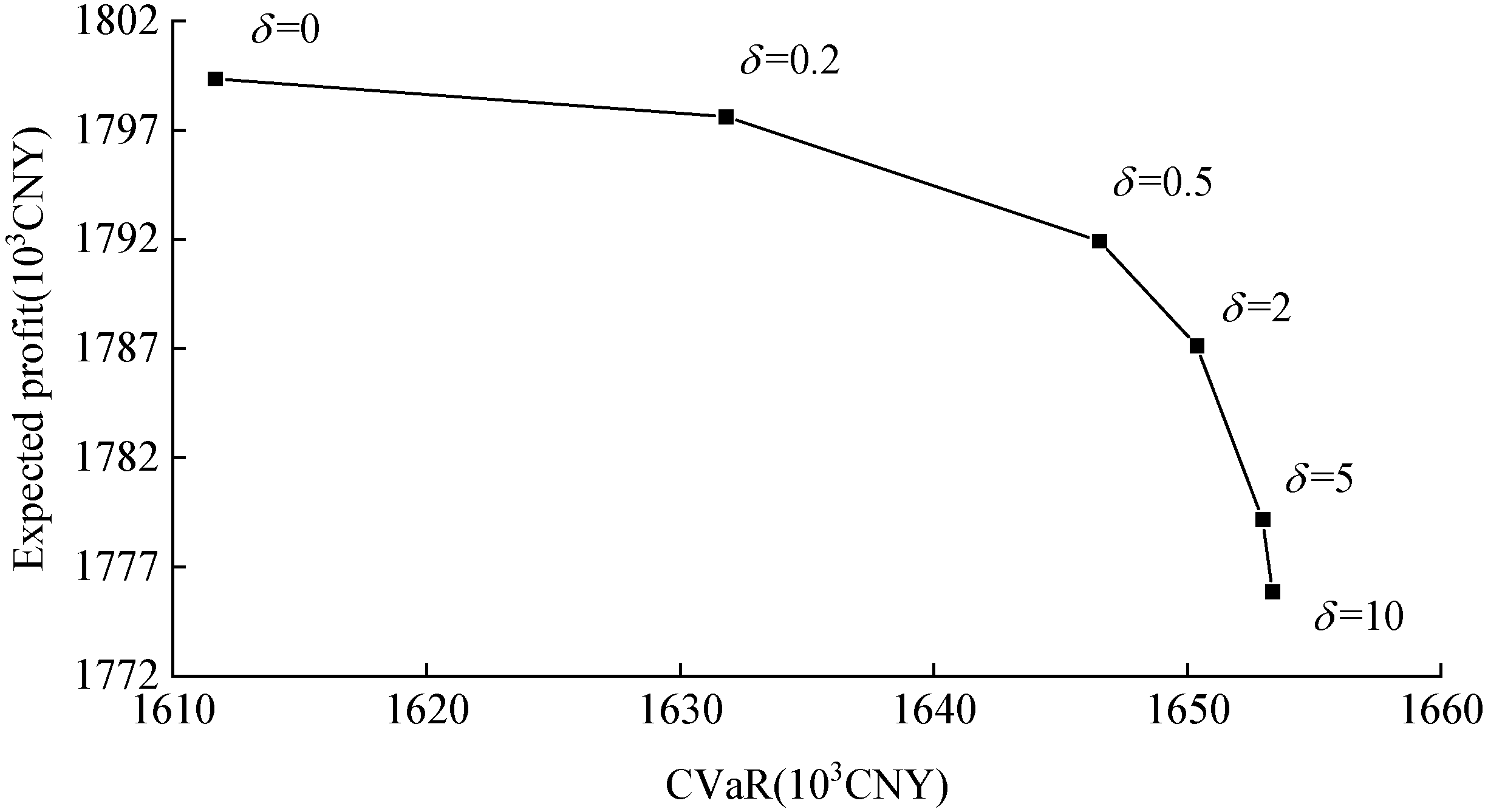
This section explores the expected profits and CVaR values under different risk aversion coefficients, with δ values ranging from 0 to 10. Figure 4 illustrates the efficient frontier curve of CVaR, where a δ value of 0 represents a risk-neutral attitude, focusing solely on maximizing bidding profits. It is observed that the joint bidding strategy, when not considering risk, achieves a maximum expected profit of CNY 1799.4 thousand, which is CNY 23.5 thousand higher than the strong risk-averse joint bidding strategy (δ is 10). The purpose of risk aversion is to reduce the expected profit gap between different scenarios by sacrificing economic benefits. Hence, the resulting CVaR value when δ is 10 is CNY 1653.3 thousand, which is an increase of CNY 41.7 thousand compared to the situation when δ is 0.
As the δ value increases, the expected profit exhibits a declining trend, while CVaR shows an ascending trend. This implies a positive correlation between risk and profit, wherein decision-makers aiming for higher profits also face greater risks. Within the δ range of 1 to 10, the decision-making objective shifts from balancing profits and risks (δ = 1) to placing a stronger emphasis on risk (δ > 1). As δ increases, the CVaR value grows, accompanied by a significant decrease in expected profits. The bidding strategy becomes more focused on the tail of the profit distribution under a given confidence level. Therefore, it is necessary to measure the risk attitude of decision-makers in bidding and find the optimal balance between risk and revenue, thereby formulating appropriate bidding strategies for market participants.
4.4. Analysis of the Flexible Operation Characteristics of CCPP
The power generation alliance needs to strategically determine its power output based on the bidding quantities and day-ahead clearing price. Figure 5 illustrates the actual power output of the wind farm and CCPP. Between hours 1 to 6, in cases where wind power output exceeds its forecast, the CCPP minimizes wind power curtailment by reducing its net power output. The carbon capture system can serve as a dispatchable load. From hours 5 to 10, the net power output of the thermal power unit is significantly below its minimum technical output. Between hours 18 and 24, the CCPP compensates for the shortage in wind power output, aiming to closely align the actual power generation quantities of the generation alliance with the day-ahead bidding quantities (day-ahead generation plan).
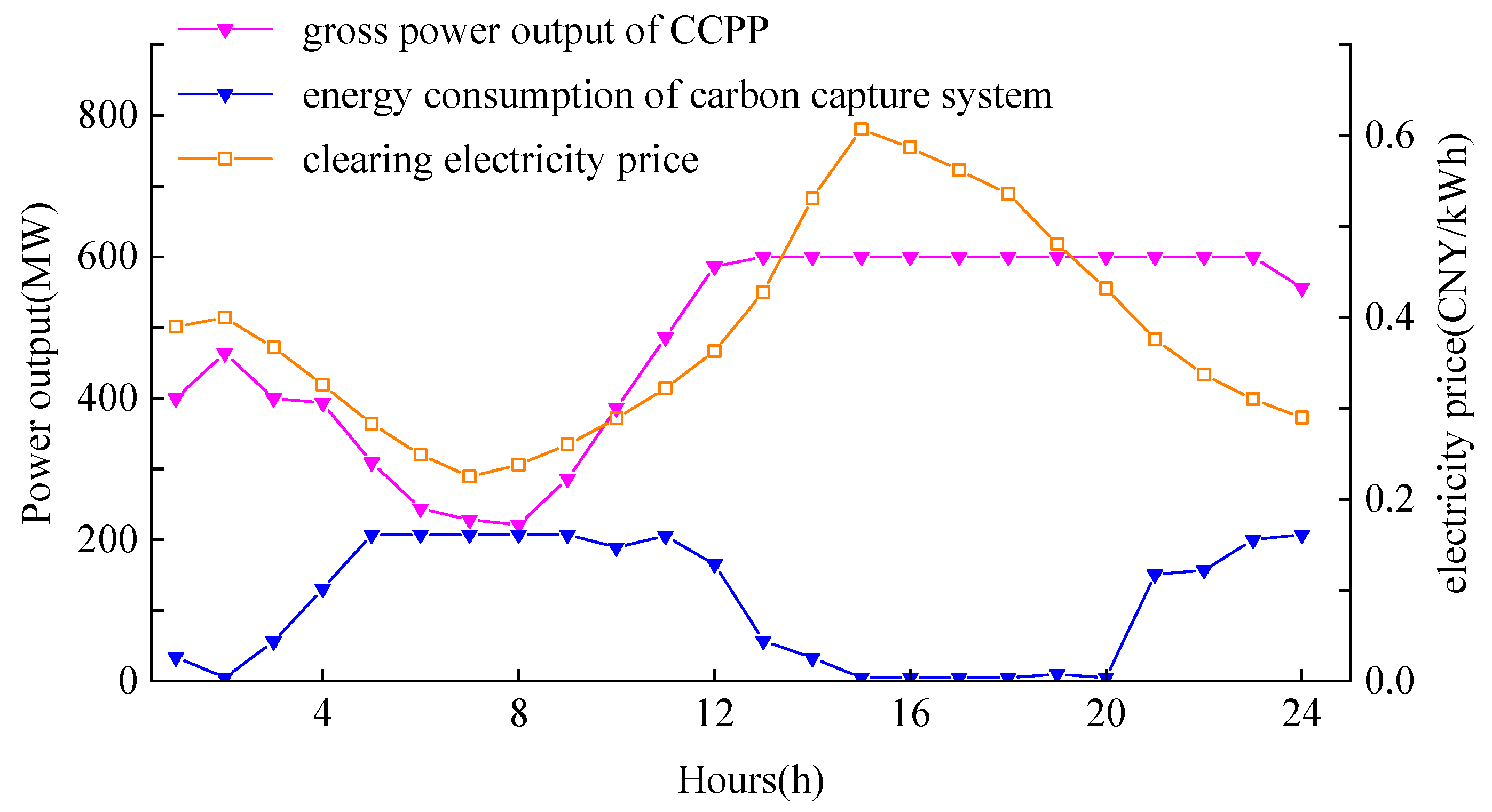
To further investigate the flexible operation mechanism of CCPP, an analysis of the power output and carbon flow is conducted. As shown in Figure 6, the net power output of a CCPP is the difference between its gross power output and the energy consumption of the carbon capture system. During low electricity price periods, it is observed that CCPP tend to increase the energy supply to carbon capture systems. This strategy is motivated by the opportunity to capture CO2 and obtain revenue by selling the excess carbon allowances in the carbon trading market.
Conversely, during periods of high prices, the CCPP increases its net power output by raising its gross output and reducing the energy supply to the capture system. This strategy is motivated by the significantly higher revenue in the electricity spot market during these times, making it economically advantageous to sell electricity. In summary, the analysis reveals that the generation preferences of the CCPP depend on electricity prices. By adjusting the energy supply to the carbon capture system, the CCPP can flexibly modify net power output, enabling it to operate at an economically optimal point. The adoption of distinct strategies during peak and off-peak electricity prices is crucial for maximizing profits throughout the entire operational cycle.
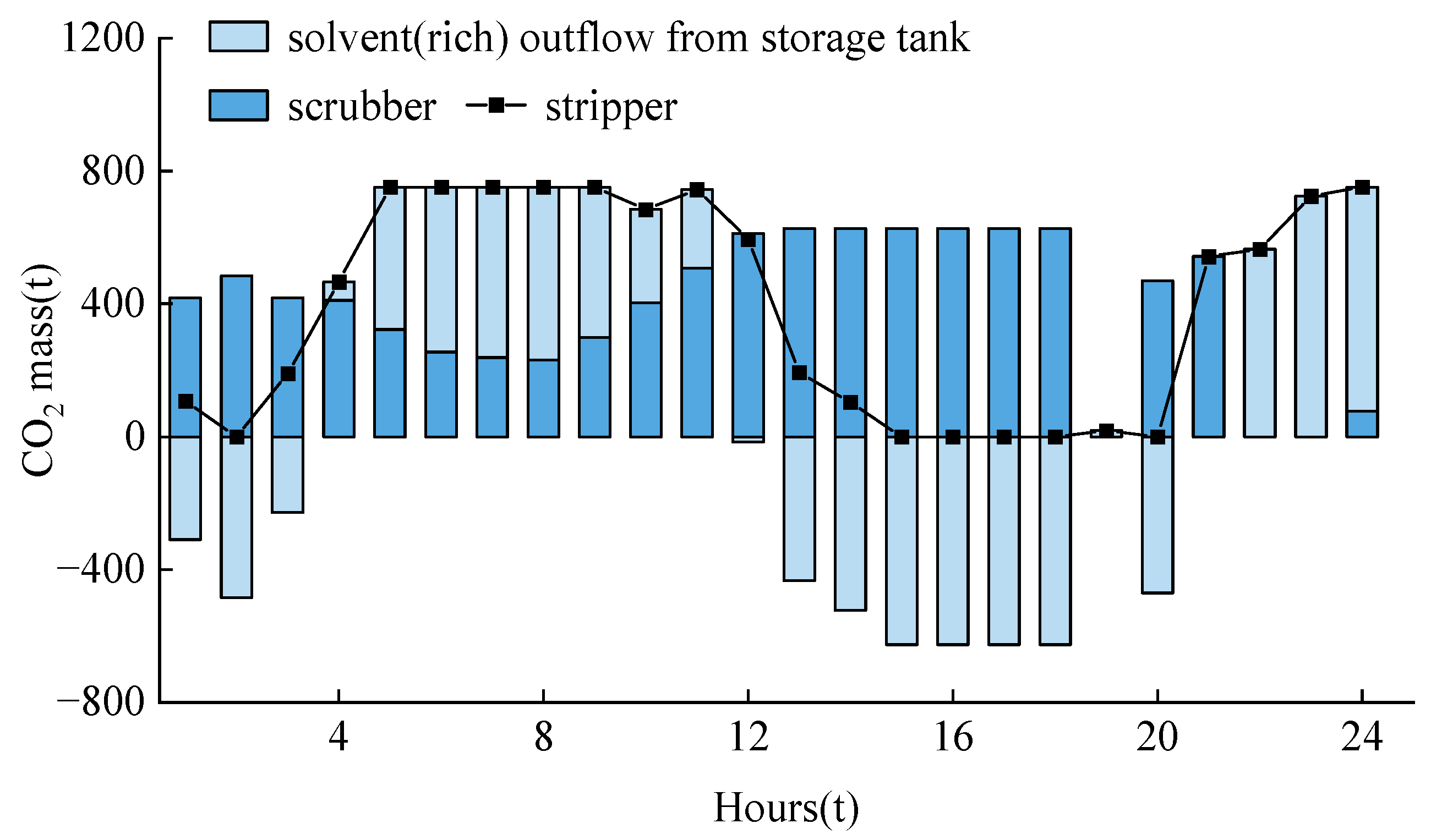
As indicated by Figure 7, the scrubber and stripper of the integrated flexible CCPP no longer operate synchronously due to the installation of the solvent storage tank. During low electricity price periods, as the output of the thermal power unit decreases, the amount of CO2 produced by the plant also decreases. Consequently, a carbon capture system, functioning as a dispatchable load to absorb excess electricity, may not have a sufficient supply of CO2 for capture during such periods. From hours 4 to 11, as depicted in Figure 7, there is a reduction in the volume of the “rich” solvent in the tank, as solvents from the scrubber and “rich” solvent tank are transferred to the stripper. This leads to a substantial increase in carbon capture energy consumption, leading to a significant reduction in the net power output of the CCPP.
During peak electricity price periods, the CCPP requires a higher net power output to meet the day-ahead generation plan. Simultaneously, the plant will also produce a significant amount of CO2. The CCPP increases the flue gas entering the scrubber and stores the absorbed CO2 inside the “rich” solvent tank. This not only reduces emissions of CO2 into the atmosphere but also reduces the energy supply to the carbon capture system by storing CO2 without immediate capture. As a consequence, during these periods, the volume of solvent processed within the stripper decreases, resulting in an increase in the net power output of the CCPP. Finally, the volumes of both the lean and rich solvents in the storage tank are restored to their initial levels at the end of the cycle, ensuring the long-term operation of the carbon capture system.
4.5. Comparison of Results between MILP and MINLP
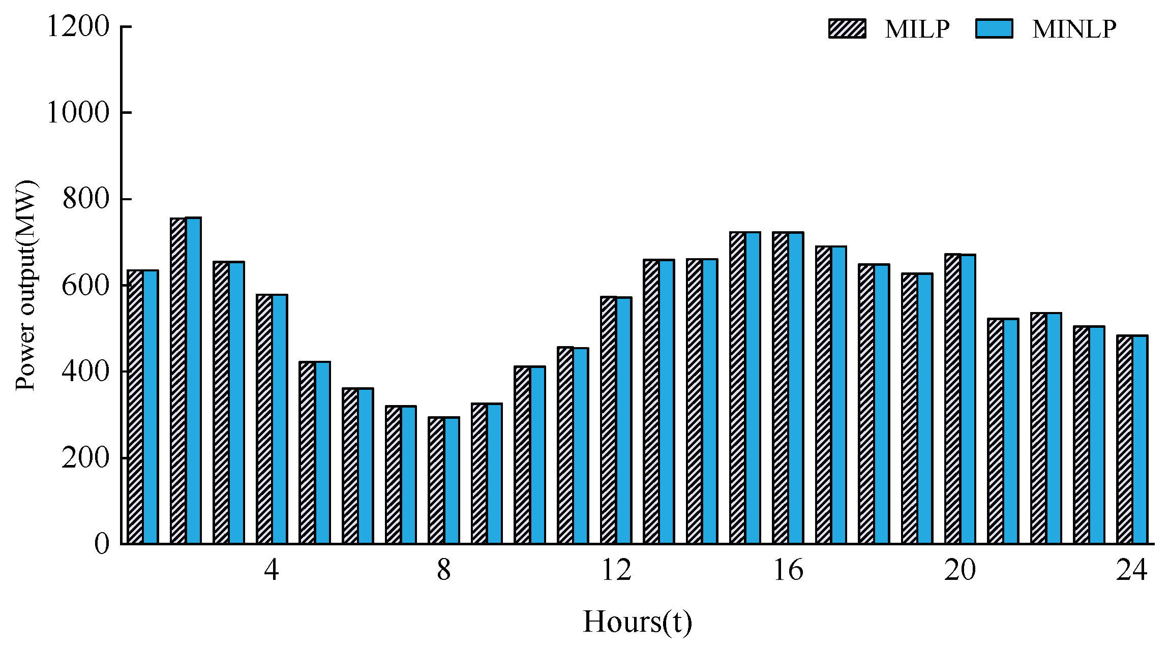
Table 3 compares the solution results of the MILP and MINLP models using the Gruobi optimizer. As shown in Table 3, compared to the MILP model, which was solved in 15.61 s, the MINLP solution was obtained in 1443.37 s. Regarding results accuracy, the MILP optimization results in an objective function value of 3438.9, while MINLP optimization yields a value of 3440.8, with a mere difference of 1.9 between the two. The difference between the two objective function values is rather small. As depicted in Figure 8, the optimal bidding electricity quantities in the day-ahead market obtained from MILP and MINLP are rather similar. In summary, based on the comparison of the exact optimal solution between the MILP and MINLP approaches, MILP can find acceptable exact solutions in our bidding problem much faster, demonstrating that the MILP approach holds advantages over the MINLP technique from the viewpoint of solution time.
5. Conclusions
Currently, China is in the early stages of constructing electricity spot markets and carbon trading markets. In anticipation of wind power participating in the electricity spot market in the future, a two-stage decision-making model is established, which combines CCPP and wind farm bidding in the spot market to mitigate the imbalance costs under the uncertainty of wind power output. The specific conclusions are as follows:
- (1)
- Compared to individual bidding, the joint wind-thermal bidding strategy reduces risk while obtaining excess profits in the spot market.
- (2)
- This paper compares three cases and verifies that the integrated flexible CCPP has clear advantages in terms of economy, low carbon emissions, and wind power integration. This is attributed to the installation of a solvent tank, which not only enhances the flexibility of the CCPP but also improves energy utilization efficiency. Thus, it deeply reduces carbon emissions while optimizing economic benefits.
- (3)
- The decision model facilitates risk control, providing a comparative result for decision-makers to choose different risk coefficients. A risk-averse model has been established, demonstrating a proportional relationship between risk and profit. This can provide a better reference for market bidding.
- (4)
- This study considers wind farms and CCPPs as price takers jointly participating in the spot market. As regional market trading rules continue to evolve and develop, and with the increasing share of renewable energy participation in the market, future work will focus on the price-making strategies of power generators.
Author Contributions
Conceptualization, Z.L.; Methodology, Z.L.; Software, Z.L.; Validation, Z.L.; Writing—original draft, W.T.; Writing—review and editing, B.W.; Supervision, Y.L. All authors have read and agreed to the published version of the manuscript.
Funding
This research was funded by the National Key Research and Development Program of China (2022YFB2403503).
Data Availability Statement
The data presented in this study are available on request from the corresponding author due to privacy.
Acknowledgments
Zhiwei Liao thanks Wenjuan Tao, Bowen Wang, and Ye Liu for their valuable discussions and their helpful advice with this paper.
Conflicts of Interest
The authors declare no conflicts of interest.
Appendix A
Table A1.
Parameters of thermal power units.
| Parameter | Unit | Value | Parameter | Unit | Value |
|---|---|---|---|---|---|
| Coal Cost Coefficient a | CNY/MW2·h | 0.012 | Carbon Emission Intensity | t/MW∙h | 1.16 |
| Coal Cost Coefficient b | CNY/MW·h | 250 | Ramp Rate | MW/h | 100 |
| Coal Cost Coefficient c | CNY | 8700 | Per Start-up and Shutdown Cost | Thousand CNY | 50 |
| Maximum Technical Output | MW | 600 | Minimum Start-up and Shutdown Time | h | 4 |
| Minimum Technical Output | MW | 200 |
References
- Li, Z.; Chen, S.Y.; Dong, W.; Liu, P.; Du, E.; Ma, L.; He, J. Low Carbon Transition Pathway of Power Sector under Carbon Emission Constraints. Proc. CSEE 2021, 41, 3987–4000. [Google Scholar]
- National Development and Reform Commission, National Energy Administration. Notice on Actively Promoting the Work of Wind Power and Photovoltaic Power Generation Grid Interconnection without Subsidies at Parity [EB/OL]. Available online: https://www.nea.gov.cn/2019-01/10/c_137731320.htm (accessed on 17 January 2024).
- Ahmed, S.D.; Al-Ismail, F.S.M.; Shafiullah; Al-Sulaiman, F.A.; El-Amin, I.M. Grid integration challenges of wind energy: A review. IEEE Access 2020, 8, 10857–10878. [Google Scholar] [CrossRef]
- Wu, Z.; Zhou, M.; Li, G.; Zhao, T.; Zhang, Y.; Liu, X. Interaction between balancing market design and market behaviour of wind power producers in China. Renew. Sustain. Energy Rev. 2020, 132, 110060. [Google Scholar] [CrossRef]
- Xu, X.; Wang, H.; Yan, Z.; Lu, Z.; Kang, C.; Xie, K. Overview of Power System Uncertainty and Its Solutions under Energy Transition. Autom. Electr. Power Syst. 2021, 45, 2–13. [Google Scholar]
- Dadashi, M.; Zare, K.; Seyedi, H.; Shafie-Khah, M. Coordination of wind power producers with an energy storage system for the optimal participation in wholesale electricity markets. Int. J. Electr. Power Energy Syst. 2022, 136, 107672. [Google Scholar] [CrossRef]
- Cao, D.; Hu, W.; Xu, X.; Dragičević, T.; Huang, Q.; Liu, Z.; Chen, Z.; Blaabjerg, F. Bidding strategy for trading wind energy and purchasing reserve of wind power producer–A DRL based approach. Int. J. Electr. Power Energy Syst. 2020, 117, 105648. [Google Scholar] [CrossRef]
- Alashery, M.K.; Xiao, D.; Qiao, W. Second-order stochastic dominance constraints for risk management of a wind power producer’s optimal bidding strategy. IEEE Trans. Sustain. Energy 2019, 11, 1404–1413. [Google Scholar] [CrossRef]
- Yang, B.; Tang, W.; Wu, F.; Wang, H.; Sun, W. Day-ahead market bidding strategy for “renewable energy + energy storage” power plantsconsidering conditional value-at-risk. Power Syst. Prot. Control. 2022, 50, 93–101. [Google Scholar]
- Wang, H.; Chen, J.; Zhu, T.; Wu, M.; Chen, Q.; Zhu, J.; Liu, M. Joint Bidding Model and Algorithm of Wind-storage System Considering Energy Storage Life and Frequency Regulation Performance. Power Syst. Technol. 2021, 45, 208–215. [Google Scholar]
- Zhang, Q.; Wu, X.; Deng, X.; Huang, Y.; Li, C.; Wu, J. Bidding strategy for wind power and Large-scale electric vehicles participating in Day-ahead energy and frequency regulation market. Appl. Energy 2023, 341, 121063. [Google Scholar] [CrossRef]
- He, S.; Wang, L.; Zhao, S. Stochastic Cournot Game Based Distributed Optimization Strategy for Joint Bidding of Demand Response Aggregator and Multi-stakeholder Wind Power Producers. Power Syst. Technol. 2022, 46, 4789–4799. [Google Scholar]
- Wu, Z.; Zhou, M.; Yao, S.; Li, G.; Zhang, Y.; Liu, X. Optimization Operation Strategy of Wind-storage Coalition in Spot Market Based on Cooperative Game Theory. Power Syst. Technol. 2019, 43, 2815–2824. [Google Scholar]
- Khaloie, H.; Abdollahi, A.; Shafie-Khah, M.; Siano, P.; Nojavan, S.; Anvari-Moghaddam, A.; Catalão, J.P. Co-optimized bidding strategy of an integrated wind-thermal-photovoltaic system in deregulated electricity market under uncertainties. J. Clean. Prod. 2020, 242, 118434. [Google Scholar] [CrossRef]
- Khaloie, H.; Abdollahi, A.; Shafie-Khah, M.; Anvari-Moghaddam, A.; Nojavan, S.; Siano, P.; Catalão, J.F.S. Coordinated wind-thermal-energy storage offering strategy in energy and spinning reserve markets using a multi-stage model. Appl. Energy 2020, 259, 114168. [Google Scholar] [CrossRef]
- Peng, F.; Sui, X.; Hu, S.; Zhou, W.; Sun, H.; Chen, X. Joint bidding Strategy for Wind and Thermal Power Based on Information Gap Decision Theory. Power Syst. Technol. 2021, 45, 3379–3388. [Google Scholar]
- Xi, H.; Zhu, M.; Lee, K.Y.; Wu, X. Multi-timescale and control-perceptive scheduling approach for flexible operation of power plant-carbon capture system. Fuel 2023, 331, 125695. [Google Scholar] [CrossRef]
- Zhu, M.; Liu, Y.; Wu, X.; Shen, J. Dynamic modeling and comprehensive analysis of direct air-cooling coal-fired power plant integrated with carbon capture for reliable, economic and flexible operation. Energy 2023, 263, 125490. [Google Scholar] [CrossRef]
- Kou, Y.; Wu, J.; Zhang, H.; Yang, J.; Jiang, H. Low carbon economic dispatch for a power system considering carbon capture and CVaR. Power Syst. Prot. Control. 2023, 51, 131–140. [Google Scholar]
- Wang, X.; Gao, C. Two-stage Decision-making Model of Power Generation and Coal Purchase Arrangement for Power Generation Companies in Medium and Long-term Market. Power Syst. Technol. 2021, 45, 3992–3999. [Google Scholar]
- Khajavirad, A. On the strength of recursive McCormick relaxations for binary polynomial optimization. Oper. Res. Lett. 2023, 51, 146–152. [Google Scholar] [CrossRef]
- Cui, Y.; Deng, G.; Zhao, Y.; Zhong, W.; Tang, Y.; Liu, X. Economic Dispatch of Power System with Wind Power Considering the Complementarity of Low-carbon Characteristics of Source Side and Load Side. Proc. CSEE 2021, 41, 4799–4815. [Google Scholar]
- Wang, X.; Zhang, H.; Zhang, S.; Wu, L. Impacts of joint operation of wind power with electric vehicles and demand response in electricity market. Electr. Power Syst. Res. 2021, 201, 107513. [Google Scholar] [CrossRef]
Figure 1.
Carbon flow and energy flow of CCPP under the integrated, flexible operation mode.

Figure 2.
The decision-making framework.

Figure 4.
CVaR efficient frontier.

Figure 5.
Power output of the wind farm and CCPP.

Figure 6.
Power allocation of CCPP.

Figure 7.
Distribution of carbon flow in CCPPs.

Figure 8.
Comparison of the optimized bidding quantities in the day-ahead market.

Table 1.
Expected profit of individual bidding and joint bidding.
| Wind Power | Thermal Power | Total Expected Profits | Total CVaR | |
|---|---|---|---|---|
| Unit | Thousand (CNY) | Thousand (CNY) | Thousand (CNY) | Thousand (CNY) |
| Individual bidding | 817.5 | 857.8 | 1675.3 | 1547.6 |
| Joint bidding | 875.3 | 915.6 | 1790.9 | 1647.9 |
Table 3.
Comparison of solution results between MILP and MINLP.
| Solution Time/s | Objective Functions/ Thousand (CNY) | Expected Profit/ Thousand (CNY) | |
|---|---|---|---|
| MILP | 15.61 | 3438.9 | 1790.9 |
| MINLP | 1443.37 | 3440.8 | 1792.0 |
Disclaimer/Publisher’s Note: The statements, opinions and data contained in all publications are solely those of the individual author(s) and contributor(s) and not of MDPI and/or the editor(s). MDPI and/or the editor(s) disclaim responsibility for any injury to people or property resulting from any ideas, methods, instructions or products referred to in the content. |
© 2024 by the authors. Licensee MDPI, Basel, Switzerland. This article is an open access article distributed under the terms and conditions of the Creative Commons Attribution (CC BY) license (https://creativecommons.org/licenses/by/4.0/).
Share and Cite
MDPI and ACS Style
Liao, Z.; Tao, W.; Wang, B.; Liu, Y. Bidding Strategy for Wind and Thermal Power Joint Participation in the Electricity Spot Market Considering Uncertainty. Energies 2024, 17, 1714. https://0-doi-org.brum.beds.ac.uk/10.3390/en17071714
AMA Style
Liao Z, Tao W, Wang B, Liu Y. Bidding Strategy for Wind and Thermal Power Joint Participation in the Electricity Spot Market Considering Uncertainty. Energies. 2024; 17(7):1714. https://0-doi-org.brum.beds.ac.uk/10.3390/en17071714
Chicago/Turabian StyleLiao, Zhiwei, Wenjuan Tao, Bowen Wang, and Ye Liu. 2024. "Bidding Strategy for Wind and Thermal Power Joint Participation in the Electricity Spot Market Considering Uncertainty" Energies 17, no. 7: 1714. https://0-doi-org.brum.beds.ac.uk/10.3390/en17071714
Note that from the first issue of 2016, this journal uses article numbers instead of page numbers. See further details here.