A Comparative Study on Johnson Cook, Modified Zerilli–Armstrong, and Arrhenius-Type Constitutive Models to Predict Compression Flow Behavior of SnSbCu Alloy


Abstract
:1. Introduction
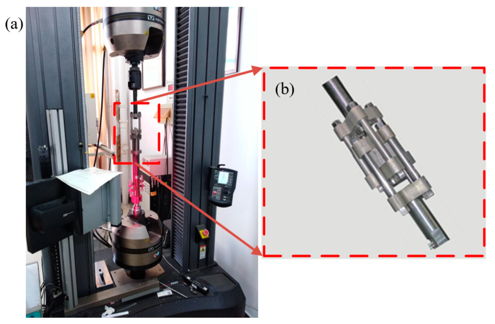
2. Experiment
3. Results and Discussions
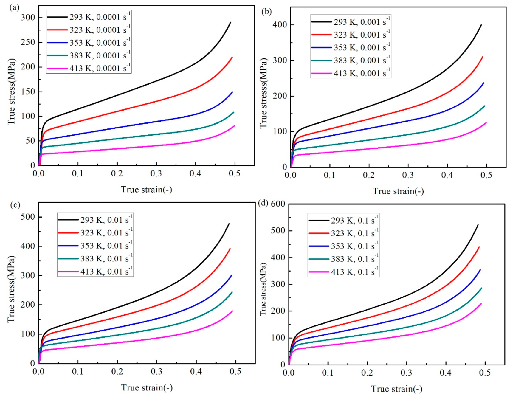
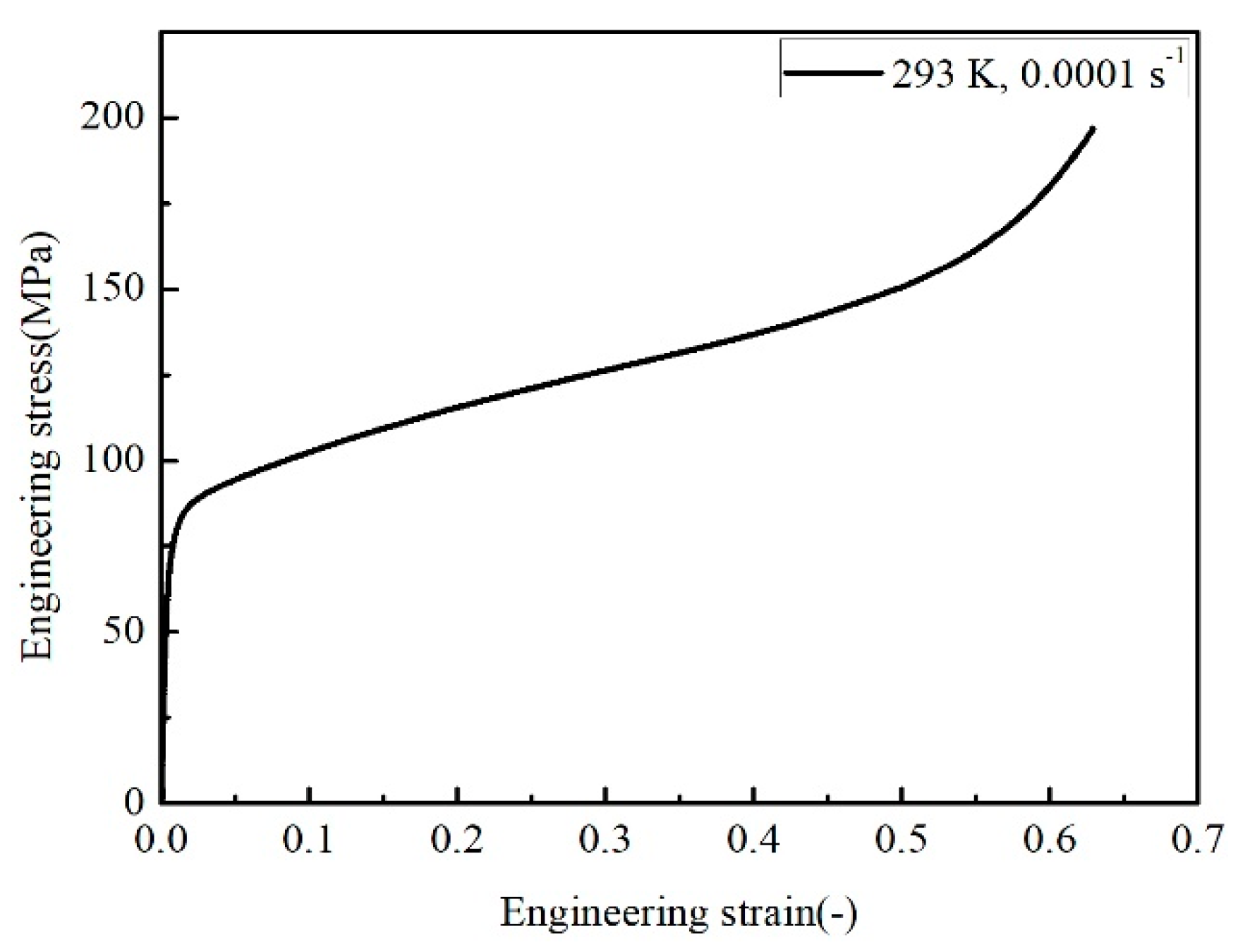
3.1. Experimental Results
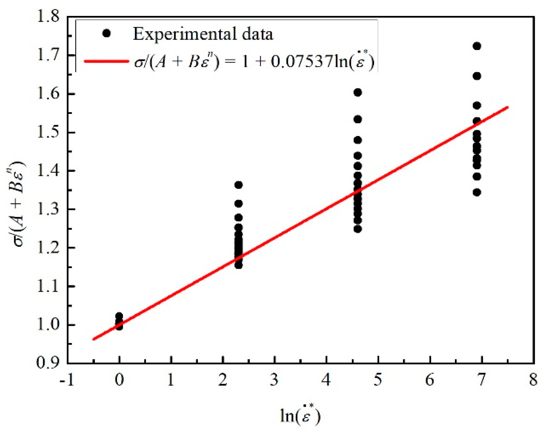
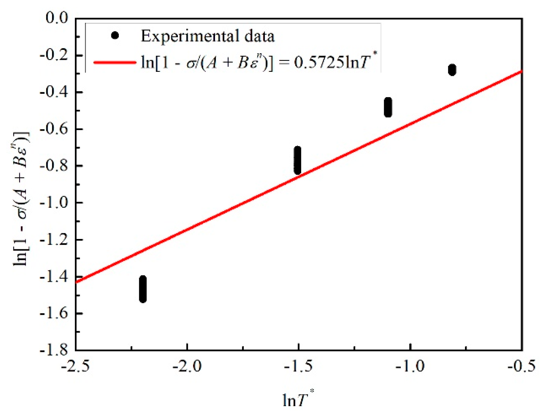
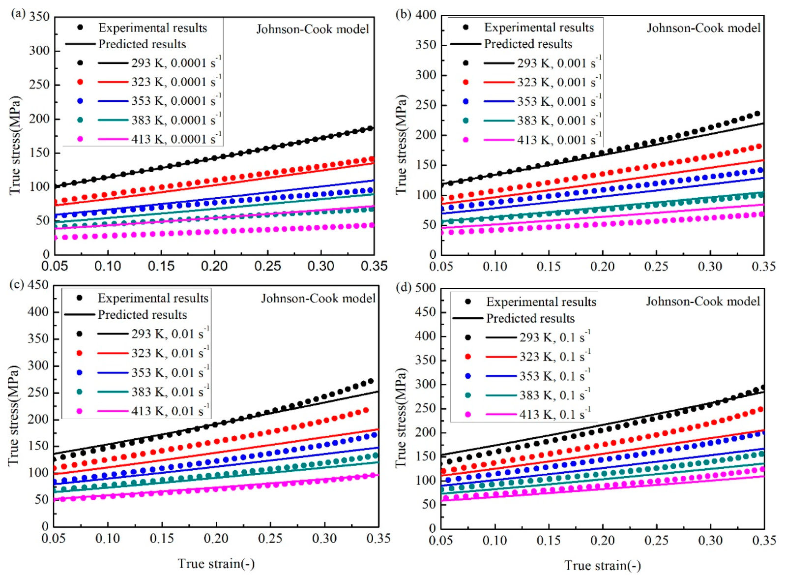
3.2. Johnson–Cook Model
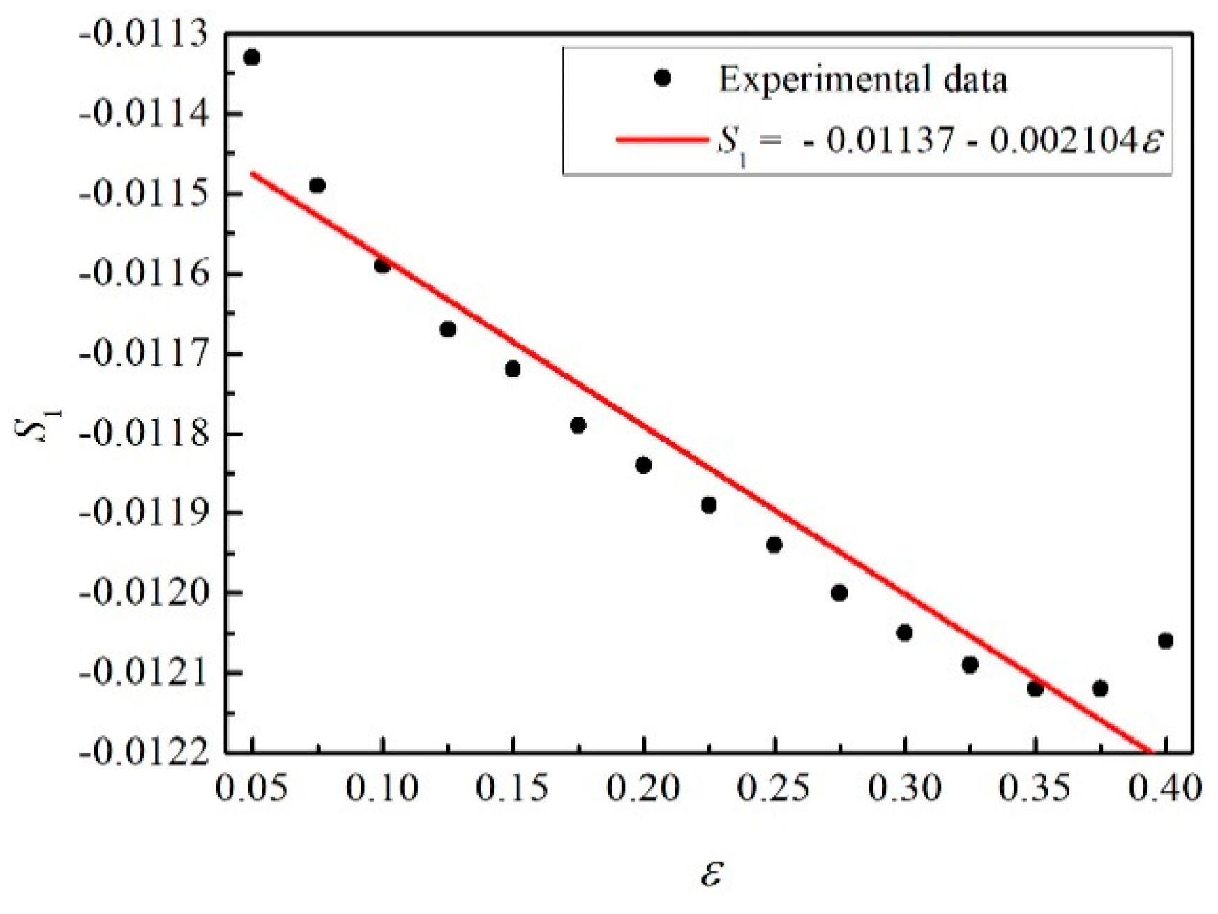
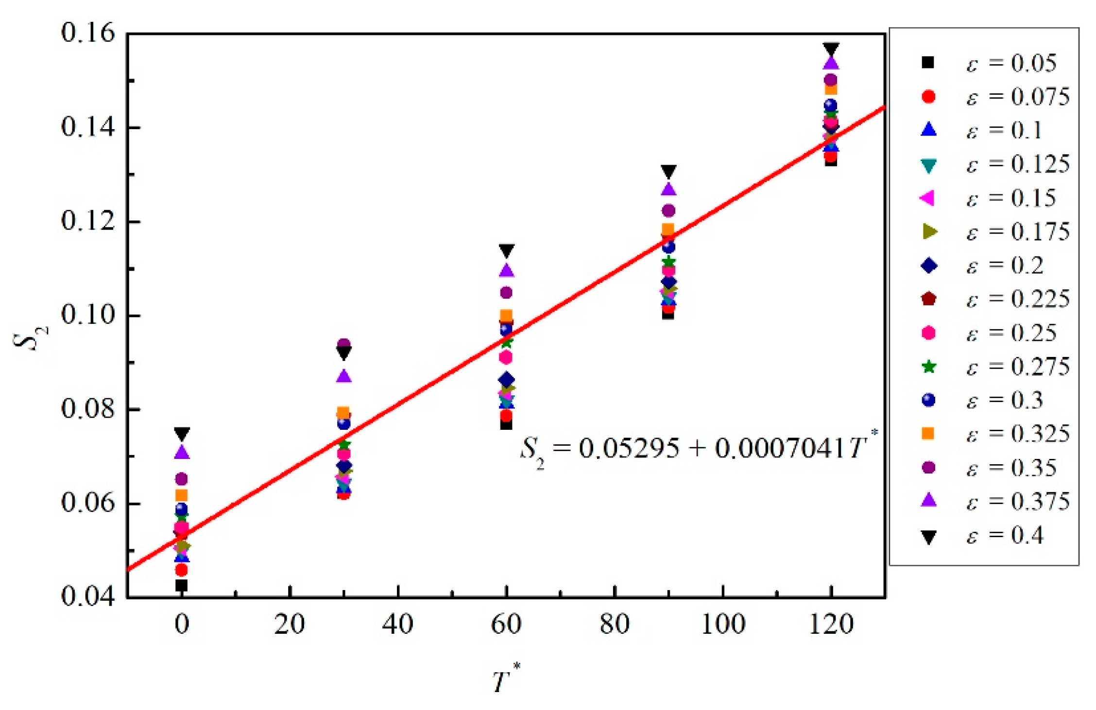
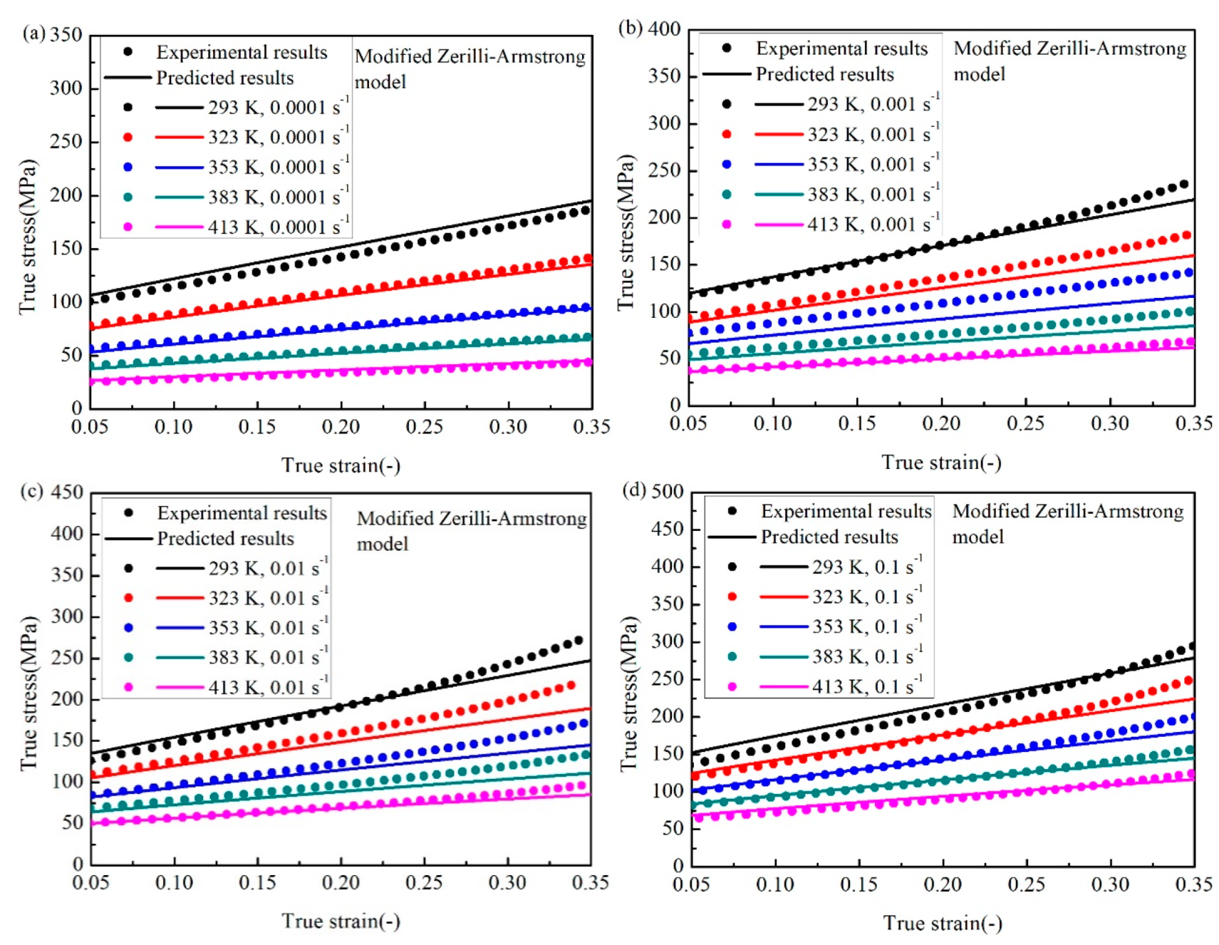
3.3. Modified Zerilli–Armstrong Model
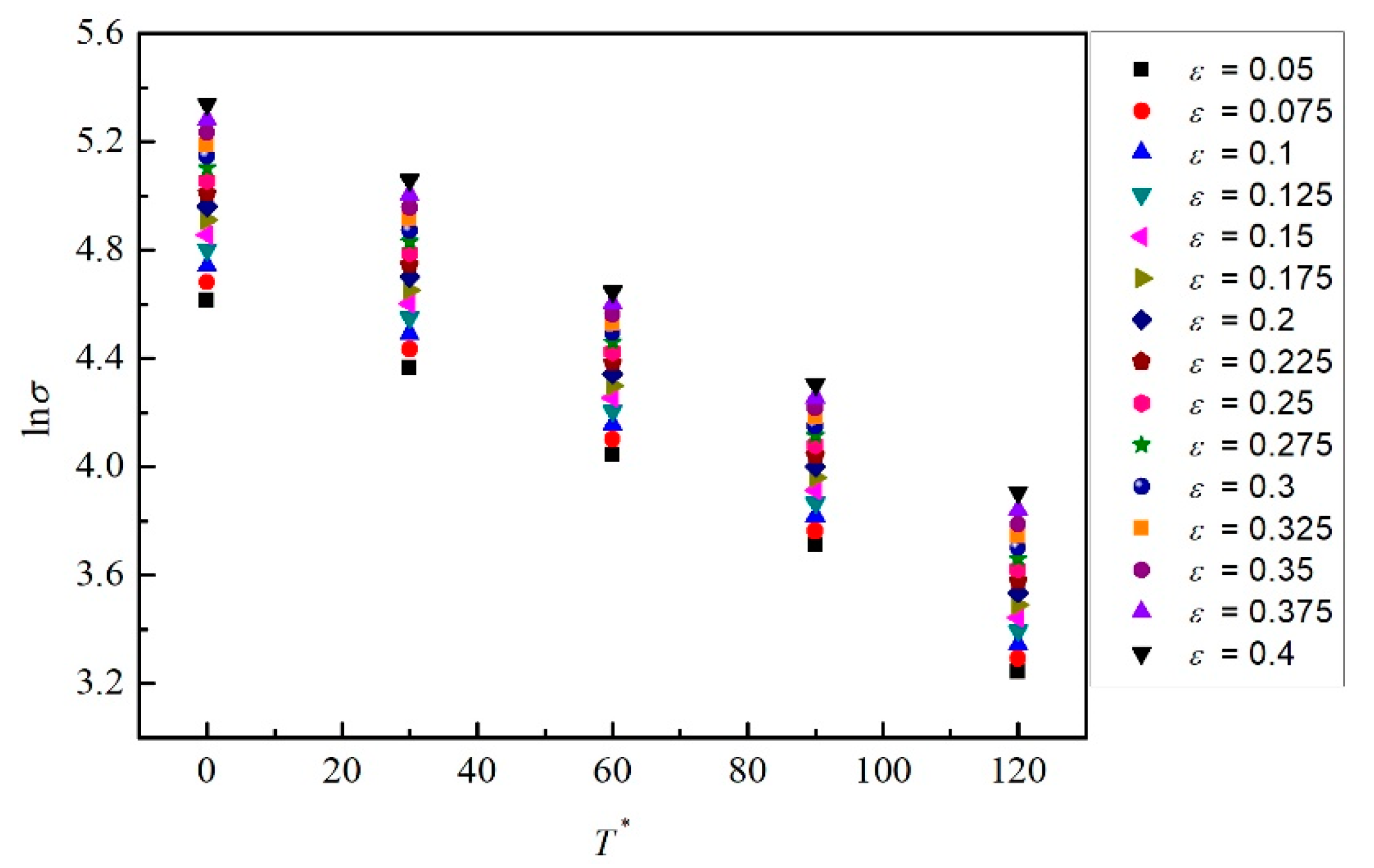
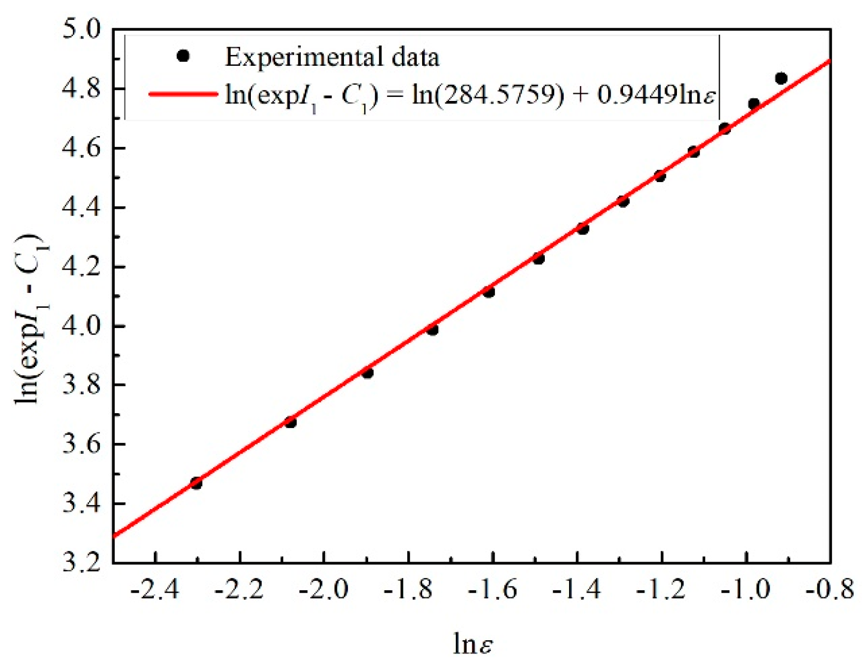
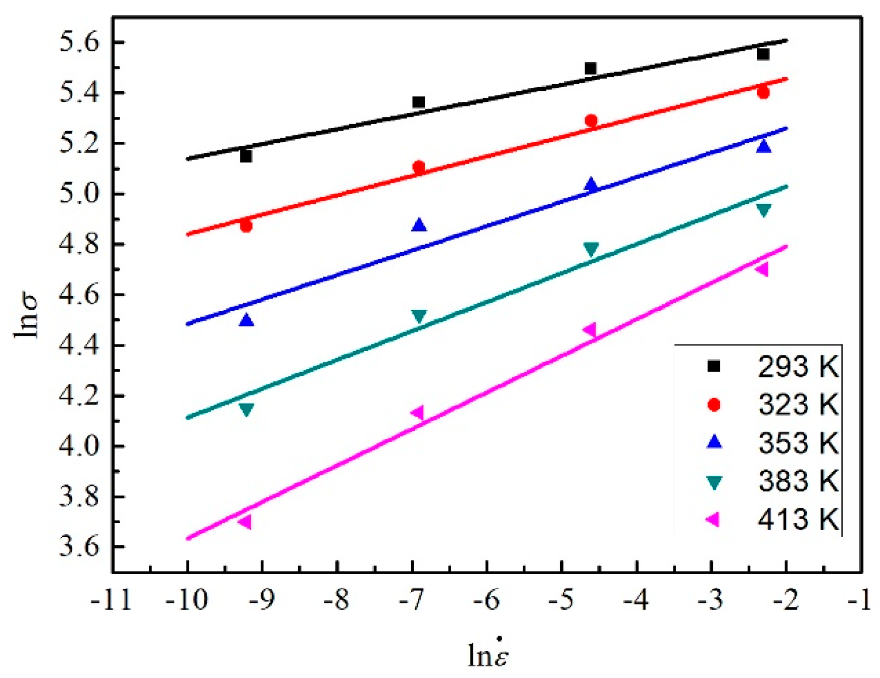
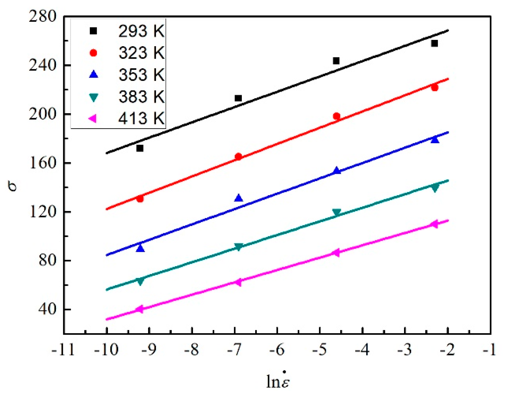
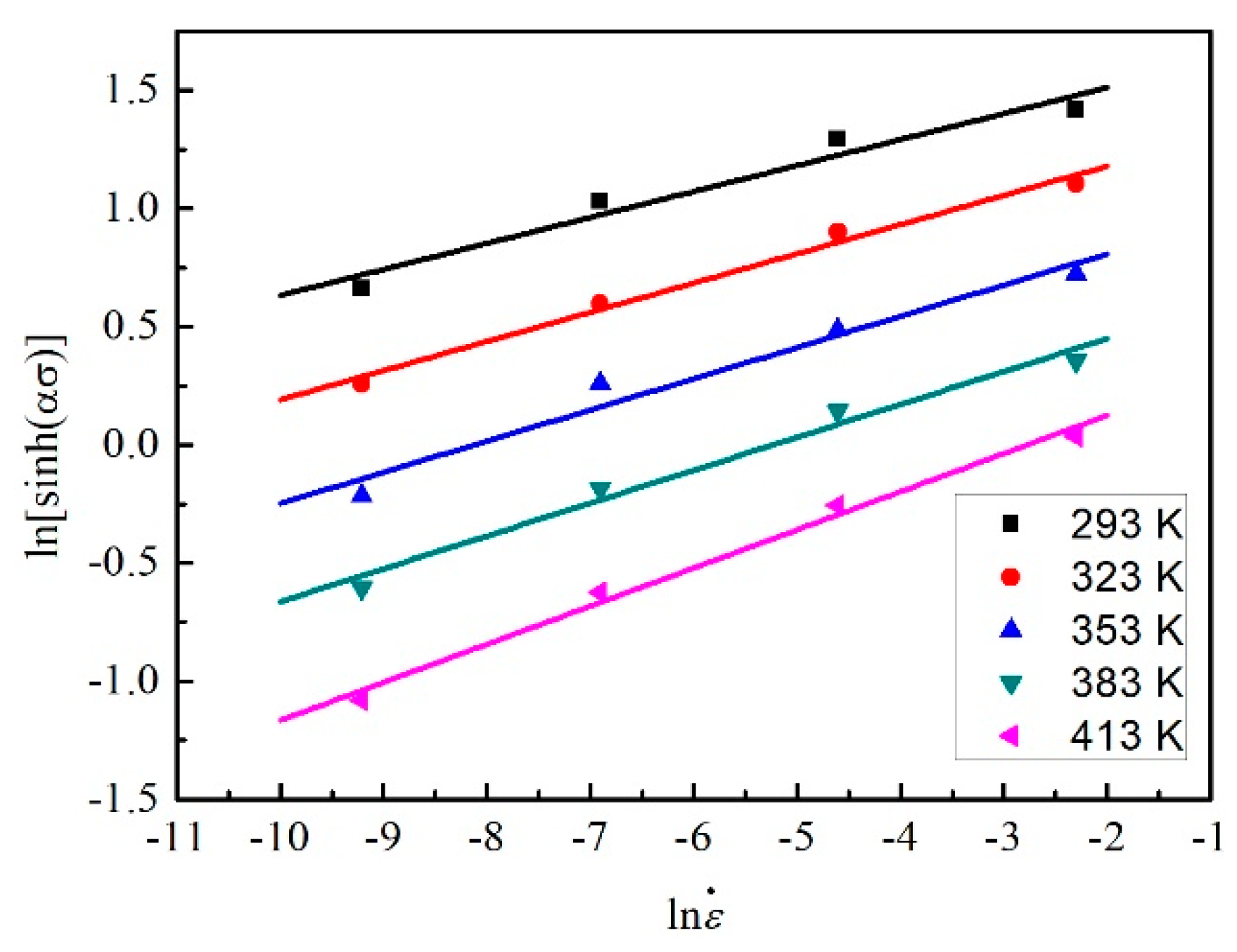
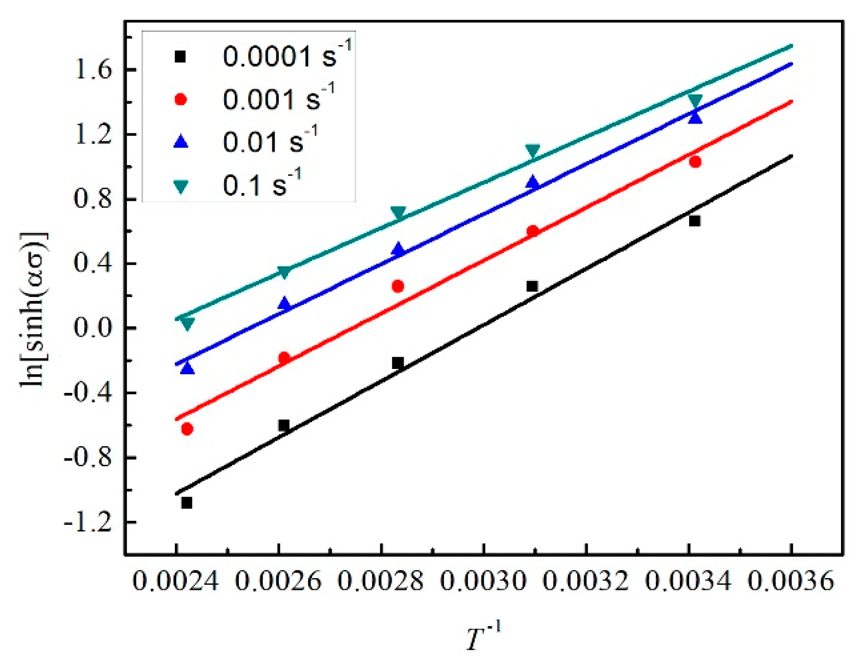
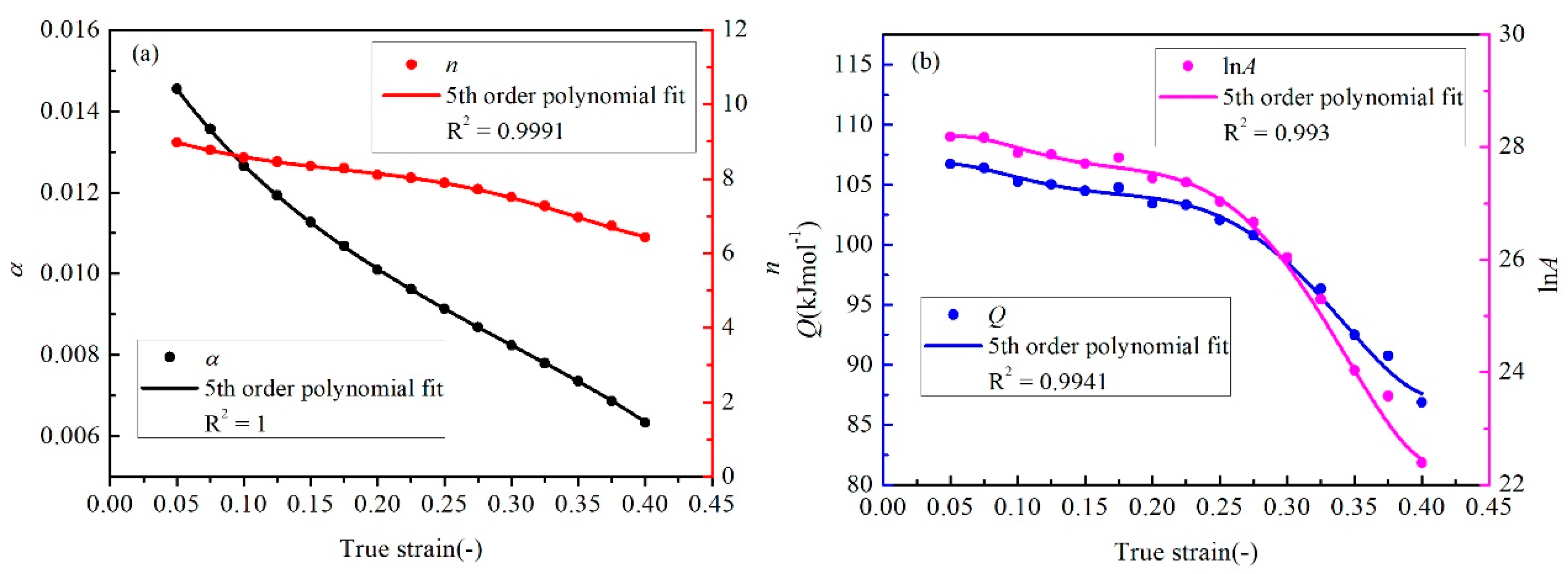
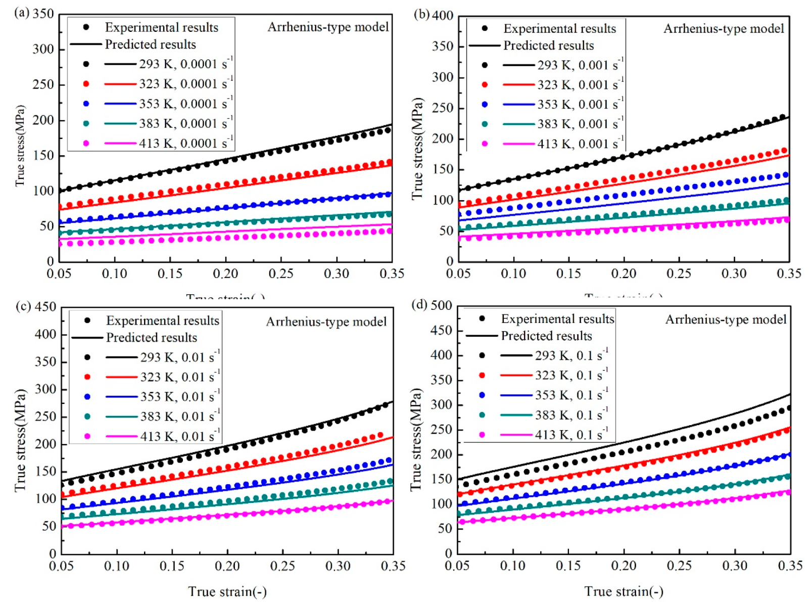
3.4. Arrhenius-Type Model
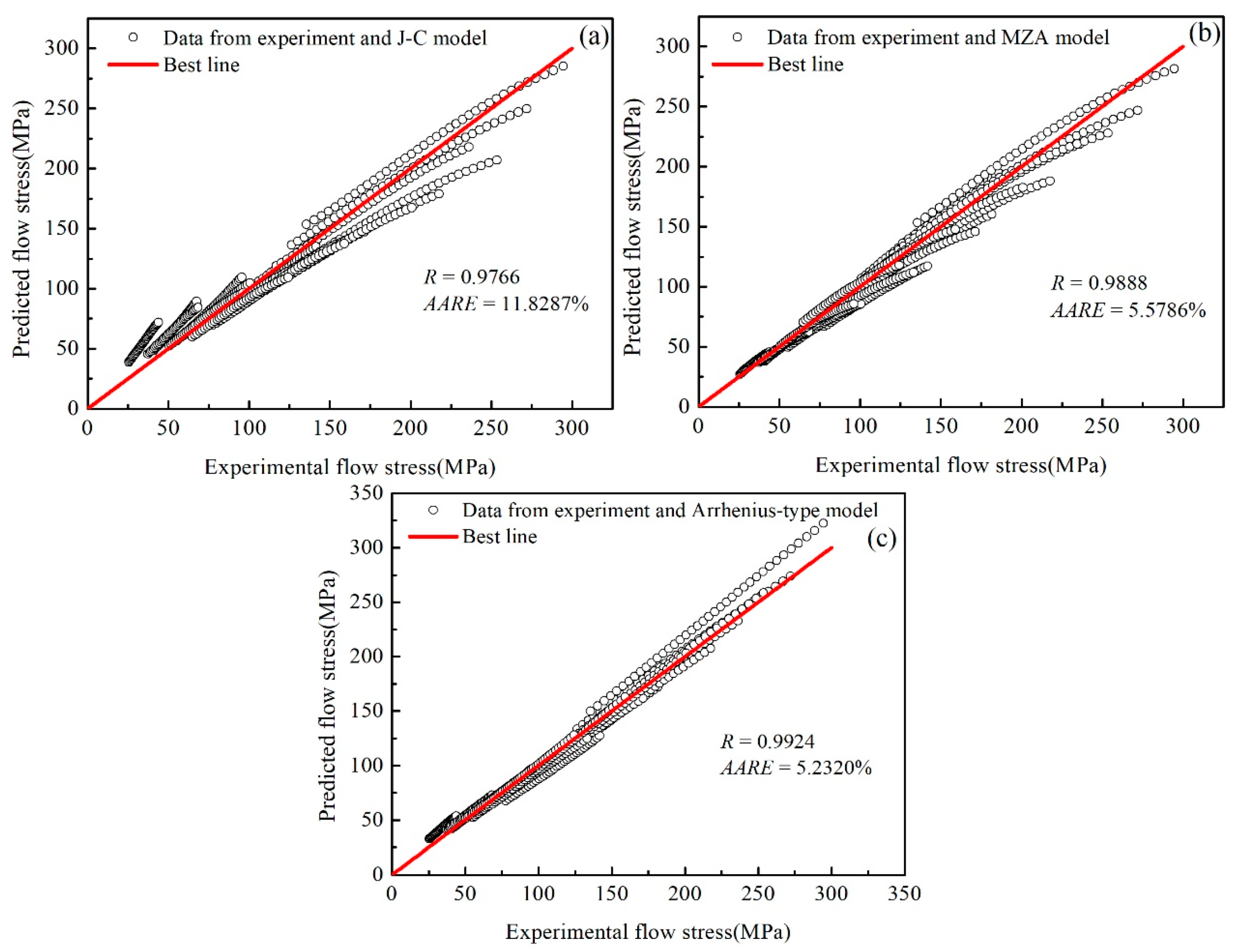
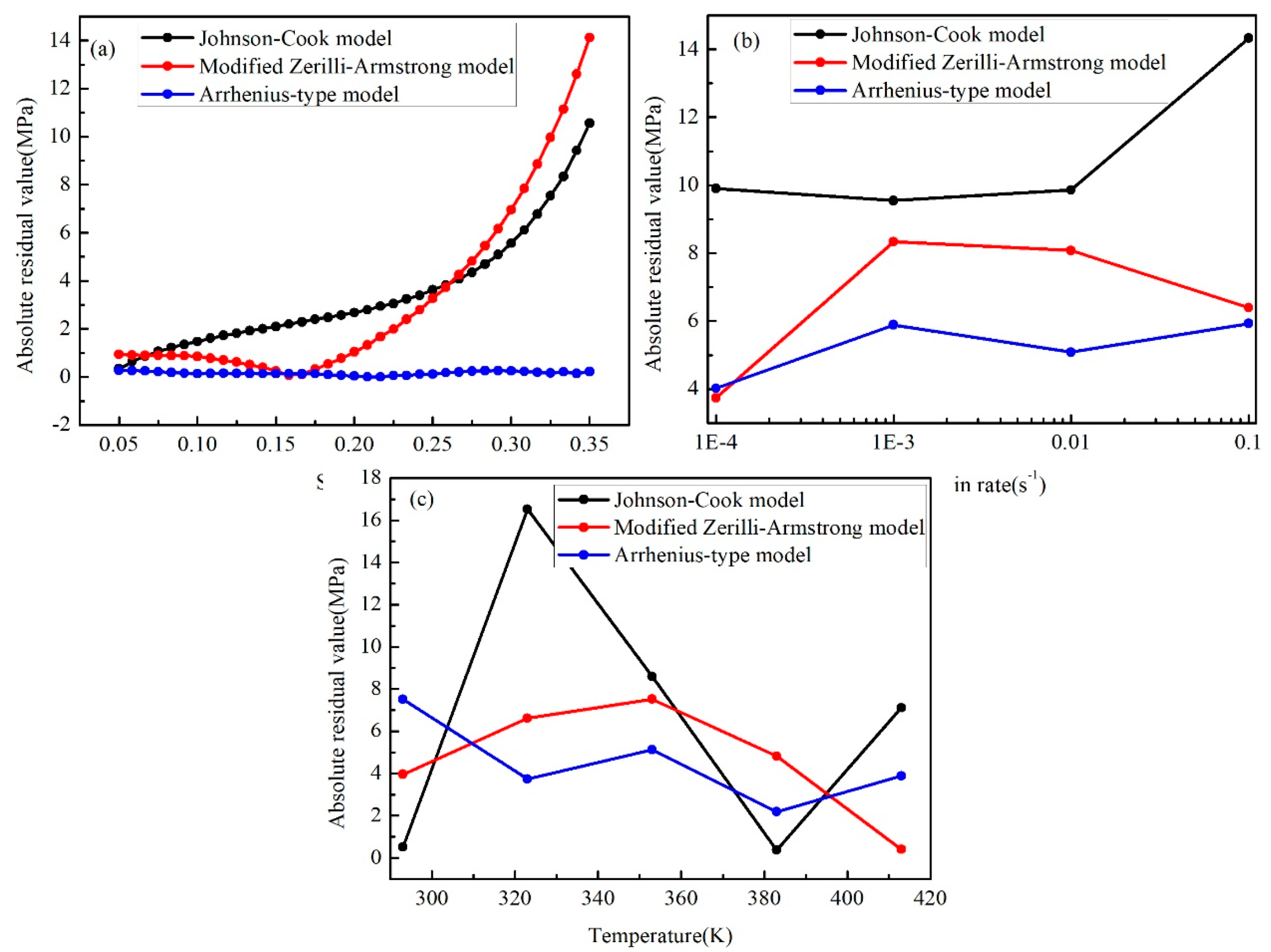
3.5. Accuracy Analysis
4. Conclusions
- The strain rate hardening effect and the temperature softening effect were notable for the flow behavior of the SnSbCu alloy.
- The J–C model could describe the flow behavior in the reference strain rate and temperature case, while, for other cases, the description was not effective since this model lacked the interaction of the strain rate hardening effect and the temperature softening effect.
- The prediction of the modified Z–A model could match the experimental results effectively at a low strain. However, the errors between experimental and predicted results enlarged with the increase of the strain.
- The A-type constitutive model can predict the flow behavior of the material under the whole focused range of temperatures and strain rates with the smallest errors and largest correlation coefficient among the three models, since the Zener–Hollomon parameter was employed to describe the interaction of the effect of the strain rate and the deformation.
Author Contributions
Funding
Acknowledgments
Conflicts of Interest
References
- El-Salam, F.A.; El-Khalek, A.M.A.; Nada, R.H.; Nagy, M.R.; EI-Haseeb, R.A. Thermally induced variations in structural and mechanical properties of rapid solidified Tin-based alloys. Mater. Sci. Eng. A 2009, 506, 135–140. [Google Scholar] [CrossRef]
- Bolotova, L.K.; Kalashnikov, I.E.; Kobeleva, L.I.; Bykov, P.A.; Katin, I.V.; Kolmakov, A.G.; Podymova, N.B. Structure and Properties of the B83 Babbit Alloy Based Composite Materials Produced by Extrusion. Inorg. Mater. Appl. Res. 2018, 9, 478–483. [Google Scholar] [CrossRef]
- Wang, J.M.; Xue, Y.W.; Li, W.H.; Wei, A.Z.; Cao, Y.F. Study on creep characteristics of oil film bearing Babbitt. Mater. Res. Innov. 2014, 18, S2-16–S2-21. [Google Scholar] [CrossRef]
- Wei, L.D.; Duan, S.L.; Xing, H.; Wu, J.; Wei, H.J. Thermo-elasto-hydroynamic behavior of main bearings of marine diesel engines in mixed lubrication. Trans. CSICE 2013, 31, 183–191. [Google Scholar]
- Wei, L.D.; Duan, S.L.; Wei, H.J. TEHD lubrication analysis of the main bearings of a marine diesel engine based on the flexible engine block. J. Harbin Eng. Univers. 2015, 36, 1035–1041. [Google Scholar]
- Wei, L.D.; Wei, H.J.; Duan, S.L.; Wu, Q.L.; Li, J.M. Thermo-elasto-hydroynamic mixed lubrication of marine bearings of marine diesel engines, based on coupling between flexible engine block and crankshaft. J. Mech. Eng. 2014, 50, 97–105. [Google Scholar] [CrossRef]
- Wei, L.D.; Wei, H.J.; Duan, S.L.; Zhang, Y. An EHD-mixed lubrication analysis of main bearings for diesel engine based on flexible whole engine block and crankshaft. Ind. Lubr. Tribol. 2015, 67, 150–158. [Google Scholar] [CrossRef]
- Xiang, G.; Han, Y.; Wang, J.; Xiao, K.; Li, J. A transient hydrodynamic lubrication comparative analysis for misaligned micro-grooved bearing considering axial reciprocating movement of shaft. Tribol. Int. 2019, 132, 11–23. [Google Scholar] [CrossRef]
- Gong, J.Y.; Jin, Y.; Liu, Z.L.; Jiang, H.; Xiao, M.H. Study on influencing factors of lubrication performance of water-lubricated micro-groove bearing. Tribol. Int. 2019, 129, 390–397. [Google Scholar] [CrossRef]
- Sarkar, S.; Golecha, K.; Kohli, S.; Kalmegh, A.; Yadav, S. Robust design of spiral groove journal bearing. SAE Int. J. Mater. Manuf. 2016, 9, 206–216. [Google Scholar] [CrossRef]
- Zhang, Y.; Zuo, T.T.; Tang, Z.; Gao, M.C.; Dahmen, K.A.; Liaw, P.K.; Lu, Z.P. Microstructures and properties of high-entropy alloys. Prog. Mater. Sci. 2014, 61, 1–93. [Google Scholar] [CrossRef]
- Gao, M.C.; Zhang, B.; Guo, S.M.; Qiao, J.W.; Hawk, J.A. High-entropy alloys in hexagonal close-packed structure. Metall. Mater. Trans. A 2016, 47, 3322–3332. [Google Scholar] [CrossRef]
- Miracle, D.B.; Senkov, O.N. A critical review of high entropy alloys and related concepts. Acta Mater. 2017, 122, 448–511. [Google Scholar] [CrossRef] [Green Version]
- Metasch, R.; Schwerz, R.; Roellig, M.; Kabakchiev, A.; Metais, B.; Ratchev, R.; Wolte, K.J. Experimental investigation on microstructural influence toward visco-plastic mechanical properties of Sn-based solder alloy for material modelling in Finite Element simulations. In Proceedings of the International Conference on Thermal, Budapest, Hungary, 19–22 April 2015. [Google Scholar]
- Gray, G.T.; Chen, S.R.; Vecchio, K.S. Influence of grain size on the constitutive response and substructure evolution of MONEL 400. Metall. Mater. Trans. A 1999, 30, 1235–1247. [Google Scholar] [CrossRef]
- Chiou, S.T.; Cheng, W.C.; Lee, W.S. Strain rate effects on the mechanical properties of a Fe–Mn–Al alloy under dynamic impact deformations. Mater. Sci. Eng. A 2005, 392, 156–162. [Google Scholar] [CrossRef]
- Choung, J.; Nam, W.; Lee, J.Y. Dynamic hardening behaviors of various marine structural steels considering dependencies on strain rate and temperature. Mar. Struct. 2013, 32, 49–67. [Google Scholar] [CrossRef]
- Johnson, G.R.; Cook, W.H. Fracture characteristics of three metals subjected to various strains, strain rates, temperatures and pressures. Eng. Fract. Mech. 1985, 21, 31–48. [Google Scholar] [CrossRef]
- Ashtiani, H.R.R.; Parsa, M.H.; Bisadi, H. Constitutive equations for elevated temperature flow behavior of commercial purity aluminum. Mater. Sci. Eng. A 2012, 545, 61–67. [Google Scholar] [CrossRef]
- Xu, G.F.; Peng, X.Y.; Liang, X.P.; Li, X.; Yin, Z.M. Constitutive relationship for high temperature deformation of Al-3Cu-0.5Sc alloy. Trans. Nonferr. Met. Soc. Chin. 2013, 23, 1549–1555. [Google Scholar] [CrossRef]
- Quan, G.Z.; Shi, Y.; Yu, C.T.; Zhou, J. The improved Arrhenius model with variable parameters of flow behavior characterizing for the as-cast AZ80 magnesium alloy. Mater. Res. 2013, 16, 785–791. [Google Scholar] [CrossRef]
- Zou, D.N.; Wu, K.; Han, Y.; Zhang, W.; Cheng, B.; Qiao, G.J. Deformation characteristic and prediction of flow stress for as-cast 21Cr economical duplex stainless steel under hot compression. Mater. Des. 2013, 51, 975–982. [Google Scholar] [CrossRef]
- Zerilli, F.J.; Armstrong, R.W. Dislocation-mechanics-based constitutive relations for material dynamics calculations. J. Appl. Phys. 1987, 61, 1816–1825. [Google Scholar] [CrossRef]
- Nasser, S.N.; Li, Y.L. Flow stress of fcc polycrystals with application to OFHC Cu. Acta Mater. 1998, 46, 565–577. [Google Scholar] [CrossRef]
- Jones, E.M.C.; Karlson, K.N.; Reu, P.L. Investigation of assumptions and approximations in the virtual fields method for a viscoplastic material model. Strain 2019. [Google Scholar] [CrossRef]
- Hu, Q.S.; Zhao, F.; Fu, H.; Li, K.W.; Liu, F.S. Dislocation density and mechanical threshold stress in OFHC copper subjected to SHPB loading and plate impact. Mater. Sci. Eng. A 2017, 695, 230–238. [Google Scholar] [CrossRef]
- Johnson, G.R.; Cook, W.H. A constitutive model and data for metals subjected to large strains, high strain rates, and high temperatures. In Proceedings of the Seventh International Symposium on Ballistics, International Ballistics Committee, Hague, Netherlands, 19–21 April 1983; pp. 541–547. [Google Scholar]
- Duan, C.Z.; Zhang, F.Y.; Qin, S.W.; Sun, W.; Wang, M.J. Modeling of dynamic recrystallization in white layer in dry hard cutting by finite element—cellular automaton method. J. Mech. Sci. Technol. 2018, 32, 4299–4312. [Google Scholar] [CrossRef]
- Laakso, S.V.; Niemi, E. Using FEM simulations of cutting for evaluating the performance of different johnson cook parameter sets acquired with inverse methods. Robot. Computer–Integr. Manuf. 2017, 47, 95–101. [Google Scholar] [CrossRef]
- Gurusamy, M.M.; Rao, B.C. On the performance of modified Zerilli-Armstrong constitutive model in simulating the metal-cutting process. J. Manuf. Process. 2017, 28, 253–265. [Google Scholar] [CrossRef]
- Paturi, U.M.R.; Narala, S.K.R.; Pundir, R.S. Constitutive flow stress formulation, model validation and FE cutting simulation for AA7075-T6 aluminum alloy. Mater. Sci. Eng. A 2014, 605, 176–185. [Google Scholar] [CrossRef]
- Khan, A.S.; Liu, J. A deformation mechanism based crystal plasticity model of ultrafine-grained/nanocrystalline FCC polycrystals. Int. J. Plast. 2016, 86, 56–69. [Google Scholar] [CrossRef]
- Anoop, A.D.; Sekhar, A.S.; Kamaraj, M.; Gopinath, K. Modelling the mechanical behaviour of heat-treated AISI 52100 bearing steel with retained austenite. Proc. IMechE Part L J. Mater. Des. Appl. 2018, 232, 44–57. [Google Scholar] [CrossRef]
- Kim, M.J.; Jeong, H.J.; Park, J.W.; Hong, S.T.; Han, H.N. Modified Johnson-Cook model incorporated with electroplasticity for uniaxial tension under a pulsed electric current. Met. Mater. Int. 2018, 24, 42–50. [Google Scholar] [CrossRef]
- He, J.L.; Chen, F.; Wang, B.; Zhu, L.B. A modified Johnson-Cook model for 10% Cr steel at elevated temperatures and a wide range of strain rates. Mater. Sci. Eng. A 2018, 715, 1–9. [Google Scholar] [CrossRef]
- Bobbili, R.; Madhu, V. A modified Johnson-Cook model for FeCoNiCr high entropy alloy over a wide range of strain rates. Mater. Lett. 2018, 218, 103–105. [Google Scholar] [CrossRef]
- Li, Z.X.; Zhan, M.; Fan, X.G.; Tan, J.Q. A modified Johnson-Cook model of as-quenched AA2219 considering negative to positive strain rate sensitivities over a wide temperature range. Proced. Eng. 2017, 207, 155–160. [Google Scholar] [CrossRef]
- Li, H.Y.; Wang, X.F.; Wei, D.D.; Hu, J.D.; Li, Y.H. A comparative study on modified Zerilli–Armstrong, Arrhenius-type and artificial neural network models to predict high-temperature deformation behavior in T24 steel. Mater. Sci. Eng. A 2012, 536, 216–222. [Google Scholar] [CrossRef]
- He, A.; Xie, G.L.; Zhang, H.L.; Wang, X.T. A comparative study on Johnson–Cook, modified Johnson–Cook and Arrhenius-type constitutive models to predict the high temperature flow stress in 20CrMo alloy steel. Mater. Des. 2013, 52, 677–685. [Google Scholar] [CrossRef]
- Li, J.; Li, F.G.; Cai, J.; Wang, R.T.; Yuan, Z.W.; Ji, G.L. Comparative investigation on the modified Zerilli–Armstrong model and Arrhenius-type model to predict the elevated-temperature flow behaviour of 7050 aluminium alloy. Comput. Mater. Sci. 2013, 71, 56–65. [Google Scholar] [CrossRef]
- Shrot, A.; Bäker, M. Determination of Johnson–Cook parameters from machining simulations. Comput. Mater. Sci. 2012, 52, 298–304. [Google Scholar] [CrossRef]
- Deng, X.G.; Hui, S.X.; Ye, W.J.; Song, X.Y. Construction of Johnson-Cook model for Gr2 Titanium through Adiabatic heating calculation. Appl. Mech. Mater. 2014, 487, 7–14. [Google Scholar] [CrossRef]
- Baghani, M.; Eskandari, A.H.; Zakerzadeh, M.R. Transient growth of a micro-void in an infinite medium under thermal load with modified Zerilli–Armstrong model. Acta Mech. 2016, 227, 943–953. [Google Scholar] [CrossRef]
- Mirzaie, T.; Mirzadeh, H.; Cabrera, J.M. A simple Zerilli–Armstrong constitutive equation for modeling and prediction of hot deformation flow stress of steels. Mech. Mater. 2016, 94, 38–45. [Google Scholar] [CrossRef]
- Lee, W.S.; Liu, C.Y. The effects of temperature and strain rate on the dynamic flow behaviour of different steels. Mater. Sci. Eng. A 2006, 426, 101–113. [Google Scholar] [CrossRef]
- Lin, Y.C.; Chen, M.S.; Zhong, J. Prediction of 42CrMo steel flow stress at high temperature and strain rate. Mech. Res. Commun. 2008, 35, 142–150. [Google Scholar] [CrossRef]
- Mandal, S.; Rakesh, V.; Sivaprasad, P.V.; Venugopal, S.; Kasiviswanathan, K.V. Constitutive equations to predict high-temperature flow stress in a Timodified austenitic stainless steel. Mater. Sci. Eng. A 2009, 500, 114–121. [Google Scholar] [CrossRef]
- Niu, X.Y.; Yu, Y.J.; Ma, L.H.; Chen, C. An Arrhenius-type constitutive model to predict the deformation behavior in lead-free solders. In Proceedings of the 2016 17th International Conference on Electronic Packaging Technology (ICEPT), Wuhan, China, 16–19 August 2016. [Google Scholar]
- Wang, W.; Zhao, J.; Zhai, R.X.; Ma, R. Arrhenius-Type Constitutive Model and Dynamic Recrystallization Behavior of 20Cr2Ni4A Alloy Carburizing Steel. Steel Res. Int. 2016, 88, 1600196. [Google Scholar] [CrossRef]
- Wang, L.; Liu, F.; Cheng, J.J.; Zuo, Q.; Chen, C.F. Arrhenius-Type Constitutive Model for High Temperature Flow Stress in a Nickel-Based Corrosion-Resistant Alloy. J. Mater. Eng. Perform. 2016, 25, 1394–1406. [Google Scholar] [CrossRef]
- Cai, J.; Li, F.G.; Liu, T.Y.; Chen, B.; He, M. Constitutive equations for elevated temperature flow stress of Ti-6Al-4V alloy considering the effect of strain. Mater. Des. 2011, 32, 1144–1151. [Google Scholar] [CrossRef]


| Strain (–) | I1 | S1 |
|---|---|---|
| 0.050 | 4.6752 | −0.01133 |
| 0.075 | 4.7444 | −0.01149 |
| 0.100 | 4.8044 | −0.01159 |
| 0.125 | 4.8626 | −0.01167 |
| 0.150 | 4.9166 | −0.01172 |
| 0.175 | 4.9691 | −0.01179 |
| 0.200 | 5.0184 | −0.01184 |
| 0.225 | 5.0653 | −0.01189 |
| 0.250 | 5.1106 | −0.01194 |
| 0.275 | 5.1535 | −0.01200 |
| 0.300 | 5.1951 | −0.01205 |
| 0.325 | 5.2365 | −0.01209 |
| 0.350 | 5.2785 | −0.01212 |
| 0.375 | 5.3243 | −0.01212 |
| 0.400 | 5.3738 | −0.01206 |
| α | n | Q(kJ/mol) | lnA |
|---|---|---|---|
| α0 = −0.9000 | n0 = +1433 | Q0 = +4.318 × 10⁴ | A0 = +1.332 × 10⁴ |
| α1 = +1.1240 | n1 = −1240 | Q1 = −4.375 × 10⁴ | A1 = −1.364 × 10⁴ |
| α2 = −0.6547 | n2 = +274.9 | Q2 = +1.537 × 10⁴ | A2 = +4880 |
| α3 = +0.2269 | n3 = +6.240 | Q3 = −2.353 × 10³ | A3 = −776.4 |
| α4 = −0.0619 | n4 = −11.46 | Q4 = +1.351 × 10² | A4 = +50.14 |
| α5 = +0.0172 | n5 = +9.510 | Q5 = +1.042 × 10² | A2 = +27.09 |
© 2019 by the authors. Licensee MDPI, Basel, Switzerland. This article is an open access article distributed under the terms and conditions of the Creative Commons Attribution (CC BY) license (http://creativecommons.org/licenses/by/4.0/).
Share and Cite
Li, T.; Zhao, B.; Lu, X.; Xu, H.; Zou, D. A Comparative Study on Johnson Cook, Modified Zerilli–Armstrong, and Arrhenius-Type Constitutive Models to Predict Compression Flow Behavior of SnSbCu Alloy. Materials 2019, 12, 1726. https://0-doi-org.brum.beds.ac.uk/10.3390/ma12101726
Li T, Zhao B, Lu X, Xu H, Zou D. A Comparative Study on Johnson Cook, Modified Zerilli–Armstrong, and Arrhenius-Type Constitutive Models to Predict Compression Flow Behavior of SnSbCu Alloy. Materials. 2019; 12(10):1726. https://0-doi-org.brum.beds.ac.uk/10.3390/ma12101726
Chicago/Turabian StyleLi, Tongyang, Bin Zhao, Xiqun Lu, Hanzhang Xu, and Dequan Zou. 2019. "A Comparative Study on Johnson Cook, Modified Zerilli–Armstrong, and Arrhenius-Type Constitutive Models to Predict Compression Flow Behavior of SnSbCu Alloy" Materials 12, no. 10: 1726. https://0-doi-org.brum.beds.ac.uk/10.3390/ma12101726