Application of the S-N Curve Mean Stress Correction Model in Terms of Fatigue Life Estimation for Random Torsional Loading for Selected Aluminum Alloys


Abstract
:1. Introduction
2. Materials
3. Methods
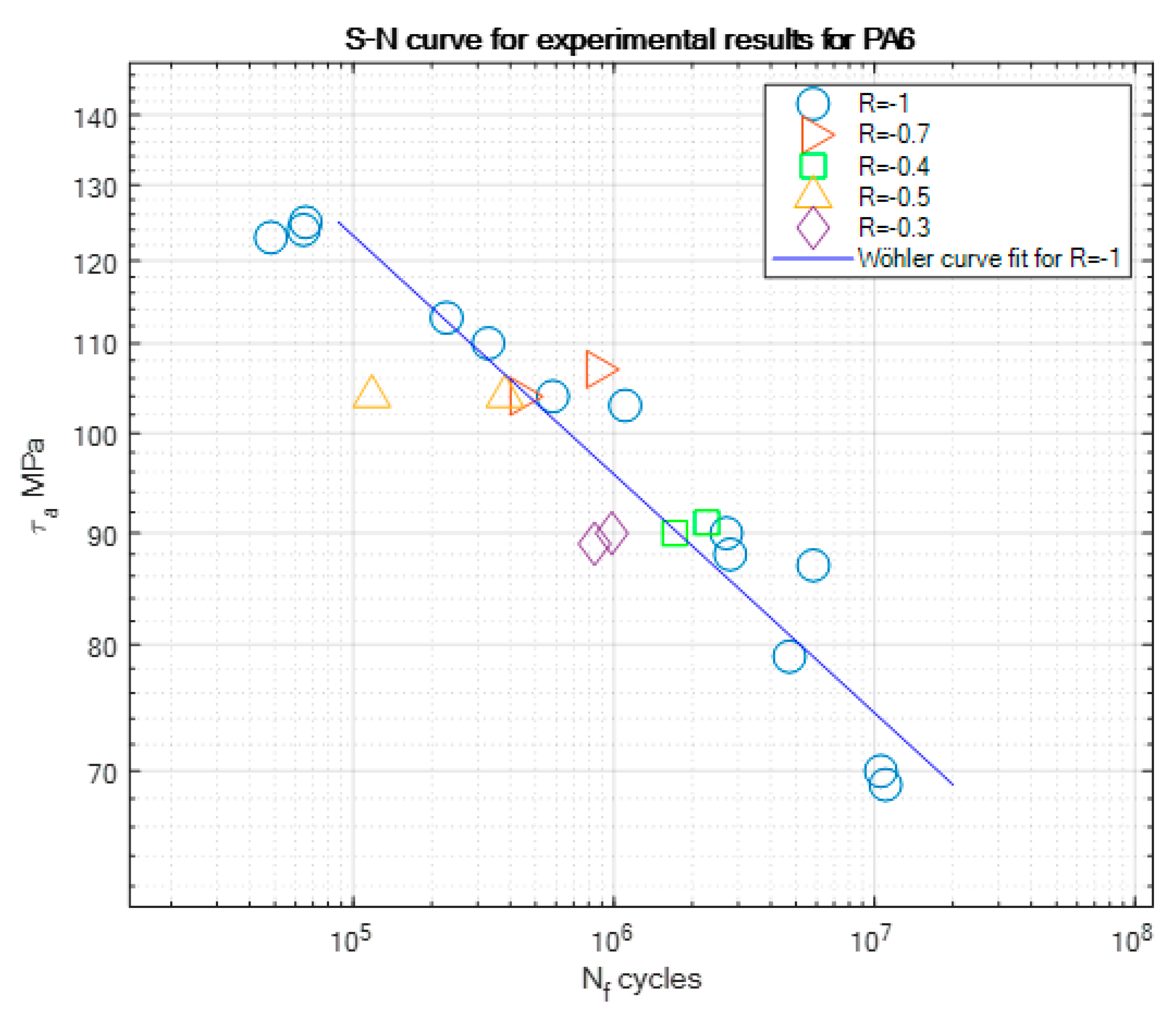
4. Results
5. Discussion
6. Conclusions and Observations
- The new design of the test samples has served its purpose, as it allowed us to obtain a pure shear distribution inside the sample.
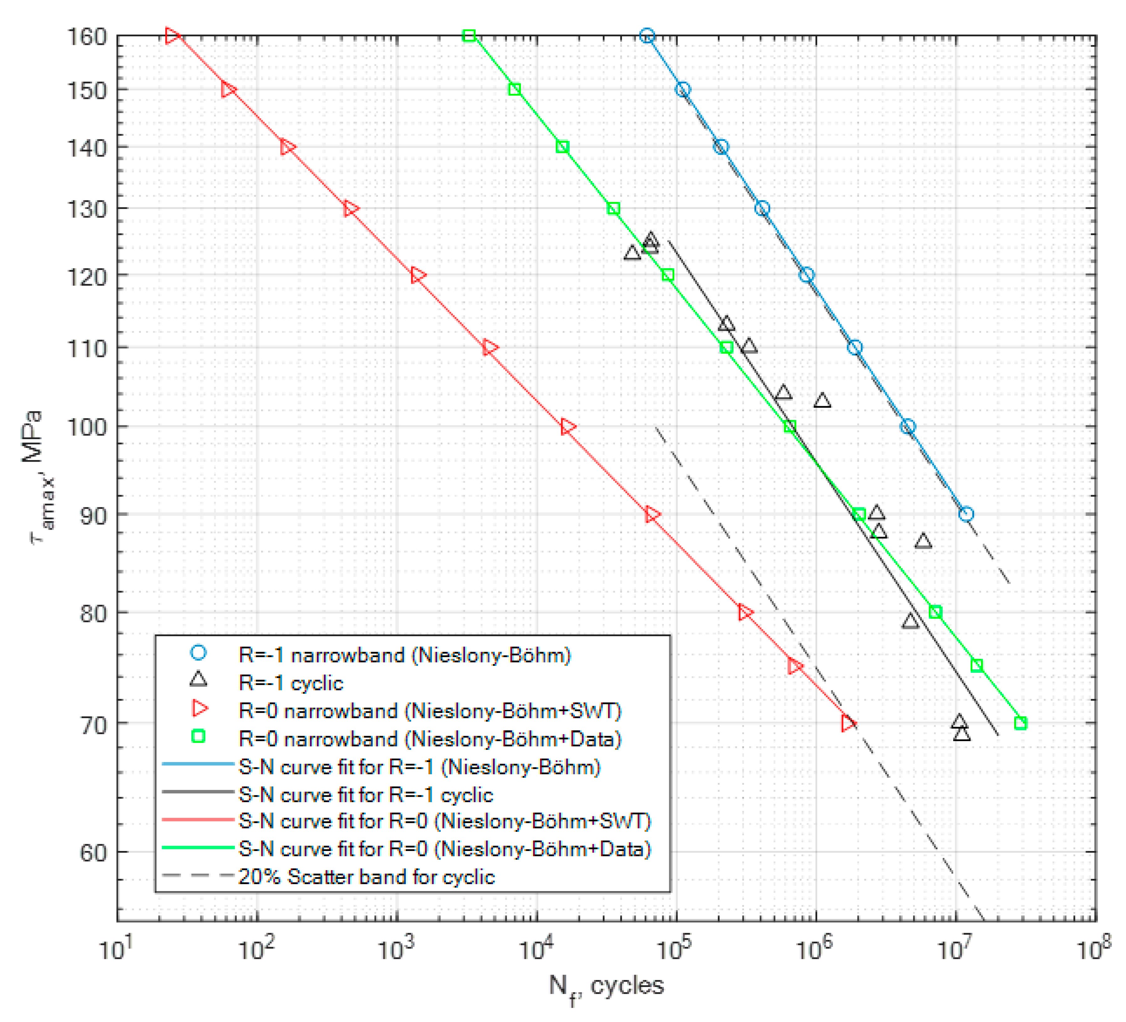
- The S-N curve Niesłony−Böhm (N-B) mean stress compensation model can also be applied to torsional loading conditions.
- The literature results for the missing fatigue strength amplitude for R = 0 used with the Niesłony−Böhm model have improved the results substantially in comparison to fatigue strengths obtained with the SWT model.
- The calculation results obtained for the generated narrowband loading signal have allowed us to perform calculations for three new S-N curves in the case of no mean stress correction for the ratio R = −1, and two mean stress effect compensations for R = 0 with different approaches to obtain the fatigue strength for the N−B model.
- It can be noted that the narrowband curves for R = 0 were within the scatter band of the cyclic results for R = −1, within or below the 20% area, whereas the calculation results for the narrowband curves for R = −1 were only in the scatter band of the PA6 alloy.
Author Contributions
Funding
Conflicts of Interest
References
- Wang, Q.; Zhang, W.; Jiang, S. Fatigue life prediction based on crack closure and equivalent initial flaw size. Materials 2015, 8, 7145–7160. [Google Scholar] [CrossRef] [PubMed] [Green Version]
- Zhang, J.; Li, W.; Dai, H.; Liu, N.; Lin, J. Study on the elastic–plastic correlation of low-cycle fatigue for variable asymmetric loadings. Materials 2020, 13, 2451. [Google Scholar] [CrossRef] [PubMed]
- Xing, Z.; Wang, Z.; Wang, H.; Shan, D. Bending fatigue behaviors analysis and fatigue life prediction of 20Cr2Ni4 gear steel with different stress concentrations near non-metallic inclusions. Materials 2019, 12, 3443. [Google Scholar] [CrossRef] [PubMed] [Green Version]
- Zhang, J.; Fu, X.; Lin, J.; Liu, Z.; Liu, N.; Wu, B. Study on damage accumulation and life prediction with loads below fatigue limit based on a modified nonlinear model. Materials 2018, 11, 2298. [Google Scholar] [CrossRef] [Green Version]
- Benasciutti, D.; Tovo, R. Frequenzbasierte analyse zufalliger ermudungsbelastungen: Modelle, hypothesen, praxis. Mater. Werkst. 2018, 49, 345–367. [Google Scholar] [CrossRef]
- Yu, Z.-Y.; Zhu, S.-P.; Liu, Q.; Liu, Y. Multiaxial fatigue damage parameter and life prediction without any additional material constants. Materials 2017, 10, 923. [Google Scholar] [CrossRef] [Green Version]
- Li, Y.; Hu, W.; Sun, Y.; Wang, Z.; Mosleh, A. A life prediction model of multilayered PTH based on fatigue mechanism. Materials 2017, 10, 382. [Google Scholar] [CrossRef] [Green Version]
- Xue, L.; Shang, D.G.; Li, L.J. Online fatigue damage evaluation method based on real-time cycle counting under multiaxial variable amplitude loading. IOP Conf. Ser. Mater. Sci. Eng. 2020, 784, 012014. [Google Scholar] [CrossRef]
- Zhu, S.-P.; Yue, P.; Yu, Z.-Y.; Wang, Q. A combined high and low cycle fatigue model for life prediction of turbine blades. Materials 2017, 10, 698. [Google Scholar] [CrossRef] [Green Version]
- Niesłony, A.; Böhm, M. Universal method for applying the mean-stress effect correction in stochastic fatigue-damage accumulation. MPC 2016, 5, 352–363. [Google Scholar] [CrossRef]
- Benasciutti, D.; Tovo, R. Spectral methods for lifetime prediction under wide-band stationary random processes. Int. J. Fatigue 2005, 27, 867–877. [Google Scholar] [CrossRef]
- Benasciutti, D. An analytical approach to measure the accuracy of various definitions of the “equivalent von Mises stress” in vibration multiaxial fatigue. In Proceedings of the International Conference on Engineering Vibration (ICoEV 2015), Ljubljana, Slovenia, 7–10 September 2015; pp. 743–752. [Google Scholar]
- Dirlik, T. Application of Computers in Fatigue Analysis. Ph.D. Thesis, University of Warwick, Coventry, UK, 1985. [Google Scholar]
- Rozumek, D.; Faszynka, S. Surface cracks growth in aluminum alloy AW-2017A-T4 under combined loadings. Eng. Fract. Mech. 2020, 226, 106896. [Google Scholar] [CrossRef]
- Kluger, K. Fatigue life estimation for 2017A-T4 and 6082-T6 aluminium alloys subjected to bending-torsion with mean stress. Int. J. Fatigue 2015, 80, 22–29. [Google Scholar] [CrossRef]
- Szusta, J.; Seweryn, A. Experimental study of the low-cycle fatigue life under multiaxial loading of aluminum alloy EN AW-2024-T3 at elevated temperatures. Int. J. Fatigue 2017, 96, 28–42. [Google Scholar] [CrossRef]
- Peč, M.; Zapletal, J.; Šebek, F.; Petruška, J. Low-cycle fatigue, fractography and life assessment of EN AW 2024-T351 under various loadings. Exp. Tech. 2019, 43, 41–56. [Google Scholar] [CrossRef]
- Gadolina, I.; Zaynetdinov, R. Advantages of the rain-flow method at the post-processing stage in comparison with the spectral approach. IOP Conf. Ser. Mater. Sci. Eng. 2019, 481, 012005. [Google Scholar] [CrossRef]
- Böhm, M.; Kowalski, M. Fatigue life assessment algorithm modification in terms of taking into account the effect of overloads in the frequency domain. AIP Conf. Proc. 2018, 2028, 020003. [Google Scholar] [CrossRef]
- Niesłony, A.; Böhm, M. Mean stress effect correction using constant stress ratio S–N curves. Int. J. Fatigue 2013, 52, 49–56. [Google Scholar] [CrossRef]
- Boller, C.; Seeger, T. Materials Data for Cyclic Loading; Elsevier: Amsterdam, The Netherlands, 1987; ISBN 978-0-444-42873-8. [Google Scholar]
- Goodman, J. Mechanics Applied to Engineering; Longmans, Green & Company: Harlow, UK, 1899. [Google Scholar]
- Gerber, W.Z. Bestimmung der zulässigen Spannungen in Eisen-Konstruktionen (Calculation of the allowable stresses in iron structures). Z. Bayer Arch. Ing. Ver. 1874, 6, 101–110. [Google Scholar]
- Soderberg, C. Factor of safety and working stress. Trans. ASME 1939, 52, 13–28. [Google Scholar]
- Morrow, J. Fatigue properties of metals. In Section 3.2, Fatigue Design Handbook; Society of Automotive Engineers: Warrendale, PA, USA, 1968; Volume AE-4. [Google Scholar]
- Zhu, S.-P.; Lei, Q.; Huang, H.-Z.; Yang, Y.-J.; Peng, W. Mean stress effect correction in strain energy-based fatigue life prediction of metals. Int. J. Damage Mech. 2016. [Google Scholar] [CrossRef]
- Tomčala, J.; Papuga, J.; Horák, D.; Hapla, V.; Pecha, M.; Čermák, M. Steps to increase practical applicability of PragTic software. Adv. Eng. Softw. 2019, 129, 57–68. [Google Scholar] [CrossRef]
- Gates, N.R.; Fatemi, A. Fatigue Life of 2024-T3 Aluminum under Variable Amplitude Multiaxial Loadings: Experimental Results and Predictions. Procedia Eng. 2015, 101, 159–168. [Google Scholar] [CrossRef] [Green Version]
- Wu, Z.-R.; Hu, X.-T.; Song, Y.-D. Multiaxial fatigue life prediction for titanium alloy TC4 under proportional and nonproportional loading. Int. J. Fatigue 2014, 59, 170–175. [Google Scholar] [CrossRef]
- Niezgodziński, M.E. Wzory, Wykresy i Tablice Wytrzymałościowe; Wydawnictwa Naukowo-Techniczne: Warsaw, Poland, 2007; ISBN 978-83-204-3380-7. [Google Scholar]
- Smith, K.; Watson, P.; Topper, T. A stress strain function for the fatigue of metals. J. Mater. ASTM 1970, 5, 767–778. [Google Scholar]
- Papuga, J.; Fojtík, F. Multiaxial fatigue strength of common structural steel and the response of some estimation methods. Int. J. Fatigue 2017, 104, 27–42. [Google Scholar] [CrossRef]
- Endo, T. Damage evaluation of metals for random on varying loading-three aspects of rain flow method. Mech. Behav. Mater. 1974, 1, 374. [Google Scholar]
- ASTM International. ASTM E1049-85 (2011) Practices for Cycle Counting in Fatigue Analysis; E08 Committee; ASTM International: West Conshohocken, PA, USA, 2011. [Google Scholar]
- Palmgren, A. Die lebensdauer von kugellagern. Z. Ver. Dtsch. Ing 1924, 14, 339–341. [Google Scholar]
- Nieslony, A.; Böhm, M. Determination of fatigue life on the basis of experimental fatigue diagrams under constant amplitude load with mean stress. In Fatigue Failure and Fracture Mechanics; Skibicki, D., Ed.; Trans Tech Publications Ltd: Stafa-Zurich, Switzerland, 2012; Volume 726, pp. 33–38. [Google Scholar]


| Standard | ||||
|---|---|---|---|---|
| PN | EN | WNR | ISO | DIN |
| PA4 | AW-6082-T6 | 3.2315 | AlSi1MgMn | AlMgSi1 |
| PA6 | AW-2017A-T4 | 3.1325 | AlCu4MgSi(A) | AlCuMg1 |
| PA7 | AW-2024-T3 | 3.1354 | AlCu4Mg1 | AlCuMg2 |
| Rm MPa | Re MPa | E MPa | υ | |
|---|---|---|---|---|
| PA4 | 344 ± 3 | 322 ± 2 | 69,000 | 0.33 |
| PA6 | 330 ± 2 | 312 ± 2 | 72,000 | 0.33 |
| PA7 | 497 | 359 | 73,200 | 0.33 |
| Fe | Si | Zn | Ti | Mg | Mn | Cu | Cr | Other | Al | |
|---|---|---|---|---|---|---|---|---|---|---|
| PA4 | 0.50 | 1.30 | 0.20 | 0.10 | 1.20 | 1 | 0.10 | 0.25 | 0.15 | balanced |
| PA6 | 0.70 | 0.80 | 0.25 | 0.25 | 1 | 1 | 4.50 | 0.10 | 0.15 | balanced |
| PA7 | 0.5 | 0.5 | 0.25 | 0.15 | 1.2 | 0.3 | 3.8 | 0.1 | 0.15 | balanced |
| Specimen No. | τm | τa | τmax | Nf |
|---|---|---|---|---|
| PA4-9 | 0 | 88 | 90 | 1,321,873 |
| PA4-14 | 0 | 91 | 90 | 1,848,426 |
| PA4-1 | 0 | 105 | 93 | 221,164 |
| PA4-8 | 0 | 104 | 104 | 457,156 |
| PA4-16 | 0 | 105 | 103 | 411,196 |
| PA4-2 | 0 | 121 | 119 | 174,696 |
| PA4-4 | 0 | 121 | 118 | 96,357 |
| PA4-3 | 0 | 137 | 131 | 21,409 |
| PA4-5 | 17 | 106 | 123 | 456,183 |
| PA4-10 | 19 | 106 | 125 | 230,671 |
| PA4-12 | 18 | 105 | 123 | 374,000 |
| PA4-6 | 35 | 88 | 122 | 1,700,497 |
| PA4-11 | 35 | 86 | 121 | 2,667,863 |
| PA4-13 | 37 | 89 | 126 | 2,048,000 |
| PA4-25 | 36 | 108 | 144 | 547,886 |
| PA4-26 | 35 | 105 | 140 | 464,294 |
| PA4-23 | 50 | 94 | 144 | 1,382,063 |
| PA4-24 | 49 | 97 | 146 | 1,905,095 |
| Specimen No. | τm | τa | τmax | Nf |
|---|---|---|---|---|
| PA6-12 | 0 | 70 | 71 | 10,567,970 |
| PA6-13 | 0 | 69 | 70 | 11,021,452 |
| PA6-9 | 0 | 79 | 81 | 4,714,524 |
| PA6-4 | 0 | 87 | 84 | 5,825,588 |
| PA6-5 | 0 | 88 | 87 | 2,793,997 |
| PA6-6 | 0 | 90 | 88 | 2,700,912 |
| PA6-10 | 0 | 103 | 105 | 1,104,340 |
| PA6-11 | 0 | 104 | 102 | 582,611 |
| PA6-7 | 0 | 113 | 111 | 227,991 |
| PA6-8 | 0 | 110 | 108 | 329,501 |
| PA6-1 | 0 | 125 | 119 | 65,574 |
| PA6-2 | 0 | 123 | 113 | 48,248 |
| PA6-3 | 0 | 124 | 114 | 64,380 |
| PA6-15 | 18 | 104 | 122 | 441,360 |
| PA6-16 | 17 | 107 | 124 | 864,694 |
| PA6-17 | 35 | 90 | 125 | 1,710,746 |
| PA6-18 | 37 | 91 | 127 | 2,273,590 |
| PA6-20 | 32 | 104 | 135 | 381,996 |
| PA6-21 | 29 | 104 | 133 | 117,770 |
| PA6-22 | 43 | 89 | 132 | 842,576 |
| PA6-23 | 46 | 90 | 136 | 981,805 |
| Specimen No. | τm | τa | τmax | Nf |
|---|---|---|---|---|
| PA7-13 | 0 | 60 | 58 | 11,035,860 |
| PA7-14 | 0 | 61 | 62 | 9,047,500 |
| PA7-10 | 0 | 71 | 72 | 3,119,563 |
| PA7-11 | 0 | 73 | 70 | 4,091,781 |
| PA7-8 | 0 | 88 | 91 | 2,514,519 |
| PA7-9 | 0 | 90 | 91 | 1,410,229 |
| PA7-4 | 0 | 105 | 105 | 993,766 |
| PA7-5 | 0 | 107 | 107 | 576,193 |
| PA7-7 | 0 | 104 | 103 | 827,959 |
| PA7-2 | 0 | 122 | 120 | 581,857 |
| PA7-6 | 0 | 126 | 125 | 332,553 |
| PA7-1 | 0 | 142 | 138 | 150,606 |
| PA7-3 | 0 | 146 | 145 | 113,728 |
| PA7-16 | 20 | 125 | 146 | 675,295 |
| PA7-17 | 20 | 125 | 146 | 511,227 |
| PA7-15 | 35 | 106 | 141 | 1,013,935 |
| PA7-18 | 34 | 105 | 139 | 684,876 |
| PA7-19 | 34 | 107 | 141 | 614,049 |
| PA7-20 | 34 | 120 | 154 | 359,856 |
| PA7-21 | 35 | 124 | 159 | 75,166 |
| PA7-22 | 58 | 107 | 166 | 459,271 |
| PA7-23 | 58 | 109 | 167 | 855,168 |
| m | τaf MPa | Nf Cycle | |
|---|---|---|---|
| PA4 | 9.25 | 90 | 1,848,426 |
| PA6 | 9.14 | 70 | 11,021,452 |
| PA7 | 4.69 | 60 | 11,035,860 |
| Material | SWT | Lit. Data |
|---|---|---|
| τafR = 0 MPa | τafR = 0 MPa | |
| PA4 | 63.64 | 76.5 |
| PA6 | 49.50 | 61.25 |
| PA7 | 42.43 | 49.8 |
| Material | SWT | Lit. Data |
|---|---|---|
| τafR=0/τaf | τafR=0/τaf | |
| PA4 | 0.707 | 0.85 |
| PA6 | 0.707 | 0.875 |
| PA7 | 0.707 | 0.83 |
© 2020 by the authors. Licensee MDPI, Basel, Switzerland. This article is an open access article distributed under the terms and conditions of the Creative Commons Attribution (CC BY) license (http://creativecommons.org/licenses/by/4.0/).
Share and Cite
Böhm, M.; Kluger, K.; Pochwała, S.; Kupina, M. Application of the S-N Curve Mean Stress Correction Model in Terms of Fatigue Life Estimation for Random Torsional Loading for Selected Aluminum Alloys. Materials 2020, 13, 2985. https://0-doi-org.brum.beds.ac.uk/10.3390/ma13132985
Böhm M, Kluger K, Pochwała S, Kupina M. Application of the S-N Curve Mean Stress Correction Model in Terms of Fatigue Life Estimation for Random Torsional Loading for Selected Aluminum Alloys. Materials. 2020; 13(13):2985. https://0-doi-org.brum.beds.ac.uk/10.3390/ma13132985
Chicago/Turabian StyleBöhm, Michał, Krzysztof Kluger, Sławomir Pochwała, and Mariusz Kupina. 2020. "Application of the S-N Curve Mean Stress Correction Model in Terms of Fatigue Life Estimation for Random Torsional Loading for Selected Aluminum Alloys" Materials 13, no. 13: 2985. https://0-doi-org.brum.beds.ac.uk/10.3390/ma13132985