
Integration of Fuzzy AHP and Fuzzy TOPSIS Methods for Wire Electric Discharge Machining of Titanium (Ti6Al4V) Alloy Using RSM

 ,
,  ,
,  ,
,  , , and
Abstract
:1. Introduction
2. Materials and Methods
2.1. Experimental Methodology
2.2. Fuzzy Analytical Hierarchy Process
- Step 1:
- Construct the various leveled structure of objective, criterion, and alternatives of the problem.
- Step 2:
- Construct a pairwise comparison matrix from the criteria/options available. Furthermore, assign linguistic terms using Figure 1 to the pairwise comparisons collected from decision makers. Convert linguistic terms into fuzzy numbers using Table 4. The generalized pairwise comparison matrix will be of the form shown in Equation (3).where = 1; i = j.
- Step 3:
- Fuzzification is used to convert the linguistic term into a membership term. The fuzzification of the linguistic term can be possible using various functions such as triangular, bell-shaped, and trapezoidal functions. For this study, we used the triangular membership function, as shown in Figure 2. The assumed fuzzy numbers are shown in Equations (4) and (5).where r, s, and t denote the lower, middle, and upper bounds of fuzzy number X, respectively, and l, m, and n denote the lower, middle, and the upper bounds of fuzzy number Y, respectively.Fuzzy weights can be found using fuzzy addition and multiplication [45]. The generalized fuzzy addition and fuzzy multiplication formulas are expressed by Equations (6) and (7).Fuzzy addition:Fuzzy multiplication:
- Step 4:
- Determine the fuzzy mean geometric value (FMGV) of each criteria using the geometric mean method. Equation (8) can be used for calculating FMGV. The fuzzy weights can be determined by using Equation (9).where is the comparison of fuzzy value from criterion i to j; is the geometric mean value for comparison of the fuzzy value of criterion j to every other criterion; is the fuzzy weight of each criterion.
2.3. Fuzzy TOPSIS
- Step 1:
- Normalization of response: The normalization is important for converting measured outputs into the fuzzy number. The process of normalization was carried out considering the output based on the benefit criteria or the cost criteria. The VC and MRR were normalized using the benefit criteria using Equation (10), whereas SR was normalized using the cost criteria using Equation (11).For benefit criteria:For cost criteria:where is the normalized value of output, is the maximum of and is the minimum of .
- Step 2:
- Fuzzification of normalized decision matrix: The decision matrix normalized in Step 1 can be converted to a fuzzified normalized decision matrix by assigning a sub-criteria grade to each alternative using Table 5 of the K membership function scale. Additionally, assign the weights to each sub-criteria grade.The weight of criteria:
- Step 3:
- Calculate the weighted normalized fuzzy decision matrix: The weights obtained from fuzzy AHP are required to construct this matrix. The weighted normalized values can be calculated as:
- Step 4:
- Identify the positive ideal (V+) and negative ideal (V−) solutions: The fuzzy positive ideal solutions (FPIS, V+) and the fuzzy negative ideal solutions (FNIS, V−) must be calculated using Equations (14) and (15)., where:, where:Consideration of the maximum and minimum of Vij does not necessarily result in triangular fuzzy numbers, but we can obtain the ideal solutions as the fuzzy numbers using Equation (16).where = (, ) and = ().
- Step 5:
- Calculate separation measures: The separation measure is the summation of the distance of each response to the FPIS and is the summation of the distance of each response to the FNIS. The distance can be calculated by using the following equations.
- Step 6:
- Calculate the similarities to the ideal solution: To solve the similarities, compute the closeness coefficient CCi for each alternative [48].
3. Results and Discussions
3.1. Regression Equations
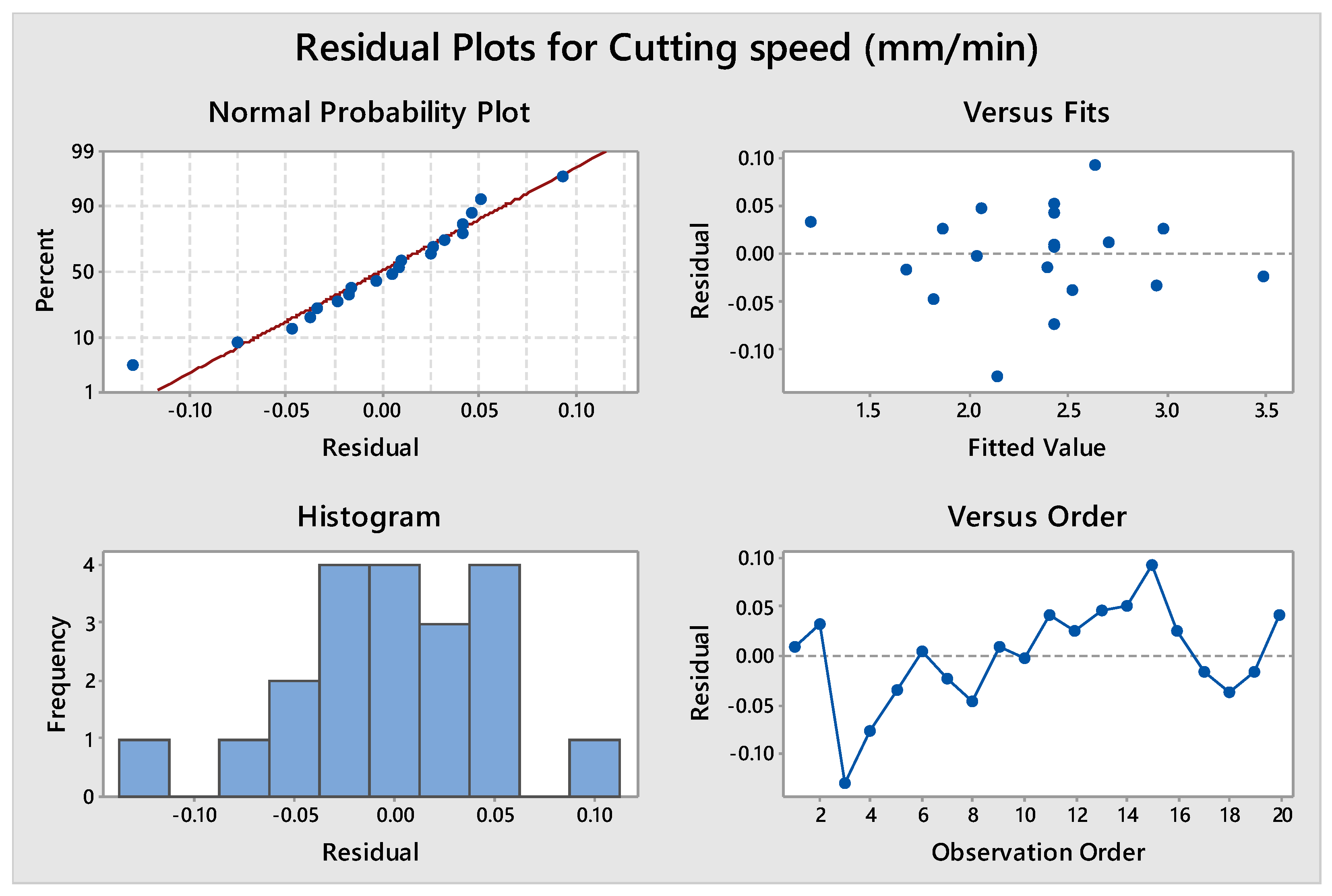
3.2. Analysis of Cutting Speed
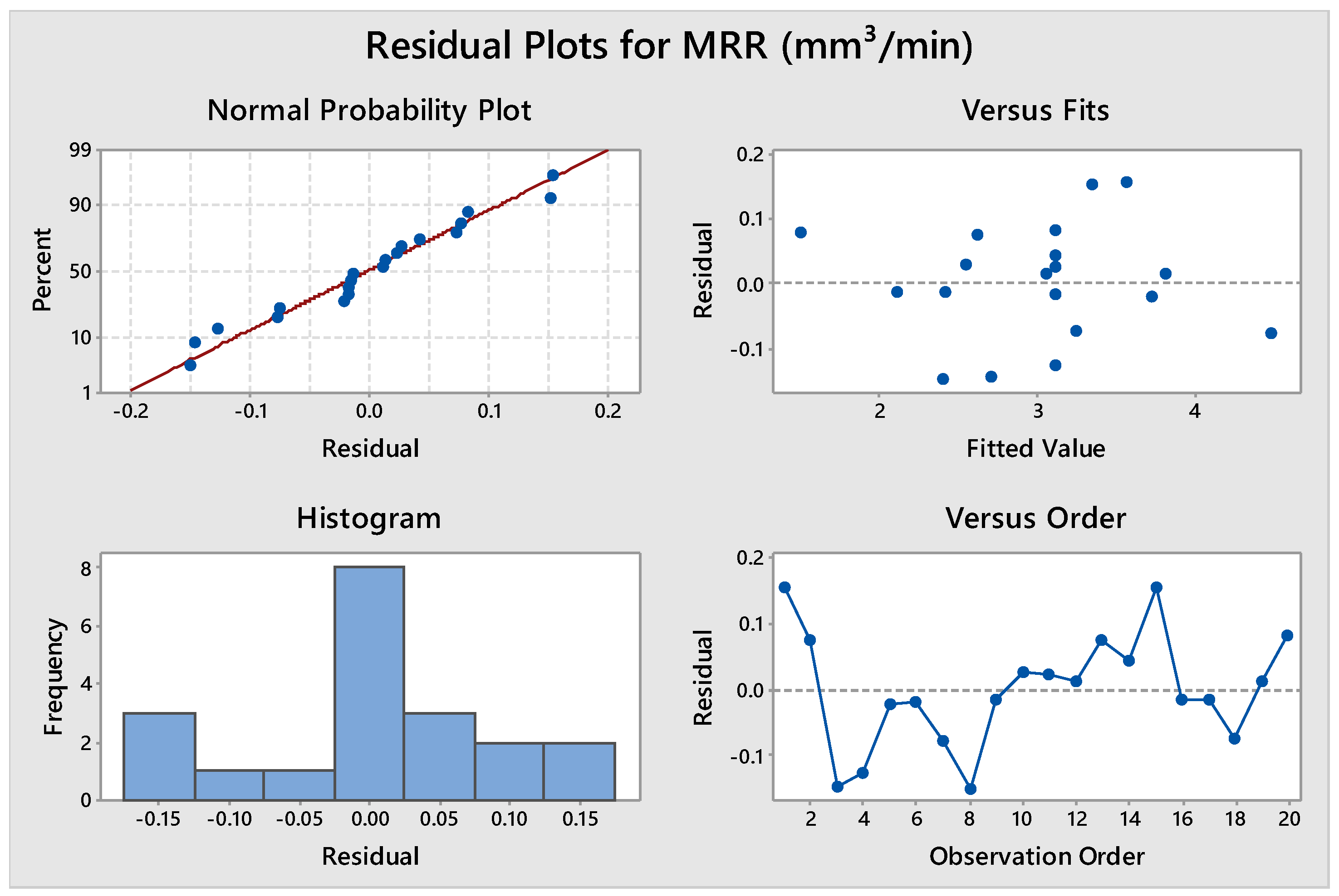
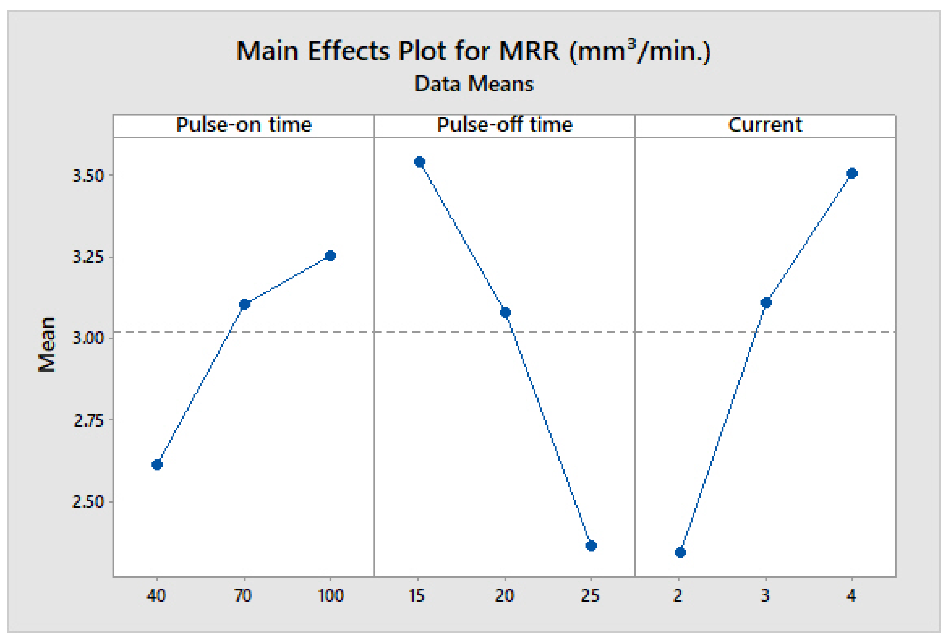
3.3. Analysis of MRR
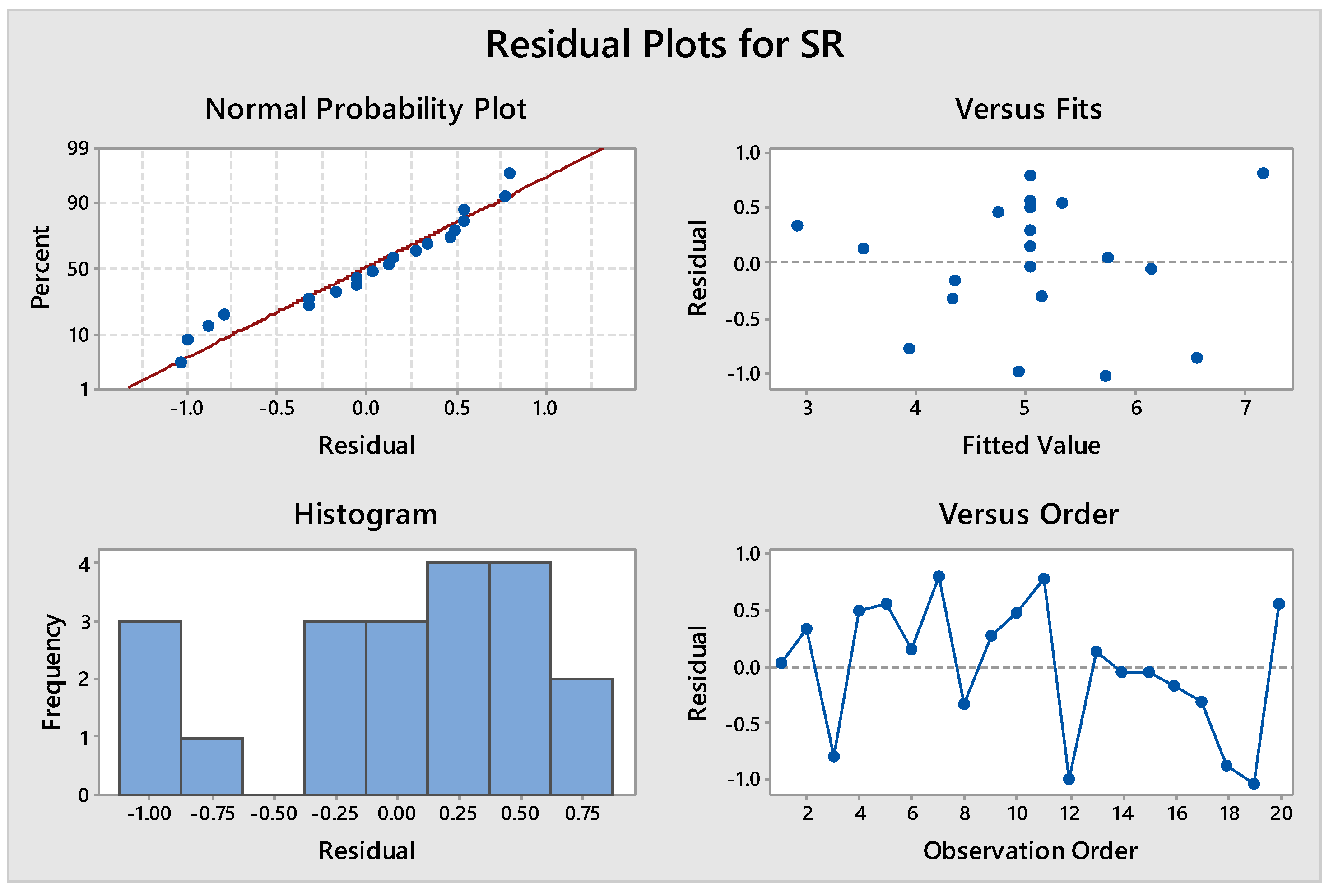
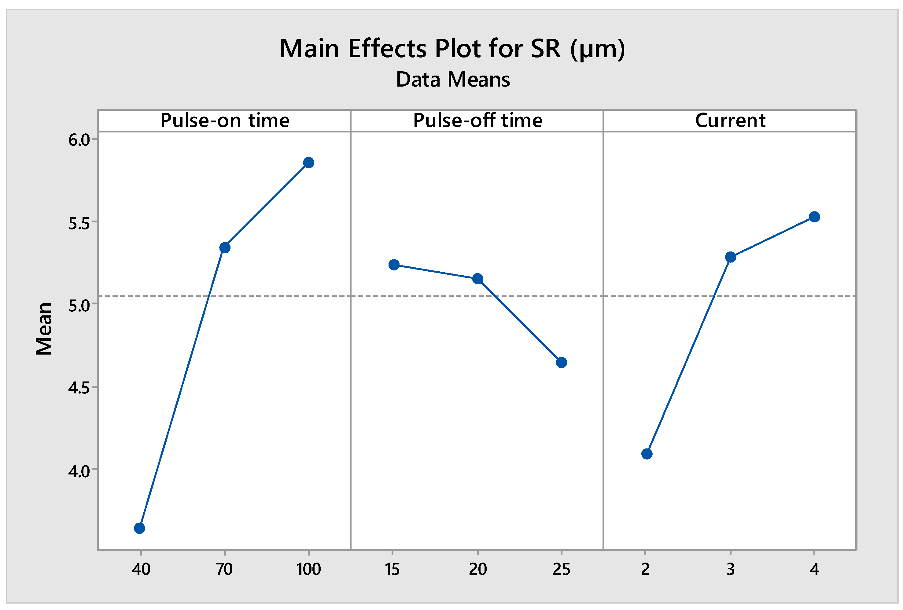
3.4. Analysis of SR
3.5. Optimization Using Integrated Fuzzy AHP and Fuzzy TOPSIS
3.5.1. Fuzzy AHP
3.5.2. Fuzzy TOPSIS
4. Conclusions
- Response surface methodology is effective for systematically designing the experiments. The mathematical relations developed between dependent and independent parameters are significant for predicting the responses at a 95% confidence interval.
- ANOVA analysis confirmed that the input parameters Ton, Toff, and current significantly affect cutting speed, material removal rate, and surface roughness.
- Fuzzy AHP can be incorporated to prioritize the responses using data collected from experts. The use of the fuzzy approach eliminates the aleatory uncertainty present in the natural language. The weights calculated using fuzzy AHP can be incorporated in fuzzy TOPSIS without bias.
- For the considered range of process parameters, the optimal process parameters for WEDM are Ton = 40 µs, Toff = 15 µs, and current = 2A.
- The confirmatory experiments proved that fuzzy logic is an effective and efficient solution for the optimization of WEDM process parameters. The proposed integrated approach of RSM, fuzzy AHP, and fuzzy TOPSIS can be further extended for different machining processes.
Author Contributions
Funding
Institutional Review Board Statement
Informed Consent Statement
Data Availability Statement
Conflicts of Interest
Nomenclature
| AHP | Analytical hierarchy process |
| ANOVA | Analysis of variance |
| CCi | Closeness coefficient index |
| CCD | Central composite design |
| CR | Consistency ratio |
| FMGV | Fuzzy mean geometric value |
| FPIS | Fuzzy positive ideal solutions |
| FNIS | Fuzzy negative ideal solutions |
| GRA | Gray relational analysis |
| HTS | Heat transfer search |
| MCDM | Multi-criteria decision making |
| MRR | Material removal rate |
| RSM | Response surface methodology |
| S/N | Single to noise |
| SR | Surface roughness |
| TOPSIS | Technique for Order Preference by Similarity to Ideal Solution |
| Ton | Pulse-on time |
| Toff | Pulse-off time |
| VC | Cutting speed |
| WF | Wire feed rate |
| WEDM | Wire electrical discharge machining process |
References
- Ezugwu, E.; Wang, Z. Titanium alloys and their machinability—A review. J. Mater. Process. Technol. 1997, 68, 262–274. [Google Scholar] [CrossRef]
- Chaudhari, R.; Vora, J.J.; Prabu, S.M.; Palani, I.; Patel, V.K.; Parikh, D. Pareto optimization of WEDM process parameters for machining a NiTi shape memory alloy using a combined approach of RSM and heat transfer search algorithm. Adv. Manuf. 2019, 9, 64–80. [Google Scholar] [CrossRef]
- Baltatu, M.S.; Vizureanu, P.; Sandu, A.V.; Florido-Suarez, N.; Saceleanu, M.V.; Mirza-Rosca, J.C.J.M. New Titanium Alloys. Promis. Mater. Med Devices 2021, 14, 5934. [Google Scholar]
- Nicholson, J.J.P.W. Titanium alloys for dental implants: A review. Prosthesis 2020, 2, 100–116. [Google Scholar] [CrossRef]
- Saravanan, R.; Rani, M.P. Metal and Alloy Bonding—An Experimental Analysis: Charge Density in Metals and Alloys; Springer Science & Business Media: Berlin/Heidelberg, Germany, 2011. [Google Scholar]
- Vora, J.; Chaudhari, R.; Patel, C.; Pimenov, D.Y.; Patel, V.K.; Giasin, K.; Sharma, S. Experimental Investigations and Pareto Optimization of Fiber Laser Cutting Process of Ti6Al4V. Metals 2021, 11, 1461. [Google Scholar] [CrossRef]
- Hourmand, M.; Sarhan, A.A.; Sayuti, M.; Hamdi, M.J.A. A Comprehensive Review on Machining of Titanium Alloys. Engineering 2021, 1–37. [Google Scholar] [CrossRef]
- Chaudhari, R.; Vora, J.; Parikh, D.; Wankhede, V.; Khanna, S. Multi-response Optimization of WEDM Parameters Using an Integrated Approach of RSM–GRA Analysis for Pure Titanium. J. Inst. Eng. Ser. D 2020, 101, 117–126. [Google Scholar] [CrossRef]
- Gupta, V.; Singh, B.; Mishra, R.K. Machining of titanium and titanium alloys by electric discharge machining process: A review. Int. J. Mach. Mach. Mater. 2020, 22, 99–121. [Google Scholar]
- Chaudhari, R.; Vora, J.J.; Pramanik, A.; Parikh, D. Optimization of Parameters of Spark Erosion Based Processes. Spark Erosion Machining; CRC Press: Boca Raton, FL, USA, 2020; pp. 190–216. [Google Scholar]
- Sheth, M.; Gajjar, K.; Jain, A.; Shah, V.; Patel, H.; Chaudhari, R.; Vora, J. Multi-objective optimization of inconel 718 using Combined approach of taguchi—Grey relational analysis. In Advances in Mechanical Engineering; Springer: Singapore, 2021; pp. 229–235. [Google Scholar]
- Joshi, R.; Zinzala, G.; Nirmal, N.; Fuse, K. Multi-Response Optimization of EDM for Ti-6Al-4V Using Taguchi-Grey Relational Analysis. Solid State Phenomena; Trans Tech Publications Ltd.: Bäch, Switzerland, 2017. [Google Scholar]
- Aggarwal, V.; Pruncu, C.I.; Singh, J.; Sharma, S.; Pimenov, D.Y.J.M. Empirical investigations during WEDM of Ni-27Cu-3.15 Al-2Fe-1.5 Mn based superalloy for high temperature corrosion resistance applications. Materials 2020, 13, 3470. [Google Scholar] [CrossRef]
- Sen, B.; Hussain, S.A.I.; Gupta, A.D.; Gupta, M.K.; Pimenov, D.Y.; Mikołajczyk, T.J.M. Application of Type-2 Fuzzy AHP-ARAS for Selecting Optimal WEDM Parameters. Metals 2021, 11, 42. [Google Scholar] [CrossRef]
- Rathi, P.; Ghiya, R.; Shah, H.; Srivastava, P.; Patel, S.; Chaudhari, R.; Vora, J. Multi-Response Optimization of Ni55. 8Ti Shape Memory Alloy Using Taguchi–Grey Relational Analysis Approach. Recent Advances in Mechanical Infrastructure; Springer: Singapore, 2020; pp. 13–23. [Google Scholar]
- Goyal, A. Investigation of material removal rate and surface roughness during wire electrical discharge machining (WEDM) of Inconel 625 super alloy by cryogenic treated tool electrode. J. King Saud Univ.-Sci. 2017, 29, 528–535. [Google Scholar] [CrossRef]
- Lenin, N.; Sivakumar, M.; Selvakumar, G.; Rajamani, D.; Sivalingam, V.; Gupta, M.K.; Mikolajczyk, T.; Pimenov, D.Y. Optimization of Process Control Parameters for WEDM of Al-LM25/Fly Ash/B4C Hybrid Composites Using Evolutionary Algorithms: A Comparative Study. Metals 2021, 11, 1105. [Google Scholar] [CrossRef]
- Patel, S.; Fuse, K.; Gangvekar, K.; Badheka, V. Multi-response optimization of dissimilar Al-Ti alloy FSW using Taguchi-Grey relational analysis. In Key Engineering Materials; Trans Tech Publications Ltd.: Bäch, Switzerland, 2020. [Google Scholar]
- Vora, J.; Patel, V.K.; Srinivasan, S.; Chaudhari, R.; Pimenov, D.Y.; Giasin, K.; Sharma, S. Optimization of Activated Tungsten Inert Gas Welding Process Parameters Using Heat Transfer Search Algorithm: With Experimental Validation Using Case Studies. Metals 2021, 11, 981. [Google Scholar] [CrossRef]
- Chaudhari, R.; Khanna, S.; Vora, J.; Patel, V.K.; Paneliya, S.; Pimenov, D.Y.; Wojciechowski, S. Experimental investigations and optimization of MWCNTs-mixed WEDM process parameters of nitinol shape memory alloy. J. Mater. Res. Technol. 2021, 15, 2152–2169. [Google Scholar] [CrossRef]
- Nain, S.S.; Garg, D.; Kumar, S. Investigation for obtaining the optimal solution for improving the performance of WEDM of super alloy Udimet-L605 using particle swarm optimization. Eng. Sci. Technol. Int. J. 2018, 21, 261–273. [Google Scholar] [CrossRef]
- Sharma, N.; Khanna, R.; Gupta, R.D. WEDM process variables investigation for HSLA by response surface methodology and genetic algorithm. Eng. Sci. Technol. Int. J. 2015, 18, 171–177. [Google Scholar] [CrossRef] [Green Version]
- Phate, M.R.; Toney, S.B. Modeling and prediction of WEDM performance parameters for Al/SiCp MMC using dimensional analysis and artificial neural network. Eng. Sci. Technol. Int. J. 2019, 22, 468–476. [Google Scholar] [CrossRef]
- Sharma, N.; Khanna, R.; Gupta, R.D.; Sharma, R. Modeling and multiresponse optimization on WEDM for HSLA by RSM. Int. J. Adv. Manuf. Technol. 2013, 67, 2269–2281. [Google Scholar] [CrossRef]
- Kavimani, V.; Prakash, K.S.; Thankachan, T. Multi-objective optimization in WEDM process of graphene–SiC-magnesium composite through hybrid techniques. Measurement 2019, 145, 335–349. [Google Scholar] [CrossRef]
- Bose, S.; Nandi, T. A novel optimization algorithm on surface roughness of WEDM on titanium hybrid composite. Sādhanā 2020, 45, 236. [Google Scholar] [CrossRef]
- Daniel, G.; Kumar, P.M. Parametric study and optimization of regression model in WEDM using genetic algorithm. IOP Conf. Ser. Mater. Sci. Eng. 2020, 764, 012047. [Google Scholar] [CrossRef]
- Prasad Arikatla, S.; Tamil Mannan, K.; Krishnaiah, A. Parametric Optimization in Wire Electrical Discharge Machining of Titanium Alloy Using Response Surface Methodology. Mater. Today Proc. 2017, 4, 1434–1441. [Google Scholar] [CrossRef]
- Chaudhari, R.; Vora, J.J.; Mani Prabu, S.S.; Palani, I.A.; Patel, V.K.; Parikh, D.M.; de Lacalle, L.N.L. Multi-Response Optimization of WEDM Process Parameters for Machining of Superelastic Nitinol Shape-Memory Alloy Using a Heat-Transfer Search Algorithm. Materials 2019, 12, 1277. [Google Scholar] [CrossRef] [Green Version]
- Saedon, J.; Jaafar, N.; Yahaya, M.A.; Nor, N.M.; Husain, H. A study on kerf and material removal rate in wire electricaldischarge machining of Ti-6Al-4V: Multi-objectives optimization. In Proceedings of the 2014 2nd International Conference on Technology, Informatics, Management, Engineering & Environment, Bandung, Indonesia, 19–21 August 2014. [Google Scholar]
- Payal, H.; Maheshwari, S.; Bharti, P.S.; Sharma, S.K. Multi-objective optimisation of electrical discharge machining for Inconel 825 using Taguchi-fuzzy approach. Int. J. Inf. Technol. 2019, 11, 97–105. [Google Scholar] [CrossRef]
- Modi, D.; Dalsaniya, A.; Fuse, K.; Kanakhara, M. Optimizing the Design of Brake Disc Using Multi-criteria Decision-making Method AHP-TOPSIS for All-terrain Vehicle. In Proceedings of the 2020 9th International Conference on Industrial Technology and Management (ICITM), Oxford, UK, 1–13 February 2020. [Google Scholar]
- Ananthakumar, K.; Rajamani, D.; Balasubramanian, E.; Davim, J.P. Measurement and optimization of multi-response characteristics in plasma arc cutting of Monel 400™ using RSM and TOPSIS. Measurement 2019, 135, 725–737. [Google Scholar] [CrossRef]
- Prabhu, S.R.; Shettigar, A.; Herbert, M.; Rao, S. Multi response optimization of friction stir welding process variables using TOPSIS approach. IOP Conf. Ser. Mater. Sci. Eng. 2018, 376, 012134. [Google Scholar] [CrossRef] [Green Version]
- Tamjidy, M.; Baharudin, B.; Paslar, S.; Matori, K.; Sulaiman, S.; Fadaeifard, F. Multi-objective optimization of friction stir welding process parameters of AA6061-T6 and AA7075-T6 using a biogeography based optimization algorithm. Materials 2017, 10, 533. [Google Scholar] [CrossRef] [Green Version]
- Sudhagar, S.; Sakthivel, M.; Mathew, P.J.; Daniel, S.A.A. A multi criteria decision making approach for process improvement in friction stir welding of aluminium alloy. Measurement 2017, 108, 1–8. [Google Scholar] [CrossRef]
- Gaidhani, Y.; Kalamani, V. Abrasive water jet review and parameter selection by AHP method. IOSR J. Mech. Civil. Eng. 2013, 8, 1–6. [Google Scholar] [CrossRef]
- Babu, K.A.; Venkataramaiah, P. Multi-response optimization in wire electrical discharge machining (WEDM) of Al6061/SiCp composite using hybrid approach. J. Manuf. Sci. Prod. 2015, 15, 327–338. [Google Scholar]
- Nayak, B.; Mahapatra, S. Multi-response optimization of WEDM process parameters using the AHP and TOPSIS method. Int. J. Theor. Appl. Res. Mech. Eng. 2013, 2, 109–215. [Google Scholar]
- Chou, Y.-C.; Yen, H.-Y.; Dang, V.T.; Sun, C.-C. Assessing the Human Resource in Science and Technology for Asian Countries: Application of Fuzzy AHP and Fuzzy TOPSIS. Symmetry 2019, 11, 251. [Google Scholar] [CrossRef] [Green Version]
- Sirisawat, P.; Kiatcharoenpol, T. Fuzzy AHP-TOPSIS approaches to prioritizing solutions for reverse logistics barriers. Comput. Ind. Eng. 2018, 117, 303–318. [Google Scholar] [CrossRef]
- Roy, T.; Dutta, R.K. Integrated fuzzy AHP and fuzzy TOPSIS methods for multi-objective optimization of electro discharge machining process. Soft Comput. 2019, 23, 5053–5063. [Google Scholar] [CrossRef]
- Saaty, T.L. A scaling method for priorities in hierarchical structures. J. Math. Psychol. 1977, 15, 234–281. [Google Scholar] [CrossRef]
- Wijitkosum, S.; Sriburi, T. Fuzzy AHP integrated with GIS analyses for drought risk assessment: A case study from upper Phetchaburi River basin, Thailand. Water 2019, 11, 939. [Google Scholar] [CrossRef] [Green Version]
- Leśniak, A.; Kubek, D.; Plebankiewicz, E.; Zima, K.; Belniak, S. Fuzzy AHP application for supporting contractors’ bidding decision. Symmetry 2018, 10, 642. [Google Scholar] [CrossRef] [Green Version]
- Chen, S.-J.; Hwang, C.-L. Fuzzy Multiple Attribute Decision Making Methods. Fuzzy Multiple Attribute Decision Making; Springer: Berlin, Germany, 1992; pp. 289–486. [Google Scholar]
- Nădăban, S.; Dzitac, S.; Dzitac, I. Fuzzy TOPSIS: A General View. Procedia Comput. Sci. 2016, 91, 823–831. [Google Scholar] [CrossRef] [Green Version]
- Chen, C.-T.; Lin, C.-T.; Huang, S.-F. A fuzzy approach for supplier evaluation and selection in supply chain management. Int. J. Prod. Econ. 2006, 102, 289–301. [Google Scholar] [CrossRef]
- Torfi, F.; Farahani, R.Z.; Rezapour, S. Fuzzy AHP to determine the relative weights of evaluation criteria and Fuzzy TOPSIS to rank the alternatives. Appl. Soft Comput. 2010, 10, 520–528. [Google Scholar] [CrossRef]
- Chaudhari, R.; Vora, J.J.; Patel, V.; López de Lacalle, L.; Parikh, D.J.M. Surface analysis of wire-electrical-discharge-machining-processed shape-memory alloys. Materials 2020, 13, 530. [Google Scholar] [CrossRef] [Green Version]
- Pannerselvam, R. Design and Analysis of Experiments; John Wiley & Sons, Inc.: Hoboken, NJ, USA, 2012. [Google Scholar]
- Wankhede, V.; Jagetiya, D.; Joshi, A.; Chaudhari, R. Experimental investigation of FDM process parameters using Taguchi analysis. Mater. Today Proc. 2020, 27, 2117–2120. [Google Scholar] [CrossRef]
- Chaurasia, A.; Wankhede, V.; Chaudhari, R. Experimental Investigation of High-Speed Turning of INCONEL 718 Using PVD-Coated Carbide Tool under Wet Condition. Innovations in Infrastructure; Springer: Singapore, 2019; pp. 367–374. [Google Scholar]
- Chaudhari, R.; Vora, J.; Lacalle, L.; Khanna, S.; Patel, V.K.; Ayesta, I. Parametric Optimization and Effect of Nano-Graphene Mixed Dielectric Fluid on Performance of Wire Electrical Discharge Machining Process of Ni55. 8Ti Shape Memory Alloy. Materials 2021, 14, 2533. [Google Scholar] [CrossRef] [PubMed]
- Chaudhari, R.; Vora, J.J.; Patel, V.; Lacalle, L.; Parikh, D.J.M. Effect of WEDM process parameters on surface morphology of nitinol shape memory alloy. Materials 2020, 13, 4943. [Google Scholar] [CrossRef]
- Thirumalai, R.; Seenivasan, M.; Panneerselvam, K. Experimental investigation and multi response optimization of turning process parameters for Inconel 718 using TOPSIS approach. Mater. Today Proc. 2021, 45, 467–472. [Google Scholar] [CrossRef]
- Gegovska, T.; Koker, R.; Cakar, T. Green Supplier Selection Using Fuzzy Multiple-Criteria Decision-Making Methods and Artificial Neural Networks. Comput. Intell. Neurosci. 2020, 26, 8811834. [Google Scholar] [CrossRef] [PubMed]


| C | Fe | Al | N2 | Cu | V | Ti |
|---|---|---|---|---|---|---|
| 0.05 | 0.20 | 6.20 | 0.04 | 0.001 | 4.0 | Balanced |
| Parameter | Symbol | Unit | Level 1 | Level 2 | Level 3 |
|---|---|---|---|---|---|
| Pulse-on time (Ton) | A | µs | 40 | 70 | 100 |
| Pulse-off time (Toff) | B | µs | 15 | 20 | 25 |
| Current | C | A | 2 | 3 | 4 |
| Std. Order | Run Order | Ton | Toff | Current |
|---|---|---|---|---|
| 14 | 1 | 2 | 2 | 3 |
| 3 | 2 | 1 | 3 | 1 |
| 9 | 3 | 1 | 2 | 2 |
| 15 | 4 | 2 | 2 | 2 |
| 11 | 5 | 2 | 1 | 2 |
| 18 | 6 | 2 | 2 | 2 |
| 6 | 7 | 3 | 1 | 3 |
| 13 | 8 | 2 | 2 | 1 |
| 17 | 9 | 2 | 2 | 2 |
| 12 | 10 | 2 | 3 | 2 |
| 16 | 11 | 2 | 2 | 2 |
| 5 | 12 | 1 | 1 | 3 |
| 1 | 13 | 1 | 1 | 1 |
| 19 | 14 | 2 | 2 | 2 |
| 10 | 15 | 3 | 2 | 2 |
| 7 | 16 | 1 | 3 | 3 |
| 4 | 17 | 3 | 3 | 1 |
| 8 | 18 | 3 | 3 | 3 |
| 2 | 19 | 3 | 1 | 1 |
| 20 | 20 | 2 | 2 | 2 |
| Fuzzy Number | Linguistic Scale | Fuzzy Number | ||
|---|---|---|---|---|
| 9 | Perfect | 8 | 9 | 10 |
| 8 | Absolute | 7 | 8 | 9 |
| 7 | Very good | 6 | 7 | 8 |
| 6 | Fairly good | 5 | 6 | 7 |
| 5 | Good | 4 | 5 | 6 |
| 4 | Preferable | 3 | 4 | 5 |
| 3 | Not bad | 2 | 3 | 4 |
| 2 | Weak advantage | 1 | 2 | 3 |
| 1 | Equal | 1 | 1 | 1 |
| Rank | Sub-Criteria Grade | Membership Function |
|---|---|---|
| Very Low (VL) | 01 | (0.00, 0.10, 0.25) |
| Low (L) | 02 | (0.15, 0.30, 0.45) |
| Medium (M) | 03 | (0.35, 0.50, 0.65) |
| High (H) | 04 | (0.55, 0.70, 0.85) |
| Very High (VH) | 05 | (0.75, 090, 1.00) |
| Run Order | Ton (µs) | Toff (µs) | Current (A) | Experimental Values | Normalized Values | ||||
|---|---|---|---|---|---|---|---|---|---|
| VC (mm/min) | MRR (mm3/min) | SR (µm) | VC | MRR | SR | ||||
| 1 | 70 | 20 | 4 | 2.715 | 3.730 | 5.80 | 0.6632 | 0.7597 | 0.5498 |
| 2 | 40 | 25 | 2 | 1.234 | 1.580 | 3.27 | 0.0000 | 0.0000 | 0.0249 |
| 3 | 40 | 20 | 3 | 2.012 | 2.560 | 3.15 | 0.3484 | 0.3463 | 0.0000 |
| 4 | 70 | 20 | 3 | 2.360 | 3.000 | 5.55 | 0.5043 | 0.5018 | 0.4979 |
| 5 | 70 | 15 | 3 | 2.917 | 3.710 | 5.89 | 0.7537 | 0.7527 | 0.5685 |
| 6 | 70 | 20 | 3 | 2.441 | 3.109 | 5.20 | 0.5405 | 0.5403 | 0.4253 |
| 7 | 100 | 15 | 4 | 3.467 | 4.410 | 7.97 | 1.0000 | 1.0000 | 1.0000 |
| 8 | 70 | 20 | 2 | 1.779 | 2.260 | 4.01 | 0.2441 | 0.2403 | 0.1784 |
| 9 | 70 | 20 | 3 | 2.444 | 3.110 | 5.33 | 0.5419 | 0.5406 | 0.4523 |
| 10 | 70 | 25 | 3 | 2.033 | 2.580 | 5.22 | 0.3578 | 0.3534 | 0.4295 |
| 11 | 70 | 20 | 3 | 2.477 | 3.150 | 5.83 | 0.5567 | 0.5548 | 0.5560 |
| 12 | 40 | 15 | 4 | 3.013 | 3.830 | 3.96 | 0.7967 | 0.7951 | 0.1680 |
| 13 | 40 | 15 | 2 | 2.114 | 2.690 | 2.98 | 0.3941 | 0.3922 | 0.1037 |
| 14 | 70 | 20 | 3 | 2.486 | 3.170 | 5.00 | 0.5607 | 0.5618 | 0.3838 |
| 15 | 100 | 20 | 3 | 2.731 | 3.500 | 6.10 | 0.6704 | 0.6784 | 0.6120 |
| 16 | 40 | 25 | 4 | 1.890 | 2.400 | 4.20 | 0.2938 | 0.2898 | 0.2178 |
| 17 | 100 | 25 | 2 | 1.673 | 2.100 | 4.83 | 0.1966 | 0.1837 | 0.3485 |
| 18 | 100 | 25 | 4 | 2.490 | 3.170 | 5.70 | 0.5625 | 0.5618 | 0.5290 |
| 19 | 100 | 15 | 2 | 2.381 | 3.080 | 4.71 | 0.5137 | 0.5300 | 0.3237 |
| 20 | 70 | 20 | 3 | 2.477 | 3.210 | 5.60 | 0.5567 | 0.5760 | 0.5083 |
| Source | Sum of Squares | Df | Mean Sum of Square | F Value | p-Value | Contribution | Significance |
|---|---|---|---|---|---|---|---|
| Model | 4.83875 | 9 | 0.53764 | 112.30 | 0.000 | 99.02% | significant |
| Ton | 0.61454 | 1 | 0.61454 | 128.37 | 0.000 | 12.58% | significant |
| Toff | 2.09032 | 1 | 2.09032 | 436.63 | 0.000 | 42.78% | significant |
| Current | 1.93072 | 1 | 1.93072 | 403.29 | 0.000 | 39.51% | significant |
| Ton × Toff | 0.01264 | 1 | 0.01264 | 2.64 | 0.135 | 0.26% | |
| Ton × Current | 0.01514 | 1 | 0.01514 | 3.16 | 0.106 | 0.31% | |
| Toff × Current | 0.03277 | 1 | 0.03277 | 6.84 | 0.026 | 0.67% | significant |
| Ton × Ton | 0.00566 | 1 | 0.00566 | 1.18 | 0.302 | 0.12% | |
| Toff × Toff | 0.00929 | 1 | 0.00929 | 1.94 | 0.194 | 0.19% | |
| Current × Current | 0.07935 | 1 | 0.07935 | 16.57 | 0.002 | 1.62% | significant |
| Residual | 0.04787 | 10 | 0.00479 | 0.98% | |||
| Lack of Fit | 0.03694 | 5 | 0.00739 | 3.38 | 0.104 | 0.76% | Insignificant |
| Pure Error | 0.01093 | 5 | 0.00219 | 0.22% | |||
| Total | 4.88662 | 19 | 100.00% |
| Source | Sum of Squares | Degree of Freedom | Adjusted Mean Sum of Square | F Value | p-Value | Contribution | Significance |
|---|---|---|---|---|---|---|---|
| Model | 8.17084 | 9 | 0.90787 | 63.96 | 0.000 | 98.29% | significant |
| Ton | 1.02400 | 1 | 1.02400 | 72.14 | 0.000 | 12.32% | significant |
| Toff | 3.46921 | 1 | 3.46921 | 244.39 | 0.000 | 41.73% | significant |
| Current | 3.39889 | 1 | 3.39889 | 239.44 | 0.000 | 40.89% | significant |
| Ton × Toff | 0.01280 | 1 | 0.01280 | 0.90 | 0.365 | 0.15% | |
| Ton × Current | 0.02420 | 1 | 0.02420 | 1.70 | 0.221 | 0.29% | |
| Toff × Current | 0.04205 | 1 | 0.04205 | 2.96 | 0.116 | 0.51% | |
| Ton × Ton | 0.02723 | 1 | 0.02723 | 1.92 | 0.196 | 0.33% | |
| Toff × Toff | 0.00066 | 1 | 0.00066 | 0.05 | 0.834 | 0.01% | |
| Current × Current | 0.04975 | 1 | 0.04975 | 3.50 | 0.091 | 0.60% | |
| Residual | 0.14195 | 10 | 0.01420 | 1.71% | |||
| Lack of Fit | 0.11597 | 5 | 0.02319 | 4.46 | 0.0626 | 1.40% | Insignificant |
| Pure Error | 0.02598 | 5 | 0.00520 | 0.31% | |||
| Total | 8.31279 | 19 | 100.00% |
| Source | Sum of Squares | Degree of Freedom | Mean Sum of Square | F Value | p-Value | Contribution | Significance |
|---|---|---|---|---|---|---|---|
| Model | 22.3776 | 9 | 2.4864 | 11.67 | 0.000 | 91.31% | significant |
| Ton | 12.2766 | 1 | 12.2766 | 57.65 | 0.000 | 50.09% | significant |
| Toff | 0.8762 | 1 | 0.8762 | 4.11 | 0.070 | 3.58% | Not significant |
| Current | 5.1266 | 1 | 5.1266 | 24.07 | 0.001 | 20.92% | significant |
| Ton × Toff | 0.5050 | 1 | 0.5050 | 2.37 | 0.155 | 2.06% | |
| Ton × Current | 1.0440 | 1 | 1.0440 | 4.90 | 0.051 | 4.26% | |
| Toff × Current | 0.3916 | 1 | 0.3916 | 1.84 | 0.205 | 1.60% | significant |
| Ton × Ton | 0.9825 | 1 | 0.9825 | 4.61 | 0.057 | 4.01% | |
| Toff × Toff | 0.3036 | 1 | 0.3036 | 1.43 | 0.260 | 1.24% | |
| Current × Current | 0.2776 | 1 | 0.2776 | 1.30 | 0.280 | 1.13% | significant |
| Residual | 2.1297 | 10 | 0.2130 | 8.69% | |||
| Lack of Fit | 1.6794 | 5 | 0.3359 | 3.73 | 0.087 | 6.85% | Insignificant |
| Pure Error | 0.4503 | 5 | 0.0901 | 1.84% | |||
| Total | 24.5073 | 19 | 100.00% |
| Response | Unit | Standard Deviation | R-sq | R-sq (adj) |
|---|---|---|---|---|
| VC | mm/min | 0.0691912 | 99.02% | 98.14% |
| MRR | mm3/min | 0.119144 | 98.29% | 96.76% |
| SR | µm | 0.461485 | 91.31% | 83.49% |
| Response | Unit | Optimum Parameter Setting Considering Single Objective Optimization |
|---|---|---|
| VC | mm/min | A3B1C3 |
| MRR | mm3/min | A3B1C3 |
| SR | µm | A1B3C1 |
| VC | MRR | SR | |
|---|---|---|---|
| VC | 1 | 1/3 | 1/7 |
| MRR | 3 | 1 | 1/4 |
| SR | 7 | 4 | 1 |
| VC | MRR | SR | |
|---|---|---|---|
| VC | (1, 1, 1) | (0.25, 0.33, 0.50) | (0.13, 0.14, 0.17) |
| MRR | (2, 3, 4) | (1, 1, 1) | (0.2, 0.25, 0.33) |
| SR | (6, 7, 8) | (3, 4, 5) | (1, 1, 1) |
| Weights | |
|---|---|
| VC | (0.5286, 0.7049, 0.9312) |
| MRR | (0.1486, 0.2109, 0.2996) |
| SR | (0.0635, 0.0841, 0.1189) |
| Alternatives | VC (mm/min) | MRR (mm3/min) | SR (µm) |
|---|---|---|---|
| 1 | (0.55, 0.70, 0.85) | (0.55, 0.70, 0.85) | (0.35, 0.50, 0.65) |
| 2 | (0.00, 0.10, 0.25) | (0.00, 0.10, 0.25) | (0.00, 0.10, 0.25) |
| 3 | (0.15, 0.30, 0.45) | (0.15, 0.30, 0.45) | (0.00, 0.10, 0.25) |
| 4 | (0.35, 0.50, 0.65) | (0.35, 0.50, 0.65) | (0.35, 0.50, 0.65) |
| 5 | (0.55, 0.70, 0.85) | (0.55, 0.70, 0.85) | (0.35, 0.50, 0.65) |
| 6 | (0.35, 0.50, 0.65) | (0.35, 0.50, 0.65) | (0.35, 0.50, 0.65) |
| 7 | (0.75, 0.90, 1.0) | (0.75, 0.90, 1.00) | (0.75, 0.90, 1.00) |
| 8 | (0.15, 0.30, 0.45) | (0.15, 0.30, 0.45) | (0.00, 0.10, 0.25) |
| 9 | (0.35, 0.50, 0.65) | (0.35, 0.50, 0.65) | (0.35, 0.50, 0.65) |
| 10 | (0.15, 0.30, 0.45) | (0.15, 0.30, 0.45) | (0.35, 0.50, 0.65) |
| 11 | (0.35, 0.50, 0.65) | (0.35, 0.50, 0.65) | (0.35, 0.50, 0.65) |
| 12 | (0.55, 0.70, 0.85) | (0.55, 0.70, 00.85) | (0.00, 0.10, 0.25) |
| 13 | (0.15, 0.30, 0.45) | (0.15, 0.30, 0.45) | (0.00, 0.10, 0.25) |
| 14 | (0.35, 0.50, 0.65) | (0.35, 0.50, 0.65) | (0.15, 0.30, 0.45) |
| 15 | (0.55, 0.70, 0.85) | (0.55, 0.70, 0.85) | (0.55, 0.70, 0.85) |
| 16 | (0.15, 0.30, 0.45) | (0.15, 0.30, 0.45) | (0.15, 0.30, 0.45) |
| 17 | (0.00, 0.10, 0.25) | (0.00, 0.10, 0.25) | (0.15, 0.30, 0.45) |
| 18 | (0.35, 0.50, 0.65) | (0.35, 0.50, 0.65) | (0.35, 0.50, 0.65) |
| 19 | (0.35, 0.50, 0.65) | (0.35, 0.50, 0.65) | (0.15, 0.30, 0.45) |
| 20 | (0.35, 0.50, 0.65) | (0.35, 0.50, 0.65) | (0.35, 0.50, 0.65) |
| Alternatives | VC (mm/min) | MRR (mm3/min) | SR (µm) |
|---|---|---|---|
| 1 | (0.034, 0.059, 0.101) | (0.082, 0.148, 0.255) | (0.185, 0.352, 0.605) |
| 2 | (0.000, 0.008, 0.030) | (0.000, 0.021, 0.075) | (0.000, 0.070, 0.233) |
| 3 | (0.010, 0.025, 0.054) | (0.022, 0.063, 0.135) | (0.000, 0.070, 0.233) |
| 4 | (0.022, 0.042, 0.077) | (0.052, 0.105, 0.195) | (0.185, 0.352, 0.605) |
| 5 | (0.035, 0.059, 0.101) | (0.082, 0.148, 0.255) | (0.185, 0.352, 0.605) |
| 6 | (0.022, 0.042, 0.077) | (0.052, 0.105, 0.195) | (0.185, 0.352, 0.605) |
| 7 | (0.048, 0.076, 0.119) | (0.111, 0.190, 0.300) | (0.396, 0.634, 0.931) |
| 8 | (0.010, 0.025, 0.054) | (0.022, 0.063, 0.135) | (0.000, 0.070, 0.233) |
| 9 | (0.022, 0.042, 0.077) | (0.052, 0.105, 0.195) | (0.185, 0.352, 0.605) |
| 10 | (0.010, 0.025, 0.054) | (0.022, 0.063, 0.135) | (0.185, 0.352, 0.605) |
| 11 | (0.022, 0.042, 0.077) | (0.052, 0.105, 0.195) | (0.185, 0.352, 0.605) |
| 12 | (0.035, 0.059, 0.101) | (0.082, 0.148, 0.255) | (0.000, 0.070, 0.233) |
| 13 | (0.010, 0.025, 0.054) | (0.022, 0.063, 0.135) | (0.000, 0.070, 0.233) |
| 14 | (0.022, 0.042, 0.077) | (0.052, 0.105, 0.195) | (0.079, 0.211, 0.419) |
| 15 | (0.035, 0.059, 0.101) | (0.022, 0.063, 0.134) | (0.291, 0.493, 0.792) |
| 16 | (0.010, 0.025, 0.054) | (0.022, 0.063, 0.135) | (0.079, 0.211, 0.419) |
| 17 | (0.000, 0.008, 0.030) | (0.000, 0.021, 0.075) | (0.079, 0.211, 0.419) |
| 18 | (0.022, 0.042, 0.077) | (0.052, 0.105, 0.195) | (0.185, 0.352, 0.605) |
| 19 | (0.022, 0.042, 0.077) | (0.052, 0.105, 0.195) | (0.079, 0.211, 0.419) |
| 20 | (0.022, 0.042, 0.077) | (0.052, 0.105, 0.195) | (0.185, 0.352, 0.605) |
| Alternatives | D+ | D– | CCi |
|---|---|---|---|
| 1 | 2.195 | 0.890 | 0.456 |
| 2 | 2.096 | 0.967 | 0.477 |
| 3 | 2.039 | 1.026 | 0.490 |
| 4 | 2.256 | 0.827 | 0.443 |
| 5 | 2.195 | 0.890 | 0.456 |
| 6 | 2.256 | 0.827 | 0.443 |
| 7 | 2.413 | 0.710 | 0.414 |
| 8 | 2.039 | 1.026 | 0.490 |
| 9 | 2.256 | 0.827 | 0.443 |
| 10 | 2.317 | 0.764 | 0.432 |
| 11 | 2.256 | 0.827 | 0.443 |
| 12 | 1.918 | 1.151 | 0.522 |
| 13 | 2.039 | 1.026 | 0.490 |
| 14 | 2.112 | 0.960 | 0.473 |
| 15 | 2.341 | 0.764 | 0.427 |
| 16 | 2.173 | 0.898 | 0.460 |
| 17 | 2.231 | 0.839 | 0.448 |
| 18 | 2.256 | 0.827 | 0.443 |
| 19 | 2.112 | 0.960 | 0.473 |
| 20 | 2.256 | 0.827 | 0.443 |
| Performance Response | Optimal Setting | Predicted Values | Experimental Values | % Error |
|---|---|---|---|---|
| VC (mm/min) | Ton 40 µs, Toff 15 µs, Current 2A | 2.067 | 2.114 | 2.22 |
| MRR (mm3/min) | 2.616 | 2.690 | 2.75 | |
| SR (µm) | 3.117 | 2.98 | 4.39 |
Publisher’s Note: MDPI stays neutral with regard to jurisdictional claims in published maps and institutional affiliations. |
© 2021 by the authors. Licensee MDPI, Basel, Switzerland. This article is an open access article distributed under the terms and conditions of the Creative Commons Attribution (CC BY) license (https://creativecommons.org/licenses/by/4.0/).
Share and Cite
Fuse, K.; Dalsaniya, A.; Modi, D.; Vora, J.; Pimenov, D.Y.; Giasin, K.; Prajapati, P.; Chaudhari, R.; Wojciechowski, S. Integration of Fuzzy AHP and Fuzzy TOPSIS Methods for Wire Electric Discharge Machining of Titanium (Ti6Al4V) Alloy Using RSM. Materials 2021, 14, 7408. https://0-doi-org.brum.beds.ac.uk/10.3390/ma14237408
Fuse K, Dalsaniya A, Modi D, Vora J, Pimenov DY, Giasin K, Prajapati P, Chaudhari R, Wojciechowski S. Integration of Fuzzy AHP and Fuzzy TOPSIS Methods for Wire Electric Discharge Machining of Titanium (Ti6Al4V) Alloy Using RSM. Materials. 2021; 14(23):7408. https://0-doi-org.brum.beds.ac.uk/10.3390/ma14237408
Chicago/Turabian StyleFuse, Kishan, Arrown Dalsaniya, Dhananj Modi, Jay Vora, Danil Yurievich Pimenov, Khaled Giasin, Parth Prajapati, Rakesh Chaudhari, and Szymon Wojciechowski. 2021. "Integration of Fuzzy AHP and Fuzzy TOPSIS Methods for Wire Electric Discharge Machining of Titanium (Ti6Al4V) Alloy Using RSM" Materials 14, no. 23: 7408. https://0-doi-org.brum.beds.ac.uk/10.3390/ma14237408