Figure 1.
Inverted tetrapods (ITs): unit cell (
a) and cellular structure (
b). Pictures were taken from [
29] and [
30], respectively.
Figure 1.
Inverted tetrapods (ITs): unit cell (
a) and cellular structure (
b). Pictures were taken from [
29] and [
30], respectively.
Figure 2.
Re-entrant hexagons (REHs) lattice: 2D view (
a) and 3D unit cell (
b). Pictures were taken from [
32].
Figure 2.
Re-entrant hexagons (REHs) lattice: 2D view (
a) and 3D unit cell (
b). Pictures were taken from [
32].
Figure 3.
Sinusoidal (SIN) lattice: unit cell geometric parameters (
a) and perspective view (
b). Pictures were taken from [
20].
Figure 3.
Sinusoidal (SIN) lattice: unit cell geometric parameters (
a) and perspective view (
b). Pictures were taken from [
20].
Figure 4.
Planar anti-chiral (PAC) geometry and cellular structure.
Figure 4.
Planar anti-chiral (PAC) geometry and cellular structure.
Figure 5.
SLA samples for the preliminary quasi-static tests, left to right: re-entrant hexagons (REHs), inverted tetrapods (ITs), sinusoidal (SIN), planar anti-chiral (PAC).
Figure 5.
SLA samples for the preliminary quasi-static tests, left to right: re-entrant hexagons (REHs), inverted tetrapods (ITs), sinusoidal (SIN), planar anti-chiral (PAC).
Figure 6.
PA12 samples, left to right: planar anti-chiral (PAC) and sinusoidal (SIN).
Figure 6.
PA12 samples, left to right: planar anti-chiral (PAC) and sinusoidal (SIN).
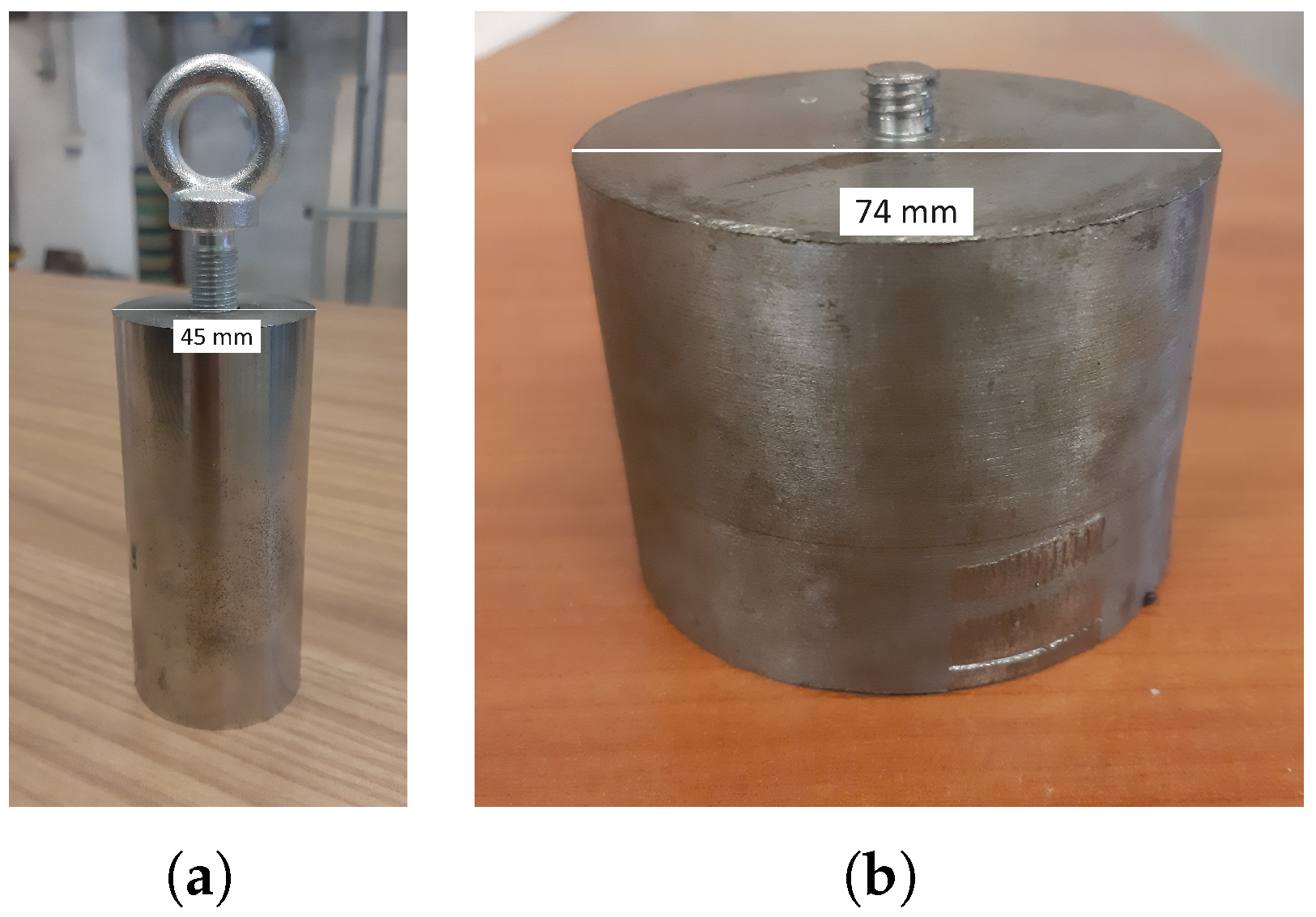
Figure 7.
Impactors: 1.205 kg cylinder (a), cylindrical anvil of the 5.6 kg impactor (b).
Figure 7.
Impactors: 1.205 kg cylinder (a), cylindrical anvil of the 5.6 kg impactor (b).
Figure 8.
Numerical impact analyses: on the top, the meshed geometries prior to compression, on the bottom, the same geometries during compression and shortly before densification, with related contact issues visible in the beam-based models. (a) Sinusoidal lattice: beam (left) and solid meshes (right). (b) Planar anti-chiral lattice: beam (left) and solid meshes (right).
Figure 9.
Low-speed penetration models, top view: the whole geometry (blue) and its symmetric portion (red).
Figure 9.
Low-speed penetration models, top view: the whole geometry (blue) and its symmetric portion (red).
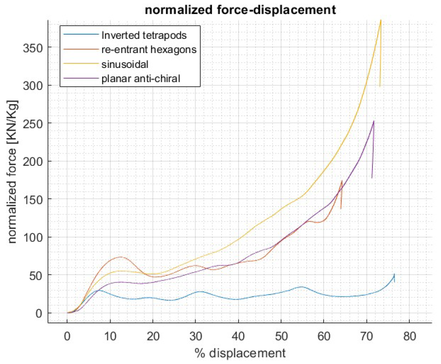
Figure 10.
Quasi-static test results.
Figure 10.
Quasi-static test results.
Figure 11.
PAC (left) and SIN (right) quasi-static re-tests and numerical correlation; being the re-tests phase preliminary to the impact testing campaign, more demanding and relevant to the work, few samples were used: two for PAC, and one for the SIN lattice.
Figure 11.
PAC (left) and SIN (right) quasi-static re-tests and numerical correlation; being the re-tests phase preliminary to the impact testing campaign, more demanding and relevant to the work, few samples were used: two for PAC, and one for the SIN lattice.
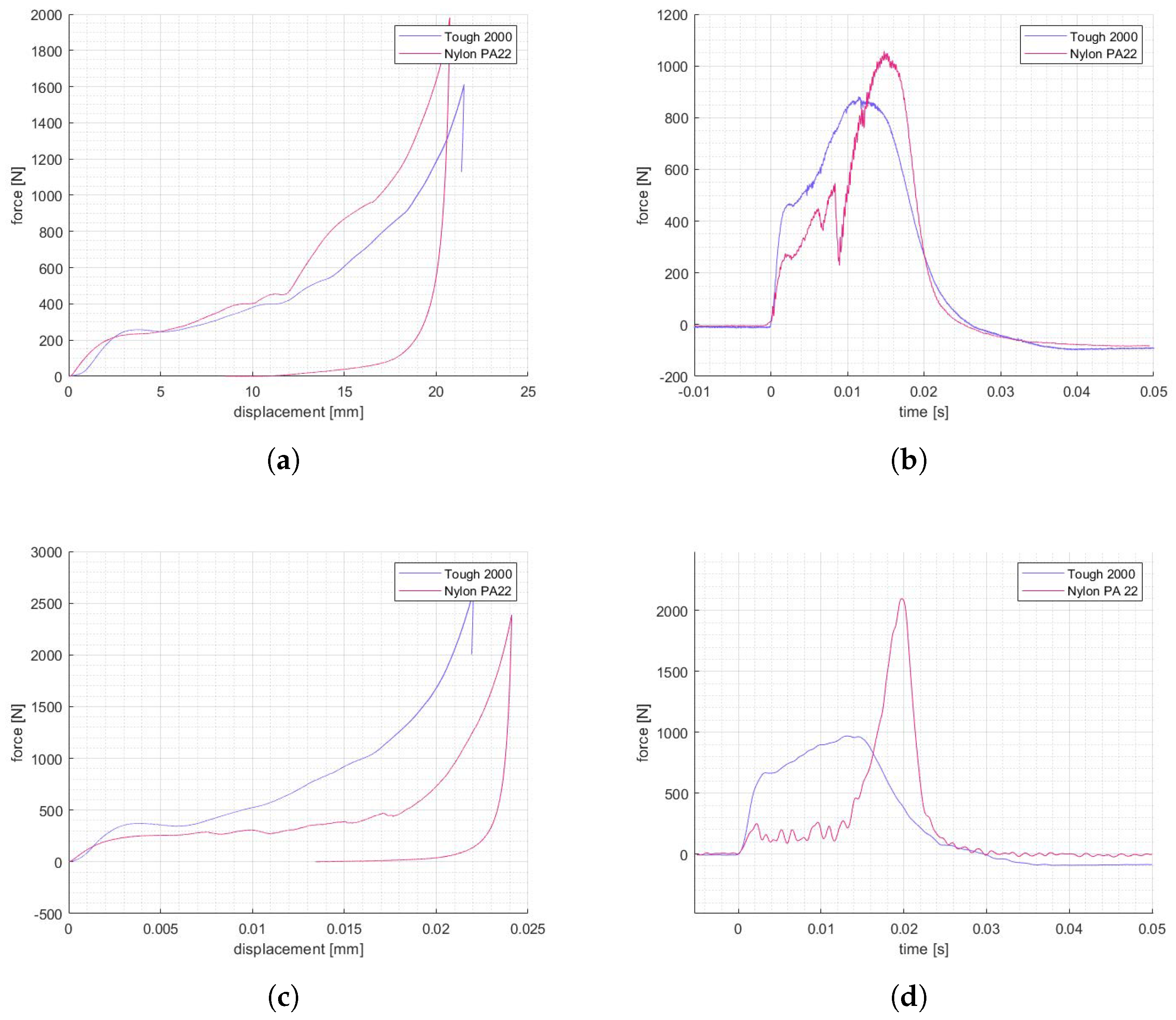
Figure 12.
Static (a) and impact (b) compression of PAC lattices, static (c) and impact (d) compression of SIN lattices.
Figure 12.
Static (a) and impact (b) compression of PAC lattices, static (c) and impact (d) compression of SIN lattices.
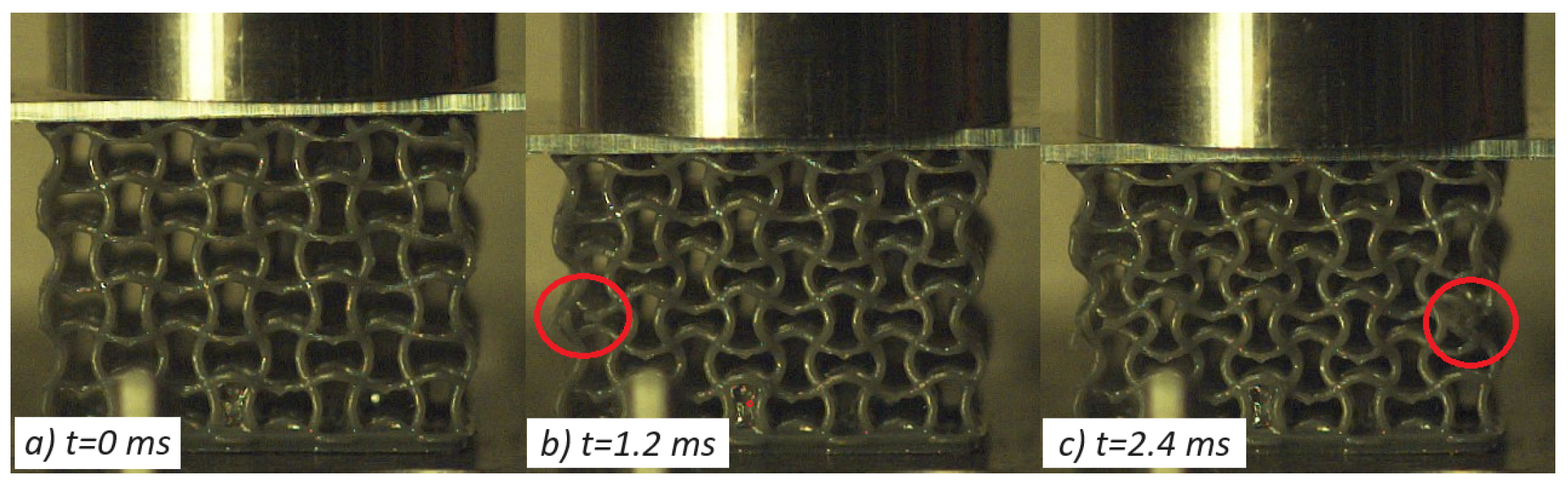
Figure 13.
Impact test of SIN-T2K at 2.3 J with visible auxetic contraction (c); local failures are highlighted in frames (b,c).
Figure 13.
Impact test of SIN-T2K at 2.3 J with visible auxetic contraction (c); local failures are highlighted in frames (b,c).
Figure 14.
Impact test of PAC-T2K at 2.3 J, with visible auxetic contraction (c); no local failures were reported.
Figure 14.
Impact test of PAC-T2K at 2.3 J, with visible auxetic contraction (c); no local failures were reported.
Figure 15.
Repeated impacts results: PAC Tough 2K (a), SIN Tough 2K (b), PAC PA12 (c), SIN PA12 (d).
Figure 15.
Repeated impacts results: PAC Tough 2K (a), SIN Tough 2K (b), PAC PA12 (c), SIN PA12 (d).
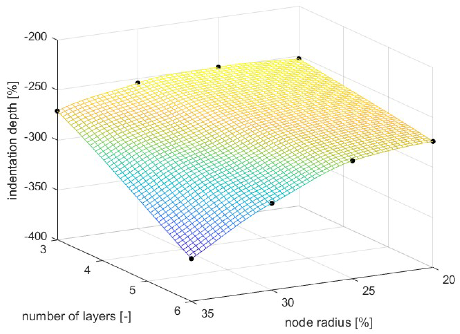
Figure 16.
Penetration analysis of sinusoidal lattice; final results.
Figure 16.
Penetration analysis of sinusoidal lattice; final results.
Figure 17.
Penetration analysis of planar anti-chiral lattice, final results.
Figure 17.
Penetration analysis of planar anti-chiral lattice, final results.
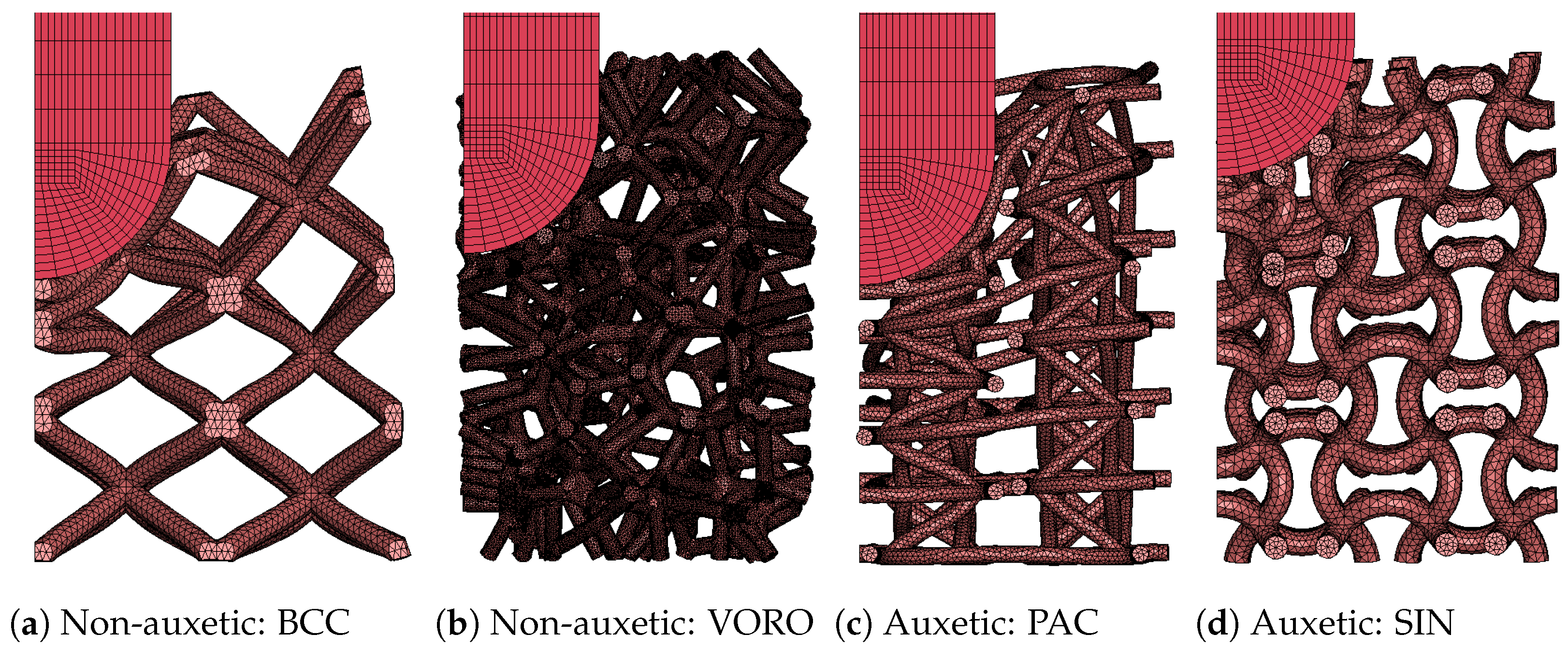
Figure 18.
Penetration analyses at 3 J impact energy. The images capture the maximum vertical displacement of the impactor, showing the penetration resistance of the non-auxetic structures (a,b) with respect to the auxetic ones (c,d).
Figure 18.
Penetration analyses at 3 J impact energy. The images capture the maximum vertical displacement of the impactor, showing the penetration resistance of the non-auxetic structures (a,b) with respect to the auxetic ones (c,d).
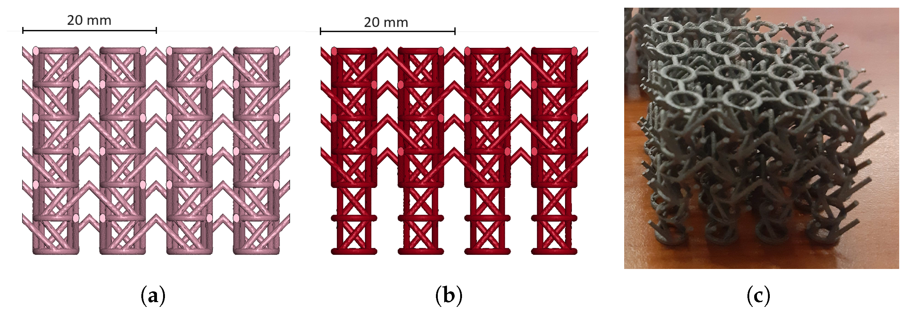
Figure 19.
Modified planar topology, original design (a), defected geometry (b), printed samples (c); as easily seen in (b), the printed samples and numerical models are characterized by missing 45° ligaments on the whole first layer.
Figure 19.
Modified planar topology, original design (a), defected geometry (b), printed samples (c); as easily seen in (b), the printed samples and numerical models are characterized by missing 45° ligaments on the whole first layer.
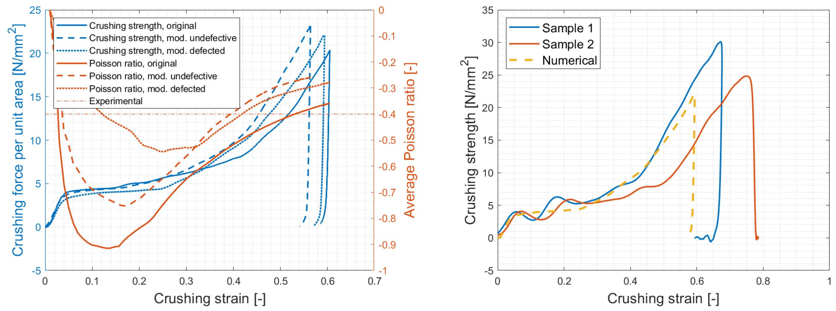
Figure 20.
Numerical analyses of the original, modified defected and undefective geometries (left) and experimental results (right). As mentioned in the text, while the reduction of auxetic effect from original to final geometry is significant (respectively, −0.9, −0.75, −0.54, and −0.4 for original, modified undefected, modified defected and experimental result), notable differences in crushing strength performances were not identified.
Figure 21.
High-speed footage of the modified PAC steel specimen subjected to impact. Prior to densification, occurring at t = 6.6 ms, pronounced transverse contraction can be appreciated at the center of the sample.
Figure 21.
High-speed footage of the modified PAC steel specimen subjected to impact. Prior to densification, occurring at t = 6.6 ms, pronounced transverse contraction can be appreciated at the center of the sample.
Figure 22.
Final numerical results of the modified planar topology: crushing strength (a) and Poisson ratio (b).
Figure 22.
Final numerical results of the modified planar topology: crushing strength (a) and Poisson ratio (b).
Figure 23.
Comparison between auxetic lattices examined (sinusoidal and planar anti-chiral) and a non-auxetic honeycomb.
Figure 23.
Comparison between auxetic lattices examined (sinusoidal and planar anti-chiral) and a non-auxetic honeycomb.
Table 1.
Geometric parameters. h, l, , A, and D, are defined below as a function of the topologies; r represents the strut radius, kept at 0.5 mm for every topology; / is the relative density, expressed as ratio between the density of the cellular solid and the one of the related base material.
Table 1.
Geometric parameters. h, l, , A, and D, are defined below as a function of the topologies; r represents the strut radius, kept at 0.5 mm for every topology; / is the relative density, expressed as ratio between the density of the cellular solid and the one of the related base material.
| Geometry | h (mm) | l (mm) | (deg) | r (mm) | A (mm) | D (mm) | / |
|---|
| IT | 3.5 | 2.64 | 11 | 0.5 | - | - | 0.18 |
| RH | 3.75 | 2.58 | 76 | 0.5 | - | - | 0.28 |
| SIN | - | 5 | - | 0.5 | 1.75 | - | 0.11 |
| PAC | 5 | 10 | 90 | 0.5 | - | 6 | 0.10 |
Table 2.
Geometric parameters for preliminary testing and finalized geometries. Except for the inverted tetrapod geometry, for which the numbers reported in the present table are treated in
Section 2.1.1, all lattices are defined as cuboid-bounded repeatable shapes.
Table 2.
Geometric parameters for preliminary testing and finalized geometries. Except for the inverted tetrapod geometry, for which the numbers reported in the present table are treated in
Section 2.1.1, all lattices are defined as cuboid-bounded repeatable shapes.
| Geometry | Unit Cell
Dimensions (mm) | NCells (-) | Dimensions (mm) |
|---|
| IT | 3.5 × 2.64 | 7 × 9 × 6 | 35 × 40 × 18 |
| REH | 10 × 10 × 10 | 4 × 4 × 4 | 40 × 40 × 40 |
| SIN (preliminary) | 20 × 20 × 10 | 4 × 4 × 2 | 40 × 40 × 30 |
| PAC (preliminary) | 10 × 10 × 10 | 2 × 2 × 2 | 40 × 40 × 20 |
| SIN (finalized) | 20 × 20 × 10 | 4 × 4 × 2 | 40 × 40 × 30 |
| PAC (finalized) | 10 × 10 × 10 | 2 × 2 × 3 | 40 × 40 × 30 |
Table 3.
Materials’ mechanical properties. E is Young’s modulus, is the yield stress, UTS is the ultimate tensile stress, is the failure strain, is the density.
Table 3.
Materials’ mechanical properties. E is Young’s modulus, is the yield stress, UTS is the ultimate tensile stress, is the failure strain, is the density.
| Material | E (MPa) | (MPa) | UTS (MPa) | (%) | |
|---|
| Tough 2000 | 2000 | 38 | 40 | 50 | 1300 |
| PA22 | 1500–1650 | 28 | 48 | 18 | 930 |
| AlSi316L | 180,000 | 530 | 500–600 | 30–40 | 7900 |
Table 4.
Lattice mechanical properties. SEA is the specific energy absorption, E is the elastic modulus, is the collapse stress, is Poisson’s ratio.
Table 4.
Lattice mechanical properties. SEA is the specific energy absorption, E is the elastic modulus, is the collapse stress, is Poisson’s ratio.
| - | SEA (KJ/Kg) | E (MPa) | (MPa) | (-) |
|---|
| Sinusoidal T2K | 2.24 | 3.43 | 0.232 | −0.37 |
| Sinusoidal PA12 | 2.13 | 2.1 | 0.169 | −0.3 |
| Anti-chiral T2K | 1.61 | 2.4 | 0.16 | −0.81 |
| Anti-chiral PA12 | 1.74 | 2.47 | 0.15 | −0.83 |
Table 5.
Multiple impact load peak.
Table 5.
Multiple impact load peak.
| - | Impact 1 (F (N)) | Impact 2 (F (N)) | Impact 3 (F (N)) |
|---|
| Sinusoidal T2K | 983.6 | 1372.2 | 1698.5 |
| Sinusoidal PA12 | 2102.7 | - | - |
| Planar Anti-Chiral T2K | 845.5 | 1031.7 | 1238.2 |
| Planar Anti-Chiral PA12 | 1057.4 | 1796.3 | 2737.6 |
Table 6.
Final penetration results: maximum vertical displacement of the impactor (mm).
Table 6.
Final penetration results: maximum vertical displacement of the impactor (mm).
| Lattice | 30 mm–3 J | 30 mm–7 J | 60 mm–7 J |
|---|
| BCC | 13.6 | 20.3 | 23.2 |
| VORO | 12.3 | 17.1 | 13.2 |
| PAC | 14.1 | 20.5 | 24.1 |
| SIN | 7.9 | 11.5 | 12.8 |

 ,
, 


