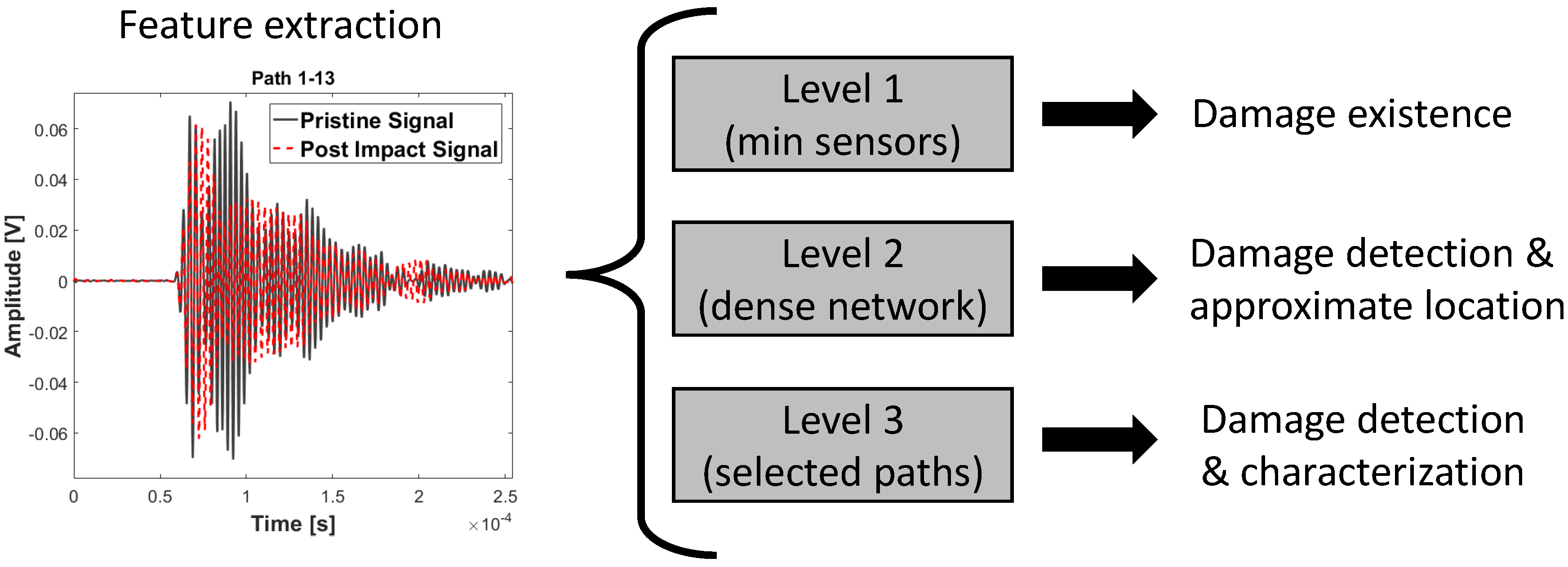
This section will present the developed damage detection and characterisation algorithm as part of a maintenance strategy for a fuselage sub-component (i.e., curved composite stiffened panel) based on a network of distributed PZT transducers and UGW acquisition. The experimental set-up is explained in
Section 2.1. The first step is to evaluate the optimal parameters of the UGW acquisition system such as the actuation frequency, group velocity, attenuation profile based on the pristine state of the structure. After the sub-component is impacted, the post-processing of data are carried out for three different intended functions: Level 1 to determine the existence of damage; Level 2 to determine the existence of damage and its approximate location; and Level 3 to detect and characterize damage (exact location and size). Different methodologies are proposed for each level, as different cost is attributed to each level. The Level 1 diagnosis, as explained in
Section 2.2, is based on the minimum required sensors to detect an existing damage in a large area of the structure; While Level 2, described in
Section 2.3, proposes a detection and localization algorithm and Level 3 in
Section 2.4 results in detection, localization and sizing methodology with minimum required transducers to minimize the cost/time for data acquisition and data handling. Although the proposed approach here is tested and validated for a fuselage panel, it is intended for large structures with multiple areas to be diagnosed, and hence the data acquisition and handling can be of large orders of magnitude. Level 3 diagnostics are referred to as damage characterization i.e., severity and type of damage in addition to its size. However, because the experimental panel was impacted only once to caused BVID, the severity of the damage could not be addressed in this work, and it is intended to be addressed in future works. Before the proposed methodologies are presented, the experimental set up is described in the following section.
2.1. Experimental Set-up
The fuselage panel that has been tested is a composite panel with 790 mm × 1150 mm dimensions and 1978 mm radius of curvature to the outer surface. The skin and omega hat stiffeners were made of T800/M21 uni-directional pre-pregs.
The skin is 1.656 mm thick with (45/−45/90/0/90/0/90/−45/45) layup, whereas the stiffeners are 1.288 mm thick with (45/−45/0/90/0/−45/45) layup. A part of the the panel has been instrumented with 16 DuraAct PZT transducers (PI Ceramics, Karlsruhe, Germany) surface bonded, with cyanoacrylate Loctite 401 adhesive (Henkel, Düsseldorf, Germany), across two bays. The panel was over sensorized to collect as much data as possible and compare the reliability of the detection algorithm for different numbers and locations of transducers. The sensorized area is across two bays to aim for the most challenging case in terms of guided wave damage detection inspecting mid bay and under the stiffeners (see
Figure 2).
The UGWs were recorded using a National Instrument platform with a PXIe single channel arbitrary voltage generator, PXI1 5105 digital oscilloscope and a Pickering 40-726A switching card with maximum output voltage of 12 Volts. To define the optimum parameters of the diagnosis system, the pristine panel has been excited with a five cycle Hanning tone-burst with central frequency range of 50 to 500 kHz in steps of 50 kHz. The signals were then recorded at 60 MS/s sampling rate for 0.001 s. Each transducer path was exited 10 times and signals were recorded, bandpass filtered and averaged to ensure repeatability and to minimize the background noise. The range of signals were then used to find the optimum amplitude, attenuation profile and group velocities of the stiffened panel. The geometry of the sensor network for the sensorized section of the panel is shown in
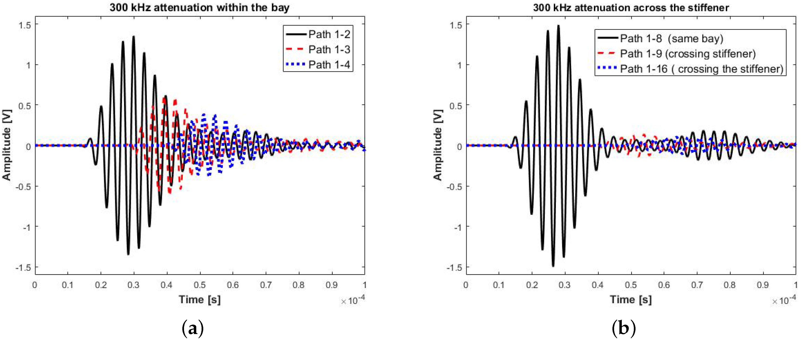
Figure 2b. An example of the attenuation profile for 300 kHz excitation within the bay and across the stiffener is shown in two directions in
Figure 3a,b. It is clearly shown that the attenuation across the stiffener is much more severe than within the bay. The maximum amplitude reduction within the bay is 55%, whereas, across the stiffener, this reduction is as high as 90%. Therefore, it is important to take this into consideration for optimising the number and location of transducers.
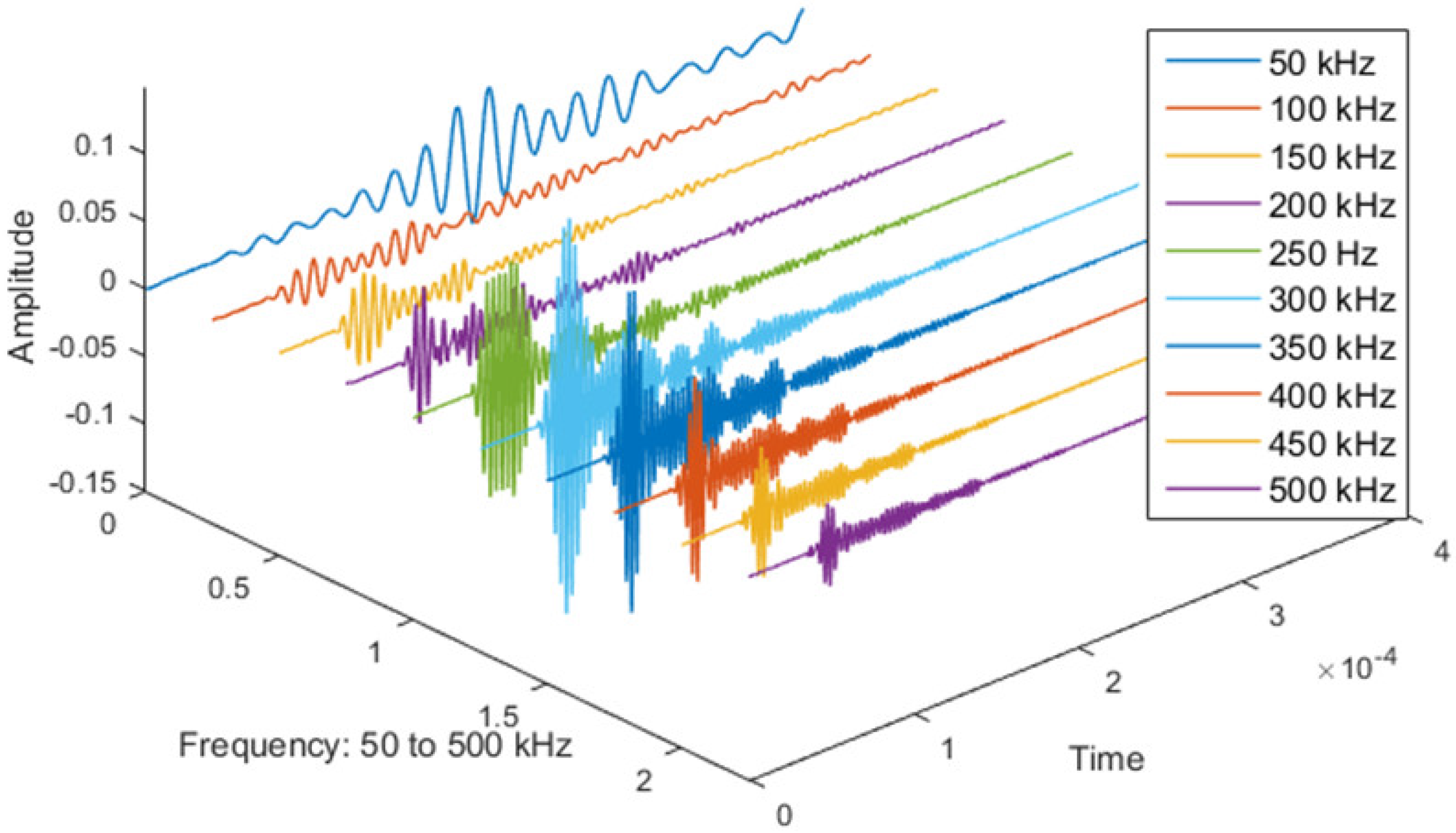
In order to minimize the effect of the attenuation, the frequency with the maximum amplitude response was chosen. The excitation frequency range 50–500 kHz where assessed, and the 300 kHz excitation was chosen as it generated the maximum response in the structure (see
Figure 4).
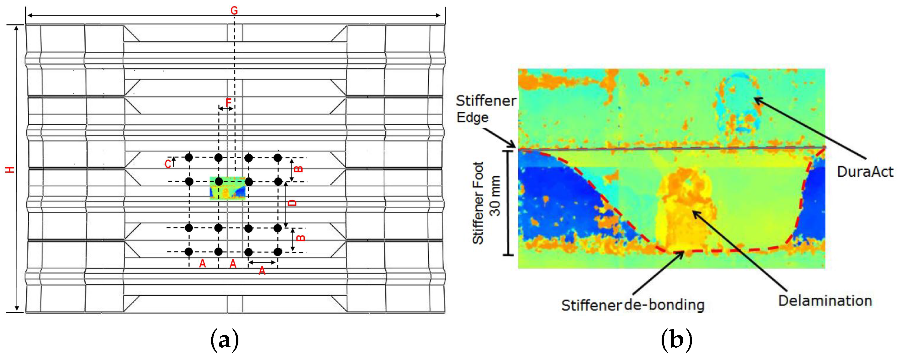
Once all of the pristine data were recorded, the panel was subjected to 50 J impact under the stiffener from the outer skin to induce BVID, i.e., skin/stringer debonding, which represents the most severe case of un-detected damage for a stiffened panel. In addition, detecting skin/stringer debonding is one of the most challenging damage scenarios for the SHM system to detect due to the propagation profile of the guided waves, such as changes in the thickness, additional reflections due to stiffener edges, and attenuation. The location of damage has been indicated by a red X mark in
Figure 2b. An INSTRON CEAST 9350 drop tower with a 20 mm radius hemispherical impactor was used. Both finite element (FE) simulation and experimental results showed that there was a 10% reduction in the compressive strength of the damaged panel [
45]. The C-scan results confirmed a debonded area that was not visible to the naked eye. After the impact, the UGW data were recorded again for damage detection.
2.2. Level 1 Diagnosis: Damage Existence
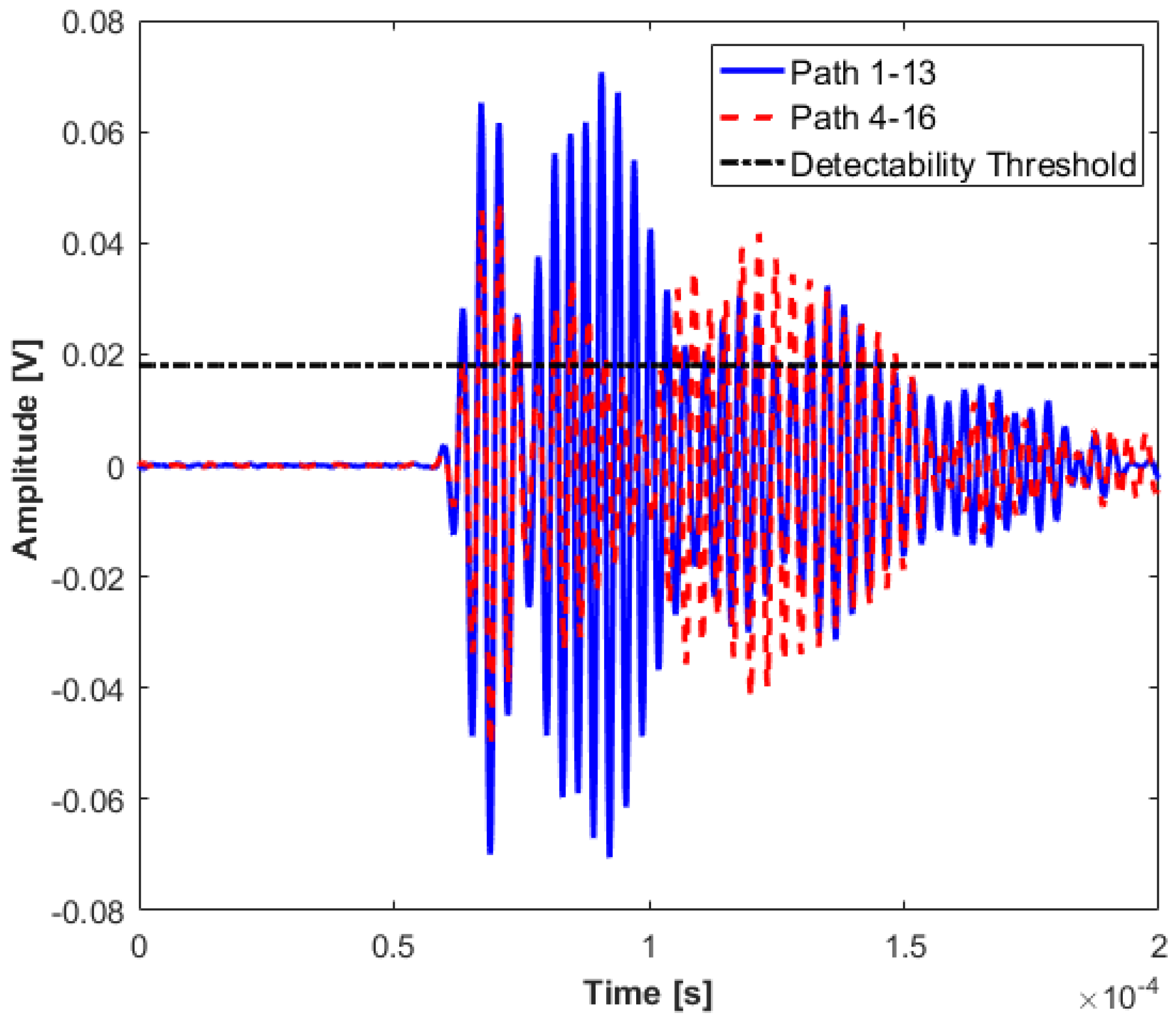
The aim of Level 1 diagnosis is to inform the maintenance engineer of the existence of any damage with minimum cost to the acquisition system. The proposed algorithm for Level 1 aims to cover the maximum area of the structure with the minimum number of transducers. In this case, a transducer network {1 4 13 16} has been chosen for detecting existence of damage. Since the network crosses the stiffener, the first step is to check if the attenuation of the signals is acceptable for detecting any damage inside the sensor network. In theory, reciprocity of the system must hold, which means the signals from path 1-2 must be identical to path 2-1. However, in real structures, there are tolerances with respect to installation of the transducers, which results in small variation in identical paths. These small perturbations have been measured for the total sensor network, and the detectability threshold was set to be 20% above this level to ensure that the attenuation of the signals crossing the stiffener, on its longest paths (i.e., 1-13 and 4-16), does not fall below this limit. As can be seen from
Figure 5, the amplitudes of the signals for the two paths mentioned above are significantly higher than the detectability threshold, and thus the sensor network can be used for Level 1 detection.
Level 1 detection is based on UGWs by comparing the baseline with the current state of the structure, i.e., post impact in this experiment. A damage index (DI) measure is proposed to represent existence of damage where 0 means no damage and 1 indicates damage. The DI proposed for Level 1 is introduced as the maximum energy envelope of the residual signals for each path, where the residual (
) is defined as the difference in the energy envelope between the pristine state (
) and the current state (
) for each path
. The energy envelops difference between the pristine state and the current state is given by:
where
is the Hilbert transform of the residual signal. Then, the DI for each path
ij is defined as the
. Before running the proposed diagnostic algorithm, a threshold value must be defined to indicate damage. To define a damage threshold, usually a large library of baseline measures is required to carry out a statistical analysis to separate the environmental effects from the damage reflected signals. For this experiment, each measurement was repeated 10 times and the reversibility of each path was also used to define a noise threshold at the first stage. The DIs for all the paths of the sensor network {1 4 13 16} are presented in
Figure 6, and the noise threshold is indicated by the red solid line. The values above the noise threshold indicate changes in the signal but not necessarily due to existence of damage. These changes could be attributed to factors such as boundary conditions, loading, temperature, hardware. The second stage is to define a damage threshold to reliably detect the existence of damage. For this reason, the “DI Threshold-Mean” value was identified as the average DI values from all the paths. Any value above this threshold will indicate damage in the close proximity of the path. The impact location is directly over path 1-13 as indicated in
Figure 2b and very close to path 4-16. It is clearly seen that the DI values for these two paths are above the set threshold for damage existence. Another threshold has been defined to indicate a proximal location of damage. This threshold is set as the mean value of all the DIs + the standard deviation and is shown by the dashed green line in
Figure 6. The DI plots clearly indicate damage existence and also approximate location of damage on the path 1-13 as Level 1 detection using only four transducers in the corners to cover a large area within the transducer network.
2.3. Level 2 Diagnosis: Damage Existence and Location
The Level 1 diagnosis resulted in existence of damage and detecting its proximal location, i.e., path 1-13. However, if these results were to be used for a maintenance action, the engineer would then have to monitor a large area of mid-bays, and, under the stiffeners with an NDI technique, localize the damage and take consequent repair actions. If the damage is located in mid-bay, the consequences of not detecting it will not be as severe as debonding of the skin/stringer. Therefore, for some areas, not only the presence of damage is of high importance but to be able to locate it with high precision as well.
There are numerous probability based imaging algorithms that result in damage detection and identification. The methodology which is adopted in this work for localizing and possibly sizing the damage is based on the weighted energy arrival method (WEAM) presented in [
22]. A brief explanation of the method will be given in this section; however, for more detailed overview, please refer to [
22]. The WEAM algorithm is based on a probability damage index for every point in the structure and an imaging algorithm to plot the points with highest probability of damage existence. The damage index at every point in the structure from each transducer path is measured by:
where
is the energy envelope of the residual for the path
ij calculated from Equation (
1), at the location
x,y, and time
t.
is a window function with log-normal distribution centred at the first peak of the residual signal to reduce the effect of boundary reflection and mode superposition.
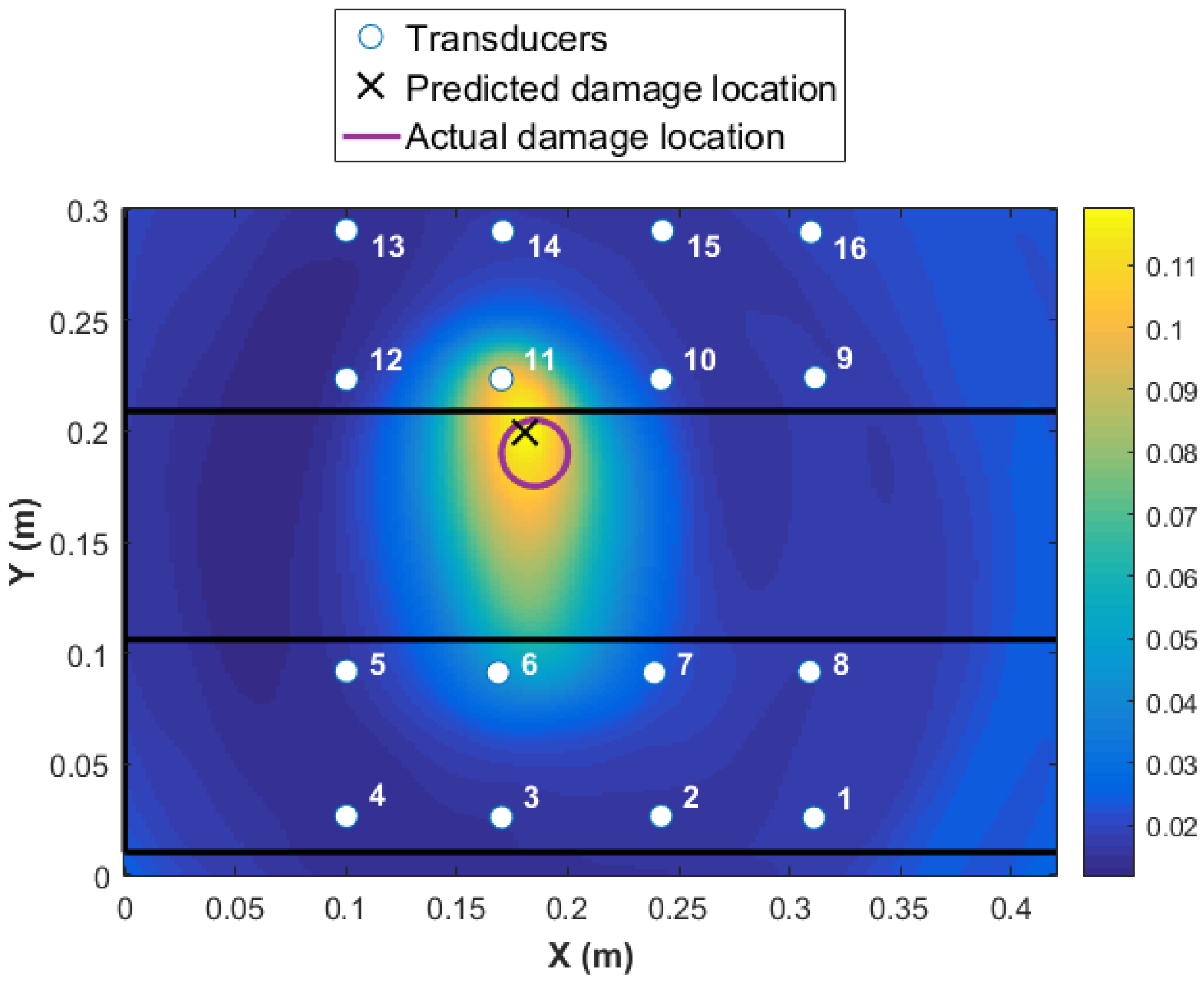
A threshold limit is implemented based on the noise level in the data. At the first step, the data collected from all 16 transducers are used for damage detection and identification as presented in
Figure 7. The colormap in the plot shows the DI values at every point in the structure, with the highest value representing the area with the highest probability of damage existence. The higher the DI value, the more reliable is the diagnosis, i.e., significantly above noise threshold and changes due to operational and environmental conditions. The red circle in
Figure 7 represents the real damage size and area, and the black cross represents the predicted location with the highlighted size. It is shown that the damage is detected with high accuracy. However, to use 16 transducers (240 paths) is expensive in terms of time of the acquisition and data-processing. Each path took about four minutes. In addition, the maximum value of the DI is about 0.12 as presented in
Figure 7. This value is obtained by fusing the residuals from all transducer pairs using an appropriate fusion algorithm, Equation (
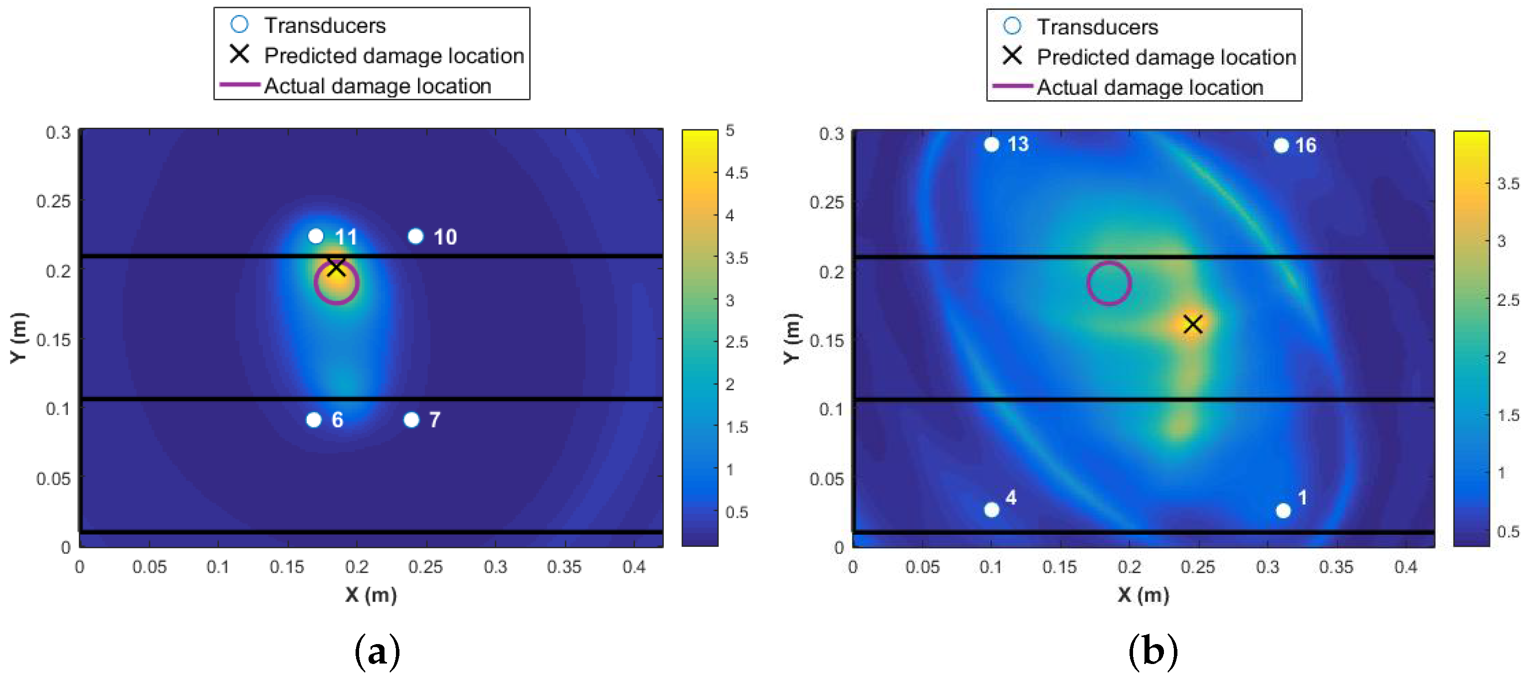
2). Therefore, the contribution of the paths that are far from the damage is negative to the overall detection probability. Ideally, by using the minimum number of paths that are in the proximity of damage, a much higher probability of locating the damage will be reached. For example, if the transducer network {6 7 10 11} is used, the maximum value of DI will increase to five, which is 41 times higher than using 16 transducers. This shows that the reliability of detection is much higher for the four-transducer network because the DI values are far from the noise levels and the damage localization and size is much more accurate (see
Figure 8a). In contrast, if a different combination of four transducers were used with paths that pass close to the damage but further apart from each other, for example, the same sensor network as in Level 1 diagnostics {1 4 13 16}, even though the magnitude of DI remains high for detecting damage reliably, the localization is poor, as presented in
Figure 8b. To demonstrate the sensitivity of the transducer number and location of the damage detection and localization, results from two different networks are presented in
Figure 9.
It is clear from the above results that if the intended function of the SHM system is to locate and characterise the damage in addition to its existence, then a dense network of transducers is required. In contrast, for detecting damage existence, the DI values from four transducers provide values that are significantly above the noise levels. For damage localization to result in accurate damage location, however, not all the transducers are required to be used in the second level diagnosis (see
Figure 8). The question which is now raised is how the user can determine which transducers are to be used in the second- and third-level detection without the prior knowledge of where the impact might have occurred.
2.3.1. A Multi-Level Solution
An important aspect of any proposed diagnostic system is its reliability and probability of detection. This means that the probability of false alarm or misdetection must be minimal. One factor that contributes to false alarm is the failure of the interrogation system, and, in particular, the sensors. PZT transducers are ceramic and thus brittle. Therefore, for real applications, they must be protected—for example, DuraAct transducers (PI Ceramics, Karlsruhe, Germany) have a protection layer. In addition, their bonding to the structure is of high importance, since any deterioration in the bonding quality or connections will result in a change in signal amplitudes and can be identified as false alarms. Therefore, a self-diagnostic scheme must be in place to check the quality of the SHM system (sensors and connections) after installation and prior to its being interrogated for diagnosis to increase the reliability of the decision making process. The self-diagnostic methodology proposed here is based on the EMI measures of the system to detect any faulty sensors [
30].
EMI technique can be used to measure the local dynamical response of a structure at the location of the PZT transducers due to their electro-mechanical coupling. A harmonic voltage is applied to terminals of a PZT transducer and the current propagating through the surface is measured. This is a very attractive method, as each transducer is excited and sensed individually, which simplifies the data acquisition and post-processing. It also reduces the required acquisition time in comparison to UGW acquisitions. When a non-linearity such as damage is present in the vicinity of the transducer, it will change the dynamic response of the structure, and, by comparing its response to a baseline measure, damage can be detected. Damage can either be damage in the transducers (failed sensors, detached sensors) or damage to the structure (delamination, debonding, softening). The electromechanical admittance
Y is defined as the ration between the current
I and the excitation voltage
V. The complex electro-mechanical admittance is expressed as:
where
ω is the excitation frequency and
Q is the electric charge. The impedance is the inverse of the admittance
. The difference in the admittance measured in a healthy structure, and a faulty one is then used to detect damage. This difference in the EMI spectrum measured over a range of frequencies is related to a damage metric value when above a defined threshold.
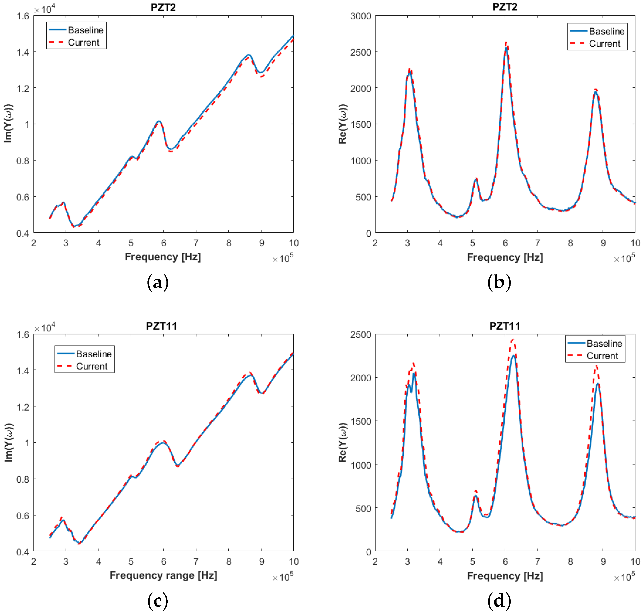
Figure 10 illustrates the changes in the real and imaginary part of admittance measured for a frequency range of 250 to 1 MHz, for two different sensors attached to the composite stiffened panel. PZT2 is located far from the impact damage, whereas PZT11 is very close to the impact site. It can be seen that, while the slope of the imaginary part of the admittance changes slightly (within noise level), the peaks of the real part of admittance changes noticeably for PZT11 when damage is present. This also confirms the findings of other researchers that the slope of the admittance is related to the diagnosis of the sensor alone (i.e., sensor integrity and bonding quality) [
46], and the real part of admittance can be used for detecting damage in the structure in the vicinity of the transducer [
47].
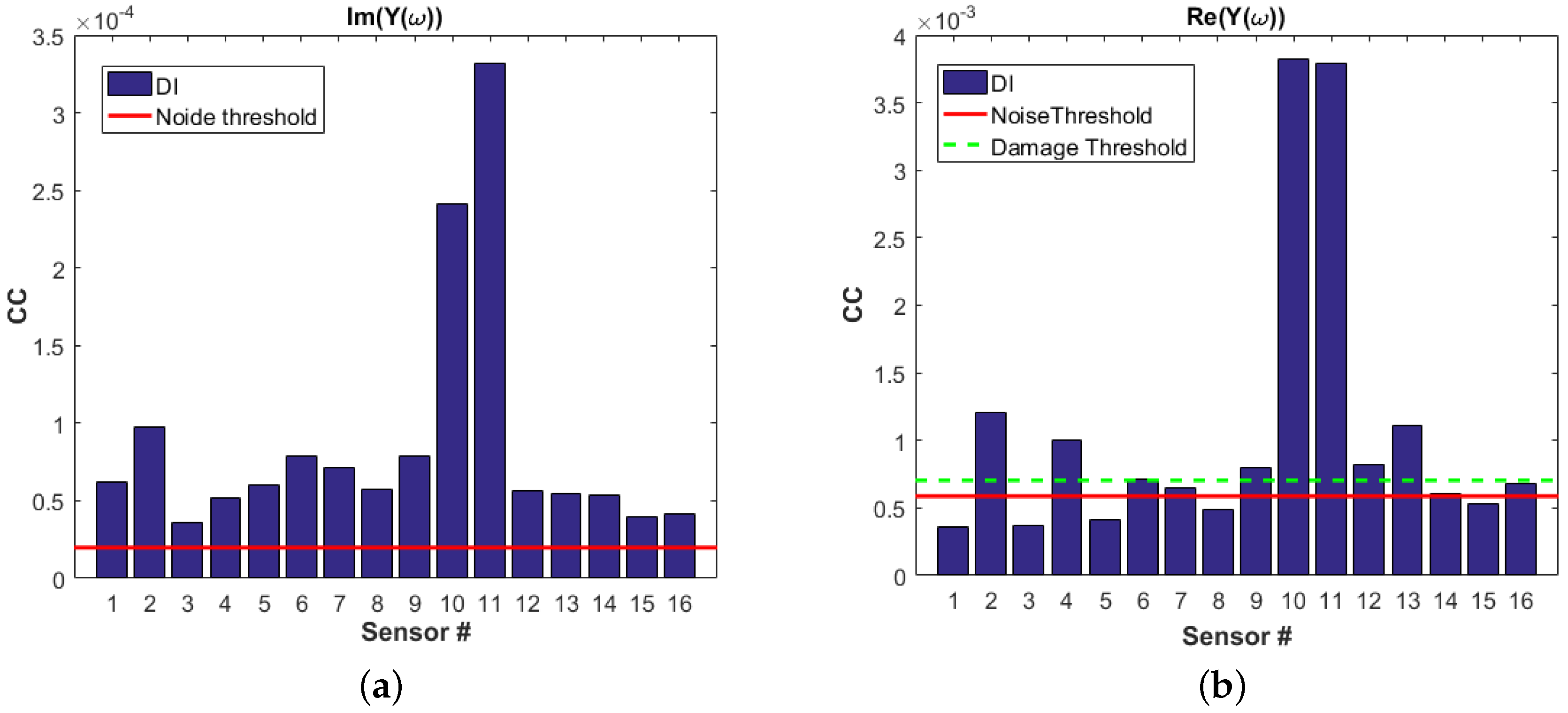
In this work, the damage metric for the EMI approach is defined as the piecewise linear correlation coefficient
between the pristine data and the current data. The noise threshold is measured from the pristine data by averaging the transducer responses measured over several days. The damage threshold then is defined as 20% above the noise threshold.
Figure 11 depicts the DIs in a bar plot for both imaginary and real part of admittance for all transducers and the respective noise thresholds. It is shown that, although both damage metrics show DI values above the noise threshold,
coefficients measured from the real part of admittance are more conclusive with the damage existence in the structure. The DI values for PZT10 and 11 are the highest indicating damage in the vicinity of transducers 10 and 11, which can be validated with the location of the BVID.
2.4. Level 3 Diagnosis: Damage Characterization
By processing the DI values from Level 2 diagnosis, the maintenance engineer can confirm the existence of damage and its proximity to transducers 10 and 11. The exact location, size or type of damage cannot be defined. However, this information can be used in a multi-level diagnostic strategy to reduce the amount of data acquisition and increase the reliability of the decision making. The Level 2 decision making resulted in existence of damage close to transducers 10 and 11. From
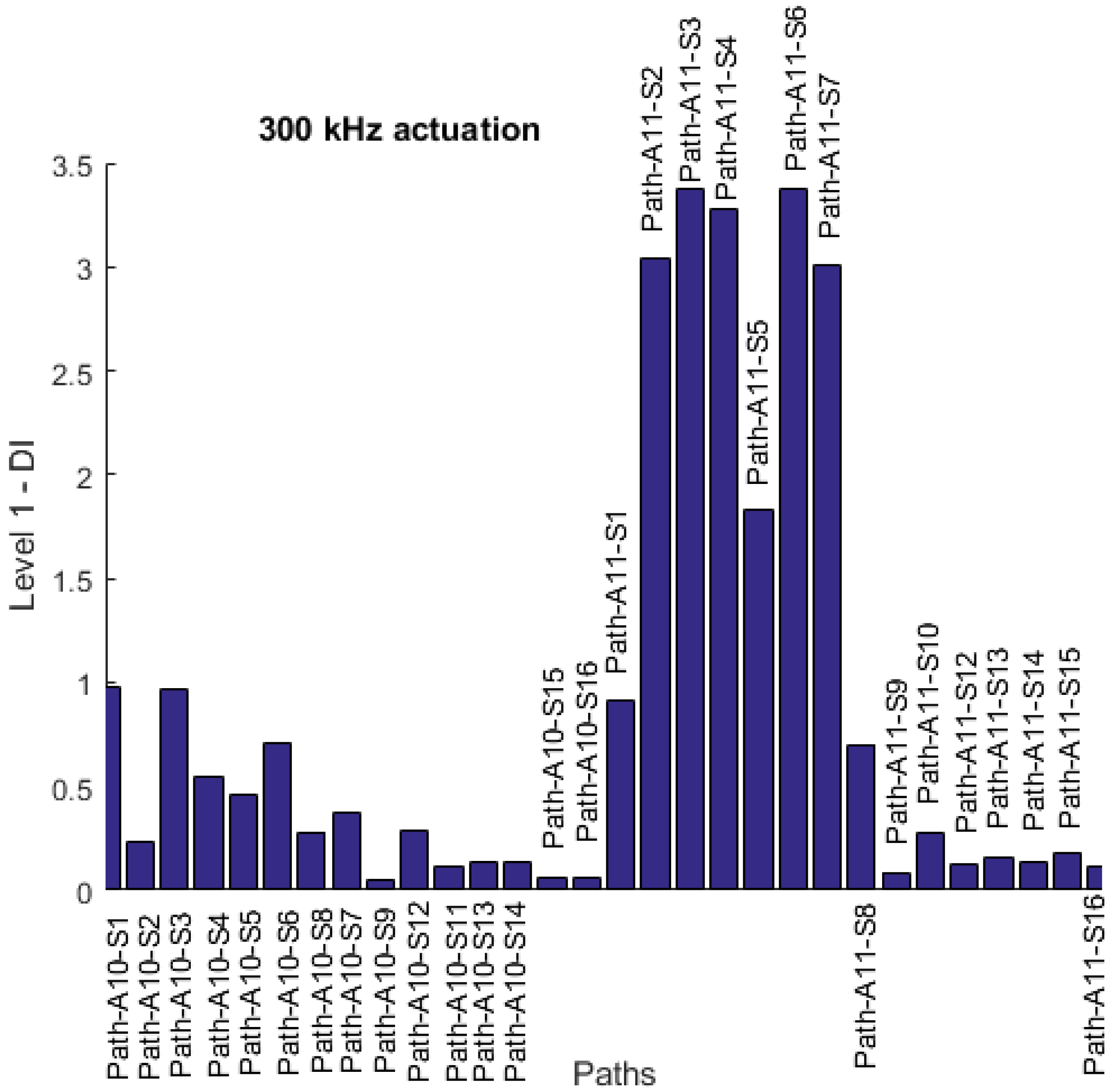
Figure 8, it was concluded that, when applying the WEAM algorithm, to ensure the correct damage characterization, the number of direct paths passing through the damage must be maximized while the paths that are far from damage should be minimized (to increase the reliability). As mentioned before, to cover the whole structure, a dense network of transducers is required. However, for a detailed damage detection and characterization with high reliability, not all of the transducer paths are required to be used. The paths that are far from damage have no positive contributions to the detection algorithm and will have a negative impact on the output of the data fusion. Therefore, Level 3 diagnosis can be built on the decisions from Level 2 to provide a robust damage identification with minimal cost. Level 3 aims to characterize the damage, i.e., its exact location, type and severity. In this work, only the exact location and size has been addressed in Level 3, and the authors are progressing with characterizing the type and severity of damage in future works.
The minimum number of transducers that is required for a delay and sum damage detection algorithm based on triangulation is three. Therefore, from the EMI measures, transducers 10 and 11 are chosen as the two transducers that can be used for a reliable damage localization in Level 3 diagnosis. The reason why these two traducers are chosen is that their DI values are significantly higher than the rest of the transducers and the damage threshold, to ensure reliable selection. There is at least one more transducer required for triangulation. However, the choice of this transducer will have a direct effect on the accuracy of the result. The WEAM will have the best result when the damage is inside the transducer network. The selection criteria proposed in this work is to use the maximum residual path (MRP) to choose a transducer that has the maximum effect of damage presence on its paths. To choose the last transducer required for damage localization, transducers 10 and 11 are used as actuators and using Level 1 damage detection; as described in
Section 2.2, the DI values for all the paths are plotted in
Figure 12. It is observed that maximum residual paths are 11-3 and 11-6. This means that the probability of damage being on these direct paths is the highest. To select between the transducers 3 and 6, the path lengths 11-6 and 11-3 are compared. It can be seen that the path 11-6 is shorter. Therefore, transducer 6 is chosen as the one closer to the damage site. This means that the damage is inside the transducer network {10 11 6}, and the reliability of the damage detection and identification is increased.
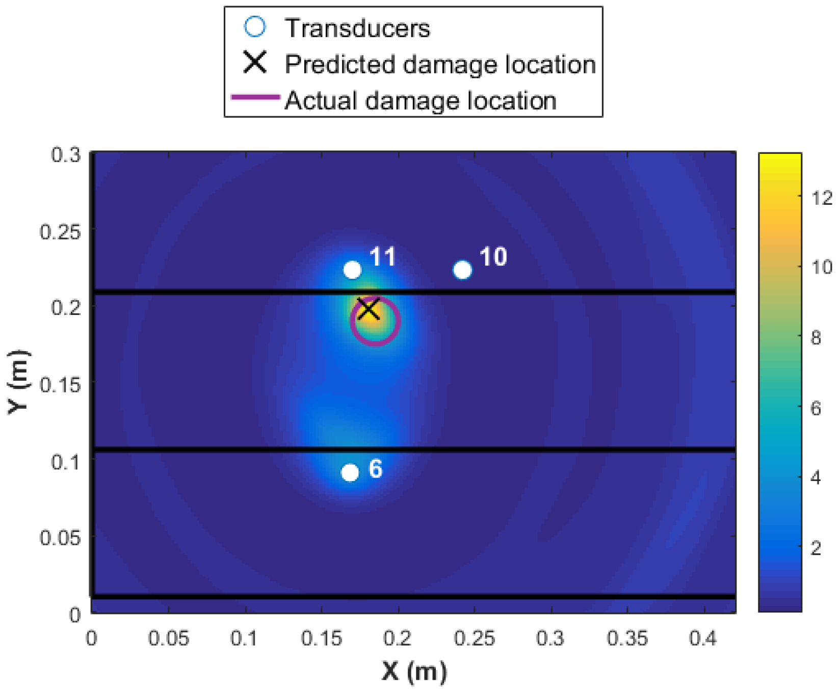
The next step of the multi-level diagnosis is to run the WEAM algorithm using the transducer network {10 11 6}.
The results of Level 3 detection based on the WEAM for the transducer network with MRPs is shown in
Figure 13. It can be seen that not only the accuracy of the detection is increased when using the transducer network based on MRP, but the reliability of detection (increased DI magnitudes) and the accuracy of the damage size has improved significantly. The C-scan results of the stiffened panel post impact is presented in
Figure 14, which validates the damage detection and identification results from the multi-level diagnostic method.
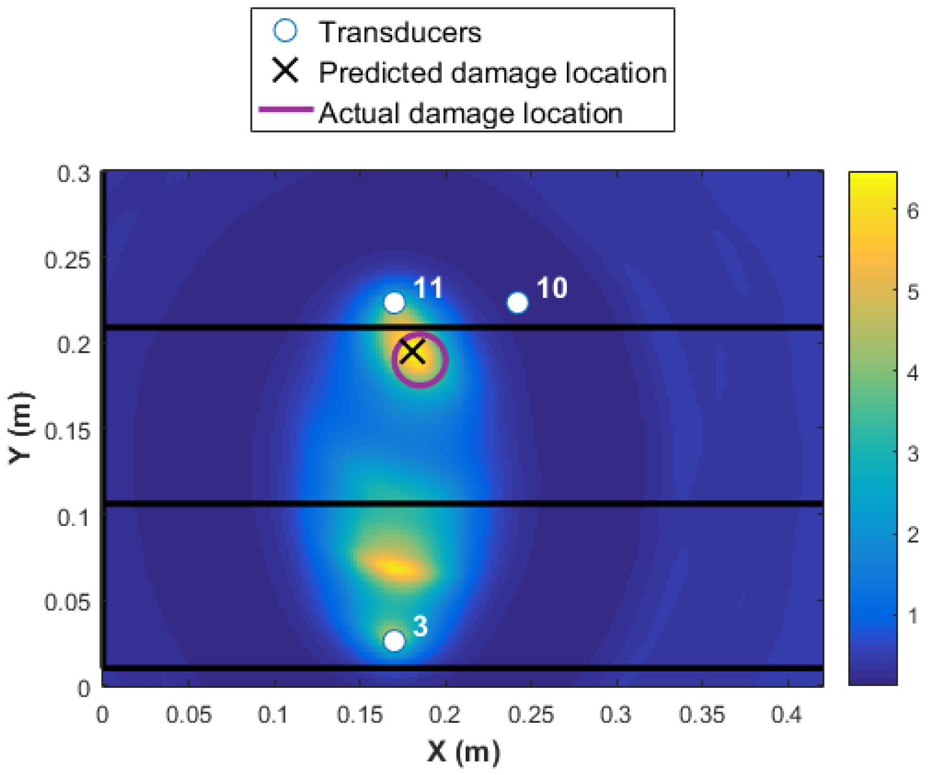
Even if the transducer network {10 11 3} is used for Level 3 damage detection and identification, damage is detected and localized accurately as presented in
Figure 15. However, the reliability is not as high as the MRP transducer network 1 as the maximum amplitude of the DI reduced from 12 to 6, and there is an additional area with a high probability of damage existence close to transducer 3. It is worth highlighting that a network with only three transducers are used in this case, which reduces the signal pre and post-processing significantly (only six transducer paths).


