Allometric Models for Estimation of Forest Biomass in North East India


 , , , , , and
Abstract
:1. Introduction
2. Methods
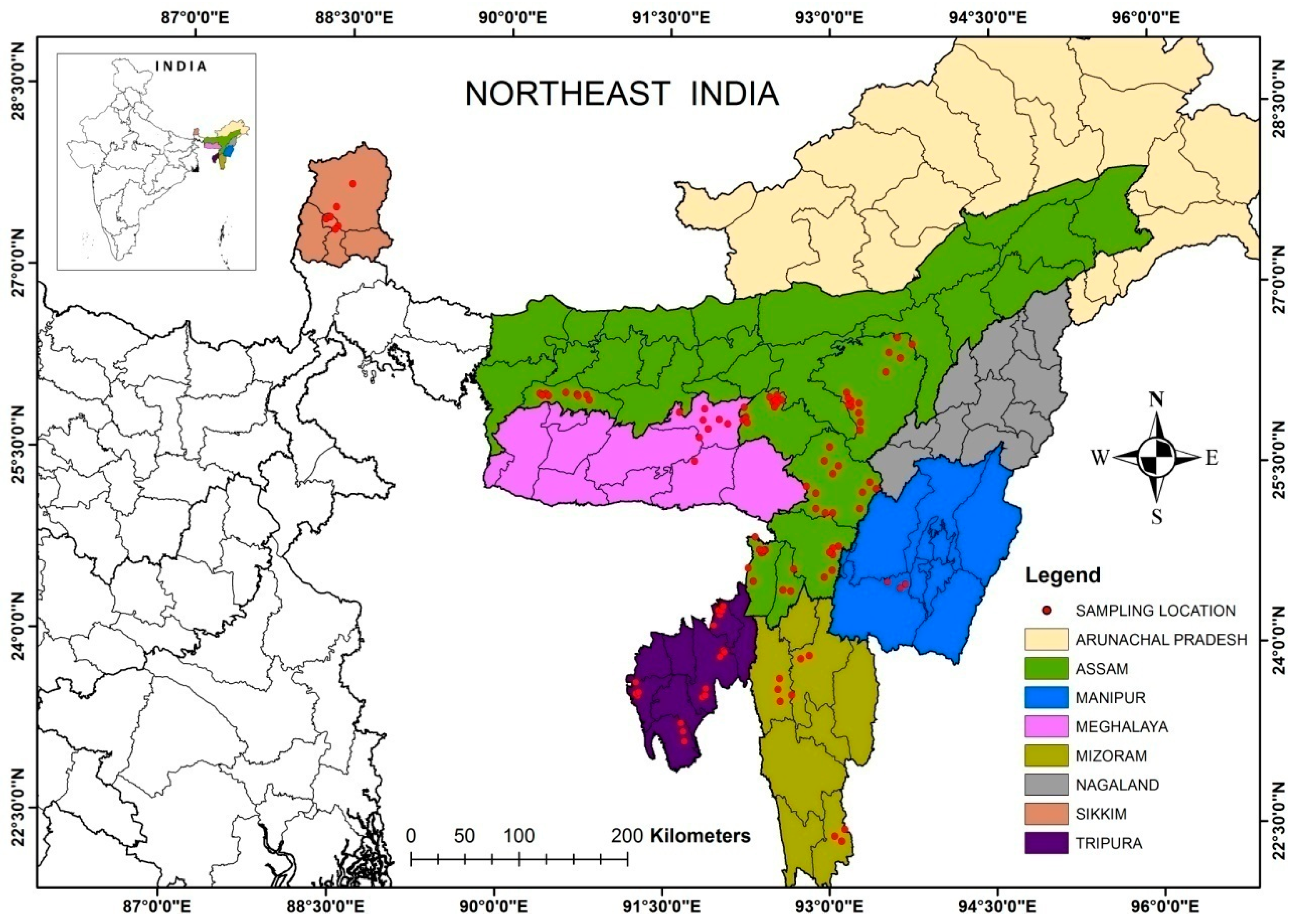
2.1. Descriptions of the Study Region
2.2. Sampling Strategies
2.3. Model Development
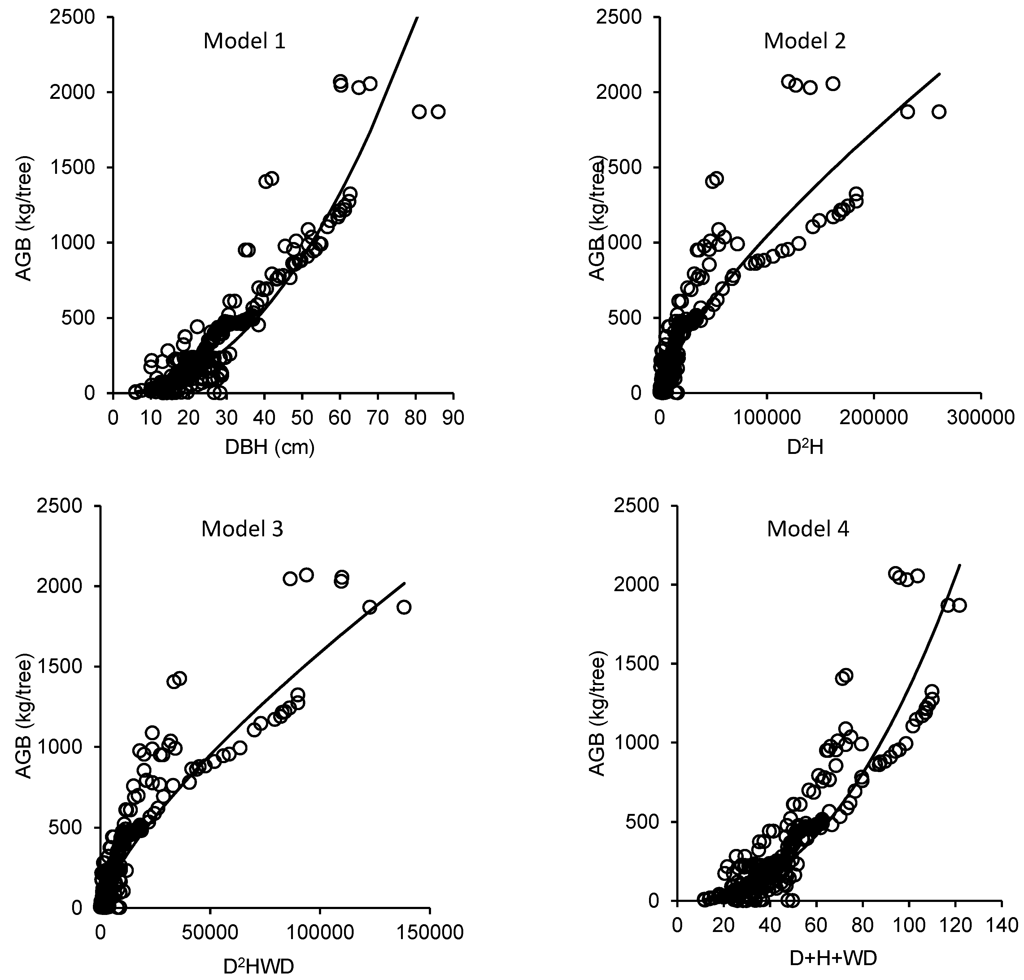
- Model 1:
- ;
- Model 2:
- ;
- Model 3:
- ;
- Model 4:
- Model 1:
- ;
- Model 2:
- ;
- Model 3:
- ;
- Model 4:
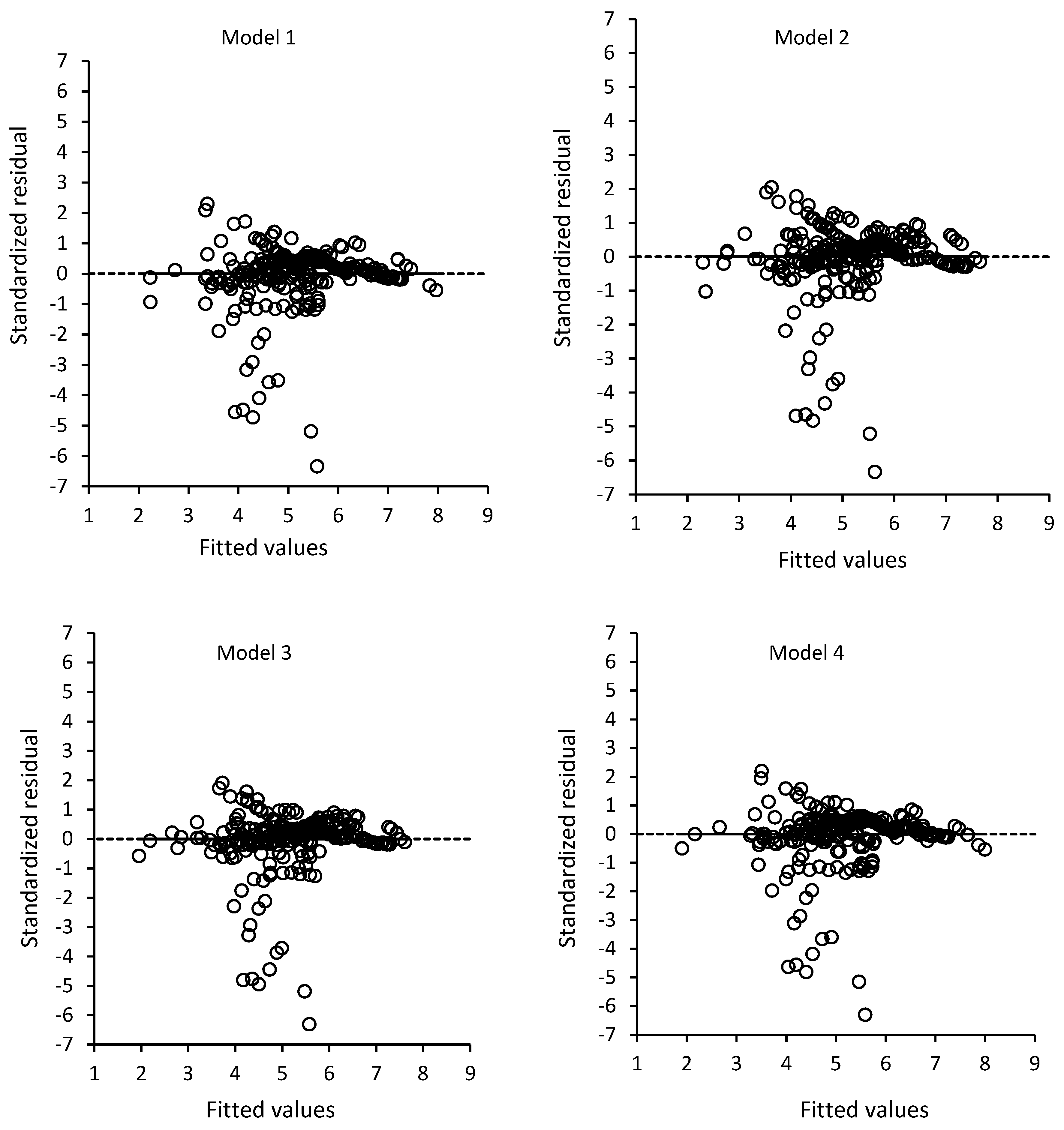
2.4. Model Validation
2.5. Comparison with Generic Models
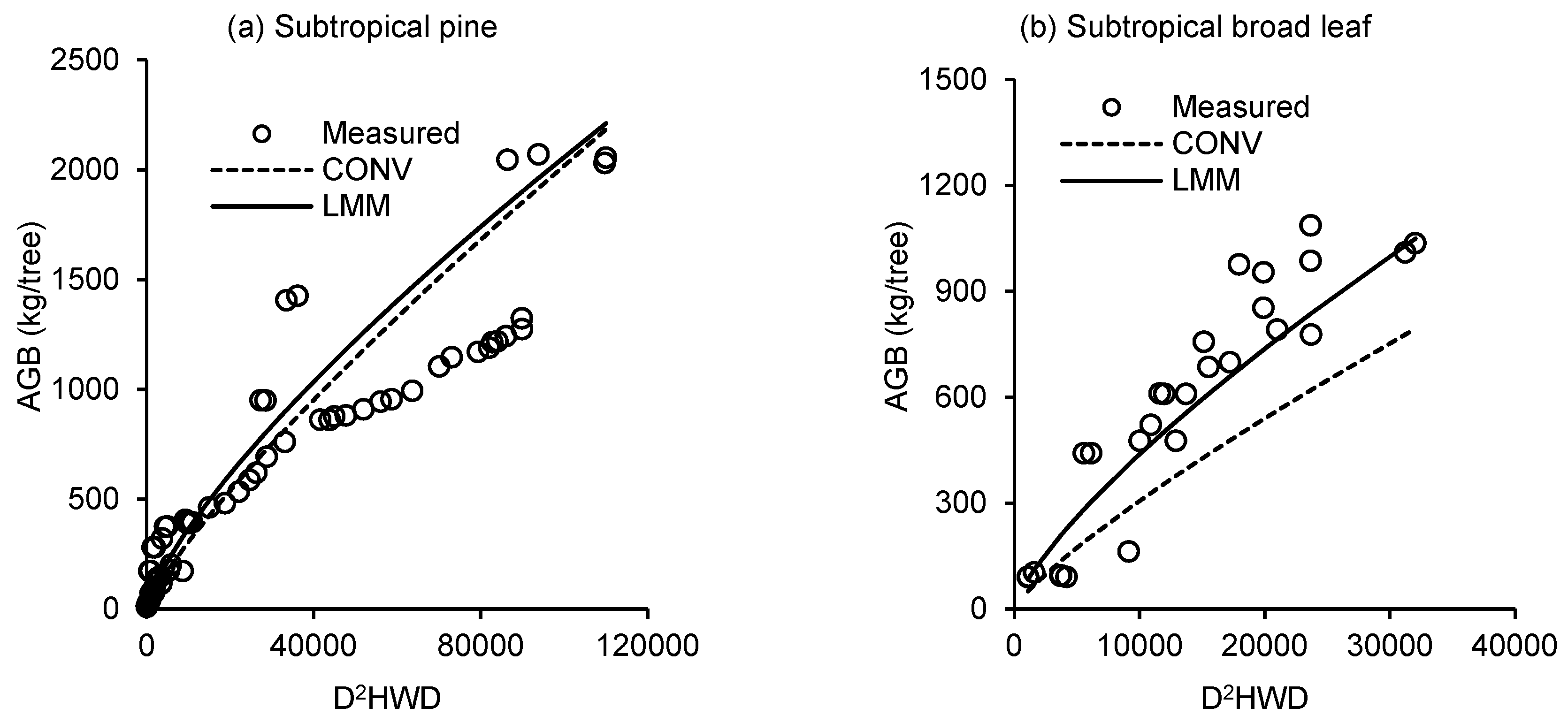
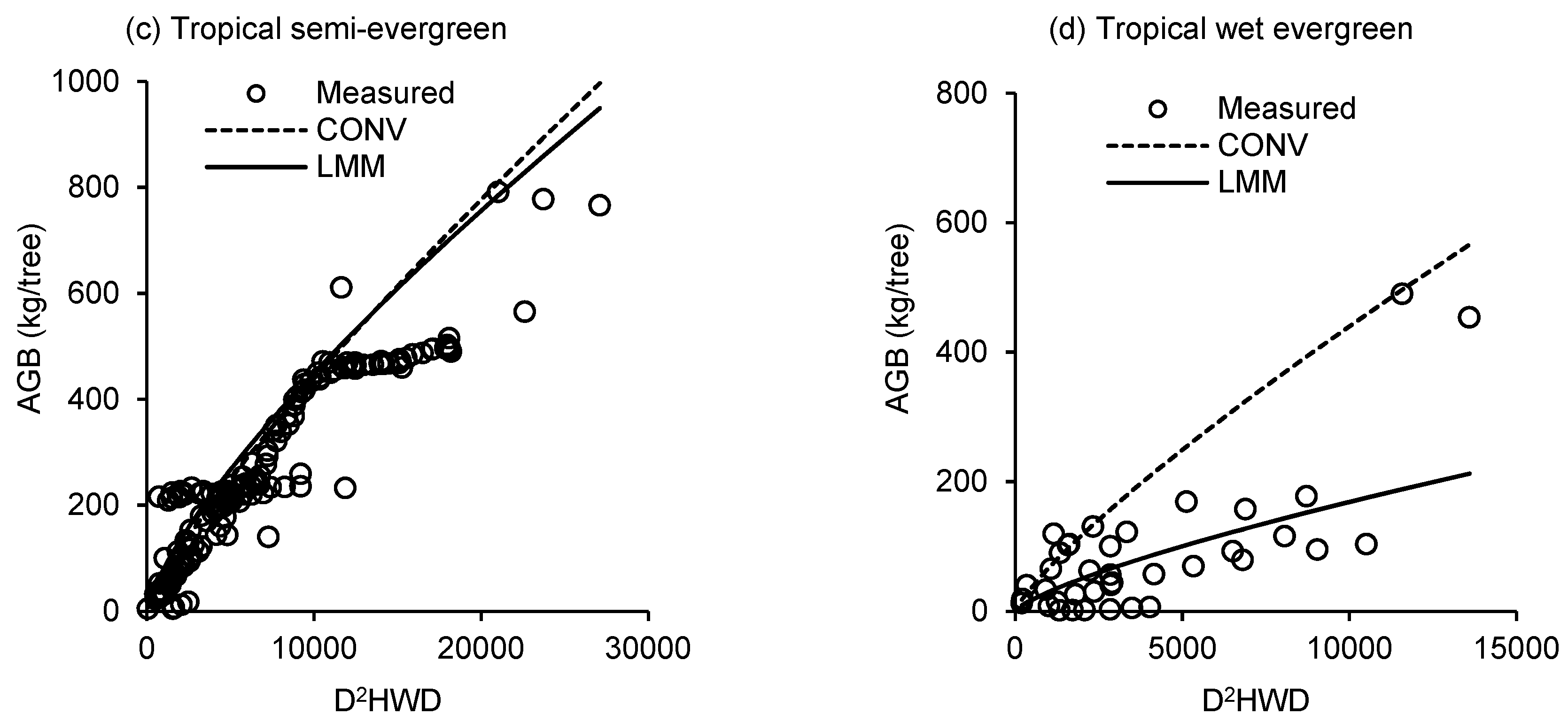
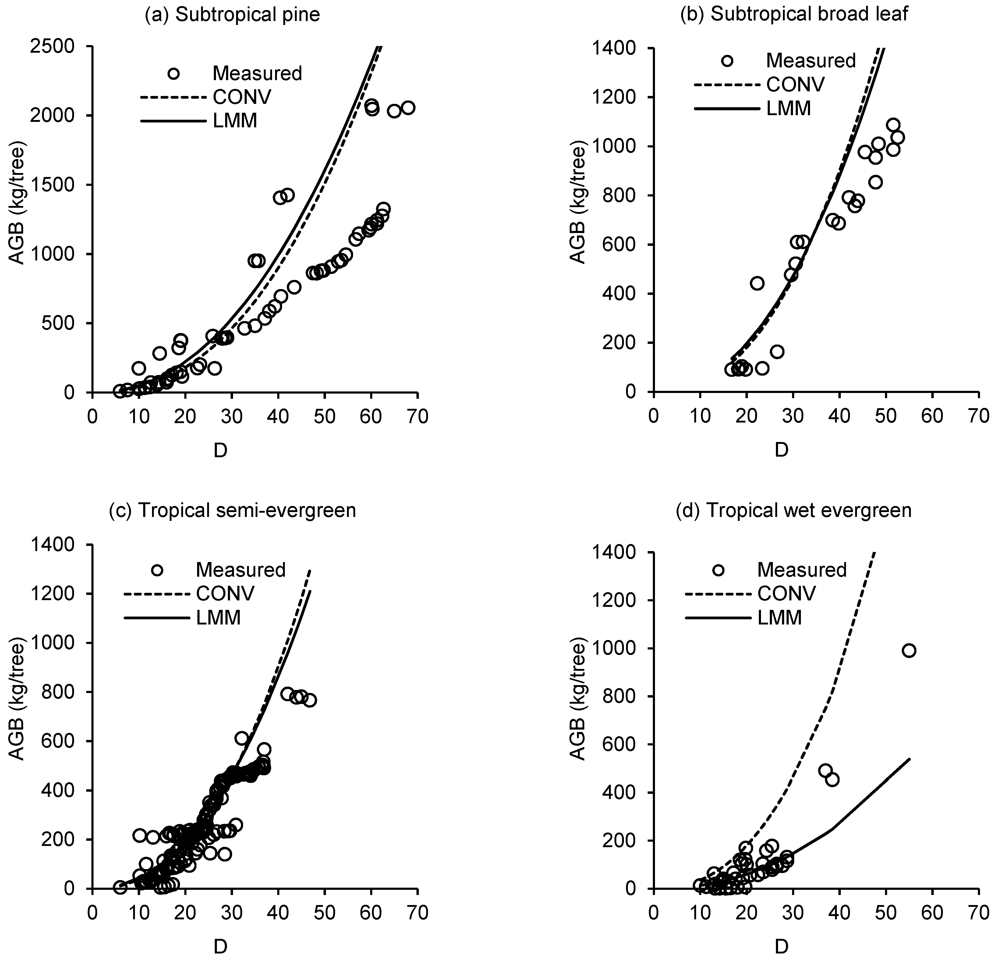
3. Results
4. Discussion
5. Conclusions
Author Contributions
Funding
Acknowledgments
Conflicts of Interest
Availability of Data and Materials
Abbreviations
| Adj R2 | adjusted coefficient of determination |
| AGB | above ground biomass |
| AIC | akaike information criterion |
| BIC | bayesian information criterion |
| BEMs | biomass estimation models |
| CF | correction factor |
| COP | conference of the Parties |
| C | carbon |
| EBLUPs | empirical best linear unbiased predictors |
| CONV | conventional |
| H-D | height-diameter |
| PRESS | prediction residual error sum of square |
| LMM | linear mixed modeling |
| R2 | coefficient of determination |
| REDD | Reducing Emissions from Deforestation and Forest Degradation |
| RMSE | root mean square of error |
| MSE | mean square error |
| NEI | North East India |
Appendix A

| /*Code for fitting Model 1*/ Proc mixed data = Biomass method = REMLcovtest ratio ic; Class Forest; Model lnAGB = lnD/solution outp = check cl; Run; |
| /*Code for fitting Model 2*/ Proc mixed data = Biomass method = REMLcovtest ratio ic; Class Forest; Model lnAGB = lnDDH/solution outp = check cl; Run; |
| /*Code for fitting Model 3*/ Proc mixed data = Biomass method = REMLcovtest ratio ic; Class Forest; Model lnAGB = lnWDDH/solution outp = check cl; Run; |
| /*Code for fitting Model 4*/ Proc mixed data = Biomass method = REMLcovtest ratio ic; Class Forest; Model lnAGB = lnDlnHlnW/solution outp = check cl; Run; |
| /*Code for fitting Model 1*/ Proc mixed data = Biomass method = REMLcovtest ratio ic; Class Forest; Model lnAGB = lnD/solution outp = check cl; Random Forest; ESTIMATE “1” intercept 1| Forest 1; ESTIMATE “2” intercept 1| Forest 0 1; ESTIMATE “3” intercept 1| Forest 0 0 1; ESTIMATE “4” intercept 1| Forest 0 0 0 1; Run; |
| /*Code for fitting Model 2*/ Proc mixed data = Biomass method = REMLcovtest ratio ic; Class Forest; Model lnAGB = lnDDH/solution outp = check cl; Random Forest; ESTIMATE “1” intercept 1| Forest 1; ESTIMATE “2” intercept 1| Forest 0 1; ESTIMATE “3” intercept 1| Forest 0 0 1; ESTIMATE “4” intercept 1| Forest 0 0 0 1; Run; |
| /*Code for fitting Model 3*/ Proc mixed data = Biomass method = REMLcovtest ratio ic; Class Forest; Model lnAGB = lnWDDH/solution outp = check cl; Random Forest; ESTIMATE “1” intercept 1| Forest 1; ESTIMATE “2” intercept 1| Forest 0 1; ESTIMATE “3” intercept 1| Forest 0 0 1; ESTIMATE “4” intercept 1| Forest 0 0 0 1; Run; |
| /*Code for fitting Model 4*/ Proc mixed data = Biomass method = REMLcovtest ratio ic; Class Forest; Model lnAGB = lnDlnHlnW/solution outp = check cl; Random Forest; ESTIMATE “1” intercept 1| Forest 1; ESTIMATE “2” intercept 1| Forest 0 1; ESTIMATE “3” intercept 1| Forest 0 0 1; ESTIMATE “4” intercept 1| Forest 0 0 0 1; Run; |
| Model1<-lm(lnAGB ~ lnD, data = Biomass_data) Model2<-lm(lnAGB ~ lnDDH, data = Biomass_data) Model3<-lm(lnAGB ~ lnWDDH, data = Biomass_data) Model4<-lm(lnAGB ~ lnD + lnH + lnW, data = Biomass_data) |
| The R script for cross validation using 10-fold using the lava packages: cv(list(Model1, Model2, Model3, Model4), k = 10, data = Biomass_data) |
| Various goodness of fit indices were calculated using the following codes using the “forecast” package of R: Model1_results < -t(data.frame(CV(Model1))) Model2_results < -t(data.frame(CV(Model2))) Model3_results < -t(data.frame(CV(Model3))) Model4_results < -t(data.frame(CV(Model4))) Model_results < -rbind(Model1_results, Model2_results, Model3_results, Model4_results) |


References
- Bloom, A.; Exbrayat, J.; van der Velde, I.; Feng, L.; Williams, M. The decadal state of the terrestrial carbon cycle: Global retrievals of terrestrial carbon allocation, pools, and residence times. Proc. Natl. Acad. Sci. USA 2016, 113, 1285–1290. [Google Scholar] [CrossRef]
- Sullivan, M.J.P.; Talbot, J.; Lewis, S.L.; Phillips, O.L.; Qie, L.; Begne, S.K.; Chave, J.; Cuni-Sanchez, A.; Hubau, W.; Lopez-Gonzalez, G.; et al. Diversity and carbon storage across the tropical forest biome. Sci. Rep. 2017, 7, 39102. [Google Scholar] [CrossRef] [Green Version]
- Hosonuma, N.; Herold, M.; De Sy, V.; De Fries, R.S.; Brockhaus, M.; Verchot, L.; Angelsen, A.; Romijn, E. An assessment of deforestation and forest degradation drivers in developing countries. Environ. Res. Lett. 2012, 7, 044009. [Google Scholar] [CrossRef] [Green Version]
- UNFCCC. Modalities for National Forest Monitoring Systems. 2013. Available online: http://unfccc.int/files/meetings/warsaw_nov_2013/decisions/application/pdf/cop19_fms.pdf (accessed on 10 October 2018).
- Harris, N.L.; Brown, S.; Hagen, S.C.; Saatchi, S.S.; Petrova, S.; Salas, W.; Hansen, M.C.; Potapov, P.V.; Lotsch, A. Baseline map of carbon emissions from deforestation in tropical regions. Science 2012, 336, 1573. [Google Scholar] [CrossRef]
- Mitchard, E.T.A.; Saatchi, S.S.; Baccini, A.; Asner, G.P.; Goetz, S.J.; Harris, N.L.; Brown, S. Uncertainty in the spatial distribution of tropical forest biomass: A comparison of pan-tropical maps. Carbon Balance Manag. 2013, 8, 10. [Google Scholar] [CrossRef] [PubMed]
- Woodhouse, I.H.; Mitchard, E.T.A.; Brolly, M.; Maniatis, D.; Ryan, C.M. Radar backscatter is not a ‘direct measure’ of forest biomass. Nat. Clim. Chang. 2012, 2, 556–557. [Google Scholar] [CrossRef]
- Baccini, A.; Goetz, S.J.; Walker, W.S.; Laporte, N.T.; Sun, M.; Sulla-Menashe, D.; Hackler, J.; Beck, P.S.A.; Dubayah, R.; Fried, M.A.; et al. Estimated carbon dioxide emissions from tropical deforestation improved by carbon-density maps. Nat. Clim. Chang. 2012, 2, 182–185. [Google Scholar] [CrossRef]
- Zarin, D.J. Carbon from tropical deforestation. Science 2012, 336, 1518–1519. [Google Scholar] [CrossRef]
- Canadell, J.; Raupach, M.R. Managing forests for climate change mitigation. Science 2008, 320, 1456. [Google Scholar] [CrossRef]
- Pelletier, J.; Ramankutty, N.; Potvin, C. Diagnosing the uncertainty and detectability of emission reduction for REDD+ under current capabilities: An example for Panama. Environ. Res. Lett. 2011, 6, 024005. [Google Scholar] [CrossRef]
- Poulter, B.; Hattermann, F.; Hawkins, E.; Zaehle, S.; Sitch, S.; Restrepo-Coupe, N.; Heyder, U.; Cramer, W. Robust dynamics of Amazon dieback to climate change with perturbed ecosystem model parameters. Glob. Chang. Biol. 2010, 16, 2476–2495. [Google Scholar] [CrossRef]
- Goodman, R.C.; Phillips, O.L.; Baker, T.R. The importance of crown dimensions to improve tropical tree biomass estimates. Ecol. Appl. 2014, 24, 680–698. [Google Scholar] [CrossRef] [Green Version]
- Xiao, C.W.; Ceulemans, R. Allometric relationships for below and aboveground biomass of young Scots pines. Fore. Ecol. Manag. 2004, 203, 177–186. [Google Scholar] [CrossRef]
- Montes, N.; Gauquelin, T.; Badri, W.; Bertaudiere, V.; Zaoui, E.H. A non-destructive method for estimating above-ground forest biomass in threatened woodlands. Fore. Ecol. Manag. 2000, 130, 37–46. [Google Scholar] [CrossRef]
- Chave, J.; Andalo, C.; Brown, S.; Cairns, M.A.; Chambers, J.Q.; Eamus, D.; Fölster, H.; Fromard, F.; Higuchi, N.; Kira, T.; et al. Tree allometry and improved estimation of carbon stocks and balance in tropical forests. Oecologia 2005, 145, 87–99. [Google Scholar] [CrossRef] [PubMed]
- Sileshi, G.W. A critical review of forest biomass estimation models, common mistakes and corrective measures. Fore. Ecol. Manag. 2014, 329, 237–254. [Google Scholar] [CrossRef]
- Vashum, K.T.; Jayakumar, S. Methods to estimate aboveground biomass and carbon stock in natural forests—A review. J. Ecosyst. Ecogr. 2012, 2, 1000116. [Google Scholar] [CrossRef]
- Chave, J.; Réjou-Méchain, M.E.; Búrquez, A.; Chidumayo, E.; Colgan, M.S.; Delitti, W.B.; Duque, A.; Eid, T.; Fearnside, P.M.; Goodman, R.C.; et al. Improved allometric models to estimate the aboveground biomass of tropical trees. Glob. Chang. Biol. 2014, 20, 3177–3190. [Google Scholar] [CrossRef]
- Litton, C.M.; Kauffman, J.B. Allometric models for predicting above-ground biome two widespread woody plants in Hawaii. Biotropica 2008, 40, 313–320. [Google Scholar] [CrossRef]
- Vahedi, A.A.; Mataji, A.; Hodjati, S.M.; Djomo, A. Allometric equations for predicting aboveground biomass of beech hornbeam stands in the Hyrcanian forests of Iran. J. For. Sci. 2014, 60, 236–247. [Google Scholar] [CrossRef]
- India State of Forest Report 2017; Ministry of Environment, Forests and Climate Change, Govt of India: New Delhi, India, 2017.
- Baishya, R.; Barik, S.K. Estimation of tree biomass, carbon pool and net primary production of an old-growth Pinus kesiya Royle ex. Gordon forest in north-eastern India. Ann. For. Sci. 2011, 68, 727–736. [Google Scholar] [CrossRef]
- Brahma, B.; Sileshi, G.W.; Nath, A.J.; Das, A.K. Development and evaluation of robust tree biomass equations for rubber tree (Hevea brasiliensis) plantations in India. For. Ecosyst. 2017, 4, 14. [Google Scholar] [CrossRef]
- Nath, S.; Nath, A.J.; Sileshi, G.W.; Das, A.K. Biomass stocks and carbon storage in Barringtonia acutangula floodplain forests in North East India. Biomass Bioenergy 2017, 98, 37–42. [Google Scholar] [CrossRef]
- Baishya, R.; Barik, S.K.; Upadhaya, K. Distribution pattern of aboveground biomass in natural and plantation forests of humid tropics in northeast India. Trop. Ecol. 2009, 50, 295–304. [Google Scholar]
- Borah, N.; Nath, A.J.; Das, A.K. Aboveground biomass and carbon stocks of tree species in tropical forests of Cachar district, Assam North East India. Int. J. Ecol. Environ. Sci. 2013, 39, 97–106. [Google Scholar]
- Borah, M.; Das, D.; Kalita, J.; Prasanna, H.; Borua, D.; Phukan, B.; Neog, B. Tree species composition, biomass and carbon stocks in two tropical forest of Assam. Biomass Bioenergy 2015, 78, 25–35. [Google Scholar] [CrossRef]
- Waikhom, A.C.; Nath, A.J.; Yadava, P.S. Aboveground biomass and carbon stock in the largest sacred grove of Manipur, North East India. J. For. Res. 2018, 29, 425–428. [Google Scholar] [CrossRef]
- Brown, S.; Gillespie, A.J.R.; Lugo, A.E. Biomass estimation methods for tropical forests with application to forestry inventory data. For Sci. 1989, 35, 881–902. [Google Scholar]
- Chambers, J.Q.; Santos, J.D.; Ribeiro, R.J.; Higuchi, N. Tree damage, allometric relationships, and above-ground net primary production in central Amazon forest. Fore. Ecol. Manag. 2001, 152, 73–84. [Google Scholar] [CrossRef] [Green Version]
- Roy, P.S.; Kushwaha, S.P.S.; Murthy, M.S.R.; Roy, A.; Kushwaha, D.; Reddy, C.S.; Behera, M.D.; Mathur, V.B.; Padalia, H.; Saran, S. Biodiversity Characterisation at Landscape Level: National Assessment; Indian Institute of Remote Sensing: Dehradun, India, 2012. [Google Scholar]
- Mittermeier, R.A.; Robles-Gil, P.; Hoffmann, M.; Pilgrim, J.; Brooks, T.; Mittermeier, C.G.; Lamoreux, J.; Da Fonseca, G.A.B. Hotspots Revisited: Earth’s Biologically Richest and Most Endangered Terrestrial Ecoregions; CEMEX: Mexico City, Mexico, 2004. [Google Scholar]
- Champion, H.G.; Seth, S.K. A Revised Survey of the Forest Types of India; Natraj Publishers: Dehradun, India, 1968; p. 404, (Reprinted 2005). [Google Scholar]
- Poffenberger, M.; Barik, S.K.; Choudhury, D.; Darlong, V.; Gupta, V.; Palit, S.; Upadhyay, S. Forest Sector Review of Northeast India; Community Forestry International: Santa Barbara, CA, USA, 2006. [Google Scholar]
- Chen, D.; Huang, X.; Zhang, S.; Sun, X. Biomass modeling of larch (Larix spp.) plantations in China based on the mixed model, dummy variable model, and Bayesian hierarchical model. Forests 2017, 8, 268. [Google Scholar] [CrossRef]
- Jiang, J. Asymptotic properties of the empirical BLUP and BLUE in mixed linear models. Stat. Sin. 1998, 8, 861–885. [Google Scholar]
- Chave, J.; Coomes, D.A.; Jansen, S.; Lewis, S.L.; Swenson, N.G.; Zanne, A.E. Towards a worldwide wood economics spectrum. Ecol. Lett. 2009, 12, 351–366. [Google Scholar] [CrossRef] [Green Version]
- Sileshi, G.W. The fallacy of retification and misinterpretation of the allometry exponent. 2015. Available online: https://www.researchgate.net/profile/Gudeta_Sileshi2/publication/281204953_The_fallacy_of_reification_and_misinterpretation_of_the_allometry_exponent/links/55dc322808aec156b9b008a2/The-fallacy-of-reification-and-misinterpretation-of-the-allometry-exponent.pdf (accessed on 10 October 2018). [CrossRef]
- Nakagawa, S.; Schielzeth, H. A general and simple method for obtaining R2 from generalized linear mixed-effects models. Methods Ecol. Evol. 2013, 4, 133–142. [Google Scholar] [CrossRef]
- Das, K.; Jiang, J.; Rao, J.N.K. Mean squared error of empirical predictor. Ann. Stat. 2004, 32, 818–840. [Google Scholar] [Green Version]
- Stegen, J.C.; Swenson, N.G.; Valencia, R.; Enquist, B.J.; Thompson, J. Above-ground forest biomass is not consistently related to wood density in tropical forests. Glob. Ecol. Biogeogr. 2009, 18, 617–625. [Google Scholar] [CrossRef]
- Molto, Q.; Rossi, V.; Blanc, L. Error propagation in biomass estimation in tropical forests. Methods Ecol. Evol. 2013, 4, 175–183. [Google Scholar] [CrossRef]
- Lima, A.J.N.; Suwa, R.; de Mello Ribeiro, G.H.P.; Kajimoto, T.; dos Santos, J.; da Silva, R.P.; Souza, C.A.S.; Barros, P.C.; Noguchi, H.; Ishizuka, M.; et al. Allometric models for estimating above- and below-ground biomass in Amazonian forests at São Gabriel da Cachoeira in the upper Rio Negro, Brazil. For. Ecol. Manag. 2012, 277, 163–172. [Google Scholar] [CrossRef]
- Paul, K.I.; Radtke, P.J.; Roxburgh, S.H.; Larmour, J.; Waterworth, R.; Butler, D.; Brooksbank, K.; Ximenes, F.; et al. Validation of allometric biomass models: How to have confidence in the application of existing models. For. Ecol. Manag. 2016, 412, 70–79. [Google Scholar] [CrossRef]
- Thaler, R. The Winner’s Curse; Free Press: New York, NY, USA, 1992. [Google Scholar]
- Marra, D.M.; Higuchi, N.; Trumbore, S.E.; Ribeiro, G.H.P.M.; dos Santos, J.; Carneiro, V.M.C.; Lima, A.J.N.; Chambers, J.Q.; Negrón-Juárez, R.I.; Holzwarth, F.; et al. Predicting biomass of hyperdiverse and structurally complex Central Amazon forests—A virtual approach using extensive field data. Biogeosci. Discuss. 2015, 12, 15537–15581. [Google Scholar] [CrossRef]


| Forest Types | Altitudinal Range (Meters) | Species |
|---|---|---|
| Alpine Temperate | >3500 | Data not available for this study |
| Sub-Tropical Pine | 1000–3500 | Pinus kesiya Royle ex Gordon, Pinus roxburghii Sarg. |
| Sub-Tropical Broad Leaved | 900–1900 | Schima wallichii Reinw. ex Blume, Quercus oblongata D. Don, Ficus benghalensis L., Machilus gamblei King ex Hook.f., Mallotus philippensis (Lam.) Muller.-Arg., Myrica sapinda Wall., Terminalia myriocarpa Van Heurck & Mull., Terminalia chebula (Gaertn) Retz, Toona ciliata M.J. Roem, Juglans regia L., Alnus nepalensis D. Don |
| Tropical Wet Evergreen | Up to 900 | Tectona grandis L.f., Macaranga denticulata (Blume) Muller. -Arg., Mesua ferrea L., Dipterocarpus turbinatus C.F.Gaertn |
| Tropical Semi-Evergreen | Up to 600 | Albizia procera (Roxb.) Benth., Syzygium cumini (L.) Skeels, Macaranga peltata (Roxb.) Muller. -Arg., Bauhinia variegata L., Artocarpus chama Buch. –Ham. |
| Model Parameters | Adj | |||||||
|---|---|---|---|---|---|---|---|---|
| Model | ln(a) (SE) † | b (SE) | c (SE) | d (SE) | AIC ‡ | R2 | RMSE | |
| 1 | CONV | −2.12 (0.34) | 2.32 (0.10) | 769 | 0.62 | 0.851 | ||
| LME | −1.73 (0.45) | 2.16 (0.10) | - | 705 | 0.705 | 0.749 | ||
| 2 | CONV | −2.30 (0.35) | 0.82 (0.04) | 771.7 | 0.619 | 0.852 | ||
| LME | −1.64 (0.44) | 0.74 (0.04) | - | 734.5 | 0.675 | 0.785 | ||
| 3 | CONV | −1.83 (0.32) | 0.82 (0.04) | 770.3 | 0.621 | 0.850 | ||
| LME | −1.25 (0.43) | 0.75 (0.04) | - | 725.7 | 0.685 | 0.773 | ||
| 4 | CONV | −2.12 (0.39) | 2.00 (0.16) | 0.43 (0.16) | 0.37 (0.34) | 763.2 | 0.627 | 0.842 |
| LME | −1.21 (0.49) ns | 2.22 (0.16) | −0.08 (0.16) ns | 0.87 (0.30) | 698.8 | 0.710 | 0.740 | |
| Model § | Covariance Parameter | Variance Estimate | Z Value † | p Value ‡ |
|---|---|---|---|---|
| 1 | Forest | 0.38 (0.32) | 1.18 | 0.1187 |
| Residual | 0.56 (0.05) | 12.21 | <0.0001 | |
| 2 | Forest | 0.30 (0.26) | 1.16 | 0.1236 |
| Residual | 0.62 (0.05) | 12.20 | <0.0001 | |
| 3 | Forest | 0.33 (0.28) | 1.17 | 0.1218 |
| Residual | 0.60 (0.05) | 12.20 | <0.0001 | |
| 4 | Forest | 0.45 (0.38) | 1.18 | 0.1182 |
| Residual | 0.55 (0.05) | 12.16 | <0.0001 |
| Model | Adj R2 | RMSE | AICc | BIC |
|---|---|---|---|---|
| 1 | 0.62 | 0.728 | −93.7 | −82.7 |
| 2 | 0.62 | 0.729 | −93.1 | −82.0 |
| 3 | 0.62 | 0.726 | −94.4 | −83.4 |
| 4 | 0.63 | 0.713 | −98.5 | −83.8 |
| Model | R2 | RMSE | Error | MAPE | AICc | b (95% CL) |
|---|---|---|---|---|---|---|
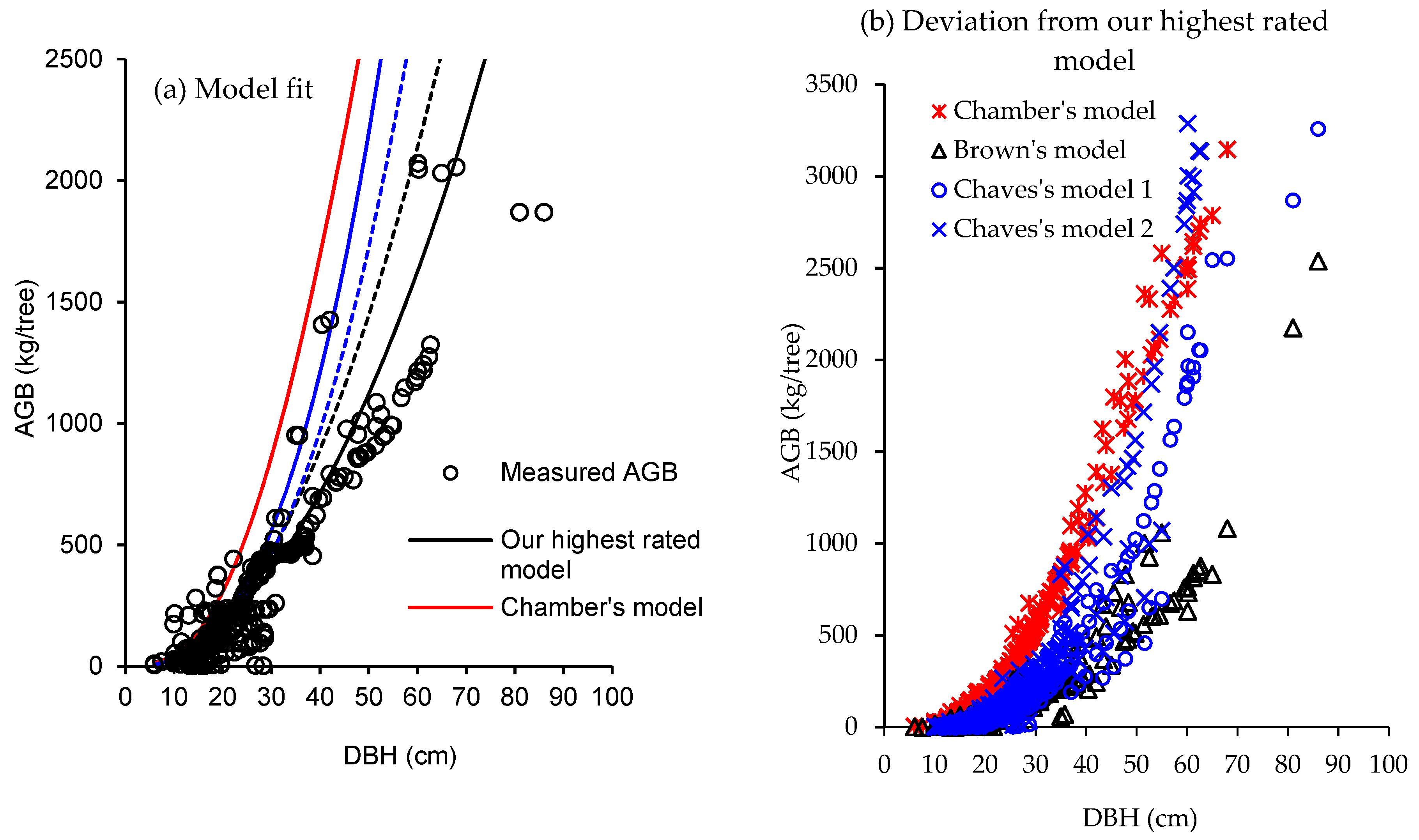
| Our highest rated model | 0.869 | 141 | 197.4 | 235.7 | 3001.8 | 1.06 (1.01–1.11) |
| Chamber’s model | 0.870 | 140 | 591.4 | 595.4 | 2997.9 | 0.33 (0.32–0.35) |
| Brown’s model | 0.848 | 151 | 303.6 | 314.8 | 3045.7 | 0.59 (0.56–0.61) |
| Chave’s model 1 | 0.829 | 161 | 299.6 | 313.2 | 3081.8 | 0.42 (0.40–0.45) |
| Chave’s model 2 | 0.821 | 165 | 372.8 | 382.7 | 3096.5 | 0.32 (0.31–0.34) |
© 2019 by the authors. Licensee MDPI, Basel, Switzerland. This article is an open access article distributed under the terms and conditions of the Creative Commons Attribution (CC BY) license (http://creativecommons.org/licenses/by/4.0/).
Share and Cite
Nath, A.J.; Tiwari, B.K.; Sileshi, G.W.; Sahoo, U.K.; Brahma, B.; Deb, S.; Devi, N.B.; Das, A.K.; Reang, D.; Chaturvedi, S.S.; et al. Allometric Models for Estimation of Forest Biomass in North East India. Forests 2019, 10, 103. https://0-doi-org.brum.beds.ac.uk/10.3390/f10020103
Nath AJ, Tiwari BK, Sileshi GW, Sahoo UK, Brahma B, Deb S, Devi NB, Das AK, Reang D, Chaturvedi SS, et al. Allometric Models for Estimation of Forest Biomass in North East India. Forests. 2019; 10(2):103. https://0-doi-org.brum.beds.ac.uk/10.3390/f10020103
Chicago/Turabian StyleNath, Arun Jyoti, Brajesh Kumar Tiwari, Gudeta W Sileshi, Uttam Kumar Sahoo, Biplab Brahma, Sourabh Deb, Ningthoujam Bijayalaxmi Devi, Ashesh Kumar Das, Demsai Reang, Shiva Shankar Chaturvedi, and et al. 2019. "Allometric Models for Estimation of Forest Biomass in North East India" Forests 10, no. 2: 103. https://0-doi-org.brum.beds.ac.uk/10.3390/f10020103