Identifying European Old-Growth Forests using Remote Sensing: A Study in the Ukrainian Carpathians

1
The Rowans, Thomastown, Huntly AB54 6AJ, UK
2
School of Earth and Environment, University of Leeds, Leeds LS2 9JT, UK
*
Author to whom correspondence should be addressed.
Forests 2019, 10(2), 127; https://0-doi-org.brum.beds.ac.uk/10.3390/f10020127
Submission received: 4 January 2019
/
Revised: 30 January 2019
/
Accepted: 31 January 2019
/
Published: 5 February 2019
(This article belongs to the Special Issue Remote Sensing Technology Applications in Forestry and REDD+)
Abstract
:Old-growth forests are an important, rare and endangered habitat in Europe. The ability to identify old-growth forests through remote sensing would be helpful for both conservation and forest management. We used data on beech, Norway spruce and mountain pine old-growth forests in the Ukrainian Carpathians to test whether Sentinel-2 satellite images could be used to correctly identify these forests. We used summer and autumn 2017 Sentinel-2 satellite images comprising 10 and 20 m resolution bands to create 6 vegetation indices and 9 textural features. We used a Random Forest classification model to discriminate between dominant tree species within old-growth forests and between old-growth and other forest types. Beech and Norway spruce were identified with an overall accuracy of around 90%, with a lower performance for mountain pine (70%) and mixed forest (40%). Old-growth forests were identified with an overall classification accuracy of 85%. Adding textural features, band standard deviations and elevation data improved accuracies by 3.3%, 2.1% and 1.8% respectively, while using combined summer and autumn images increased accuracy by 1.2%. We conclude that Random Forest classification combined with Sentinel-2 images can provide an effective option for identifying old-growth forests in Europe.
1. Introduction
Old-growth forest (OGF), also referred to as primary, virgin or ancient forest, are forests that have developed for a long period of time without significant human intervention and are characterised by the presence of old and large trees, multi-layered vertical structure and abundant standing and lying deadwood in different stages of decay [1,2,3]. OGF are important forest ecosystems, supporting significant biodiversity [4], storing and sequestering large amounts of carbon [5,6,7,8,9] and buffering microclimate [10].
In most European countries, centuries of exploitation have greatly reduced the extent of OGF. There are 1.4 Mha of primary forests remaining in Europe, equivalent to 0.7% of Europe’s forest area [11]. Due to its scarcity and exceptional importance as a habitat for a wide variety of wildlife, conservation of OGF has become an important priority over the past few years. Despite this increased priority, continued loss of OGF from deforestation and conversion to managed plantations is occurring in Europe [12]. While there is no universally agreed definition of OGF, in most cases identification generally involves surveying indicators such as dead wood quantity and quality, forest structure and the degree of anthropogenic influence. This therefore requires time-intensive field surveys. Enabling the identification of such stands by remote sensing would therefore be highly useful. Even establishing the sites of potential OGF stands that could later be verified by field teams could help save time and expense.
While there have been a variety of studies using multispectral remote sensing to identify tree species in Europe [13,14,15,16,17], these are mostly not concerned with OGF. Variation in tree species, height, size and separation as well as the high number of shaded, dead and dying and spectrally unusual trees, mean that tree species in OGF are harder to classify than in other forest types [18]. At the same time, however, this spectral variability can potentially enable the distinction of OGF from younger forest stands.
There have been a number of previous investigations [19,20,21,22,23] into the effect of forest structure on satellite spectra in temperate zones using either Landsat or high resolution satellite imagery, mostly of closed canopy conifer stands (including OGF) in the western USA. Landsat and commercial satellite (10 m resolution) imagery was used to examine how tasselled cap vegetation indices varied with stand characteristics in closed canopy conifer forest in Oregon, USA [20]. Unsupervised classification of Landsat images (tasselled cap vegetation index) was also used in Oregon to map young, mature and old-growth stands [19]. Unsupervised classification of Landsat imagery was used to map mature and old-growth conifer stands in the Pacific Northwest, while Landsat imagery and a spectral mixing model was used to identify stand structural stages in Washington state, USA [23]. There have also been efforts to distinguish mature and old-growth forest using Lidar data and Random Forest classification [24] but Lidar data is usually both expensive and difficult to obtain. Satellite data has been used to identify potential OGF in Romania through manual inspection of images [25]. The recent European Space agency (ESA) Sentinel-2 (S2) mission provides freely available high spatial resolution (10 m) multispectral information and so offers great opportunities for such a forest classification study [26].
The Ukrainian Carpathians contain some of the largest remnants of old-growth fir-beech-spruce-pine forests remaining in Europe. The Carpathian Convention commits Ukraine to the protection of its virgin forests and in May 2017 the Ukrainian president signed an amendment to the Forest Code [27] protecting all OGF sites in Ukraine. An ongoing inventory of OGF in the Ukrainian Carpathians is being carried out by WWF Ukraine and can be viewed at gis-wwf.com.ua/.
In this paper we analyse the spectra of broadleaf, conifer and mixed forests in the Ukrainian Carpathians, using Sentinel-2 imagery and supervised classification to investigate the potential of machine learning to identify OGF, based on the hypothesis that there is a significant difference between the spectra of OGF and other forest types (non-Old-Growth Forest). To the best of our knowledge, this is the first such study employing Sentinel-2 imagery and a decision tree classifier to look at old-growth broadleaf, conifer and mixed broadleaf–conifer woodland in temperate regions. The key objectives of our study are to:
- Use machine learning (Random Forest classification) to identify different tree species in OGF.
- Determine if Random Forest classification can be used to identify and map potential OGF sites by differentiating between OGF and other forest types.
- Determine how combinations of spectral bands, multitemporal imagery and ancillary data affect map accuracy.
2. Material and Methods
2.1. Study Site
We analyse the ability of Sentinel-2 to identify OGF in the eastern Carpathian Mountains of SE Ukraine, a 42% forested region [28] covering about 24,000 km2, ranging from 100–2060 m elevation and characterized in the upper elevations by dense forest stands on steep slopes [29]. Intensive land use and forest management has substantially affected the area’s forests, with much of the lowlands being converted to agriculture. While over the past century forest cover has expanded in the region [30,31], forests are still subject to extensive logging, both legal and illegal [32,33,34] and there are large areas of intensively managed spruce plantations [35]. Nevertheless, the region still contains some of the largest areas of OGF remaining in Europe.
Species composition in OGF in our study site is dominated by beech (Fagus sylvatica L) (33% of area), Norway spruce (Picea Abies (L.) Karst.) (43% of area) and mountain pine (Pinus mugo Turra) (9% of area), with smaller areas of silver fir (Abies alba Mill.) and sessile oak (Quercus petraea (Matt.) Liebl.). Sycamore (Acer psudeoplatanus L), birch (Betula verrucosa Ehrh.), hornbeam (Carpinus betulinus L), rowan (Sorbus aucuparia L), aspen (Populus tremula L), Swiss pine (Pinus cembra L), Scots pine (Pinus sylvestris L), ash (Fraxinus excelsior L), wych elm (Ulmus glabra Huds.), hazel (Corylus avellana L), Norway maple (Acer platanoides L), green alder (Alnus viridis (Chaix.) D.C.) and grey alder (Alnus incana (L.) Moench) occur mixed in small quantities with these species. Tree species show a gradual transition with increased elevation, changing from oak and beech at lower elevations (300–500 m) to beech and Norway spruce dominated (500–1400 m) and to mountain pine and Norway spruce at the highest altitudes (1400–1800 m). Natural alpine meadows cover only the highest of the mountain peaks (>1800 m), though in most places the timberline has been artificially lowered through livestock grazing [36].
Mean annual precipitation varies by altitude from 600 mm in the lowlands to 1600 mm on the mountain peaks [28]. Natural disturbance regimes in the forest are dominated by small-scale loss, largely from low to moderate intensity windthrow damaging single or small groups of trees [37,38,39]. The study region covers three provinces (oblasts): Transcarpathian, Ivano-Frankivska and Chernivetska. Figure 1 (inset map) shows the location of the study area within Ukraine.
2.2. OGF Survey Data
We use data on the spatial distribution of OGF from the ongoing survey (beginning in 2010) of OGF across the Ukrainian Carpathians. This data was provided by WWF Ukraine and covered the survey years 2010–2017 inclusive. This survey includes information on the location and spatial extent of OGF (shapefile polygons of identified OGF stands) as well as detailed information on tree species composition and age. The background to this WWF project and the criteria used for OGF identification can be found here [40]. A map [41] shows the areas surveyed for OGF up to 2017.
The main criteria used in the WWF study for classification of a forest area as OGF are as follows:
- standing and lying dead wood;
- complex structure (high variety of age groups and tree sizes);
- no non-native tree species;
- no visible traces of exploitation—i.e., logging.
While a minimum size criteria (of 20 ha) is given, in practise much smaller areas (down to 0.5 ha) of OGF were also recorded.
A visual inspection of the autumn 2017 Sentinel-2 image showed that since the WWF survey 188 OGF polygons in our study area (mostly Norway spruce forest along the border with Romania) had suffered disturbance through either clear felling, thinning or construction of tracks. These polygons were discarded and not used in our study. Details of the OGF polygons that were used can be seen in Table 1. There were a total of 4037 OGF polygons in our analysis, covering an area of 428 km2. We defined the threshold for mixed forest as 20% and above.
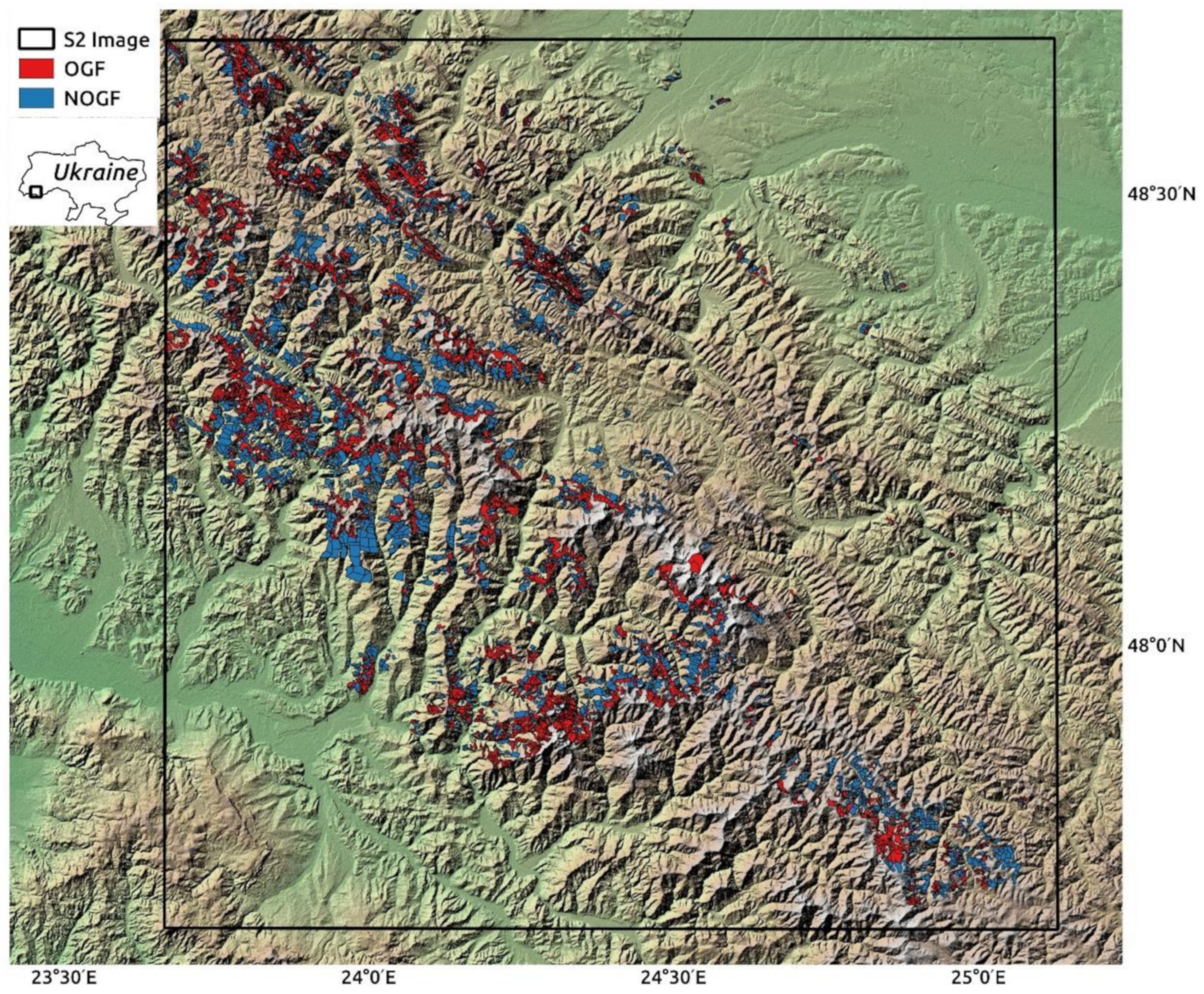
For comparison with OGF polygons, we created 4000 polygons randomly located within a buffer of 2 km of the OGF. This distance was chosen as it enabled the requisite number of appropriately sized NOGF polygons to fit in. To mimic the OGF polygons, polygon sizes were selected from a right-skewed distribution ranging in size from 0.05–200 ha. Polygons which comprised of open areas, non-surveyed areas or young forest were either eliminated or had their boundaries redrawn to exclude these areas. Open areas and young forest was identified either through the publicly available forest cover and forest loss data derived from Landsat timeseries [42] or through visual inspection since open ground and young forest shows up brightly in the images [43]. Since the remaining polygons were forest situated in areas that had been surveyed for OGF yet had not been identified as such, we were confident these polygons consisted of forest that was not OGF (NOGF). These NOGF polygons were then ‘tidied up’ by expansion to remove small gaps between polygons so that they shared a common border. Much of the OGF consisted of high altitude forest stretching up to the treeline. The neighbouring NOGF was therefore typically downhill from the OGF and consequently at a lower elevation and lacking high montane forest. To compensate, we therefore manually created a number of NOGF polygons along the treeline in areas that had been surveyed for OGF. Finally, all these NOGF polygons were classified through visual inspection of Sentinel-2 summer, autumn and winter imagery, as either broadleaved, evergreen or mixed forest. The end result was the creation of 4449 NOGF polygons (described in Table 2), of which a majority lay directly adjacent to the OGF polygons. The median NOGF polygon size was 0.08 km2, compared to 0.07 km2 for the OGF polygons. Figure 1 shows the study region with OGF and NOGF polygons overlaid.
2.3. Sentinel-2 Images
Sentinel-2 (S2) features 13 spectral bands with 10, 20 and 60 m resolution [44]. We used the 10 and 20 m bands in our study (see Table 3). Two S2 images were downloaded (https://scihub.copernicus.eu/) as Level-1C Top-of-Atmosphere reflectance products: one for summer (2 August 2017) and one for autumn (16 October 2017), with codes:
- “S2B_MSIL1C_20170802T092029_N0205_R093_T34UGU_20170802T092027.SAFE” and
- “S2A_MSIL1C_20171016T092031_N0205_R093_T34UGU_20171016T092425.SAFE” respectively.
These particular images were chosen for their low cloud cover (5.2% and 0% respectively). The north-east and south-west corners of these images are 23°43′7.73″ E, 48°43′15.34″ N and 25°7′41.74″ E, 47°41′27.06″ N respectively. These images were then topographically and atmospherically corrected using the Sen2Cor module [45]. The 20 m resolution bands were resampled to 10 m spatial resolution. We investigated using spring or winter images but from December through to April most of the high altitude OGF was completely covered with snow, with the polygons completely white and providing limited useful information.
2.4. Sentinel-2 Image Evaluation
We used an object-based approach (as opposed to a pixel-based classification), where the mean and standard deviation of the pixel spectra and the mean of the associated vegetation indices and textural features within a forest polygon were used for the analysis. A number of studies have argued for the superiority of object-based over pixel-based approaches [15,18,46] and the WWF data included mixed forest polygons which suited an object-based approach. To further understand the distribution of the pixels within the polygons, we also calculated percentile values ranging from 5% to 99% for each polygon. T-tests of the band spectra mean values were calculated to test for significant differences between the OGF and NOGF polygons.
We calculated 6 vegetation indices from the S2 bands: the Normalized Vegetation Difference Index (NDVI) and the Enhanced Vegetation Index (EVI), probably the two most commonly used forest classification indices. Since the more heterogeneous structure of OGF compared to other forest types might help classification, we used two forest structure indices: Advanced Vegetation Index (AVI) and the Shadow Index (SI). A study [20] found the difference between SWIR and NIR bands most useful in distinguishing mature and OGF so we also used Normalised Difference Infrared Index (NDII). Lastly, the Red edge Normalized Difference Vegetation Index (RENDVI) was chosen to exploit information in the red edge bands.
Spectral images vary not only in tone but also in texture (spatial variation). Texture measurements quantitively describe relationships of spectral values with neighbouring pixels, which information has been used previously to improve forest stand classification accuracy [47,48]. The most commonly used textural measure is the Grey Level Co-occurrence Matrix (GLCM) [49], essentially a description of how often different combinations of pixel brightness values (grey levels) occur in an image. A detailed overview of GLCM can be found here [50]. Generally, younger forest have a more uniform and low contrast image due to the trees’ equal height and spatial distribution, whereas the heterogeneity of OGF, with a broader distribution of tree heights and ages, results in more shadows cast by emergent trees. OGF are therefore likely to have differences in texture compared to NOGF areas.
Use of GLCM requires choosing 6 parameters—textural features, pixel displacement and direction, the moving window size, quantisation level and spectral bands – giving rise to thousands of potential combinations. The textural features can be divided into contrast, orderliness and descriptive statistics groups [50]. We chose one textural feature from each of these groups that had been found useful in previous studies [51,52]: contrast, entropy and GLCM mean. Contrast is a weighted measure of the contrast between adjacent pixels—the greater the value the greater the contrast. Entropy corresponds to the orderliness of the image—larger entropy values indicate greater disorder. We calculate these features for a visual, near IR and shortwave IR band (B3, B8 and B12). A study [53] found that for spectrally homogenous classes, smaller window sizes improved classification accuracy. Combined with the coarse resolution of the S2 data, we therefore computed the selected textural variables with a relatively small 5 × 5 pixel window size over all directions, a pixel displacement of 1 and a 32 level quantization using the ESA Sentinel Application Platform (SNAP), available at http://step.esa.int/main/toolboxes/snap.
Mean and standard deviation for each polygon were extracted for each of the 10 bands, as well as the mean of the 6 vegetation indices and the 9 textural measures. Mean elevation and slope was also calculated (using 1 arc second resolution Shuttle Radar Topography Mission (SRTM) data [54]). The number of polygons and area for each forest type are given for OGF and NOGF in Table 1 and Table 2 respectively.
2.5. Random Forest Method
Random Forest (RF) [55] is a non-parametric machine learning algorithm, selected for its high classification accuracy [56,57], ease of use [58,59] and its demonstrated ability in previous remote sensing forest classification studies [15,16,17,60].
The polygons were randomly divided into training and validation sets in a ratio of 75% and 25% respectively. The classification analysis was performed using the scikit-learn Python library [61]. The maximum number of features Random Forest was allowed to try in an individual tree was set as the square root of the total number of features. The number of trees built was set at 500. We found changing these parameters made little difference to model outcome. Feature importance was calculated by mean decrease impurity.
We report user’s accuracy (how reliable is the map, that is, how often forest identified as, say, OGF in our model is actually present on the ground), producer’s accuracy (how well is the situation on the ground mapped, that is, how often OGF on the ground is correctly identified as such by our model) and overall accuracy (how often all our forests were identified correctly). We report accuracy as the average across the relevant polygons.
The Random Forest classification between tree species was carried out using only the 1781 Norway spruce, 1281 beech, 219 mountain pine, 189 beech-conifer mixed (Beech BCMix) and 226 Norway spruce-broadleaved mixed (Norway spruce CBMix) OGF polygons. Due to their relative lack of polygons, no attempt was made to identify other tree species (such as oak and silver fir) and so these polygons were excluded from this Random Forest classification. Therefore, a total of 3696 OGF polygons covering about 92% of the total OGF area was used. No NOGF polygons were used for the Random Forest tree species classification.
In order to classify [62] the tree species we used 10 mean spectral band values (B), 10 standard deviation spectral band values (B_sd), mean elevation (Elev), 9 GLCM textural variables (TF) and 6 vegetation indices (VI). The classification was divided into 8 models: B, TF, VI, B+TF, B+VI, B+Elev, B+B_sd and B+B_sd+Elev+TF+VI. These models were conducted for summer, autumn and summer and autumn combined, resulting in 24 RF models.
A similar Random Forest classification was now made to distinguish OGF polygons from NOGF polygons, using all 4037 OGF and 4449 NOGF polygons, with the OGF and NOGF identified as either conifer, broadleaved or mixed. We used the same 8 models as for tree species classification, run for summer, autumn and summer and autumn combined. RF classification was carried out separately for conifer, broadleaf and mixed forest types and we therefore conducted a total of 72 RF models (3 × 24).
3. Results and Discussion
3.1. Distinguishing Old-Growth Forest Tree Species
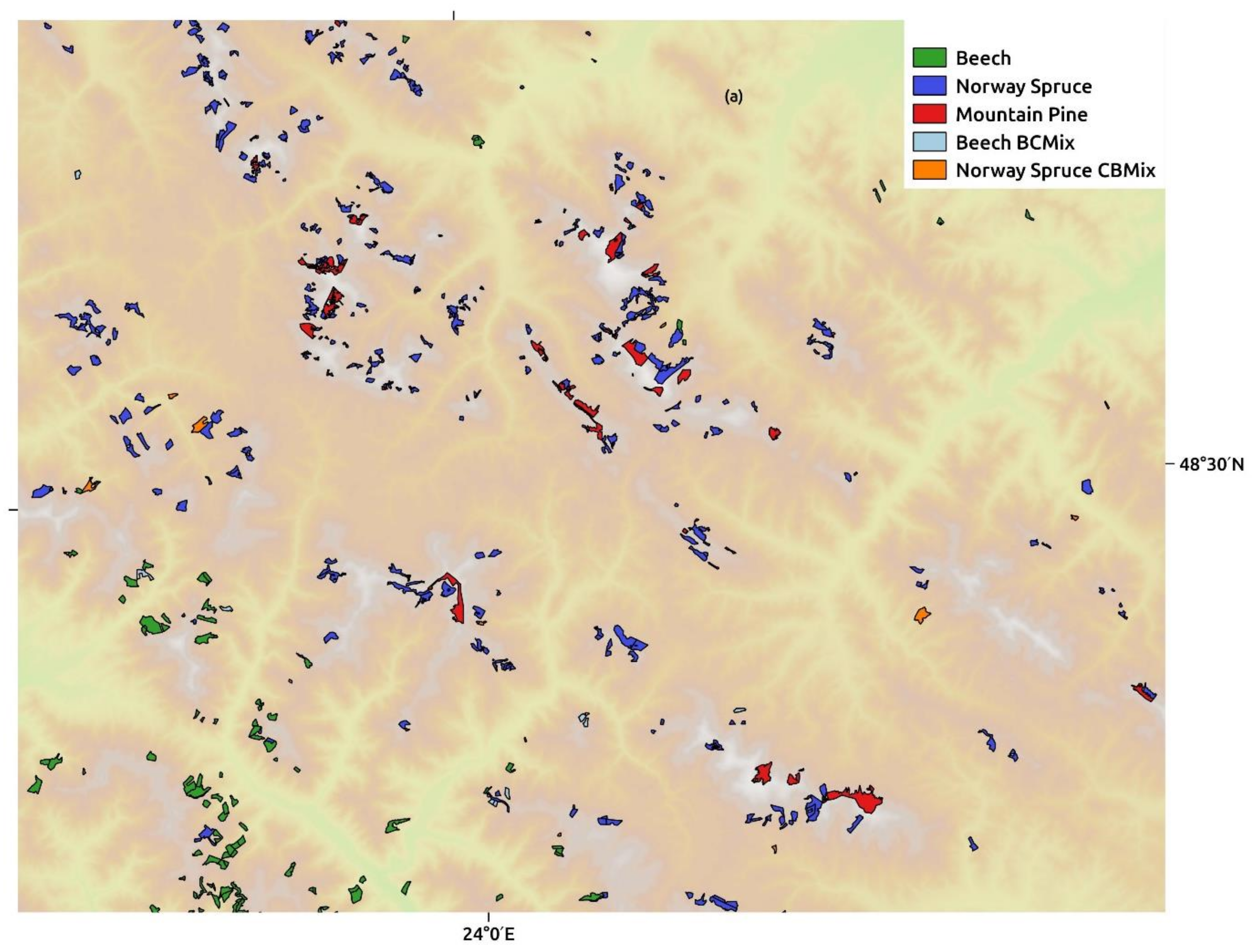
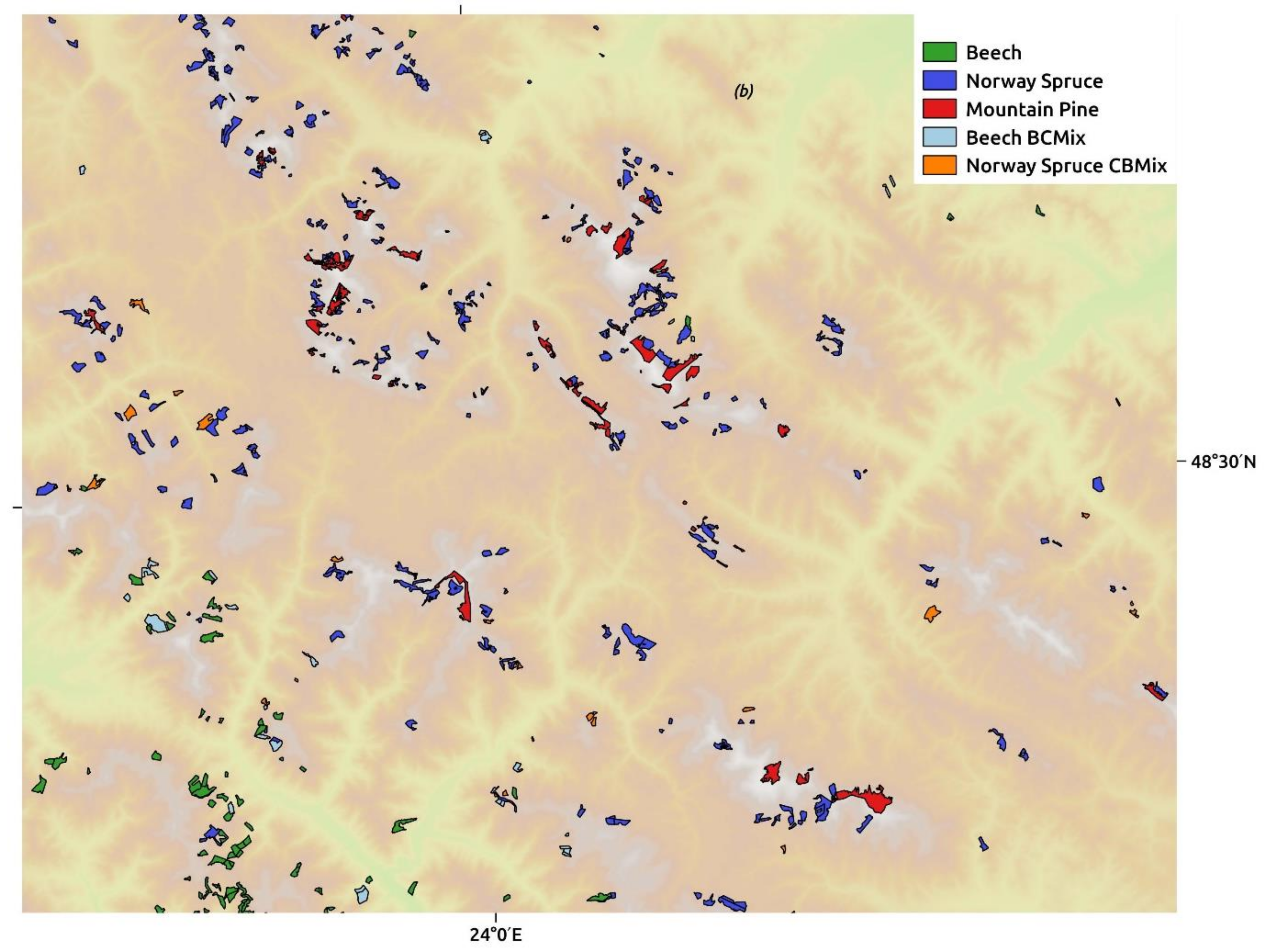
We first explored whether S2 images could be used to identify different tree species within OGF polygons. Figure S1 shows boxplots of all the spectral signatures, the vegetation indices and the textural measures of the various tree species, including oak and silver fir, for both summer and autumn The impact of autumnal colours for beech results in a 140% and 40% increase in brightness in the autumn red (B4) and red edge (B5) bands respectively compared to the summer bands (see Figure S1a). Land class maps are shown in Figure 2.
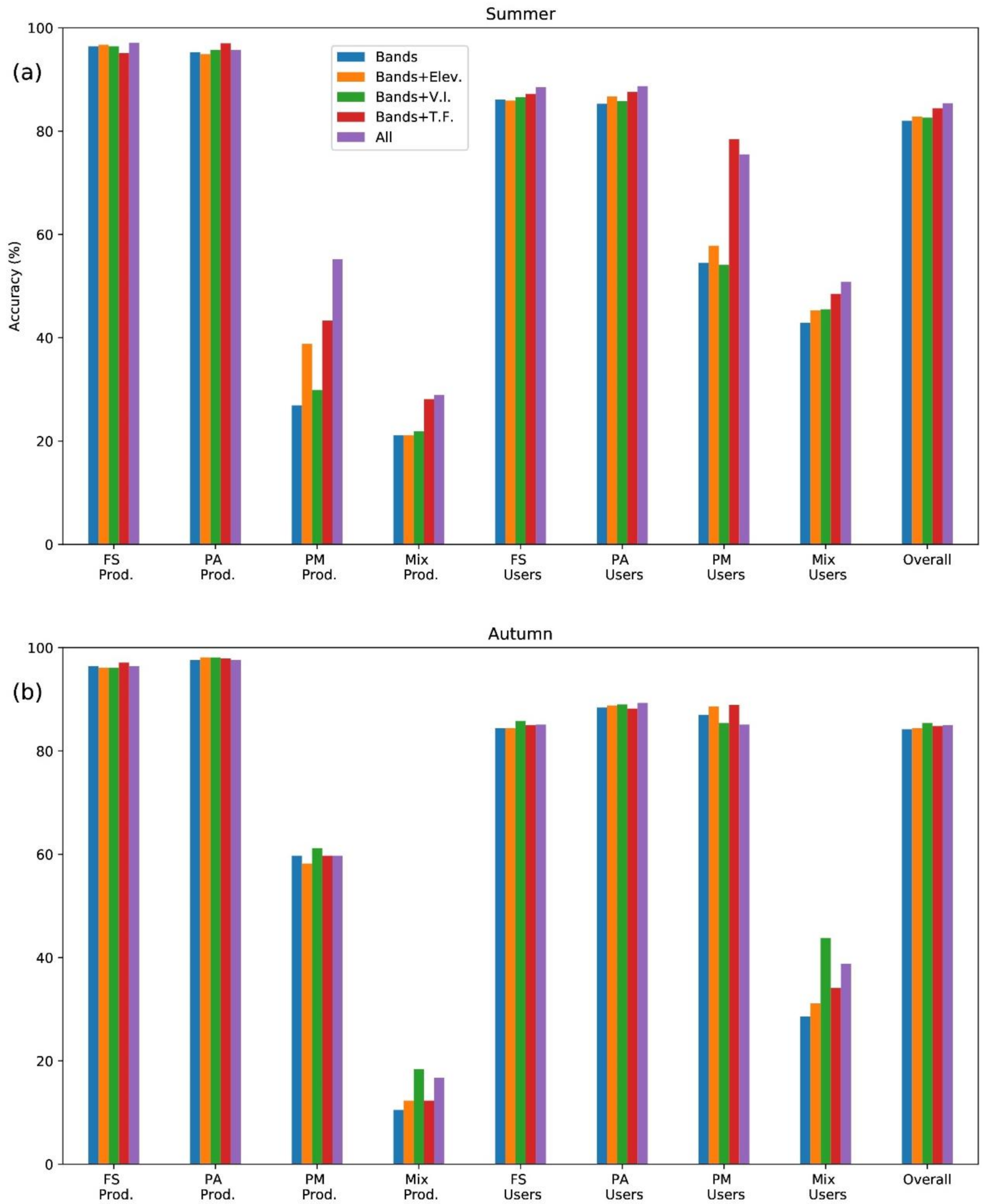
Figure S2 shows the ranking of features for importance. Figure 3 and Table S1 shows the classification accuracies for the tree species for summer and autumn images for the different Random Forest models. Beech and spruce consistently had the highest accuracies, with producer’s accuracy of 95%–98% and user’s accuracy of 85%–90%. Lower accuracy was achieved for mountain pine with producer’s accuracy of 25%–60% and user’s accuracy of 50%–90%. Classification was poorer for mixed forest with producer’s accuracy ranging from 10%–30% and user’s accuracy around 50%. For spruce and beech, producer’s accuracy was consistently higher than user’s accuracy, while for mixed and mountain pine the situation was reversed—a sign that the model was consistently misclassifying pine and mixed forest as spruce and beech. Similar remote sensing tree classification studies tend to obtain accuracies of between 70%–95% [15] and our study is generally in line with these.
In summer, SWIR, NIR and red edge bands (B5-7) were generally most important for classification (Table S1). Using only the bands, accuracy rates were higher using the autumn than the summer image by 2.2% (Figure 3)—the autumnal change in leaf colour was distinctive and consequently red and red edge bands were the best performing features for the autumn image (Table S1). Studies in eastern USA also found that mid-autumn was the best time for tree species classification [63,64]. For the summer image, adding elevation data improved overall accuracy. In particular, mountain pine, which only occurred at very high elevations in the study area, had its user’s and producer’s accuracy increased by 3.3% and 11.9% respectively. Previous studies have likewise found that topographic variables improved classification in studies in the USA [56,65] and Spain [56,65]. Vegetation indices performed better than the bands by 0.8% and 0.7% in summer and autumn respectively. Choice of features had a notable effect on accuracy for mountain pine, with user’s accuracy varying from 50% to 90%. Using combined summer and autumn images increased accuracy by 1.5%, less than the 2%–7% found by another study [60].
The Confusion matrix for the most accurate classification is shown in Table 4, with the diagonal cells showing the number (in bold) of correct classifications and the off-diagonal cells indicating the mistakes. In distinguishing beech and spruce it performed well, making just a single mistake and producer’s accuracies for these forest types was high (Figure 3). However, accuracy for mixed forests was poor, generally classing it as its pure tree species counterpart—i.e., beech mix was classed as pure beech and spruce mix as pure spruce. The model had trouble distinguishing between spruce and pine stands, classing 27 pine stands as spruce.
3.2. Distinguishing between OGF and non-OGF
Land class maps are shown in Figure 4. Figure S3 shows the mean spectral signatures, vegetation indices and textural measures for OGF and NOGF. OGF had a lower mean brightness than NOGF for both broadleaf and mixed forests over all bands in both summer and autumn. For broadleaf, t-tests showed a significant difference between OGF and NOGF for all non-visible bands (B5-B8, B8A, B11, B12) and all bands for summer and autumn images respectively (p < 0.05). For mixed forest, t-tests showed a significant difference (p < 0.05) between OGF and NOGF for all bands and all bands except blue (B2) for summer and autumn images respectively. Younger forests tend to consist of small tree crowns packed tightly together with few gaps. As the forest ages, both mean crown size and the number of gaps increases. The increase in forest gap number and shadows cast by emergent trees results in a reduction in the reflected light, leading to a lower mean brightness in OGF. Due to the inverse relation between wavelength and atmospheric scattering, shadows will be illuminated more by visible light (skylight) than longer wavelength bands [66,67]. Structurally diverse OGF would likely result in more shadows compared to NOGF, resulting in a larger difference between OGF and NOGF in the red edge, NIR and SWIR bands than the visible bands.
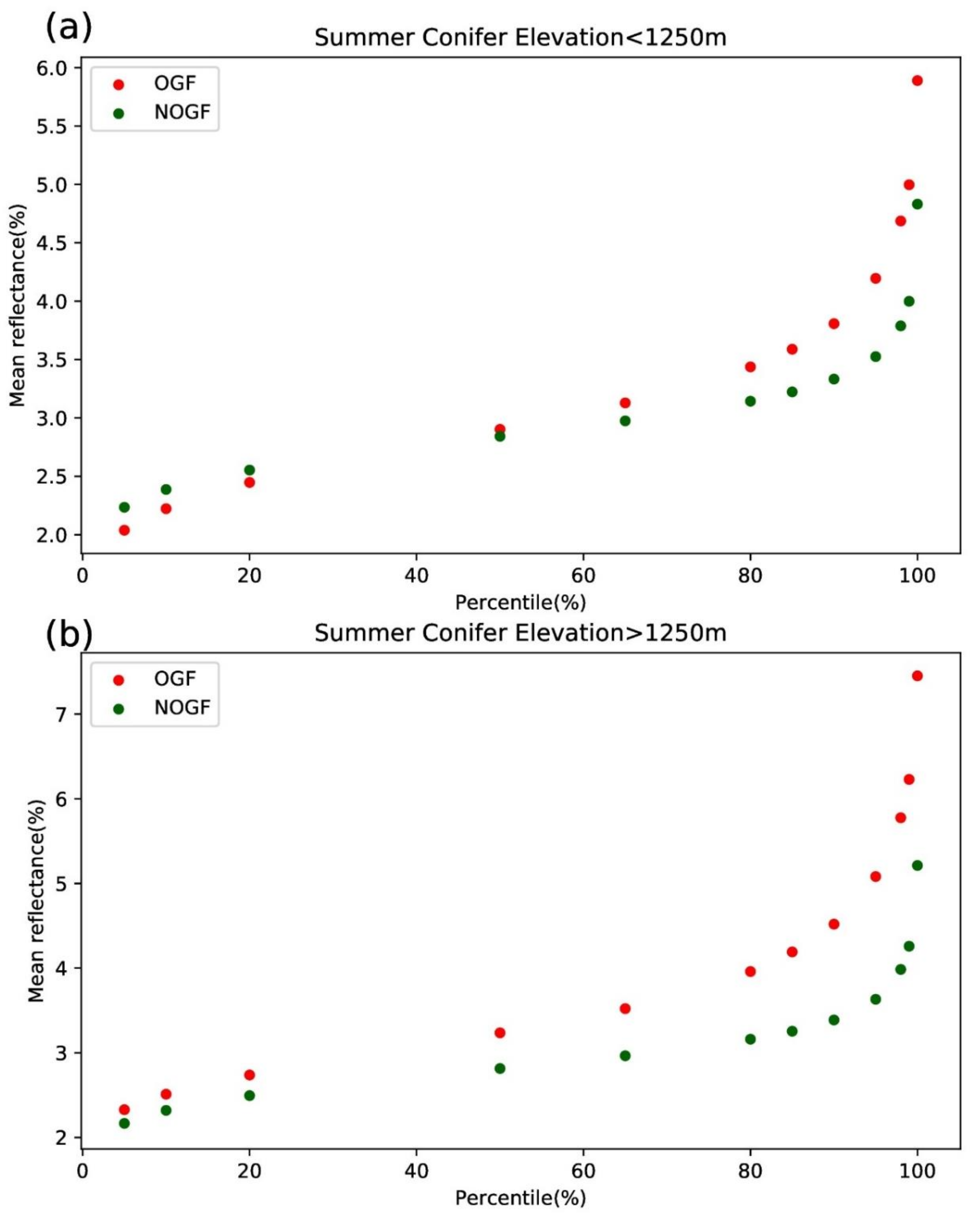
There was less difference between conifer OGF and conifer NOGF in the summer mean band spectra, with significantly higher reflectance in OGF for all bands except B7 (t-test, p < 0.05). This is a surprising result, as it is contrary both to the result for broadleaf and mixed forest, as well as to a previous study [21] which found conifer OGF significantly darker than mature forest in summer in blue, green and NIR Landsat bands. In our analysis, conifer OGF was, on average, at higher elevations compared to conifer NOGF (1341 m and 1237 m respectively). Therefore, it is likely that a higher percentage of conifer OGF consisted of mountain pine than in conifer NOGF and mountain pine was significantly brighter than Norway spruce and silver fir across all bands (see Figure S1). Furthermore, OGF towards the treeline was more likely to contain open forest and clearings than NOGF. If this were the case then the OGF image would contain many more bright pixels comprised of ground vegetation and soils. Open areas were generally about 50%–100% brighter than conifer canopy for all bands. To test if this difference could explain our surprising result, we plotted mean percentile values for OGF and NOGF conifers split into subsets of mean elevation above and below 1250 m (Figure 5). OGF conifer contained significantly more bright pixels (percentile > 80%) than NOGF and for OGF below 1250 m more dark pixels (percentile < 20%). In other words, the higher mean brightness of OGF was due to the presence of more bright pixels (open areas), while the wooded areas are darker than NOGF. (It is worth noticing that this pattern also holds true for broadleaf and mixed forest, as shown in Figure S4). OGF conifer with a mean elevation below 1250 m was significantly darker than NOGF for Bands B6-B8A. As conifer OGF increased in elevation, it contains more open ground (bright pixels), as can be seen from comparing Figure 5a,b. An alternative explanation we considered for this surprising result is that OGF conifer stands contain a higher percentage of broadleaved species (which are brighter across all bands) than NOGF conifer stands. However, in autumn the red (B4) band in conifer OGF and NOGF polygons brightens by about the same percentage relative to the summer image, so this is unlikely to be a factor.
The vegetation indices NDVI, AVI, RENDVI and EVI are strongly correlated to chlorophyll content [68,69]. All indices were greater for NOGF than OGF for all forest types (Figure S3b): as forest ages the amount of green vegetation tends to decline from both an increase in dead and dying trees and an increase in the amount of vegetation obscured by shadow from emergent trees. NDII is the difference index between the NIR and SWIR bands and a measure of the canopy water content [70]. It was likewise higher for NOGF than OGF for summer and autumn images, again attributable to greater non-photosynthetic vegetation in the OGF.
The texture of OGF was more heterogeneous, with OGF having higher contrast values for all images in all forest types and bands than NOGF (Figure S3c). The large crowns of OGF cast large shadows, which result in a coarse texture compare to the finer-grained texture of smaller, more densely packed, younger tree stands. In contrast to our results, an investigation [20] of the effects of stand structure on an absolute difference algorithm of tasselled cap vegetation indices found a poor correlation between these textural features and stand characteristics which included age, which the authors attribute to the coarse (30 m) resolution of the Landsat imagery used. A study of forest in Israel [51] found that contrary to our results, mature unmanaged forests had lower GLCM entropy and contrast values than younger forest. The authors explain this as resulting from the very high resolution (2 m) satellite imagery used, so that the large crown sizes associated with mature forest increased the number of adjacent pixels with similar grey levels.
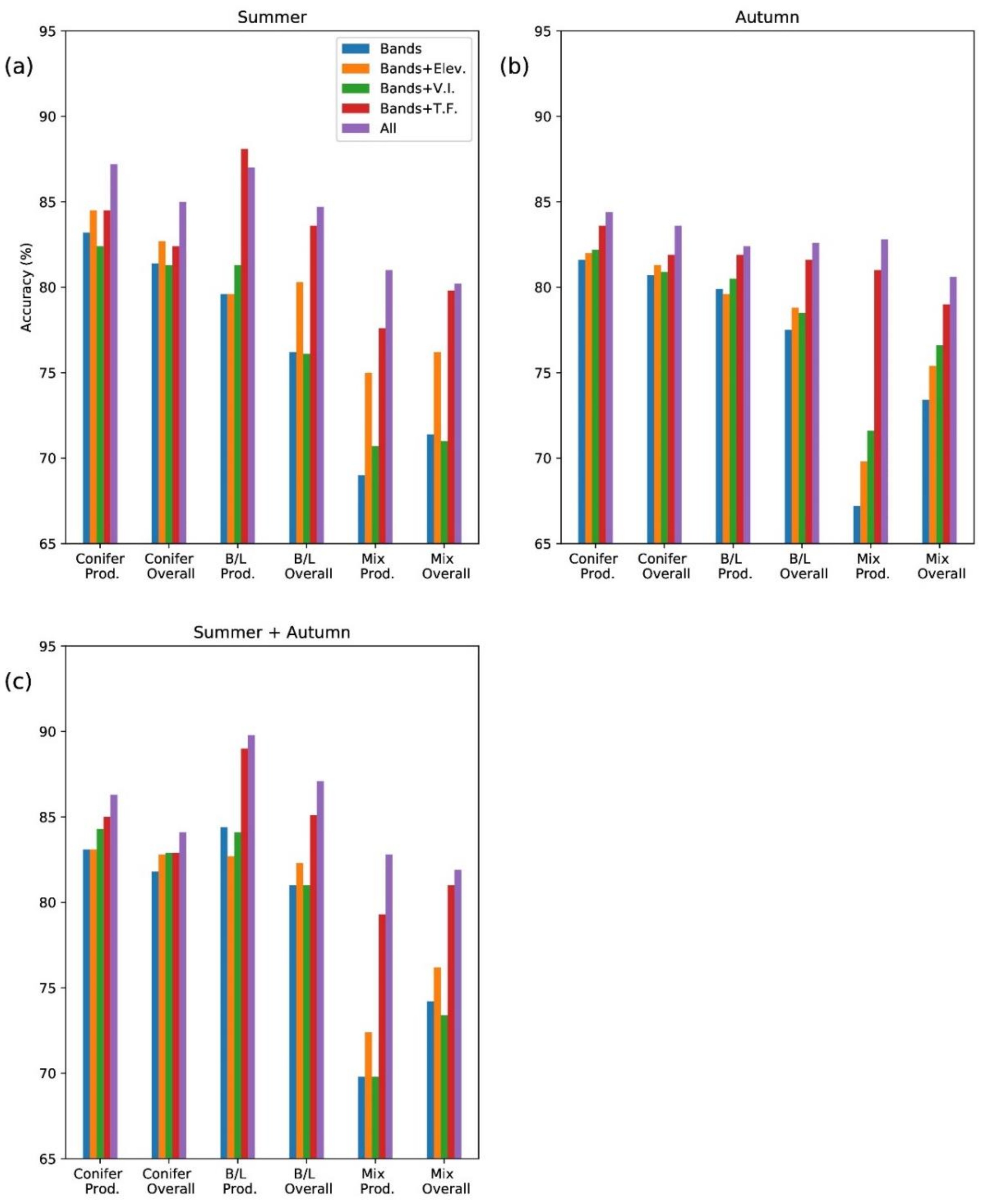
Figure 6 and Tables S2 and S3 shows the OGF producer’s accuracy and overall accuracy for Random Forest models. OGF producer’s accuracy is arguably the most important measure—it matters more if existing OGF is misidentified as NOGF and consequently overlooked than if we misclassify NOGF as OGF. Figure S5 shows the ranking of features for importance.
Classification accuracies for OGF were roughly uniform with both user’s and producer’s accuracies between 75%–85% for both conifer and broadleaf forest. Mixed forest accuracies were lower with producer’s accuracy ranging from 65%–80% and user’s accuracy around 70%–85%. Overall, classification accuracy using all features was 84%, on the verge of the 85% success threshold that is often used for machine learning studies. A previous study [19] obtained 75% accuracy in distinguishing OGF from mature forest using regression analysis and Landsat 5 imagery. Landsat 7 imagery and unsupervised classification was used [22] to distinguish old and mature conifer forests with an overall accuracy of 80%–90% depending on the ecoregion. Landsat 5 imagery and unsupervised classification [21] found 78% accuracy for classifying closed canopy conifer OGF. Another study [24] using Random Forest and high resolution LIDAR data to separate old near-natural and old managed conifer forest obtained overall classification accuracies of 85%–90%.
Accuracy was higher for mountain pine OGF stands than Norway spruce (about 92% and 83% respectively). This was consistent regardless of feature selection. Accuracy rose with elevation for both broadleaf and conifers. The model failed significantly with the small number of silver fir polygons—correctly identifying as OGF only about half. Again this result was consistent for all the RF models examined. For mixed forest the classification accuracy for Norway spruce CBMix was high (90%), while the accuracy for beech BCMix was much lower (70%).
A ranking of features (Table S2) indicates that in both summer and autumn, SWIR bands were most important for conifers, with red edge and NIR most important for broadleaves. Overall, for the band spectra accuracy rates were 0.3% higher using the summer than the autumn image. Adding elevation data to the bands usually improved overall accuracy (by an average of 1.8% overall): a large proportion of the surviving OGF ringed mountain summits, so that the adjacent NOGF polygons were generally lower in elevation.
Vegetation indices generally performed worse than Bands, with their use instead of bands reducing accuracy by 0.3%. Textural features performed extremely well and on average were 2.8% more accurate than just using the bands. Adding mean vegetation index, band standard deviations and textural feature data to the band spectra increased overall accuracy by 0.3%, 2.1% and 3.3% respectively (see Table S2 and Figure 6). Using all features improved accuracy by 5% compared to using just the mean band spectra.
We ran the RF classification separately on broadleaf, conifer and mixed forest types to provide insight into how performance and most important features differed for different forest types. However, the improvement in accuracy over running it on all OGF/NOGF forest types lumped together was fairly small (0.15%).
Figure 6 shows the producer’s overall accuracies for various season combinations using all features. Combining images improved accuracy in general, with the combined summer and autumn images 0.5% and 1.9% more accurate than summer or autumn on its own respectively. The highest overall accuracy achieved for all OGF polygons was 84.8% using summer and autumn images and all features.
4. Conclusions
The objective of this study was to evaluate the suitability of multitemporal Sentinel-2 data for identifying OGF tree species and distinguishing OGF from other woodland. The Sentinel-2 spectral signatures along with associated vegetation indices, textural features and elevation data were analysed with the Random Forest classifier. The OGF analysed consisted of beech, Norway spruce, mountain pine or mixtures of species in the Carpathian Mountains of Ukraine. An overall accuracy of about 85% was achieved in separating OGF from the surrounding forest, with classification accuracies higher for conifer and broadleaved than mixed forest.
We make a number of recommendations for automated identification of OGF. OGF is more spatially heterogeneous than other forest types. Adding textural features therefore improved classification. The addition of band standard deviations, combining summer and autumn images and adding elevation data also improved overall accuracy. We found limited benefits to using vegetation indices—which if added to the bands gave only a minimal performance improvement. We’d recommend calculating textural features instead as it involves the same amount of effort and since the spatial relationship of the pixels is not strongly correlated to their brightness you are adding useful independent information to the model.
Our method of comparing OGF to adjacent forest is not without weaknesses. It meant that our comparison of OGF to NOGF was not comparing ‘like-with-like,’ as the control NOGF polygons were usually forests lower in height. However, as remaining OGF in Europe is usually confined to the mountains this will tend to be true of any real-world attempt to classify OGF. Furthermore, ground identification will generally include criteria such as deadwood quantity and quality, presence of non-native tree species and human impact such as livestock grazing that cannot be surveyed remotely. With these caveats we were able to use free publicly available satellite imagery to correctly classify OGF on the ground with an overall accuracy of about 85%. This is at the threshold of what is usually deemed acceptable in machine learning studies [71]. Potential improvements could involve exploring the use of other classification types—for example, Support vector Machines (SVM) has been found to be more accurate than Random Forest in tree species classification studies [13,14,17]. Further studies that cover different OGF types within different biogeographical settings would be useful.
Supplementary Materials
The following are available online at https://0-www-mdpi-com.brum.beds.ac.uk/1999-4907/10/2/127/s1, Figure S1: Boxplots of (a) spectral signatures, (b) vegetation indices and (c) textural measures for tree species silver fir (AA), beech (FS), Norway spruce (PA), mountain pine (PM) and oak species (Quer) in Old-Growth Forest polygons, Figure S2: Random Forest feature importance for OGF tree species classification, Figure S3: Boxplots of (a) spectral signatures, (b) vegetation indices and (c) textural measures for broadleaf, conifer and mixed Old-Growth Forest and Non Old-Growth Forest polygons, arranged in two pairs of summer (thick line boxplots) and autumn (thin line boxplots) from left to right, Figure S4: Mean percentile values for the green Band (B3) for (a) broadleaf and (b) mixed Old-Growth Forest and Non-Old Growth Forest polygons, Figure S5: Random Forest feature importance for Old-Growth forest and Non-Old Growth forest classification for (a) conifers, (b) broadleaf, (c) mixed forest, Table S1: Producers, users and overall accuracy for Random Forest Old-Growth forest tree species classifications for our 8 models: mean band values (B), Textural features (TF), Vegetation indices(VI), B+TF, B+VI, B+mean elevation (elev), B+band standard deviations (B_sd) and B+B_sd+Elev+TF+VI, Table S2: Producers, users and overall accuracy for Random Forest Old Growth forest classification for our 8 models: mean band values (B), Textural features (TF), Vegetation indices(VI), B+TF, B+VI, B+mean elevation (elev), B+band standard deviations (B_sd) and B+B_sd+Elev+TF+VI, Table S3: Producers, users and overall accuracy for Random Forest Old-Growth Forest classification for summer and autumn images combined and our 8 models: mean band values (B), Textural features (TF), Vegetation indices(VI), B+TF, B+VI, B+mean elevation (elev), B+band standard deviations (B_sd) and B+B_sd+elev+TF+VI.
Author Contributions
Conceptualization, B.D.S. and D.V.S.; Methodology, B.D.S.; Software, B.D.S.; Validation, B.D.S.; Formal Analysis, B.D.S.; Investigation, B.D.S.; Resources, B.D.S. and D.V.S.; Data Curation, B.D.S.; Writing—Original Draft Preparation, B.D.S.; Writing—Review & Editing, D.V.S.; Visualization, B.D.S.; Supervision, D.V.S.; Project Administration, D.V.S.; Funding Acquisition, D.V.S.
Funding
We thank the United Bank of Carbon and the Natural Environment Research Council (NE/L013347/1) for funding. DVS acknowledges a Philip Leverhulme Prize.
Acknowledgments
We wish to thank WWF Ukraine and in particular Valeriia Nemykina, Taras Yamelynets and Roman Volosyanchuk for their assistance and provision of data. We thank three anonymous reviewers whose suggestions greatly improved the paper.
Conflicts of Interest
The authors declare no conflict of interest.
References
- Merce, O.; Borlea, G.F.; Turcu, D.O. Definitions and structural attributes of the ecosystems from natural forests-short review. J. Hortic. For. Biotechnol. 2014, 18, 114–120. [Google Scholar]
- Wirth, C.; Messier, C.; Bergeron, Y.; Frank, D.; Fankhänel, A. Old-growth forest definitions: A pragmatic view. Wirth, C., Gleixner, G., Heimann, M., Eds.; In Old-Growth Forests; Springer: Berlin/Heidelberg, Germany, 2009; Volume 207, pp. 11–33. [Google Scholar]
- Burrascano, S.; Keeton, W.S.; Sabatini, F.M.; Blasi, C. Commonality and variability in the structural attributes of moist temperate old-growth forests: A global review. For. Ecol. Manag. 2013, 291, 458–479. [Google Scholar] [CrossRef]
- Paillet, Y.; Bergès, L.; Hjältén, J.; Ódor, P.; Avon, C.; Bernhardt-Römermann, M.; Bijlsma, R.-J.; De Bruyn, L.U.C.; Fuhr, M.; Grandin, U.L.F.; et al. Biodiversity differences between managed and unmanaged forests: Meta-analysis of species richness in Europe. Conserv. Biol. 2010, 24, 101–112. [Google Scholar] [CrossRef] [PubMed]
- Granata, M.U.; Gratani, L.; Bracco, F.; Sartori, F.; Catoni, R. Carbon stock estimation in an unmanaged old-growth forest: A case study from a broad-leaf deciduous forest in the Northwest of Italy. Int. For. Rev. 2016, 18, 444–451. [Google Scholar] [CrossRef]
- Jacob, M.; Bade, C.; Calvete, H.; Dittrich, S.; Leuschner, C.; Hauck, M. Significance of over-mature and decaying trees for carbon stocks in a Central European natural spruce forest. Ecosystems 2013, 16, 336–346. [Google Scholar] [CrossRef]
- Seedre, M.; Kopáček, J.; Janda, P.; Bače, R.; Svoboda, M. Carbon pools in a montane old-growth Norway spruce ecosystem in Bohemian Forest: Effects of stand age and elevation. For. Ecol. Manag. 2015, 346, 106–113. [Google Scholar] [CrossRef]
- Keeton, W.S.; Chernyavskyy, M.; Gratzer, G.; Main-Knorn, M.; Shpylchak, M.; Bihun, Y. Structural characteristics and aboveground biomass of old-growth spruce–fir stands in the eastern Carpathian mountains, Ukraine. Plant Biosyst. 2010, 144, 148–159. [Google Scholar] [CrossRef]
- Luyssaert, S.; Schulze, E.-D.; Börner, A.; Knohl, A.; Hessenmöller, D.; Law, B.E.; Ciais, P.; Grace, J. Old-growth forests as global carbon sinks. Nature 2008, 455, 213–215. [Google Scholar] [CrossRef]
- Frey, S.J.; Hadley, A.S.; Johnson, S.L.; Schulze, M.; Jones, J.A.; Betts, M.G. Spatial models reveal the microclimatic buffering capacity of old-growth forests. Sci. Adv. 2016, 2, e1501392. [Google Scholar] [CrossRef]
- Sabatini, F.M.; Burrascano, S.; Keeton, W.S.; Levers, C.; Lindner, M.; Pötzschner, F.; Verkerk, P.J.; Bauhus, J.; Buchwald, E.; Chaskovsky, O.; et al. Where are Europe’s last primary forests? Divers. Distrib. 2018, 24, 1426–1439. [Google Scholar] [CrossRef]
- Knorn, J.A.N.; Kuemmerle, T.; Radeloff, V.C.; Keeton, W.S.; Gancz, V.; BIRIŞ, I.-A.; Svoboda, M.; Griffiths, P.; Hagatis, A.; Hostert, P. Continued loss of temperate old-growth forests in the Romanian Carpathians despite an increasing protected area network. Environ. Conserv. 2013, 40, 182–193. [Google Scholar] [CrossRef]
- Dalponte, M.; Bruzzone, L.; Gianelle, D. Tree species classification in the Southern Alps based on the fusion of very high geometrical resolution multispectral/hyperspectral images and LiDAR data. Remote Sens. Environ. 2012, 123, 258–270. [Google Scholar] [CrossRef]
- Heinzel, J.; Koch, B. Investigating multiple data sources for tree species classification in temperate forest and use for single tree delineation. Int. J. Appl. Earth Obs. Geoinf. 2012, 18, 101–110. [Google Scholar] [CrossRef]
- Immitzer, M.; Atzberger, C.; Koukal, T. Tree species classification with random forest using very high spatial resolution 8-band WorldView-2 satellite data. Remote Sens. 2012, 4, 2661–2693. [Google Scholar] [CrossRef]
- Puletti, N.; Chianucci, F.; Castaldi, C. Use of Sentinel-2 for forest classification in Mediterranean environments. Ann. Silvic. Res. 2018, 42, 32–38. [Google Scholar]
- Sheeren, D.; Fauvel, M.; Josipović, V.; Lopes, M.; Planque, C.; Willm, J.; Dejoux, J.-F. Tree species classification in temperate forests using Formosat-2 satellite image time series. Remote Sens. 2016, 8, 734. [Google Scholar] [CrossRef]
- Leckie, D.G.; Tinis, S.; Nelson, T.; Burnett, C.; Gougeon, F.A.; Cloney, E.; Paradine, D. Issues in species classification of trees in old growth conifer stands. Can. J. Remote Sens. 2005, 31, 175–190. [Google Scholar] [CrossRef]
- Cohen, W.B.; Spies, T.A.; Fiorella, M. Estimating the age and structure of forests in a multi-ownership landscape of western Oregon, USA. Int. J. Remote Sens. 1995, 16, 721–746. [Google Scholar] [CrossRef]
- Cohen, W.B.; Spies, T.A. Estimating structural attributes of Douglas-fir/western hemlock forest stands from Landsat and SPOT imagery. Remote Sens. Environ. 1992, 41, 1–17. [Google Scholar] [CrossRef]
- Fiorella, M.; Ripple, W.J. Determining successional stage of temperate coniferous forests with Landsat satellite data. Photogramm. Eng. Remote Sens. 1993, 59, 239–246. [Google Scholar]
- Jiang, H.; Strittholt, J.R.; Frost, P.A.; Slosser, N.C. The classification of late seral forests in the Pacific Northwest, USA using Landsat ETM+ imagery. Remote Sens. Environ. 2004, 91, 320–331. [Google Scholar] [CrossRef]
- Sabol Jr, D.E.; Gillespie, A.R.; Adams, J.B.; Smith, M.O.; Tucker, C.J. Structural stage in Pacific Northwest forests estimated using simple mixing models of multispectral images. Remote Sens. Environ. 2002, 80, 1–16. [Google Scholar] [CrossRef]
- Sverdrup-Thygeson, A.; Ørka, H.O.; Gobakken, T.; Næsset, E. Can airborne laser scanning assist in mapping and monitoring natural forests? For. Ecol. Manag. 2016, 369, 116–125. [Google Scholar] [CrossRef]
- Kathmann, F.; Ciutea, A.; Biris, I.-A.; Ibisch, P.L.; Salageanu, V. Potential Primary Forests Map of Romania; Ibisch, P.L., Ursu, A., Eds.; Greenpeace CEE Romania; Centre for Econics and Ecosystem Management, Eberswalde University for Sustainable Development; Geography Department, A. I. Cuza University of Iași: Bucharest, Romania, 2017; Available online: https://www.researchgate.net/publication/321098644_Potential_Primary_Forests_Map_of_Romania_published_by_Greenpeace_CEE_Romania_Centre_for_Econics_and_Ecosystem_Management_Eberswalde_University_for_Sustainable_Development_Geography_Department_A_I_Cuza (accessed on 11 January 2018).
- Immitzer, M.; Vuolo, F.; Atzberger, C. First experience with Sentinel-2 data for crop and tree species classifications in central Europe. Remote Sens. 2016, 8, 166. [Google Scholar] [CrossRef]
- Forest Code of Ukraine (in Ukrainian). Available online: https://zakon.rada.gov.ua/go/3852-12 (accessed on 10 January 2019).
- Lavnyy, V.; Lässig, R. Extent of storms in the Ukrainian Carpathians. In Proceedings of the Proceedings of the International Conference on Wind Effects on Trees, University of Karlsruhe, Karlsruhe, Baden-Württemberg, Germany, 16–18 September 2003; pp. 16–18. [Google Scholar]
- Simpson, M. Determining the potential distribution of highly invasive plants in the Carpathian Mountains of Ukraine: A species distribution modeling approach under different climate-land-use scenarios and possible implications for natural-resource management. Environ. Sci. Policy 2011, 12. Available online: http://0-jhir-library-jhu-edu.brum.beds.ac.uk/handle/1774.2/35707 (accessed on 10 January 2019).
- Kozak, J.; Estreguil, C.; Troll, M. Forest cover changes in the northern Carpathians in the 20th century: A slow transition. J. Land Use Sci. 2007, 2, 127–146. [Google Scholar] [CrossRef]
- Kuemmerle, T.; Hostert, P.; Radeloff, V.C.; van der Linden, S.; Perzanowski, K.; Kruhlov, I. Cross-border comparison of post-socialist farmland abandonment in the Carpathians. Ecosystems 2008, 11, 614. [Google Scholar] [CrossRef]
- Kuemmerle, T.; Hostert, P.; Radeloff, V.C.; Perzanowski, K.; Kruhlov, I. Post-socialist forest disturbance in the Carpathian border region of Poland, Slovakia and Ukraine. Ecol. Appl. 2007, 17, 1279–1295. [Google Scholar] [CrossRef]
- Kuemmerle, T.; Chaskovskyy, O.; Knorn, J.; Radeloff, V.C.; Kruhlov, I.; Keeton, W.S.; Hostert, P. Forest cover change and illegal logging in the Ukrainian Carpathians in the transition period from 1988 to 2007. Remote Sens. Environ. 2009, 113, 1194–1207. [Google Scholar] [CrossRef]
- Complicit in Corruption. How billion-dollar firms and EU Governments are Failing Ukraine’s Forests (2018) Earthsight. Available online: https://docs.wixstatic.com/ugd/624187_673e3aa69ed84129bdfeb91b6aa9ec17.pdf (accessed on 10 January 2019).
- Irland, L.; Kremenetska, E. Practical economics of forest ecosystem management: The case of the Ukrainian Carpathians. Ecol. Econ. Sustain. For. Manag. Dev. Trans-Discip. Approach Carpathian Mt. Ukr. Natl. For. Univ. Press 2009, 59, 180–200. [Google Scholar]
- Sitko, I.; Troll, M. Timberline changes in relation to summer farming in the Western Chornohora (Ukrainian Carpathians). Mt. Res. Dev. 2008, 28, 263–271. [Google Scholar] [CrossRef]
- Trotsiuk, V.; Hobi, M.L.; Commarmot, B. Age structure and disturbance dynamics of the relic virgin beech forest Uholka (Ukrainian Carpathians). For. Ecol. Manag. 2012, 265, 181–190. [Google Scholar] [CrossRef]
- Trotsiuk, V.; Svoboda, M.; Janda, P.; Mikolas, M.; Bace, R.; Rejzek, J.; Samonil, P.; Chaskovskyy, O.; Korol, M.; Myklush, S. A mixed severity disturbance regime in the primary Picea abies (L.) Karst. forests of the Ukrainian Carpathians. For. Ecol. Manag. 2014, 334, 144–153. [Google Scholar] [CrossRef]
- Hobi, M.L.; Commarmot, B.; Bugmann, H. Pattern and process in the largest primeval beech forest of E urope (Ukrainian Carpathians). J. Veg. Sci. 2015, 26, 323–336. [Google Scholar] [CrossRef]
- Volosyanchuk, R.; Prots, B.; Kagalo, A.; Shparyk, Y.; Cherniavskyi, M.; Bondaruk, G. Criteria and Methology for Virgin and Old-Growth (Quasi-Virgin) Forest Identification; Volosyanchuk, R., Prots, B., Kagalo, A., Eds.; Liga Press: Lviv, Ukraine, 2017. Available online: http://d2ouvy59p0dg6k.cloudfront.net/downloads/old_growth_forest_identification_methodology.pdf (accessed on 1 December 2018).
- Roman Volosyanchuk Virgin and Old Growth Forests in Ukraine. Available online: http://www.carpathianconvention.org/tl_files/carpathiancon/Downloads/03%20Meetings%20and%20Events/Working%20Groups/Sustainable%20Forest%20Management/6th%20meeting/presentations/VF_for_CC_Sopron_WWF_UA.pdf (accessed on 11 January 2018).
- Hansen, M.C.; Potapov, P.V.; Moore, R.; Hancher, M.; Turubanova, S.A.; Tyukavina, A.; Thau, D.; Stehman, S.V.; Goetz, S.J.; Loveland, T.R.; et al. High-resolution global maps of 21st-century forest cover change. Science 2013, 342, 850–853. [Google Scholar] [CrossRef] [PubMed]
- Wulder, M.A.; Skakun, R.S.; Kurz, W.A.; White, J.C. Estimating time since forest harvest using segmented Landsat ETM+ imagery. Remote Sens. Environ. 2004, 93, 179–187. [Google Scholar] [CrossRef]
- Drusch, M.; Del Bello, U.; Carlier, S.; Colin, O.; Fernandez, V.; Gascon, F.; Hoersch, B.; Isola, C.; Laberinti, P.; Martimort, P. Sentinel-2: ESA’s optical high-resolution mission for GMES operational services. Remote Sens. Environ. 2012, 120, 25–36. [Google Scholar] [CrossRef]
- Louis, J.; Debaecker, V.; Pflug, B.; Main-Knorn, M.; Bieniarz, J.; Mueller-Wilm, U.; Cadau, E.; Gascon, F. Sentinel-2 Sen2Cor: L2A Processor for Users. In Proceedings of the Proceedings Living Planet Symposium 2016, Prague, Czech Republic, 9–13 May 2016; pp. 1–8. [Google Scholar]
- Clark, M.L.; Roberts, D.A.; Clark, D.B. Hyperspectral discrimination of tropical rain forest tree species at leaf to crown scales. Remote Sens. Environ. 2005, 96, 375–398. [Google Scholar] [CrossRef]
- Coburn, C.A.; Roberts, A.C. A multiscale texture analysis procedure for improved forest stand classification. Int. J. Remote Sens. 2004, 25, 4287–4308. [Google Scholar] [CrossRef]
- Zhaoa, P.; Zhaoa, J.; Wub, J.; Yanga, Y.; Xuea, W.; Houa, Y. Integration of multi-classifiers in object-based methods for forest classification in the Loess plateau, China. SCIENCEASIA 2016, 42, 283–289. [Google Scholar] [CrossRef]
- Haralick, R.M. Statistical and structural approaches to texture. Proc. IEEE 1979, 67, 786–804. [Google Scholar] [CrossRef]
- Hall-Beyer, M. GLCM Texture: A Tutorial; Technical Report for Department of Geography; University of Calgary: Calgary, AB, Canada, March 2000. [Google Scholar]
- Ozdemir, I.; Karnieli, A. Predicting forest structural parameters using the image texture derived from WorldView-2 multispectral imagery in a dryland forest, Israel. Int. J. Appl. Earth Obs. Geoinf. 2011, 13, 701–710. [Google Scholar] [CrossRef]
- Shaban, M.A.; Dikshit, O. Improvement of classification in urban areas by the use of textural features: The case study of Lucknow city, Uttar Pradesh. Int. J. Remote Sens. 2001, 22, 565–593. [Google Scholar] [CrossRef]
- Chen, D.; Stow, D.A.; Gong, P. Examining the effect of spatial resolution and texture window size on classification accuracy: An urban environment case. Int. J. Remote Sens. 2004, 25, 2177–2192. [Google Scholar] [CrossRef]
- Jarvis, A.; Reuter, H.I.; Nelson, A.; Guevara, E. Hole-filled SRTM for the globe Version 4: Data grid. 2008. Available online: https://research.utwente.nl/en/publications/hole-filled-srtm-for-the-globe-version-4-data-grid (accessed on 31 December 2018).
- Breiman, L. Random forests. Mach. Learn. 2001, 45, 5–32. [Google Scholar] [CrossRef]
- Rodriguez-Galiano, V.F.; Ghimire, B.; Rogan, J.; Chica-Olmo, M.; Rigol-Sanchez, J.P. An assessment of the effectiveness of a random forest classifier for land-cover classification. ISPRS J. Photogramm. Remote Sens. 2012, 67, 93–104. [Google Scholar] [CrossRef]
- Cutler, D.R.; Edwards Jr, T.C.; Beard, K.H.; Cutler, A.; Hess, K.T.; Gibson, J.; Lawler, J.J. Random forests for classification in ecology. Ecology 2007, 88, 2783–2792. [Google Scholar] [CrossRef] [PubMed]
- Pal, M. Random forest classifier for remote sensing classification. Int. J. Remote Sens. 2005, 26, 217–222. [Google Scholar] [CrossRef]
- Sesnie, S.E.; Finegan, B.; Gessler, P.E.; Thessler, S.; Ramos Bendana, Z.; Smith, A.M. The multispectral separability of Costa Rican rainforest types with support vector machines and Random Forest decision trees. Int. J. Remote Sens. 2010, 31, 2885–2909. [Google Scholar] [CrossRef]
- Nelson, M. Evaluating Multitemporal Sentinel-2 data for Forest Mapping using Random Forest. Master’s Thesis, Stockholm University, Stockholm, Sweden, December 2017. [Google Scholar]
- Pedregosa, F.; Varoquaux, G.; Gramfort, A.; Michel, V.; Thirion, B.; Grisel, O.; Blondel, M.; Prettenhofer, P.; Weiss, R.; Dubourg, V. Scikit-learn: Machine learning in Python. J. Mach. Learn. Res. 2011, 12, 2825–2830. [Google Scholar]
- Lu, D.; Weng, Q. A survey of image classification methods and techniques for improving classification performance. Int. J. Remote Sens. 2007, 28, 823–870. [Google Scholar] [CrossRef]
- Key, T.; Warner, T.A.; McGraw, J.B.; Fajvan, M.A. A comparison of multispectral and multitemporal information in high spatial resolution imagery for classification of individual tree species in a temperate hardwood forest. Remote Sens. Environ. 2001, 75, 100–112. [Google Scholar] [CrossRef]
- Schriever, J.R.; Congalton, R.G. Evaluating seasonal variablity as an aid to cover-type mapping from landsat thematic mapper data in the northwest. Photogramm. Eng. Remote Sens. 1995, 61, 321–327. [Google Scholar]
- Zimmermann, N.E.; Edwards, T.C.; Moisen, G.G.; Frescino, T.S.; Blackard, J.A. Remote sensing-based predictors improve distribution models of rare, early successional and broadleaf tree species in Utah. J. Appl. Ecol. 2007, 44, 1057–1067. [Google Scholar] [CrossRef] [PubMed]
- Crist, E.P.; Laurin, R.; Cicone, R.C. Vegetation and soils information contained in transformed Thematic Mapper data. In Proceedings of the Proceedings of IGARSS’86 Symposium; European Space Agency: Paris, France, 1986; pp. 1465–1470. [Google Scholar]
- Kimes, D.S.; Newcomb, W.W.; Nelson, R.F.; Schutt, J.B. Directional reflectance distributions of a hardwood and pine forest canopy. IEEE Trans. Geosci. Remote Sens. 1986, 24, 281–293. [Google Scholar] [CrossRef]
- Glenn, E.; Huete, A.; Nagler, P.; Nelson, S. Relationship between remotely-sensed vegetation indices, canopy attributes and plant physiological processes: What vegetation indices can and cannot tell us about the landscape? Sensors 2008, 8, 2136–2160. [Google Scholar] [CrossRef] [PubMed]
- Tuominen, J.; Lipping, T.; Kuosmanen, V.; Haapanen, R. Remote Sensing of Forest Health. Geoscience and Remote Sensing; IntechOpen: London, UK, 2009; Available online: https://www.intechopen.com/books/geoscience-and-remote-sensing/remote-sensing-of-forest-health (accessed on 1 January 2019).
- Yilmaz, M.T.; Hunt, E.R., Jr.; Goins, L.D.; Ustin, S.L.; Vanderbilt, V.C.; Jackson, T.J. Vegetation water content during SMEX04 from ground data and Landsat 5 Thematic Mapper imagery. Remote Sens. Environ. 2008, 112, 350–362. [Google Scholar] [CrossRef]
- Thomlinson, J.R.; Bolstad, P.V.; Cohen, W.B. Coordinating methodologies for scaling landcover classifications from site-specific to global: Steps toward validating global map products. Remote Sens. Environ. 1999, 70, 16–28. [Google Scholar] [CrossRef]
Figure 1.
Relief map (elevation range 200–2060 m) of the study site showing Old-Growth Forest (OGF, shown as red polygons) and Non-Old Growth Forest (NOGF, shown as blue polygons). S2 image shows the extent of the Sentinel-2 image used in the study. Inset map shows the location of the study area within Ukraine.

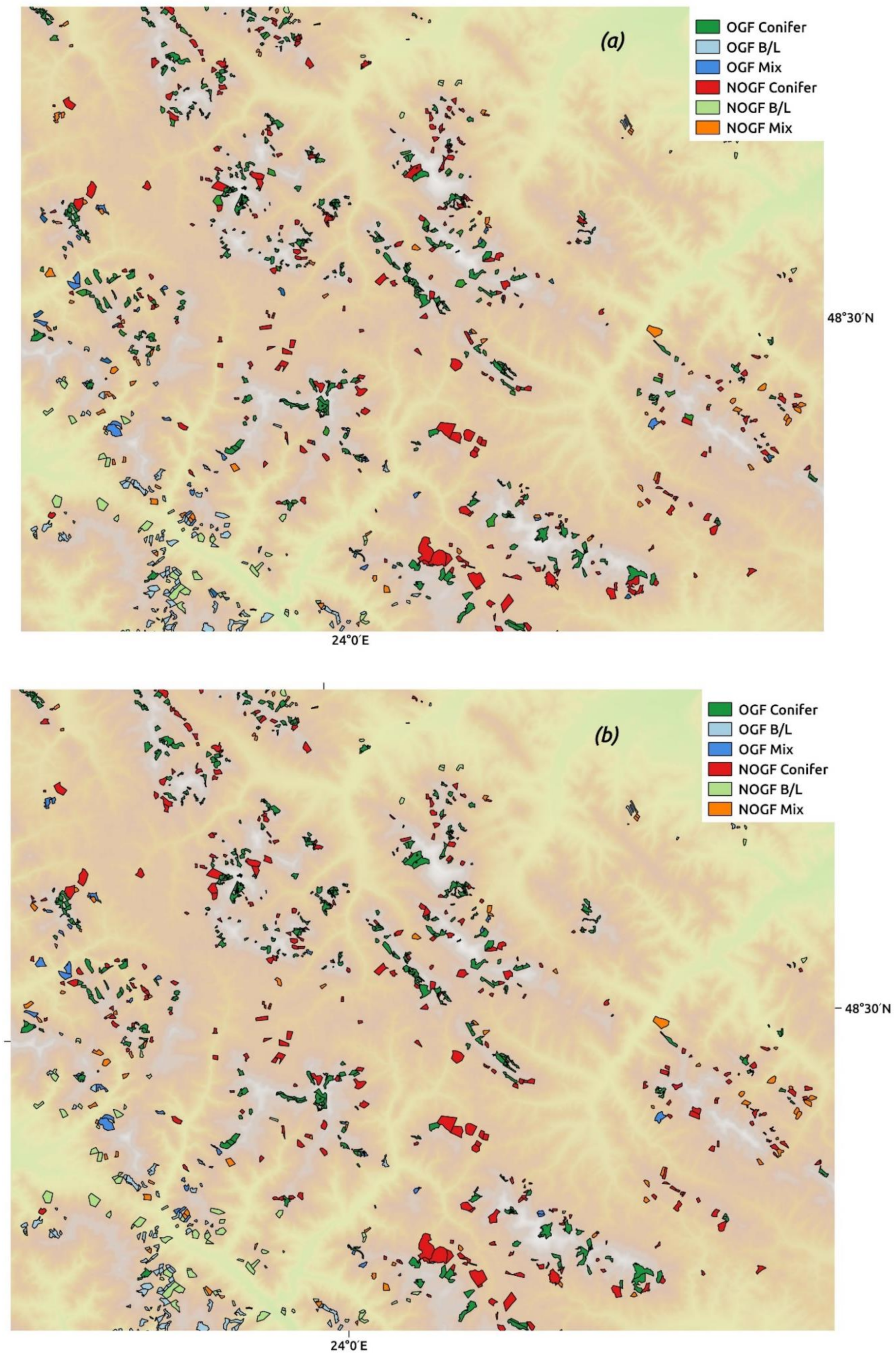
Figure 2.
Map of Old-Growth Forest tree species based on (a) the Random Forest classifier using all features for combined summer and autumn images (b) WWF ground survey. Beech BCMix is dominant beech with at least 20% conifer species, Norway Spruce CBMix is dominant Norway spruce with at least 20% broadleaf species.


Figure 3.
User’s, producer’s and overall accuracies resulting from Random Forest classification for Old-Growth Forest tree species for 5 selected models in (a) Summer (2 August 2017) and (b) Autumn (16 October 2017). Abbreviations: FS—Beech, PA—Norway spruce, PM—mountain pine.
Figure 3.
User’s, producer’s and overall accuracies resulting from Random Forest classification for Old-Growth Forest tree species for 5 selected models in (a) Summer (2 August 2017) and (b) Autumn (16 October 2017). Abbreviations: FS—Beech, PA—Norway spruce, PM—mountain pine.

Figure 4.
Map of Old-Growth Forest and Non-Old-Growth Forest based on (a) the Random Forest classifier using all features for combined summer and autumn images (b) the WWF ground survey.
Figure 4.
Map of Old-Growth Forest and Non-Old-Growth Forest based on (a) the Random Forest classifier using all features for combined summer and autumn images (b) the WWF ground survey.

Figure 5.
Mean percentile values for the green Band (B3) for conifer Old-Growth Forest and non-Old-Growth Forest polygons with mean elevation (a) below 1250 m (b) above 1250 m.
Figure 5.
Mean percentile values for the green Band (B3) for conifer Old-Growth Forest and non-Old-Growth Forest polygons with mean elevation (a) below 1250 m (b) above 1250 m.

Figure 6.
Old-Growth Forest (OGF) Producer’s and overall accuracies resulting from Random Forest classification for OGF and Non-OGF polygons for 5 selected models for (a) summer (2 August 2017) (b) autumn (16 October 2017) and (c) summer + autumn.
Figure 6.
Old-Growth Forest (OGF) Producer’s and overall accuracies resulting from Random Forest classification for OGF and Non-OGF polygons for 5 selected models for (a) summer (2 August 2017) (b) autumn (16 October 2017) and (c) summer + autumn.


Table 1.
Number and area of polygons used in this study (not including polygons damaged by man) for different tree species in OGF polygons. We denoted mixed tree species polygons as “Dominant Tree Species Mix,” while C and B stand for conifer and broadleaved respectively. Thus, Norway Spruce CBMix is Norway spruce dominant mixed with at least 20% broadleaved species, while Beech BMix is beech dominated mixed with at least 20% other broadleaved species.
| Tree Species | Number of Polygons | Area (km2) | Mean Elev (m) | Min Elev (m) | Max. Elev (m) | Mean Slope (o) |
|---|---|---|---|---|---|---|
| Beech | 1281 | 139.2 | 1055 | 394 | 1565 | 24.2 |
| Oak | 21 | 3.2 | 507 | 334 | 871 | 13.2 |
| Mountain Pine | 219 | 37.4 | 1477 | 1061 | 1982 | 22 |
| Norway Spruce | 1784 | 182.4 | 1343 | 519 | 1688 | 22.1 |
| Silver Fir | 20 | 1.3 | 598 | 481 | 946 | 12.5 |
| Beech BCMix | 189 | 16.0 | 1052 | 425 | 1443 | 24.5 |
| Norway Spruce CBMix | 226 | 19.2 | 1136 | 514 | 1620 | 29.2 |
| Silver Fir CBMix | 60 | 5.3 | 933 | 515 | 1286 | 24.8 |
| Beech BMix | 59 | 5.1 | 1039 | 454 | 1497 | 26.1 |
| Other Bmix | 15 | 1.5 | 618 | 342 | 1131 | 14 |
| Other BCMix | 6 | 0.7 | 1410 | 1030 | 1719 | 21.2 |
| Norway Spruce CMix | 98 | 10.6 | 1266 | 703 | 1568 | 22.3 |
| Other CMix | 48 | 6.0 | 1209 | 591 | 1953 | 23.1 |
| Other CBMix | 2 | 0.1 | 1598 | 1374 | 1722 | 24 |
| Other B | 2 | 0.07 | 1522 | 1422 | 1633 | 31.2 |
| Other C | 4 | 0.15 | 929 | 733 | 1373 | 24.5 |
| Total Conifer | 2173 | 237.6 | 1341 | 481 | 1982 | 22 |
| Total Broadleaf | 1378 | 149 | 1042 | 334 | 1633 | 24 |
| Total Mixed | 486 | 41.4 | 1084 | 342 | 1689 | 24.3 |
| Total | 4037 | 428 | 1208 | 334 | 1982 | 23 |
Table 2.
Number and area of polygons used in this study for different forest types in non-OGF polygons.
Table 2.
Number and area of polygons used in this study for different forest types in non-OGF polygons.
| Forest Type | Number of Polygons | Area (km2) | Mean Elev. (m) | Min Elev. (m) | Max Elev. (m) | Mean Slope (o) |
|---|---|---|---|---|---|---|
| Conifer | 2563 | 299.6 | 1238 | 457 | 1792 | 20.2 |
| Broadleaved | 1343 | 206.1 | 888 | 357 | 1456 | 23.6 |
| Mixed | 543 | 57.5 | 1045 | 438 | 1566 | 22.9 |
| Total | 4449 | 560.5 | 1108 | 357 | 1792 | 21.5 |
Table 3.
Sentinel-2 bands with 10 m or 20 m resolution. Near IR is Near Infra-Red and SWIR is Short wave Infra-Red.
Table 3.
Sentinel-2 bands with 10 m or 20 m resolution. Near IR is Near Infra-Red and SWIR is Short wave Infra-Red.
| Sentinel-2 Bands | Central Wavelength (µm) | Resolution (m) |
|---|---|---|
| B2–Blue | 0.490 | 10 |
| B3–Green | 0.560 | 10 |
| B4-Red | 0.665 | 10 |
| B5–Red edge | 0.705 | 20 |
| B6–Red edge | 0.740 | 20 |
| B7–Red edge | 0.783 | 20 |
| B8–Near IR | 0.842 | 10 |
| B8A–Near IR | 0.865 | 20 |
| B11–SWIR | 1.610 | 20 |
| B12–SWIR | 2.190 | 20 |
Table 4.
Confusion matrix for three dominant tree species plus FS mix with conifers and PA mix with broadleaved, based on the most accurate Random Forest classification—summer and autumn mean band spectra with all features. FS—beech, PA—Norway spruce, PM—mountain pine.
Table 4.
Confusion matrix for three dominant tree species plus FS mix with conifers and PA mix with broadleaved, based on the most accurate Random Forest classification—summer and autumn mean band spectra with all features. FS—beech, PA—Norway spruce, PM—mountain pine.
| Predicted Species | |||||||
|---|---|---|---|---|---|---|---|
| FS | FS mix | PM | PA | PA mix | Sum | ||
| Actual species | FS | 300 | 5 | 0 | 0 | 4 | 309 |
| FS mix | 36 | 9 | 0 | 0 | 5 | 50 | |
| PM | 0 | 0 | 40 | 27 | 0 | 67 | |
| PA | 1 | 1 | 3 | 460 | 3 | 468 | |
| PA mix | 8 | 6 | 1 | 27 | 22 | 64 | |
| Sum | 345 | 21 | 44 | 514 | 34 | 958 | |
© 2019 by the authors. Licensee MDPI, Basel, Switzerland. This article is an open access article distributed under the terms and conditions of the Creative Commons Attribution (CC BY) license (http://creativecommons.org/licenses/by/4.0/).
Share and Cite
MDPI and ACS Style
Spracklen, B.D.; Spracklen, D.V. Identifying European Old-Growth Forests using Remote Sensing: A Study in the Ukrainian Carpathians. Forests 2019, 10, 127. https://0-doi-org.brum.beds.ac.uk/10.3390/f10020127
AMA Style
Spracklen BD, Spracklen DV. Identifying European Old-Growth Forests using Remote Sensing: A Study in the Ukrainian Carpathians. Forests. 2019; 10(2):127. https://0-doi-org.brum.beds.ac.uk/10.3390/f10020127
Chicago/Turabian StyleSpracklen, Benedict D., and Dominick V. Spracklen. 2019. "Identifying European Old-Growth Forests using Remote Sensing: A Study in the Ukrainian Carpathians" Forests 10, no. 2: 127. https://0-doi-org.brum.beds.ac.uk/10.3390/f10020127
Note that from the first issue of 2016, this journal uses article numbers instead of page numbers. See further details here.