Impact of Large-Scale Afforestation on Surface Temperature: A Case Study in the Kubuqi Desert, Inner Mongolia Based on the WRF Model

 , ,
, ,
Abstract
:1. Introduction
2. Methods
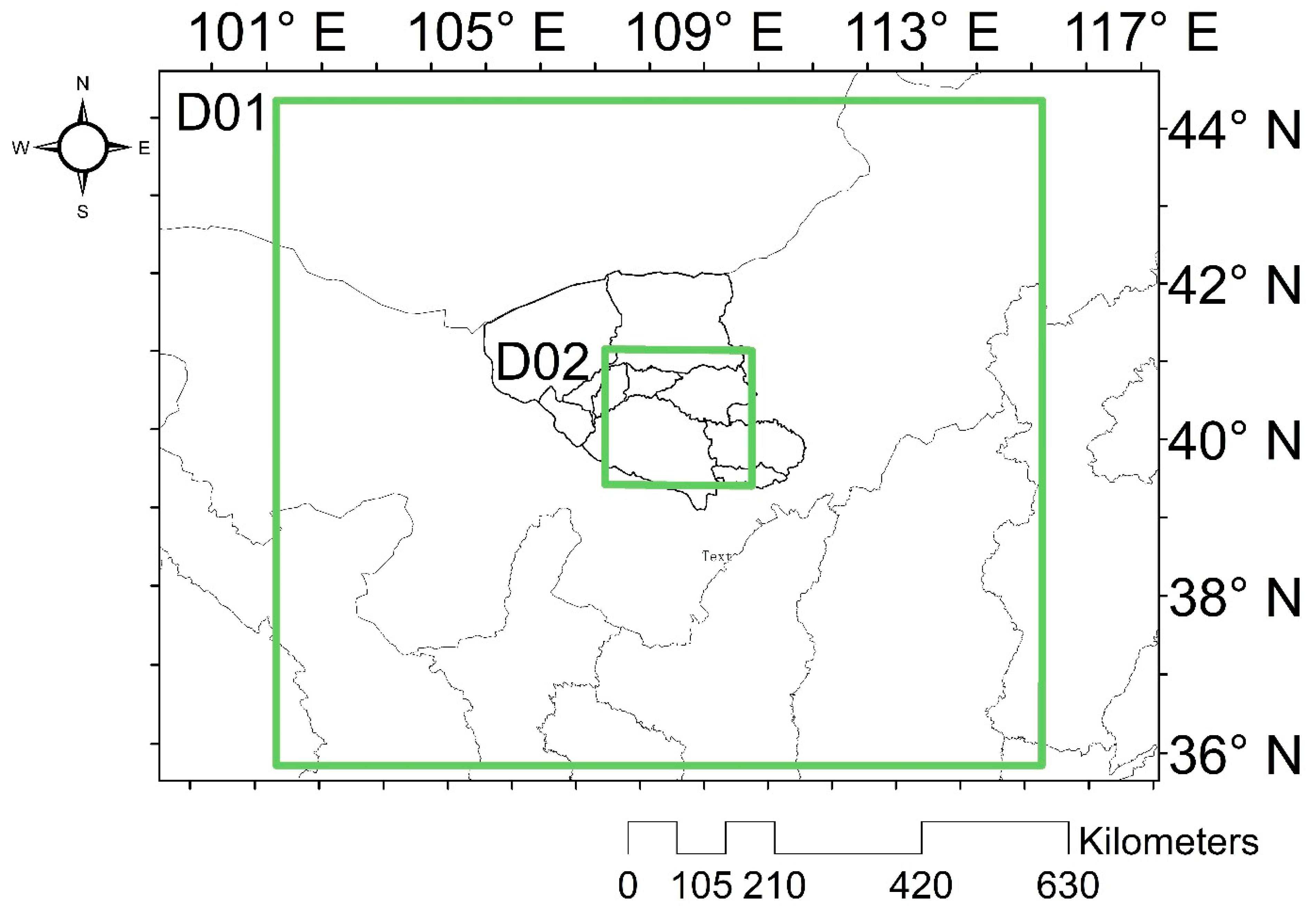
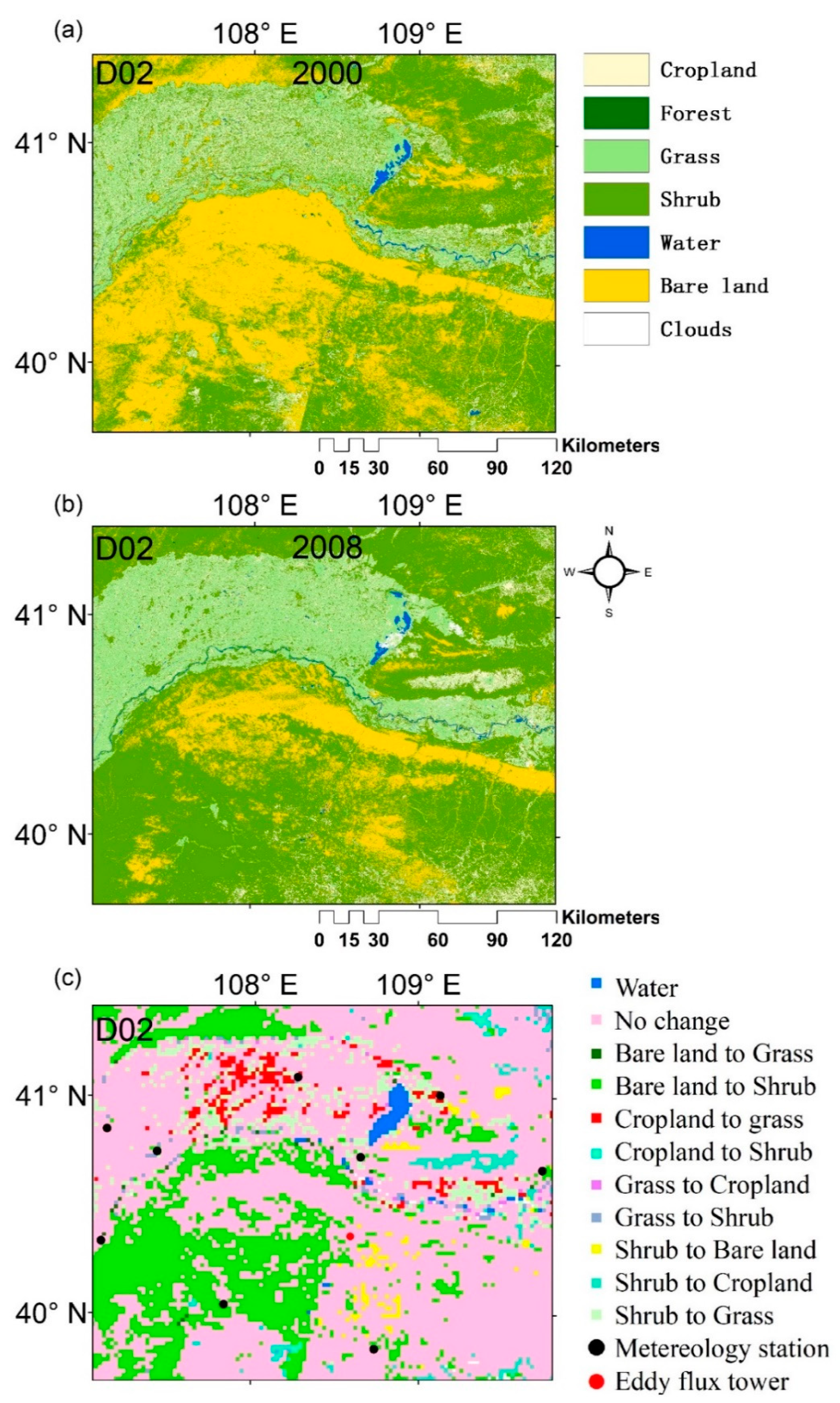
2.1. WRF Modeling
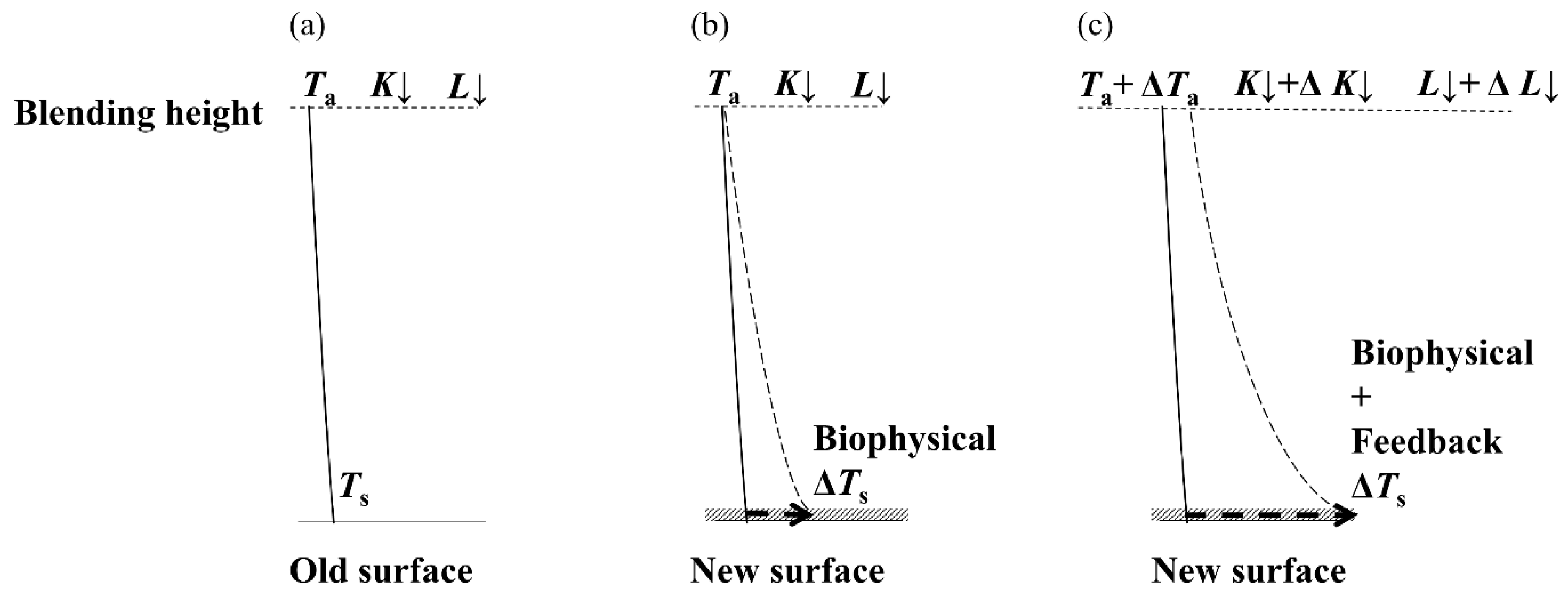
2.2. Offline Calculations
3. Results
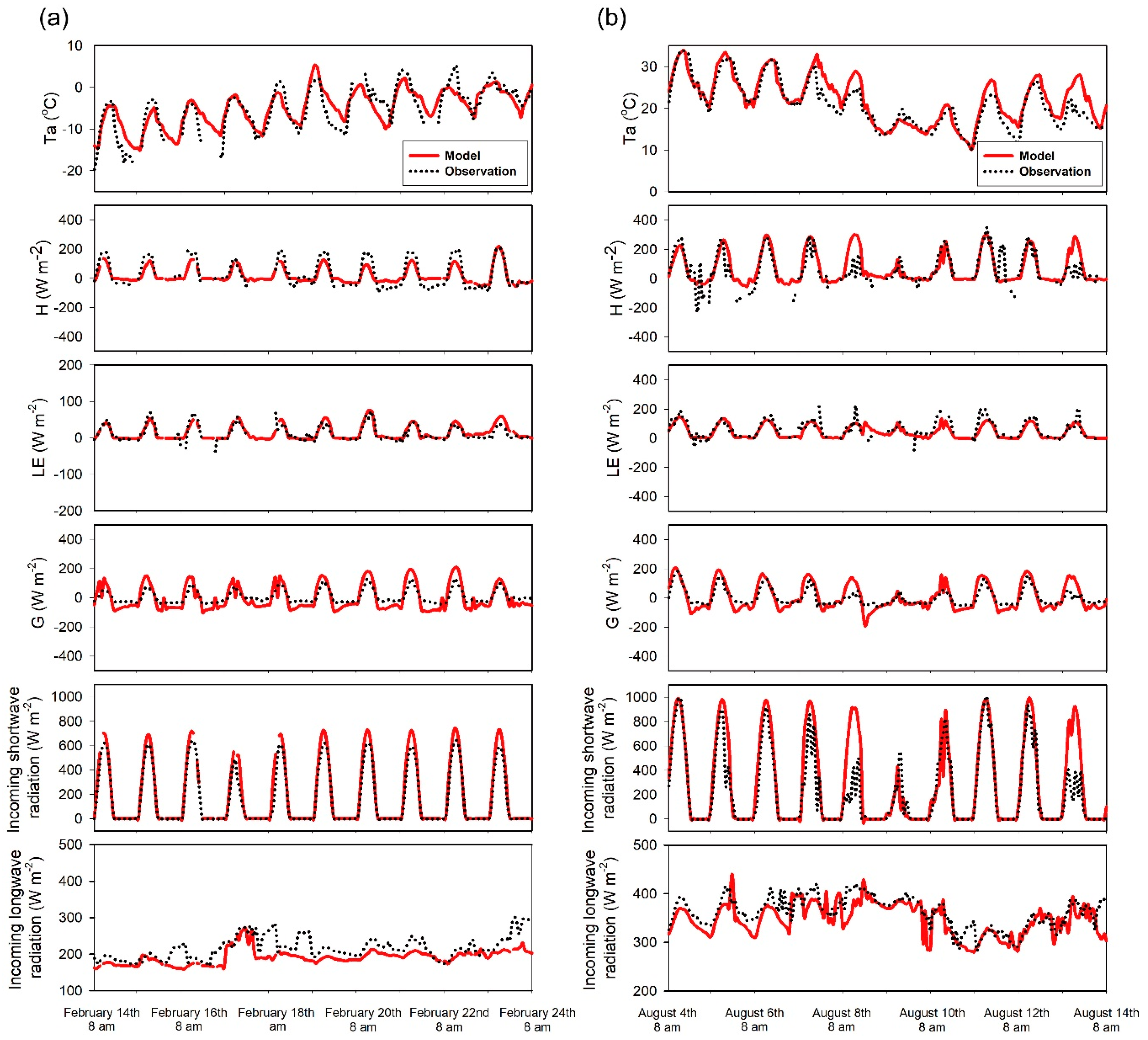
3.1. Model Evaluation
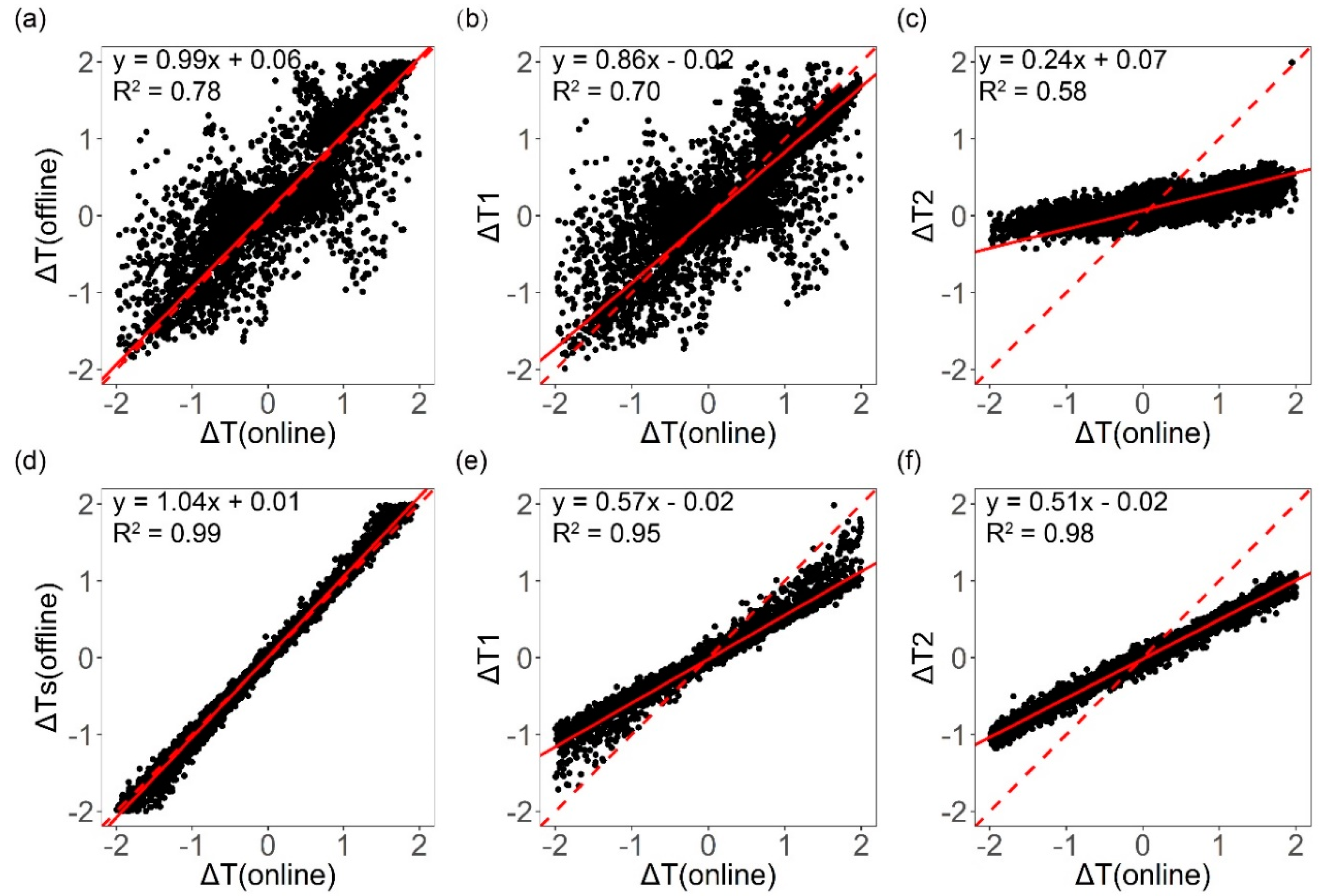
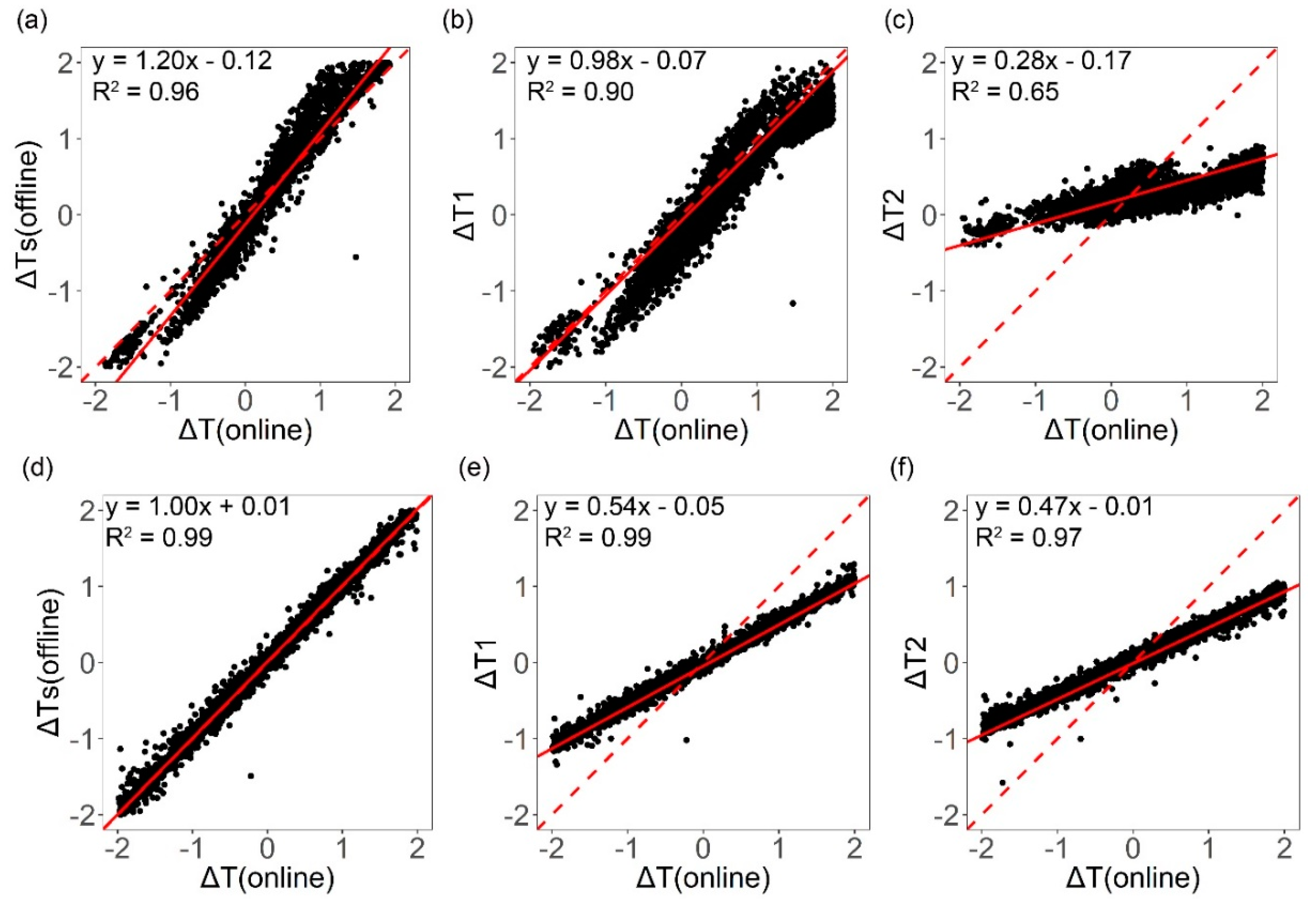
3.2. Online versus Offline Surface Temperature Change
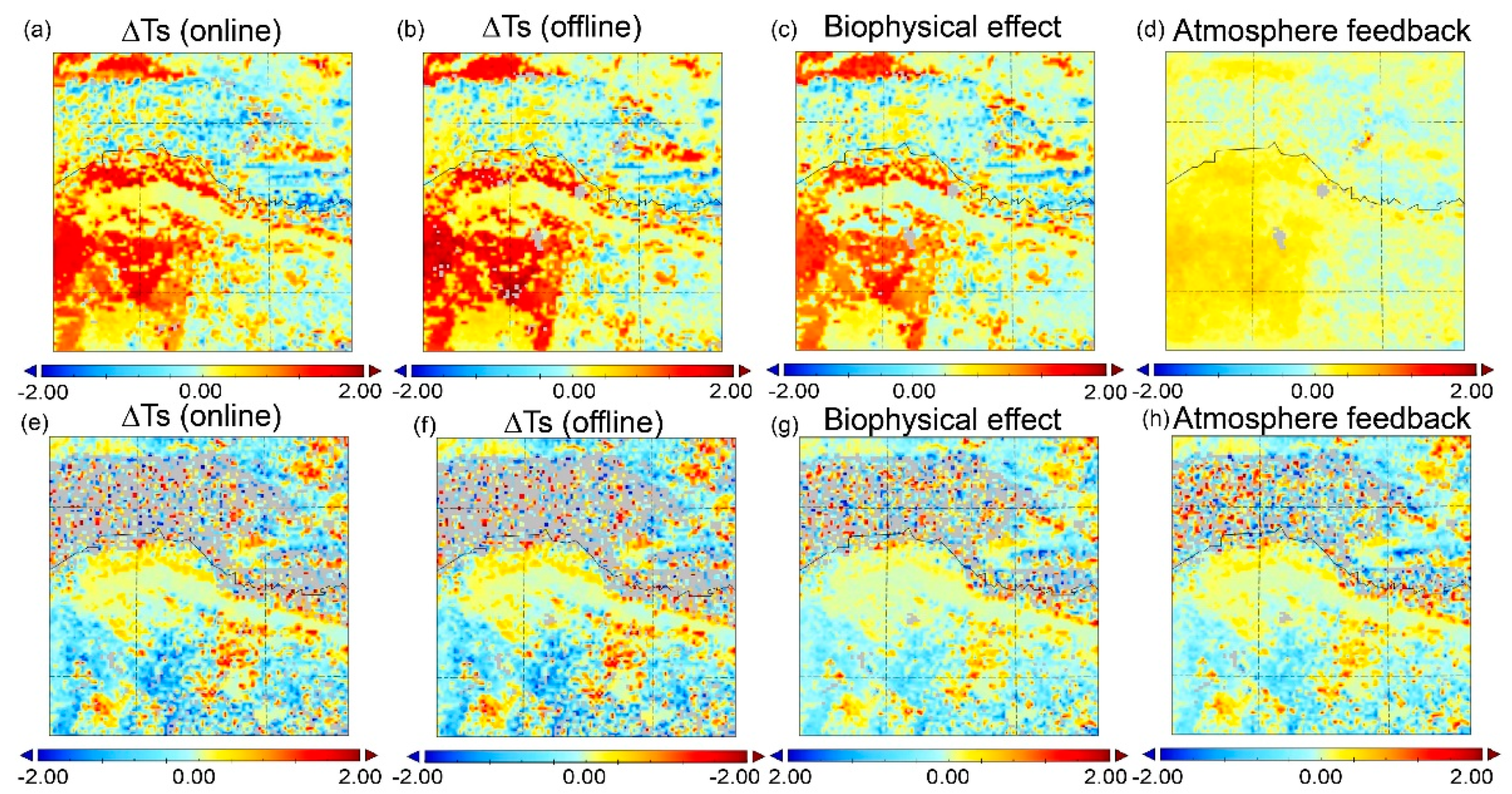
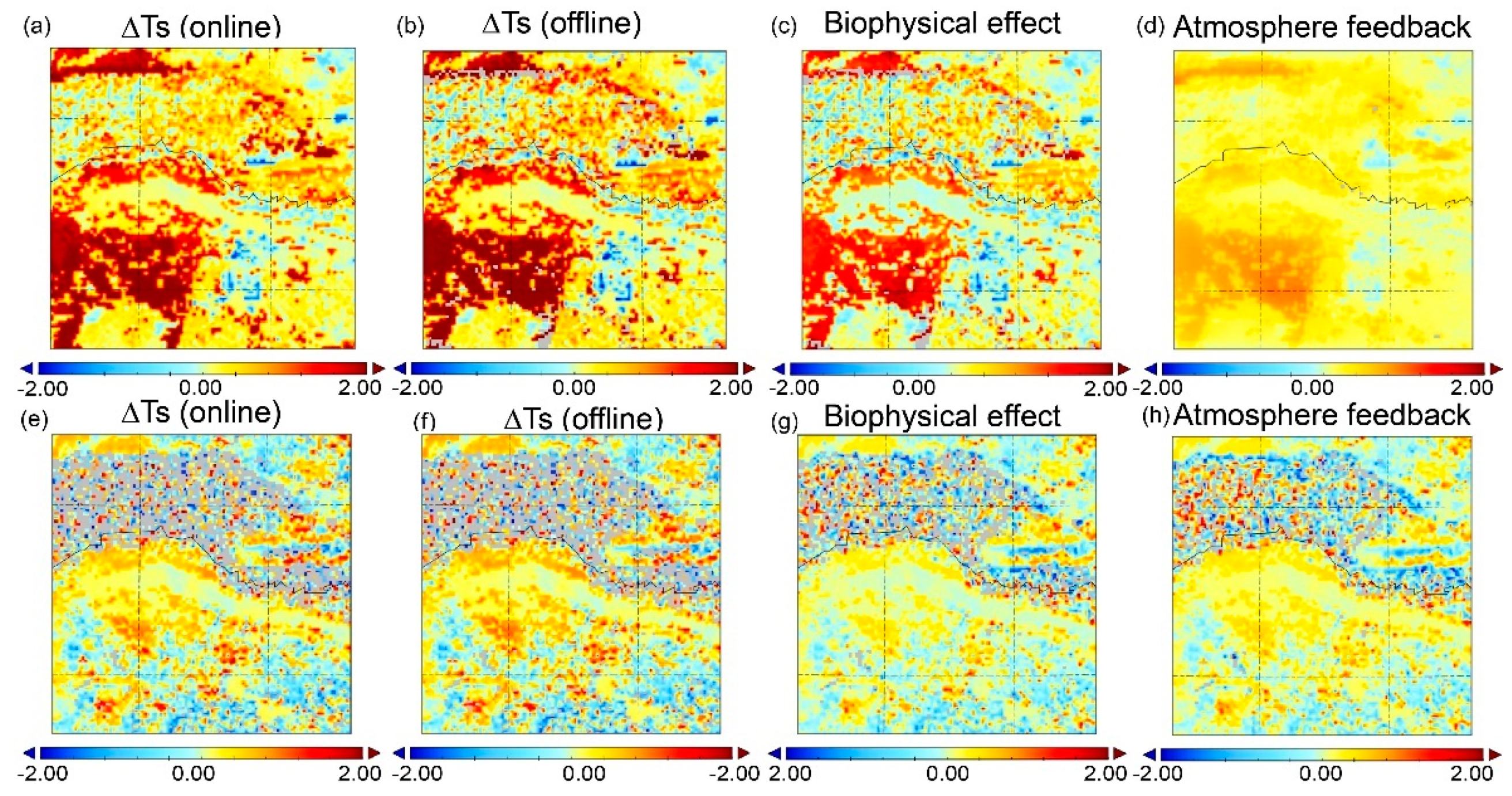
3.3. Seasonal Differences
3.4. Daytime versus Nighttime
4. Discussion
4.1. Warming Effect in the Daytime
4.2. Intrinsic Biophysical Effect versus Atmospheric Feedback
4.3. Limitations and Future Work
5. Conclusions
Supplementary Materials
Author Contributions
Funding
Acknowledgments
Conflicts of Interest
References
- FAO. Global Forest Resources Assessment 2010. FAO: Rome, 2010. Available online: http://www.fao.org/docrep/013/i1757e/i1757e.pdf (accessed on 25 March 2018).
- Caliskan, S.; Boydak, M. Afforestation of arid and semiarid ecosystems in Turkey. Turk. J. Agric. For. 2017, 41, 317–330. [Google Scholar] [CrossRef]
- Maestre, F.T.; Cortina, J. Are Pinus hatepensis plantations useful as a restoration tool in semiarid Mediterranean areas? For. Ecol. Manag. 2004, 198, 303–317. [Google Scholar] [CrossRef]
- Le Houerou, H.N. Restoration and rehabilitation of arid and semiarid Mediterranean ecosystems in North Africa and west Asia: A review. Arid Soil Res. Rehab. 2000, 14, 3–14. [Google Scholar] [CrossRef]
- State Forestry Administration of the People’s Republic of China. Eighth National Forest Resource Inventory Report (2009–2013). 2013. Available online: http://211.167.243.162:8085/8/chengguobaogao/showpageinit (accessed on 26 March 2018).
- Elion Resource Company of China. Personal communication, 2016.
- Li, W. Building Consensus Kubuqi International Desert Forum. China Today 2015, 9, 47–49. [Google Scholar]
- Charney, J.; Quirk, W.J.; Chow, S.H.; Kornfield, J. Comparative-Study of Effects of Albedo Change on Drought in Semi-Arid Regions. J. Atmos. Sci. 1977, 34, 1366–1385. [Google Scholar] [CrossRef]
- Snyder, P.K.; Delire, C.; Foley, J.A. Evaluating the influence of different vegetation biomes on the global climate. Clim. Dynam. 2004, 23, 279–302. [Google Scholar] [CrossRef]
- Bonan, G.B. Forests and climate change: Forcings, feedbacks, and the climate benefits of forests. Science 2008, 320, 1444–1449. [Google Scholar] [CrossRef]
- Bright; Zhao, K.G.; Jackson, R.B.; Cherubini, F. Quantifying surface albedo and other direct biogeophysical climate forcings of forestry activities. Glob. Chang. Biol. 2015, 21, 3246–3266. [Google Scholar] [CrossRef]
- Bala, G.; Caldeira, K.; Wickett, M.; Phillips, T.J.; Lobell, D.B.; Delire, C.; Mirin, A. Combined climate and carbon-cycle effects of large-scale deforestation. Proc. Natl. Acad. Sci. USA 2007, 104, 6550–6555. [Google Scholar] [CrossRef] [PubMed] [Green Version]
- Bright, R.M.; Anton-Fernandez, C.; Astrup, R.; Cherubini, F.; Kvalevag, M.; Stromman, A.H. Climate change implications of shifting forest management strategy in a boreal forest ecosystem of Norway. Glob. Chang. Biol. 2014, 20, 607–621. [Google Scholar] [CrossRef]
- Davin, E.L.; de Noblet-Ducoudre, N. Climatic Impact of Global-Scale Deforestation: Radiative versus Nonradiative Processes. J. Clim. 2010, 23, 97–112. [Google Scholar] [CrossRef]
- Mahmood, R.; Pielke, R.A.; Hubbard, K.G.; Niyogi, D.; Dirmeyer, P.A.; McAlpine, C.; Carleton, A.M.; Hale, R.; Gameda, S.; Beltran-Przekurat, A.; et al. Land cover changes and their biogeophysical effects on climate. Int. J. Climatol. 2014, 34, 929–953. [Google Scholar] [CrossRef]
- Feddema, J.J.; Oleson, K.W.; Bonan, G.B.; Mearns, L.O.; Buja, L.E.; Meehl, G.A.; Washington, W.M. The importance of land-cover change in simulating future climates. Science 2005, 310, 1674–1678. [Google Scholar] [CrossRef]
- Georgescu, M.; Lobell, D.B.; Field, C.B. Direct climate effects of perennial bioenergy crops in the United States. Proc. Natl. Acad. Sci. USA 2011, 108, 4307–4312. [Google Scholar] [CrossRef] [PubMed] [Green Version]
- Pielke, R.A.; Pitman, A.; Niyogi, D.; Mahmood, R.; McAlpine, C.; Hossain, F.; Goldewijk, K.K.; Nair, U.; Betts, R.; Fall, S.; et al. Land use/land cover changes and climate: Modeling analysis and observational evidence. Wires Clim. Chang. 2011, 2, 828–850. [Google Scholar] [CrossRef]
- Peng, S.S.; Piao, S.L.; Zeng, Z.Z.; Ciais, P.; Zhou, L.M.; Li, L.Z.X.; Myneni, R.B.; Yin, Y.; Zeng, H. Afforestation in China cools local land surface temperature. Proc. Natl. Acad. Sci. USA 2014, 111, 2915–2919. [Google Scholar] [CrossRef] [Green Version]
- Cao, Q.; Yu, D.Y.; Georgescu, M.; Han, Z.; Wu, J.G. Impacts of land use and land cover change on regional climate: A case study in the agro-pastoral transitional zone of China. Environ. Res. Lett. 2015, 10. [Google Scholar] [CrossRef]
- Skamarock, C.; Klemp, B.; Dudhia, J.; Gill, O.; Barker, D.; Duda, G.; Huang, X.; Wang, W.; Powers, G. A description of the Advanced Research WRF version 3. NCAR Tech. Note NCAR/TN-475+STR 2008, 113. [Google Scholar] [CrossRef]
- Ge, Q.S.; Zhang, X.Z.; Zheng, J.Y. Simulated effects of vegetation increase/decrease on temperature changes from 1982 to 2000 across the Eastern China. Int. J. Climatol. 2014, 34, 187–196. [Google Scholar] [CrossRef]
- Giorgi, F.; Marinucci, M.R.; Bates, G.T. Development of a 2nd-Generation Regional Climate Model (Regcm2). 1. Boundary-Layer and Radiative-Transfer Processes. Mon. Weather Rev. 1993, 121, 2794–2813. [Google Scholar] [CrossRef]
- Giorgi, F.; Marinucci, M.R.; Bates, G.T.; Decanio, G. Development of a 2nd-Generation Regional Climate Model (Regcm2). 2. Convective Processes and Assimilation of Lateral Boundary-Conditions. Mon. Weather Rev. 1993, 121, 2814–2832. [Google Scholar] [CrossRef]
- Liu, Y.Q.; Stanturf, J.; Lu, H.Q. Modeling the potential of the Northern China forest shelterbelt in improving hydroclimate conditions. J. Am. Water Resour. Assoc. 2008, 44, 1176–1192. [Google Scholar] [CrossRef]
- Zhang, X.F.; Adamowski, J.F.; Deo, R.C.; Xu, X.Y.; Zhu, G.F.; Cao, J.J. Effects of Afforestation on Soil Bulk Density and pH in the Loess Plateau, China. Water 2018, 10, 1710. [Google Scholar] [CrossRef]
- Kuriqi, A. Assessment and quantification of meteorological data for implementation of weather radar in mountainous regions. Mausam 2016, 67, 789–802. [Google Scholar]
- Lee, X.; Goulden, M.L.; Hollinger, D.Y.; Barr, A.; Black, T.A.; Bohrer, G.; Bracho, R.; Drake, B.; Goldstein, A.; Gu, L.; et al. Observed increase in local cooling effect of deforestation at higher latitudes. Nature 2011, 479, 384–387. [Google Scholar] [CrossRef] [Green Version]
- Zhao, L.; Lee, X.H.; Smith, R.B.; Oleson, K. Strong contributions of local background climate to urban heat islands. Nature 2014, 511, 216–219. [Google Scholar] [CrossRef]
- Chen, L.; Dirmeyer, P.A. Adapting observationally based metrics of biogeophysical feedbacks from land cover/land use change to climate modeling. Environ. Res. Lett. 2016, 11. [Google Scholar] [CrossRef]
- Schultz, N.M.; Lee, X.; Lawrence, P.J.; Lawrence, D.M.; Zhao, L. Assessing the use of subgrid land model output to study impacts of land cover change. J. Geophys. Res. Atmos. 2016, 121, 6133–6147. [Google Scholar] [CrossRef]
- Cess, R.D. Global Climate Change—Investigation of Atmospheric Feedback Mechanisms. Tellus 1975, 27, 193–198. [Google Scholar] [CrossRef]
- Cess, R.D.; Potter, G.L.; Blanchet, J.P.; Boer, G.J.; Ghan, S.J.; Kiehl, J.T.; H, L.E.T.; Li, Z.X.; Liang, X.Z.; Mitchell, J.F.; et al. Interpretation of cloud-climate feedback as produced by 14 atmospheric general circulation models. Science 1989, 245, 513–516. [Google Scholar] [CrossRef]
- Green, J.K.; Konings, A.G.; Alemohammad, S.H.; Berry, J.; Entekhabi, D.; Kolassa, J.; Lee, J.E.; Gentine, P. Regionally strong feedbacks between the atmosphere and terrestrial biosphere. Nat. Geosci. 2017, 10, 410–414. [Google Scholar] [CrossRef]
- He, Y.F.; D’Odorico, P.; De Wekker, S.F.J. The role of vegetation-microclimate feedback in promoting shrub encroachment in the northern Chihuahuan desert. Glob. Chang. Biol. 2015, 21, 2141–2154. [Google Scholar] [CrossRef]
- Wang, L.M.; Lee, X.H.; Schultz, N.; Chen, S.P.; Wei, Z.W.; Fu, C.S.; Gao, Y.Q.; Yang, Y.Z.; Lin, G.H. Response of Surface Temperature to Afforestation in the Kubuqi Desert, Inner Mongolia. J. Geophys. Res. Atmos. 2018, 123, 948–964. [Google Scholar] [CrossRef]
- Ek, M.B.; Mitchell, K.E.; Lin, Y.; Rogers, E.; Grunmann, P.; Koren, V.; Gayno, G.; Tarpley, J.D. Implementation of Noah land surface model advances in the National Centers for Environmental Prediction operational mesoscale Eta model. J. Geophys. Res. Atmos. 2003. [Google Scholar] [CrossRef]
- Tewari, M.; Chen, F.; Wang, W.; Dudhia, J.; LeMone, M.; Mitchell, K.; Ek, M.; Gayno, G.; Wegiel, J.; Cuenca, R. Implementation and verification of the unified NOAH land surface model in the WRF model. In Proceedings of 20th Conference on Weather Analysis and Forecasting/16th Conference on Numerical Weather Prediction; American Meteorological Society: Seattle, WA, USA, 2004; Volume 1115. [Google Scholar]
- Grell, G.A.; Freitas, S.R. A scale and aerosol aware stochastic convective parameterization for weather and air quality modeling. Atmos. Chem. Phys. 2014, 14, 5233–5250. [Google Scholar] [CrossRef] [Green Version]
- Monin, A.S.; Obukhov, A.M. Basic laws of turbulent mixing in the surface layer of the atmosphere. Contrib. Geophys. Inst. Acad. Sci. USSR 1954, 151, e187. [Google Scholar]
- Janić, Z.I. Nonsingular Implementation of the Mellor-Yamada Level 2.5 Scheme in the NCEP Meso Model; Office Note No. 437; National Centers for Environmental Prediction: Washington, DC, USA, 2011; p. 61. [Google Scholar]
- Collins, W.D.; Rasch, P.J.; Boville, B.A.; Hack, J.J.; McCaa, J.R.; Williamson, D.L.; Briegleb, B.P.; Bitz, C.M.; Lin, S.J.; Zhang, M.H. The formulation and atmospheric simulation of the Community Atmosphere Model version 3 (CAM3). J. Clim. 2006, 19, 2144–2161. [Google Scholar] [CrossRef]
- Collins, W.D.; Rasch, P.J.; Boville, B.A.; Hack, J.J.; McCaa, J.R.; Williamson, D.L.; Kiehl, J.T.; Briegleb, B.; Bitz, C.; Lin, S.J. Description of the NCAR community atmosphere model (CAM 3.0). NCAR Tech. Note NCAR/TN-464+ STR 2004, 226, 4–9. [Google Scholar]
- Hong, S.Y.; Dudhia, J.; Chen, S.H. A revised approach to ice microphysical processes for the bulk parameterization of clouds and precipitation. Mon. Weather Rev. 2004, 132, 103–120. [Google Scholar] [CrossRef]
- Noh, Y.; Cheon, W.G.; Hong, S.Y.; Raasch, S. Improvement of the K-profile model for the planetary boundary layer based on large eddy simulation data. Bound-Lay. Meteorol. 2003, 107, 401–427. [Google Scholar] [CrossRef]
- Hong, S.Y.; Noh, Y.; Dudhia, J. A new vertical diffusion package with an explicit treatment of entrainment processes. Mon. Weather Rev. 2006, 134, 2318–2341. [Google Scholar] [CrossRef]
- Eskridge, R.E.; Ku, J.Y.; Rao, S.T.; Porter, P.S.; Zurbenko, I.G. Separating different scales of motion in time series of meteorological variables. Bull. Am. Meteorol. Soc. 1997, 78, 1473–1483. [Google Scholar] [CrossRef]
- Zhao, Y.Y.; Feng, D.L.; Yu, L.; Wang, X.Y.; Chen, Y.L.; Bai, Y.Q.; Hernandez, H.J.; Galleguillos, M.; Estades, C.; Biging, G.S.; et al. Detailed dynamic land cover mapping of Chile: Accuracy improvement by integrating multi-temporal data. Remote Sens. Environ. 2016, 183, 170–185. [Google Scholar] [CrossRef]
- Feng, D.L.; Zhao, Y.Y.; Yu, L.; Li, C.C.; Wang, J.; Clinton, N.; Bai, Y.Q.; Belward, A.; Zhu, Z.L.; Gong, P. Circa 2014 African land-cover maps compatible with FROM-GLC and GLC2000 classification schemes based on multi-seasonal Landsat data. Int. J. Remote Sens. 2016, 37, 4648–4664. [Google Scholar] [CrossRef]
- Chinese Meteorological Administration. Specifications for Surface Meteorological Observation; China Meteorological Press: Beijing, China, 2003.
- Schultz, N.M.; Lawrence, P.J.; Lee, X. Global satellite data highlights the diurnal asymmetry of the surface temperature response to deforestation. J. Geophys. Res. Biogeosci. 2017, 122. [Google Scholar] [CrossRef]
- Zhang, Q.; Pan, Y.; Wang, S.; Xu, J.; Tang, J. High-Resolution Regional Reanalysis in China: Evaluation of 1 Year Period Experiments. J. Geophys. Res. Atmos. 2017, 122. [Google Scholar] [CrossRef]
- Abera, T.A.; Heiskanen, J.; Pellikka, P.; Rautiainen, M.; Maeda, E.E. Clarifying the role of radiative mechanisms in the spatio-temporal changes of land surface temperature across the Horn of Africa. Remote Sens. Environ. 2019, 221, 210–224. [Google Scholar] [CrossRef]
- Rotenberg, E.; Yakir, D. Distinct patterns of changes in surface energy budget associated with forestation in the semiarid region. Glob. Chang. Biol. 2011, 17, 1536–1548. [Google Scholar] [CrossRef]


| Items | Description |
|---|---|
| Model version | WRF 3.7.1 |
| Dynamics solver | Advanced Research WRF |
| Time step | 30 s |
| Output interval | 1 h |
| Vertical level | 27 |
| Radiation scheme | CAM3 a |
| Surface model | Noah land surface model [37,38] |
| Cumulus scheme | Grell-Freitas ensemble scheme [39] |
| Microphysic scheme | WSM3 b |
| PBL scheme | YSU c |
| Surface layer | Monin-Obukhov [40,41] |
| Land Change Type | Area (km2) | Time | ΔK↓ | ΔL↓ | ΔTa | ΔT1 | ΔT2 | Albedo Term1 | Roughness Term2 | Bowen Ratio Term3 | Soil Heat Flux Term4 | K↓ Term5 | L↓ Term6 | Ta Term7 | Sum (Terms 1 through 7) |
|---|---|---|---|---|---|---|---|---|---|---|---|---|---|---|---|
| No change | 30,552 | winter daytime | −0.11 | 0.34 | 0.17 | 0.02 | 0.18 | 0.02 | 0.02 | −0.02 | 0.00 | 0.00 | 0.01 | 0.17 | 0.20 |
| winter nighttime | 0.00 | 0.11 | 0.00 | −0.01 | 0 | 0.00 | −0.02 | 0 | 0.01 | 0.00 | 0.00 | 0.00 | −0.01 | ||
| summer daytime | −0.84 | 0.50 | 0.07 | −0.03 | 0.07 | 0.01 | 0.04 | −0.05 | −0.03 | −0.01 | 0.01 | 0.07 | 0.04 | ||
| summer nighttime | 0.00 | −0.28 | −0.13 | −0.06 | −0.06 | 0.00 | −0.06 | −0.02 | 0.02 | 0.00 | 0.00 | −0.06 | −0.12 | ||
| Bare land to shrub | 10,268 | winter daytime | −3.49 | 2.56 | 0.63 | 1.51 | 0.58 | 1.11 | −0.05 | 0.37 | 0.08 | −0.05 | 0.06 | 0.57 | 2.09 |
| winter nighttime | 0.00 | 0.92 | 0.04 | 0.12 | 0.1 | 0.00 | 0.07 | 0.01 | 0.04 | 0.00 | 0.01 | 0.09 | 0.22 | ||
| summer daytime | −9.31 | 6.83 | 0.33 | 0.97 | 0.37 | 1.74 | −0.44 | −0.16 | −0.17 | −0.14 | 0.18 | 0.33 | 1.34 | ||
| summer nighttime | 0.00 | 2.02 | −0.39 | −0.26 | −0.22 | 0.00 | −0.37 | 0.01 | 0.10 | 0.00 | 0.02 | −0.24 | −0.48 | ||
| Shrub to grass | 2332 | winter daytime | −1.97 | 1.62 | 0.35 | 0.68 | 0.31 | 0.77 | −0.28 | 0.19 | 0.00 | −0.04 | 0.05 | 0.30 | 0.99 |
| winter nighttime | 0.00 | 0.86 | 0.05 | −0.02 | −0.01 | 0.00 | −0.06 | 0.01 | 0.03 | 0.00 | 0.04 | −0.05 | −0.03 | ||
| summer daytime | −4.69 | 1.95 | 0.00 | −0.44 | 0 | 0.87 | −0.13 | −0.97 | −0.21 | −0.09 | 0.05 | 0.04 | −0.44 | ||
| summer nighttime | 0.00 | 1.34 | −0.48 | −0.16 | −0.19 | 0.00 | −0.25 | −0.14 | 0.23 | 0.00 | 0.04 | −0.23 | −0.35 | ||
| Cropland to grass | 992 | winter daytime | 0.29 | −0.58 | 0.13 | 0.03 | 0.12 | −0.14 | 0.20 | −0.02 | −0.01 | 0.01 | −0.02 | 0.13 | 0.15 |
| winter nighttime | 0.00 | −0.64 | −0.01 | −0.13 | −0.07 | 0.00 | −0.17 | 0.01 | 0.03 | 0.00 | −0.03 | −0.04 | −0.20 | ||
| summer daytime | 0.33 | −2.67 | 0.01 | 0.13 | −0.02 | −0.24 | 0.24 | 0.11 | 0.02 | 0.01 | −0.06 | 0.03 | 0.11 | ||
| summer nighttime | 0.00 | −2.81 | −0.16 | −0.06 | −0.19 | 0.00 | −0.06 | −0.01 | 0.01 | 0.00 | −0.09 | −0.10 | −0.25 | ||
| Shrub to cropland | 644 | winter daytime | −2.53 | 1.78 | 0.32 | 0.59 | 0.27 | 0.88 | −0.58 | 0.23 | 0.06 | −0.04 | 0.05 | 0.26 | 0.86 |
| winter nighttime | 0.00 | 1.39 | 0.24 | 0.22 | 0.25 | 0.00 | 0.25 | 0.01 | −0.04 | 0.00 | 0.04 | 0.21 | 0.47 | ||
| summer daytime | −5.83 | 4.34 | −0.01 | −0.69 | −0.01 | 0.95 | −0.52 | −1.02 | −0.10 | −0.09 | 0.09 | −0.01 | −0.7 | ||
| summer nighttime | 0.00 | 4.39 | −0.36 | −0.24 | −0.10 | 0.00 | −0.39 | −0.06 | 0.21 | 0.00 | 0.09 | −0.19 | −0.34 | ||
| Whole domain | 46,648 | winter daytime | −0.95 | 0.86 | 0.29 | 0.38 | 0.29 | 0.30 | −0.02 | 0.08 | 0.02 | −0.01 | 0.02 | 0.28 | 0.67 |
| winter nighttime | 0.00 | 0.30 | 0.03 | 0.03 | 0.03 | 0.00 | 0.01 | 0.00 | 0.02 | 0.00 | 0.01 | 0.02 | 0.06 | ||
| summer daytime | −2.88 | 1.91 | 0.12 | 0.01 | 0.14 | 0.28 | −0.08 | −0.12 | −0.07 | −0.04 | 0.05 | 0.13 | 0.15 | ||
| summer nighttime | 0.00 | 0.28 | −0.11 | −0.1 | −0.1 | 0.00 | −0.12 | −0.02 | 0.04 | 0.00 | 0.00 | −0.10 | −0.2 |
© 2019 by the authors. Licensee MDPI, Basel, Switzerland. This article is an open access article distributed under the terms and conditions of the Creative Commons Attribution (CC BY) license (http://creativecommons.org/licenses/by/4.0/).
Share and Cite
Wang, L.; Lee, X.; Feng, D.; Fu, C.; Wei, Z.; Yang, Y.; Yin, Y.; Luo, Y.; Lin, G. Impact of Large-Scale Afforestation on Surface Temperature: A Case Study in the Kubuqi Desert, Inner Mongolia Based on the WRF Model. Forests 2019, 10, 368. https://0-doi-org.brum.beds.ac.uk/10.3390/f10050368
Wang L, Lee X, Feng D, Fu C, Wei Z, Yang Y, Yin Y, Luo Y, Lin G. Impact of Large-Scale Afforestation on Surface Temperature: A Case Study in the Kubuqi Desert, Inner Mongolia Based on the WRF Model. Forests. 2019; 10(5):368. https://0-doi-org.brum.beds.ac.uk/10.3390/f10050368
Chicago/Turabian StyleWang, Liming, Xuhui Lee, Duole Feng, Congsheng Fu, Zhongwang Wei, Yanzheng Yang, Yizhou Yin, Yong Luo, and Guanghui Lin. 2019. "Impact of Large-Scale Afforestation on Surface Temperature: A Case Study in the Kubuqi Desert, Inner Mongolia Based on the WRF Model" Forests 10, no. 5: 368. https://0-doi-org.brum.beds.ac.uk/10.3390/f10050368