Interregional Crown Width Models for Individual Trees Growing in Pure and Mixed Stands in Austria

Abstract

Crown width is a functional trait that is commonly used to improve the estimation of above-ground biomass of forests and is often included as a predictor variable in forest growth models. Most of the existing crown width models reflect the relationship between crown width, tree size and competition variables, but do not consider the effect of species mixture. In this study, we developed crown width models for individual-tree of the major tree species growing in Austria. Because these models should be applicable for mixed and pure stands and should also take into account the characteristics of different sites, the relationship between crown width, site variables and species composition was investigated. For that purpose, we used data from a sub-sample of the Austrian National Forest Inventory, which comprises crown width measurements of about 8900 trees from 1508 sample plots. Because of the hierarchical structure of the data set (i.e., trees nested within the plot) which destroys the independencies between observations, linear mixed-effects models were used. The species composition of the stand was included via the species-specific relative proportions of basal area. To describe the interregional variability of crown width, dummy variables were introduced, which account for region-specific differences. Site characteristics were incorporated through the altitude, slope and aspect of the site. For Norway spruce, silver fir, Scots pine, European larch, European beech, oak species and ash/maple species it was possible to develop crown width models, which reflect the effects of site characteristics and species composition of the stand. The crown widths of shade-tolerant species reacted mainly positively to admixture, whereas light-demanding species reacted with decreasing crown widths. Coniferous species were not as strongly affected by mixture as broadleaf species.

1. Introduction

Tree crown dimensions are important functional traits, which are commonly incorporated in growth models used as decision-support tools in forest management [1,2,3,4]. Crown size is considered to be an indirect measure of the photosynthetic capacity of a tree and is strongly correlated to tree growth [5,6]. Usually, crown size is described by crown length, crown ratio and/or crown width (CW). The analysis of these variables is important for quantifying and qualifying growth stage, tree vigor and stability [7]. CW is often used as a predictor variable in increment models [8], biomass equations [9,10] and as a component in competition indices [11]. CW can also be used for the estimation and simulation of crown and canopy cover [12,13] and light interception in the canopy [14]. Despite the numerous application possibilities of CW, it is costly and time consuming to measure the CW of trees. Therefore, accurate models based on adequate numbers of observations are required to predict the crown width of trees. Most of the existing CW models are simple linear or non-linear functions of diameter at breast height (DBH) and other tree size variables, estimated using ordinary least squares techniques [13,15], or mixed-effects models [16,17]. The more detailed CW models also consider the site and stand characteristics like site index, the elevation of the site, stand density or the competitive situation of the observed trees, which have a significantly high influence on the crown dimensions [18,19].

There is widespread and general agreement that the ability of trees to plastically adapt the shape and size of their crowns to their local competitive environment allows mixed-species forests to optimize the use of canopy space. The so-called canopy packing efficiency was found to be higher in species-rich forests and trees in mixed forests can have larger crowns than those in monocultures [20,21]. The leaf area distribution of Norway spruce and European larch is also effected by mixture [22] and species composition affects the crown structure of European beech [23]. Although the effect of species composition on the crown dimensions was already described in several studies, only a few CW models exist, which incorporate the species composition and distinguish between pure and mixed forests [21,24,25]. CW models for Austrian forests, which are applicable for both mixed and pure forest stands, have not been developed so far. However, crown width measurements are available from the Austrian National Forest Inventory (ANFI). Augmented with descriptive information about the sites and stand characteristics, these measurements build a huge and unique database to investigate the effect of species mixture on the crown dimensions. Furthermore, these measurements allow us to develop CW models, which are planned to be implemented in the Austrian forest growth simulator CALDIS-VB V0.1 [26], which is an individual-tree based, distance-independent and climate-sensitive growth simulator of the FVS-type (Forest Vegetation Simulator) [1,2,3,4] developed at the federal research centre for forests (BFW) in Vienna, Austria. It consists of a basal area increment model, a height increment model, an ingrowth model and a model describing salvage cuts and tree mortality. All these sub-models were calibrated with data from the ANFI. CALDIS-VB V0.1 was successfully applied in a recent study about greenhouse gas dynamics in forests [27], which required a solid estimation of the above-ground biomass, particularly branch and needle mass. In order to improve the biomass estimation, the main objective of our research was to develop individual-tree based CW models for the most important tree species growing in Austria, which take the effects of species mixture into account.

2. Materials and Methods

To enable the development of crown width models for the major tree species in Austria, several thousands tree crowns were measured within the last re-assessment period of the ANFI. Beside the radii of the crowns, many other traits of the trees, stands and sites were assessed. All traits, which are important for our stdy, are summerised in

Table 1. List of variables, their abbreviations, and definitions.

Abbreviation	Variable/Definition	Unit
CW	Crown width	m
DBH	Diameter at breast height (1.3 m)	cm
H	Height of a tree	m
HCB	Height of a trees’s crown base	m
CR	Crown ratio = 1 − HCB/H
H/D	Height − diameter ratio = H [cm]/DBH [cm]
ELEV	Sea level of the sample plot	hectometre
EXP	Azimuth of the aspect of the sample area	radiant
SL	Slope gradient of the sample area	percentage
Region_x	Growth region [28] in which the sample plot is located
PS_x	Relative proportion of basal area of species x (x … species code)
PSL_x	Relative proportion of basal area of species x (x … species code) considering only trees of the same crown layer

.

2.1. Material

The last full ANFI assessment has been run from 2007 to 2009. During this inventory measurements of crown radii in four directions were taken from the trees of a sub-sample of the inventory plots. The approximately 22,000 sample plots of the ANFI cover on a 3.89 × 3.89 km sampling grid the whole Austrian territory, whereby about 50% of these plots are on forest area. These plots are clustered to tracts, each of which comprises four plots arranged in a square of 200 m × 200 m. To avoid that the treatment on the sample plots is different than outside the plot, a hidden plot design was used. Each sample plot consists of two concentric circles with fixed radii of 9.77 and 2.6 m and one angle count sample plot [29] using a basal area factor of 4 m²/ha. Site information, such as soil type, aspect, and slope were measured on the fixed plot with 9.77 m radius. Individual-tree data were collected via the smaller fixed plot for trees with a DBH between 5.0 and 10.4 cm and via angle count sampling for trees with a DBH larger than 10.4 cm. Tree species, DBH, tree height (H) and height of the crown base (HCB) were recorded for all sample trees. Measurements of tree crown radii were limited to a sub-sample which comprises only trees with DBH larger than 10.4 cm from one angle count sample plot of a tract. Crown radii were measured in four directions by plumbing the maximum extension of the tree’s crown in the respective direction. Crown width (CW) was calculated by doubling the quadratic mean of the 4 measurement values per tree. The species composition of each sample plot was described by the species-specific relative proportions of basal area (PS). The relative proportions of species were also calculated considering if trees were in the same crown layer as the observed tree (PSL) using the definition of crown layers according to Pretzsch [30]. In total, around 8900 tree crowns were measured at 1508 sample plots, whereby the larger part of the observations is for Norway spruce (Picea abies) with 5436 observations, and for European beech (Fagus sylvatica) with 811 observations (

Table 2. Summary statistics for model fitting data.

Species	Code	N	DBH in cm			H in m			CW in m
			Min	Mean	Max	Min	Mean	Max	Min	Mean	Max
Picea Abies Norway spruce	1	5436	10.5	34.8	115.3	4.8	24.5	53.3	1.2	5.6	16.4
Abies Alba Silver fir	2	272	10.7	40.5	89.0	7.3	27.5	43.0	2.6	6.9	13.9
Larix deciduas European larch	3	627	10.9	42.5	92.9	8.1	27.2	42.7	1.5	7.5	16.6
Pinus Sylvestris Scots pine	4	612	10.6	33.6	68.5	6.0	23.6	38.6	1.3	5.4	10.9
Pinus Nigra Austrian pine	5	97	11.3	37.0	79.6	6.6	18.5	34.3	2.0	5.9	12.1
Pinus Cembra Stone pine	6	48	19.4	42.4	80.0	9.0	16.5	30.3	2.6	5.7	8.7
Pinus strobus Weymouth pine	7	3	34.2	36.5	37.6	24.0	26.2	28.6	5.4	6.3	6.8
Pseudotsuga Menziesii Douglas fir	8	5	18.4	36.8	70.8	12.6	22.4	42.1	4.6	6.6	9.2
Fagus Sylvatica European beech	10	811	10.7	35.3	106.7	6.1	23.8	39.9	2.2	9.3	22.4
Quercus sp. Oak	11	238	10.7	36.3	90.3	8.7	21.3	36.8	2.1	8.1	21.0
Carpinus betulus Hornbeam	12	68	11.1	23.1	65.1	10.8	17.1	33.3	0.2	7.7	19.4
Fraxinus sp. Ash	13	192	10.9	28.3	71.7	6.9	23.5	38.8	1.8	7.0	20.5
Acer sp. Maple	14	96	11.4	29.7	110.4	8.8	20.0	32.3	3.0	7.8	19.7
Ulmus sp. Elm	15	8	13.3	36.2	60.8	13.5	21.5	32.0	6.7	9.5	16.3
Castanea sativa Spanish chestnut	16	15	10.5	25.8	51.5	11.1	17.5	25.5	4.3	6.6	10.7
Robinia pseudoacacia Robinia	17	27	10.6	20.0	37.6	9.6	17.7	29.8	2.4	5.5	10.4
Sorbus sp., Prunus sp.	18	26	10.7	22.1	48.7	6.5	15.2	25.9	1.6	6.2	13.2
Betula sp. Birch	20	86	10.5	26.2	52.2	8.8	19.1	33.0	2.0	5.7	11.2
Alnus glutinosa Black alder	21	94	11.4	26.0	46.1	9.9	21.7	29.9	2.3	5.7	10.9
Alnus incana White alder	22	25	11.3	17.7	30.9	9.0	13.8	24.9	0.1	3.7	7.1
Tilia sp.	23	29	11.6	28.5	79.9	10.4	19.1	34.3	3.6	7.3	18.3
Populus tremula, Populus Alba Trembling and white poplar	24	22	11.1	29.9	67.9	11.2	19.8	31.0	3.3	7.2	14.3
Populus Nigra Black poplar	25	8	25.5	47.9	77.5	17.9	26.1	32.4	3.8	9.2	15.1
Populus sp. X Hybrid poplar	26	15	17.7	46.9	86.2	14.8	23.7	31.5	3.8	8.9	12.9
Salix sp. Willow	27	22	12.8	24.3	56.5	7.8	13.1	30.3	5.9	7.9	12.5

).

2.2. Statistical Analysis

In our modeling approach we assumed that the CW of individual trees can be expressed as a function of four groups of variables: (1) site characteristics, (2) stand characteristics, and (3) tree size (Equation (1)).

$$CW=f \left(Site,Stand,Size\right).$$

(1)

However, measurements of CW and other parameters were available from trees growing on sample plots that are located in different stands and environments. This causes a hierarchical structure of the data (i.e., trees nested within the plot) which destroys the independencies between observations. Thus, linear mixed-effect models were used to analyze the trees’ crown width depending on various regressor variables. The mixed-effects model framework takes into account both the fixed effects of covariates and random effects. Fixed effects parameters are common to all subjects and random-effect parameters are specific to each subject [31]. Due to the complexity of the fixed effects structure and ensuing converging problems, only random intercept models were calibrated. All models were fitted with the restricted maximum likelihood (REML) techniques implemented in the R package “lme4” and provided by the function “lmer” [32]. Fixed effect parameters were tested using Wald tests implemented in the R-package “lmerTest” [33]. This package uses Satterthwaite’s method for approximating the degrees of freedom for the t- and F-tests, and overloads the summary function by attaching the p-values in order to test them. We used the following linear or log-linear function to model the CW of individual trees:

$$C{W}_{ij}=\alpha +{\displaystyle \sum }_{k=1}^l{a}_k{S}_{kj}+{\displaystyle \sum }_{m=1}^n{b}_m{X}_{mij}+u_j+{\epsilon }_{ij}$$

(2)

$$\ln (C{W}_{ij})=\alpha +{\displaystyle \sum }_{k=1}^l{a}_k{S}_{kj}+{\displaystyle \sum }_{m=1}^n{b}_m{X}_{mij}+u_j+{\epsilon }_{ij},$$

(3)

where $C{W}_{ij}$ is the crown width for tree $i$ on sample plot $j$, $\alpha$ is the population intercept, ${\displaystyle \sum }_{k=1}^l{a}_k{S}_{kj}$ and ${\displaystyle \sum }_{m=1}^n{b}_m{X}_{mij}$ are the fixed effects at plot and tree-level including the coefficients $a_k$ and the independent variables $S_{kj}$ for plot $j$ and the coefficients $b_m$ and the independent variables $X_{mij}$ for tree $i$ on sample plot $j$, $u_j$ is the random effect for the intercept with $u_j~N\left(0,\tau \right)$, and ${\epsilon }_{ij}$ is the residual error with ${\epsilon }_{ij}~N\left(0,\sigma \right)$. The independent variables $S_k$ and $X_m$ were taken from the three variable groups (cf. Equation (1)) comprising site (ELEV, EXP, SL, Region_x) and stand characteristics (PS_X or PSL_x) and tree size (DBH, H, CR, H/D). The full list of variables including their abbreviations and definitions is given in Table 1.

The modeling process was started with the incorporation of the tree size variables DBH and H. In the next step CR and H/D were added to the model. These two variables are strongly influenced by stand density and competition [16,24,34,35], and the actual CR and H/D are the result of a tree’s competitive situation in the past. After the tree-level variables were included in the model, site variables such as elevation (ELEV), slope (SL) and aspect (EXP) were tested whether they could help to explain the variation in CW. SL and EXP were incorporated in the model via the slope-aspect transformation of Stage [36], which is an interaction-term between SL and the sine and the cosine, respectively, of the azimuth of the aspect. The next step was to test if the addition of the species’ proportion improved the model. For that purpose, one model version was parameterized including PS_x and their interactions with ELEV. In the second version, PSL_x was used instead of PS_x also including interactions with ELEV. Then, these two versions were compared and assessed which version showed both better model fit statistics (Akaike Information Criterion—AIC, conditional and marginal Pseudo-R²) and a more plausible model behavior. By using PSL_x in the model it should be considered that small trees in lower crown layers do not have a competitive effect on the trees in higher crown layers, for example, fir regeneration under an old pine stand.

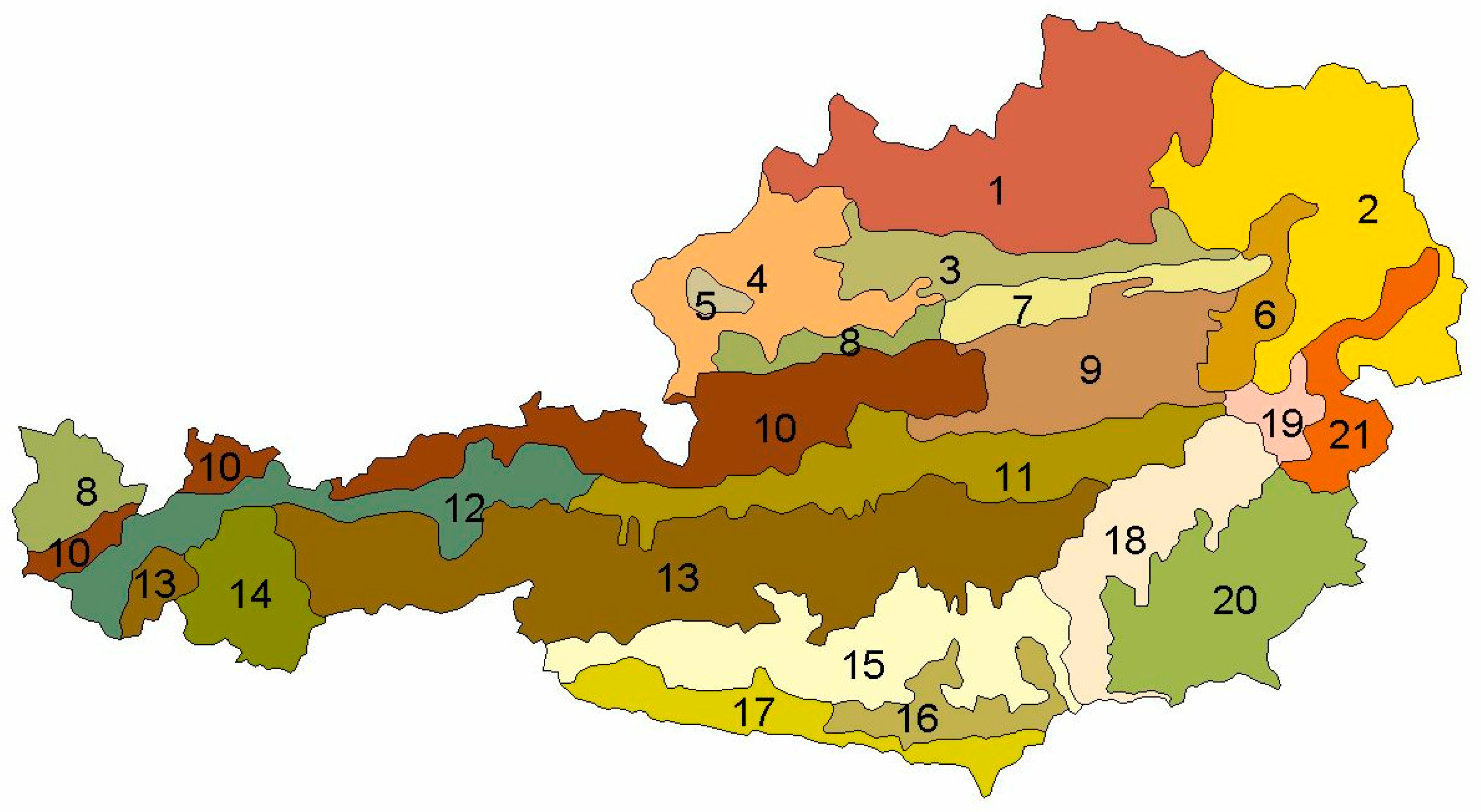
Austria is characterized by very contrasting landscapes reaching from high elevation sites in the Alps to the Pannonian basin in the eastern part of the country. For this reason, Jelem and Kilian [28] defined 21 different growth regions comprising areas with relatively similar growth conditions (Appendix A Figure A1). In order to capture a possible interregional variation in the DBH-CW relationship, dummy variables (Region_x) for these growth regions were included in the model and tested for effects on the intercept and the DBH variable.

The process of variable selection and model building was done separately for each tree species. However, for those species that had a too low number of observations to parameterize complex and meaningful CW models (n < 100), generic linear mixed-effects models were developed: one for coniferous and one for broadleaf species. In the generic models, dummy variables affecting the intercept and the DBH variable were used to consider differences between the various species.

Independent variables were only selected for the final model if their coefficients were significantly ($\alpha =0.05$) different from 0. The variance of the residuals was examined for homogeneity by means of residual plots. The decision to use the linear or the log-linear function for the final model (Equations (2) or (3)) was based on the model behavior, the model fit, and the homogeneity of the residual variance.

3. Results

3.1. Crown Width Models for Conifer Species

For Norway spruce (Picea abies), Silver fir (Abies alba), European larch (Larix decidua), and Scots pine (Pinus sylvestris) it was possible to build CW models that consider site and stand characteristics. For Austrian pine (Pinus nigra), stone pine (Pinus cembra), douglas fir (Pseudotsuga menziesii), and eastern white pine (Pinus strobus) the data were merged and a generic model was developed that did not include stand characteristics. The resulting parameter estimates can be seen in

Table 3. Parameter estimates of the mixed-effects crown width (CW)-models for conifer species. The dependent variable CW and diameter at breast height (DBH) of the CW-model for Scots pine were not transformed. All shown estimates were significant (p-values < 0.05), except values printed in italics.

Tree Species	Picea abies	Larix decidua	Pinus sylvestris	Abies alba	Other sp.
Depend Variable	ln(CW)	ln(CW)	CW	ln(CW)	ln(CW)
Intercept	0.052386	−0.4307885	3.7155099	1.4180761	−0.8317729
Region_4	-	-	-	−0.9031416	-
Region_6	−0.4215087	-	-	-	-
Region_13	-	0.0482368	-	-	-
Region_15	-	-	-	-	1.7352668
Region_11/12/15/18	0.046185	-	-	-	-
DBH	-	-	0.0898499	-	-
Region_19 * DBH	-	-	0.0194008	-	-
Region_20 * DBH	-	-	0.0130925	-	-
ln (DBH)	0.486831	0.6384635	-	0.4629727	0.8211466
Region_4 * ln(DBH)	-	-	-	0.2227205	-
Region_6 * ln(DBH)	0.1416563	-	-	-	-
Region_13 * ln(DBH)	0.0193874	-	-	-	-
Region_15 * ln(DBH)	-	-	-	-	−0.4343612
H/D	−0.0031566	-	-	-	-
(H/D)²	-	−0.0000207	-	-	-
sqrt (H/D)	-	-	−0.3717171	-	-
ln (H/D)	-	-	-	−0.2695577	-
CR	0.6153011	-	-	-	-
CR²	−0.2123078	-	-	-	-
ln (CR)	-	0.0987259	-	-	0.1951676
sqrt (CR)	-	-	3.0042626	-	-
ELEV	-	0.046124	-	-	−0.0275227
ELEV * DBH	0.0003257	-	-	-	-
ELEV²	−0.0014439	−0.0023145	-	−0.0012659	-
ELEV² * DBH	−0.0000151	-	-	-	-
cos (EXP) * SL	−0.0001333	-	-	-	0.0003318
sin (EXP) * SL	0.0002676	-	-	-	0.0023244
sqrt (PS_1)	−0.1657646	-	-	-	-
PS_3²	-	0.0791549	-	-	-
PS_1 * ELEV	-	-	-	0.0110309	-
sqrt (PS_1) * ELEV	0.0112108	-	-	-	-
sqrt (PS_3/4) * ELEV	0.0046689	-	-	-	-
sqrt (PS_10) * ELEV	−0.0058753	-	-	-	-
PSL_1² * ELEV	-	-	−0.0911981	-	-

and the evaluation indices in

Table 4. Variance parameters and evaluation indices of the mixed-effect CW models for the different tree species. ICC is the intraclass correlation coefficient and AIC the Akaike information criterion.

	Picea abies	Fagus sylvatica	Larix decidua	Pinus sylvestris	Abies alba	Quercus sp.	Acer/Fraxinus sp.	Other Conifers	Other Broadleaf Sp.
SD Plot ($\tau$)	0.102	0.136	0.113	0.707	0.098	0.110	1.024	0.139	0.883
SD Residual ($\sigma$)	0.147	0.184	0.156	0.878	0.148	0.162	1.357	0.172	1.263
ICC	0.325	0.351	0.344	0.393	0.305	0.318	0.363	0.397	0.328
AIC	−3952	−69	−260	1815	−132	−79	1115	5	1704
Marginal R²	0.74	0.64	0.69	0.54	0.68	0.79	0.68	0.61	0.70
Conditional R²	0.83	0.76	0.80	0.72	0.78	0.86	0.80	0.76	0.80

.

For Norway spruce, a transformation of the dependent variable CW and the independent variable DBH with the natural logarithms showed the biggest improvement of the model performance in comparison to the non-transformed, quadratic or log-transformed variants. H/D and CR were highly correlated with a correlation coefficient of 0.53, but the variant with H/D as a linear predictor and CR and CR² as quadratic predictor variables showed the best model performance and a logical model of behaviour. With increasing H/D, the tree’s CW was strongly decreasing and an increasing CR resulted in a wider CW.

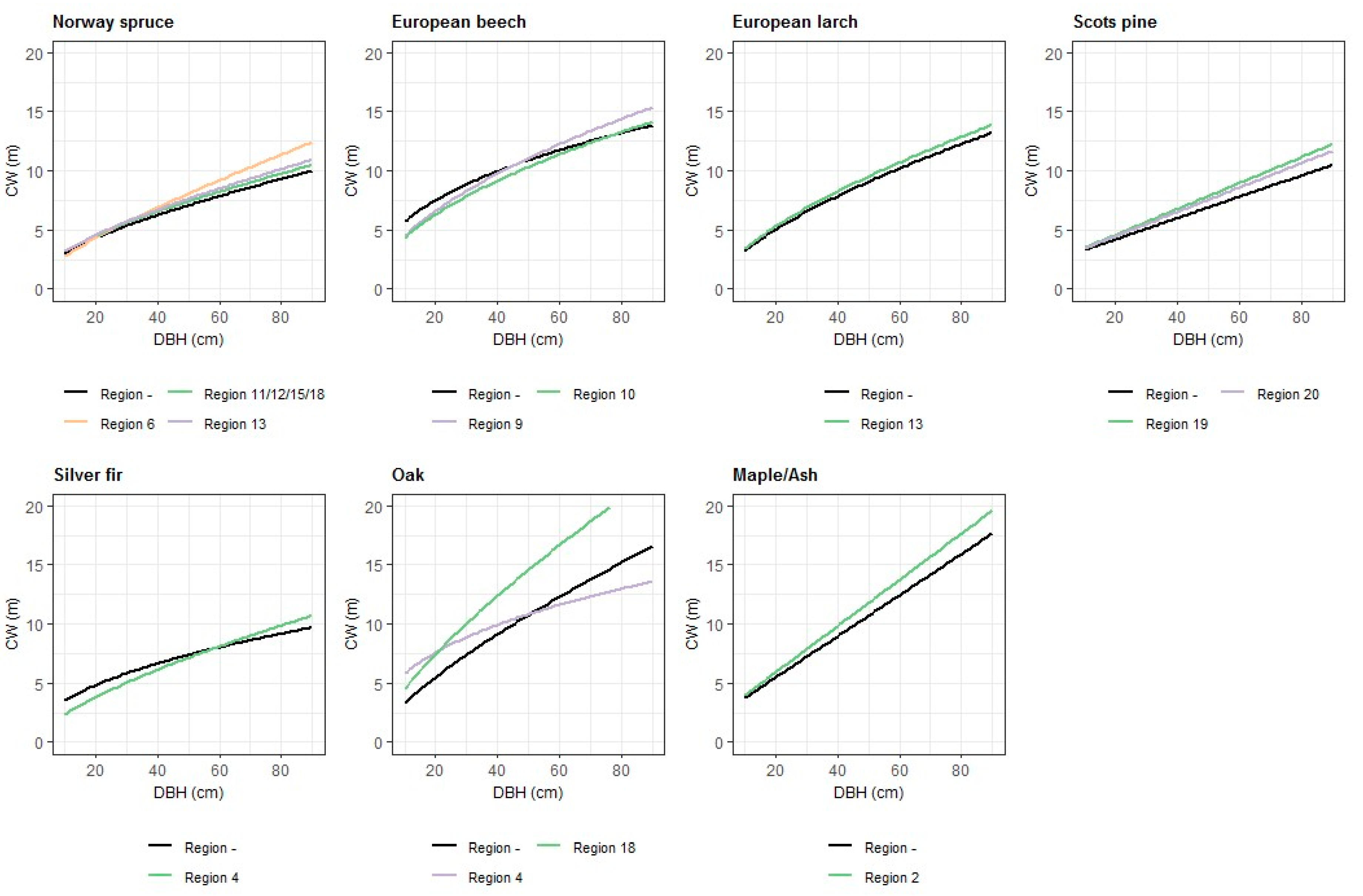
Site characteristics like ELEV, SL, and EXP had significant effects on the CW of a tree. The sea level of the site was incorporated through a linear and a quadratic term of ELEV, which were both significant. Data exploration using dot plots indicated that trees with a larger DBH reacted stronger to a change in ELEV than trees with a small DBH. This was supported by significant interaction terms between ELEV, ELEV² and DBH. In pure spruce stands, the optimum was about 700 m. The significant interaction between the cosine of EXP and SL indicated that spruce trees growing on a site, which is exposed to south–east, had larger CWs than trees growing on sites exposed to north–west. The sine term of the slope-aspect transformation was not significant, but was added in the model to achieve a proper continuous behavior of the circular function [37]. Differences between growth regions (Figure 1) were considered by including dummy variables, which were affecting the intercept, for Region_6 (eastern edge of the Alps with subillyric climate) and Region_11/12/15/18 (northern central Alps, western part of the northern central Alps, southern central Alps and southeastern edge of the Austrian Alps) and dummy variables, which were affecting the logarithmic term of DBH, for Region_6 and Region_13 (central Alps).

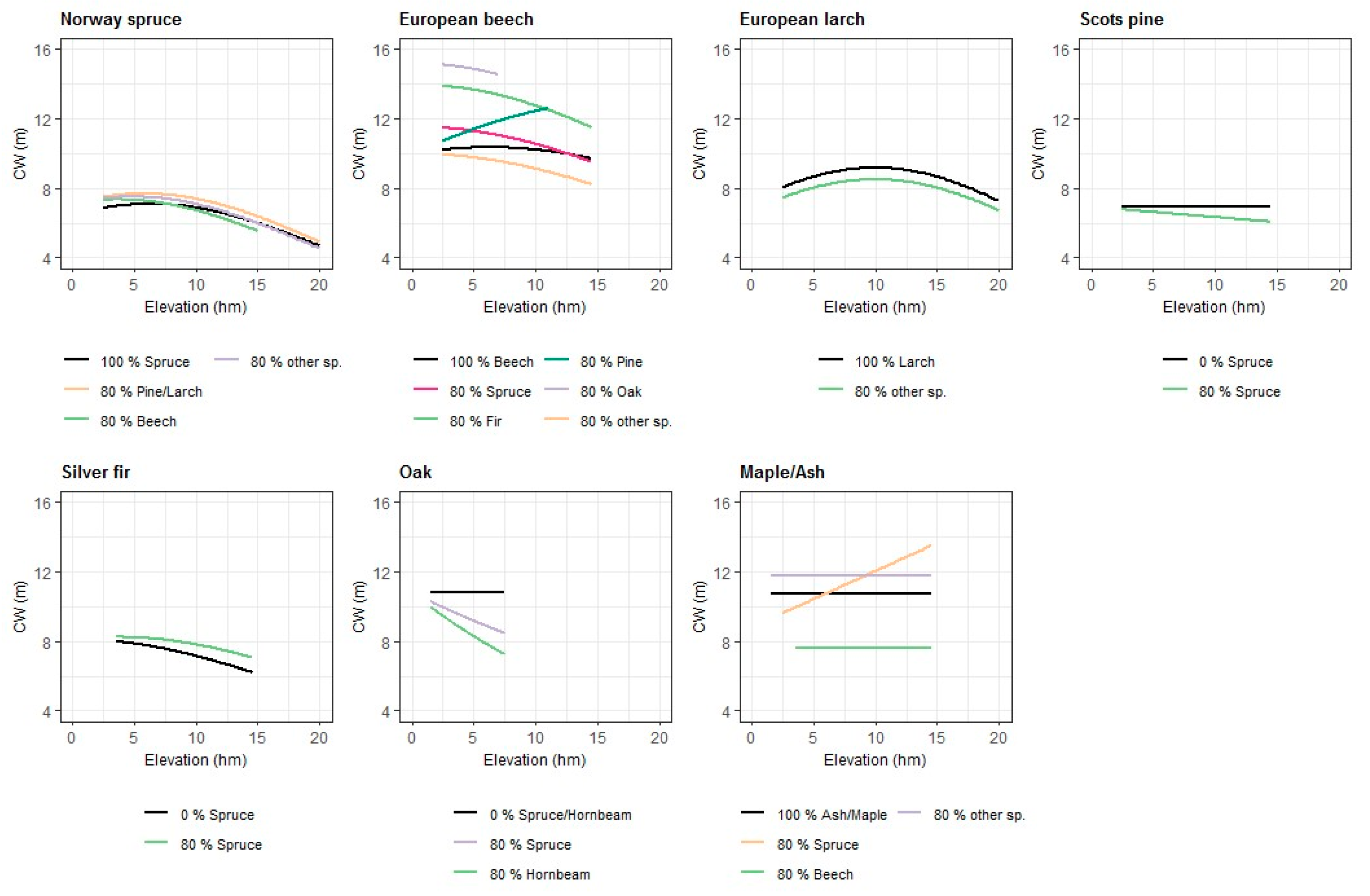
The effect of the species composition (Figure 2) of the stand on CW was described by the Norway spruce’s own proportion of the basal area (PS_1), the interaction between ELEV and PS_1, the summed proportion of Scots pine and European larch (PS_3/4), and the proportion of European beech (PS_10). In the model for Norway spruce, a square root transformation of all the species’ proportion parameters produced the best fit statistics. The own proportion of Norway spruce affected the CW of a tree in a negative way on sites below 1400 m a.s.l. (above sea level). The higher the proportion of Norway spruce in a stand, the lower was the CW. This effect was declining with increasing ELEV of the site. The effect of the proportion of Scots pine and European larch (PS_3/4) with its interaction with ELEV was significantly positive. With an increasing proportion of European larch and Scots pine, the CW was increasing. This effect was slightly decreasing with increasing elevation. The proportion of European beech (PS_10) had a positive effect on CW on lower sites below 800 m a.s.l, and a negative effect on higher sites.

The best performance of the CW model for silver fir was achieved through a logarithmic transformation of both the dependent variable and the independent variables DBH and H/D, respectively. The parameter estimates for the different transformations of CR were not significant.

EXP and SL had no significant effects on CW. The significant and negative parameter estimate of ELEV squared showed that in higher altitudes the CWs of silver fir trees were smaller than for trees on lower sites. The development of CW depending on DBH was different for trees in growth region 4 (western part of the hills and plain between the Alps and the Danube), observed by significant parameter estimates for the dummy variables affecting the intercept and the DBH variable. The significantly positive interaction between the relative proportion of Norway spruce (PS_1) and ELEV indicated that CW was increasing with a rising share of Norway spruce in the stand. This effect was stronger in high altitudes than in low altitudes.

The CW model with a logarithmic transformation of the dependent variable CW and independent variable DBH was also the best variant for European larch. H/D was incorporated as a quadratic term and CR by a logarithmic transformation. All of these variables were significant. Trees in Region_13 had a slightly wider CW than trees in the remaining growth regions which were taken into account by dummy variables affecting the intercept of the model.

ELEV was integrated into the model via a linear and a quadratic term and had a significant effect on CW. Up to the elevation of 1000 m a.s.l., CW was increasing; above this maximum CW was declining. The aspect and slope of the site had no significant effects on the CW of European larch. The significantly negative parameter estimate of PS_3 squared (larch’s own proportion of basal area) indicated that single European larch trees had a smaller CW in pure stands or in stands with a high proportion of European larch than trees growing in a stand with a low share of European larch.

For Scots pine, a transformation of CW and DBH was not necessary and the linear variant explained best the CW-DBH relationship. The square root-transformed H/D and CR had significant effects on CW, whereby increasing H/D and decreasing CR caused a decline in CW. It was not possible to prove that site characteristics, like ELEV, EXP, and SL, had an effect on the CW of single Scots pine trees. For trees in growth region 19 (granite hills on the eastern edge of the Alps) and 20 (south-eastern hills and terraces), the increase of CW with rising DBH was higher than for trees in the remaining growth regions, which was indicated by significant parameter estimates for the respective dummy variables.

The significantly negative interaction effect between the squared PSL_1 and ELEV showed that CW is declining with increasing share of Norway spruce in the stand and increasing elevation of the site. For the calculation of the relative tree species’ proportions, only those trees were taken into account, which reached the subject tree’s crown layer. The use of PSL_x brought an improvement in the model performance.

The common CW (Figure 3) model for the remaining coniferous species was kept simple and the species composition of the stand was not considered. Possible differences between species were tested by dummy variables affecting the intercept and the DBH for the different species. However, they were not significant. Higher ELEV had a significantly negative effect, and also EXP and SL had a significant influence on the tree’s CW. The maximum CW was reached, if the site was exposed to east and the minimum, if the site was exposed to the west. The sine term of the slope-aspect transformation was significant in contrast to the cosine term. However, the cosine term was also kept in the model.

3.2. Crown Width Models for Broadleaf Species

The development of complex models for the tree’s crown width was possible for European beech (Fagus sylvatica) and for oak species (Quercus sp.). Because of too few observations for maple, one common model for ash (Fraxinus excelsior) and maple species (Acer sp.) was parameterized. Non-significant dummy variables for maple species, which were affecting the intercept and DBH, supported the assumption that these species have a similar relationship between DBH and CW. For the remaining broadleaf species, a generic and simpler model without considering species composition of the stand was parameterized. Parameter estimates can be found in

Table 5. Parameter estimates of the mixed-effects CW models for broadleaf species. The dependent variable CW and DBH of the CW model for Maple and Ash species and for the remaining broadleaf species were not transformed. All shown estimates were significant (p-value < 0.05), except values printed in italics.

Tree Species	Fagus sylvatica	Quercus sp.	Acer/Fraxinus sp.	Other sp.
Depend Variable	ln(CW)	ln(CW)	CW	CW
Intercept	1.0910323	−1.0471094	1.1865967	0.4423783
Region_4	-	1.3611911	-	-
Region_6	-	-	-	−1.3161855
Region_9	−0.5924605	-	-	-
Region_10	−0.5657388	-	-	-
Region_21	-	-	-	−0.9284775
Region_18	-	0.304054	-	-
SP_12	-	-	-	2.1919433
SP_15/16	-	-	-	3.7354244
SP_18/23/27	-	-	-	1.3092625
DBH	-	-	0.1735585	0.1683018
Region_2 *DBH	-	-	0.021643	-
Region_8 * DBH	-	-	-	0.0722409
SP_15/16 * DBH	-	-	-	−0.1101649
SP_26 * DBH	-	-	-	−0.0224963
ln(DBH)	0.4036294	0.7315097	-	-
Region_4 * ln(DBH)	-	-0.3467259	-	-
Region_9 * ln(DBH)	0.1551168	-	-	-
Region_10 * ln(DBH)	0.1305651	-	-	-
H/D	−0.0029587	-	-	-
CR	-	-	3.3979624	2.3711534
ln (CR)	0.1684201	-	-	-
sqrt (CR)	-	0.7273862	-	-
ELEV²	−0.000946	-	-	−0.0059434
cos (EXP) * SL	0.00073	-	-	−0.0026763
sin (EXP) * SL	0.0005842	-	-	0.0166171
PSL_1	0.1809567	-	-	-
PSL_1²	-	-	−4.662721	-
PSL_2²	0.5235613	-	-	-
PSL_11²	0.6546167	-	-	-
PSL_13/14²	-	-	−1.1155706	-
sqrt (PSL_10)	-	-	2.4700418	-
PS_1 * ELEV	-	−0.0405627	-	-
PS_12 * ELEV	-	−0.0660866	-	-
PSL_1² * ELEV	-	-	0.5035608	-
PSL_4² * ELEV	0.0485298	-	-	-
PSL_10² * ELEV	0.0118516	-	-	-
sqrt (PSL_10) * DBH	-	-	−0.1433859	-

.

For European beech, the best model performance was reached through a transformation of the dependent variable CW and the independent variables DBH and CR with the natural logarithms. H/D was incorporated as a linear predictor and was significantly negative. The site characteristics ELEV, EXP and SL had a significant effect on the tree’s CW. The altitude of the site had a weak effect on CW in pure beech stands, but with a rising share of other species, the effect of ELEV was getting more noticeable (Figure 2). The parameter estimate of the sine term of the slope-aspect transformation was significant and indicating that beech trees on a site exposed to north–east have wider CWs as trees on sites exposed to south–west. Differences between growth regions were taken into account by the use of dummy variables for Region_9 (eastern part of the northern calcareous Alps) and Region_10 (western part of the northern calcareous Alps), which were significant. In Figure 1 can be seen that thin trees have smaller CWs in growth region 9 and 10, but the slope of DBH is higher resulting in wider CWs for thicker trees in comparison to the remaining regions. The species composition of the stand was incorporated by using PSL variables for the proportions of the different tree species and interaction variables with ELEV. The admixture of spruce resulted in higher CWs on sites at low altitudes. This effect was getting weaker with increasing ELEV. Higher proportions of oak species and silver fir result in wider CWs. The positive effect of Scots pine admixture is intensifying with increasing ELEV.

During the model building process for oak species, the logarithmic transformation of CW and DBH revealed to be the variant with the best model performance. Despite testing different transformations of H/D, this variable was not significant when CR was also included in the model. The use of the root-transformed CR was the best option with a significantly positive parameter estimate.

EXP and SL of the site had no significant effect on the tree’s CW. The site’s elevation (ELEV) didn’t have a significant and direct effect on CW, but via it’s interaction with the species proportion of Norway spruce (PS_1) and hornbeam (PS_12). The admixture of spruce and hornbeam had a negative effect on CW, which was intensified through increasing elevation. It could also be observed that the CW of oak trees in growth regions 4 and 18 reacts in a different way to increasing DBH in comparison to the remaining growth regions. The CW-DBH curve for region 4 is clearly flatter and the curve is steeper for region 18 (Figure 1).

For the common CW model for maple and ash species, a transformation of the dependent variable CW and the independent variables DBH, H/D and CR brought no improvement. CR had a significantly positive effect on CW and the parameter estimate for H/D was not significant when CW was also included in the model. EXP and SL of the site had no significant effect on CW. The altitude of the site had no direct effect, but influenced CW through its interaction with PSL_1. For growth region 2 (eastern pannonic semiarid region), the dummy variable affecting the DBH variable was significantly positive resulting in a steeper linear CW-DBH relationship. The incorporation of species proportion variables (PSL) revealed that the admixture of European beech (PSL_10) had a strongly negative effect on the CW of ash and maple trees, especially for trees with a higher DBH. On sites higher than 600 m a.s.l, CW is increasing with the rising proportion of Norway spruce. In lower altitudes, higher proportions of spruce had a negative impact on the tree’s CW. If only the own proportion of maple and ash species was decreasing, it had a positive effect on CW.

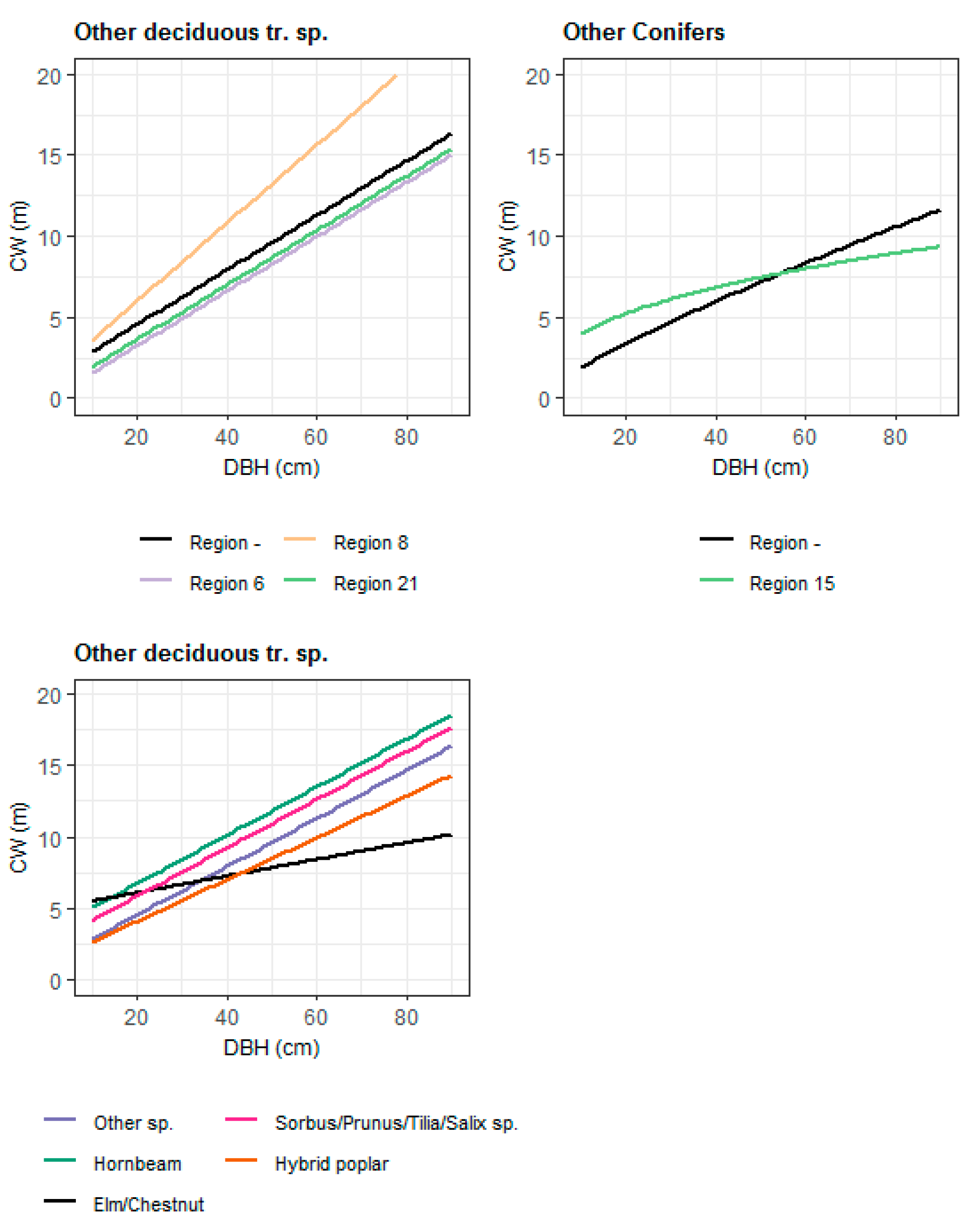
The common CW model for the remaining broadleaf species, which is not considering the species composition in the stand, was fitted with 452 observations. A transformation of the size variables and the dependent variable didn’t improve the model. To take differences between tree species into account, dummy variables for the various species, which were affecting the intercept and the DBH variable, were tested and included in the model. These differences between species can be seen in Figure 3. Site characteristics (ELEV, EXP, and SL) had significant effects on CW. With an increase in ELEV, the width of the tree’s crown is decreasing. The parameter estimates of the slope-aspect transformation, in which the sine term was significant, indicated that exposure of the site to the east had a positive effect on CW and exposure to the west had a negative impact.

4. Discussion

The 8900 tree crown width measurements of the ANFI revealed to be an excellent data basis to examine the impact of species mixture on a tree’s crown. Within the development of the linear mixed-effects CW models for different tree species, it was observed, that not only size and competition variables affected the CW of a tree strongly. The effects of site characteristics, like ELEV, SL and EXP, and the species composition of the stand, especially for broadleaf species, were found to be important predictors in CW models for eight different tree species.

Various approaches were used for modeling crown dimensions of trees. Simple linear or non-linear functions fitted with ordinary least square techniques were often used to describe the interrelationship between CW and DBH [13,15,37,38]. With these model techniques, it is not possible to consider a possible hierarchical structure of the data. Crown dimensions were usually assessed from trees growing in different stands and on different sites or environments. Therefore, a mixed-effect modeling approach is the preferred method for developing CW models, which also is recommended by Fu et al. [7,17] and was used in several other studies [16,19]. More complex modeling techniques, which can also be applied for modeling crown width, are nonlinear seemingly unrelated regression (NSUR) and nonlinear simultaneous equations (NSE). These techniques were used and evaluated by Fu et al. [39] and Lei et al. [40], who underline the advantage to consider the additivity properties of crown components (along the main compass directions measured crown radii) in their studies. However, these techniques were not reasonable to use in our study, because the measurement directions of crown radii were oriented on the exposure of the site and not on the compass directions.

CW and DBH are strongly correlated and DBH can be used as a single predictor variable in CW models [16,37,41]. The data set used in this study covers a huge variety of forest stands, including dense and sparse stands. Due to this large variation in data, additional variables were needed. In our model CR and H/D were incorporated because they clearly reflect a tree’s competitive situation in the past. Simpler models, which have only DBH as predictor variables, often overestimate CW for dense stand and underestimate for sparse stands [24]. In several other studies [16,24,42], distance-dependent competition indices, for example, Hegyi’s index [43], were used to take the competition between the observed tree and the neighboring trees into account. However, the inclusion of a distance-dependent competition measure was no option because (i) the ANFI data were collected via angle count sampling and do not provide information about the real spatial relationships of the neighboring trees, and (ii) the developed CW models will be incorporated in the forest growth simulator CALDIS VB V0.1 [26], which is a distance-independent individual-tree growth simulator. Stand density measures such as SDI [44] can easily be calculated from NFI data, but we decided not to include such measures in our models for the following reason: Competition (density) measures, independent whether they are stand based or individual-tree based, distance-dependent or distance-independent, quantify the current competition load of the trees while crown parameters (CR) and tree size (DBH, H) characterize the competition that a tree had experienced in the past. For modeling dynamic processes like growth or mortality, competition (density) measures need to be included in the models since they characterize the current competition load of a tree. However, in our case, the dependent variable to be modeled was CW, which is also a static variable like the other tree size variables DBH, H and CR. All these variables are the result of a tree’s competitive situation in the past, and their incorporation seems to be more important than including measures of current competition (stand density). Moreover, by restricting to the quoted tree size variables, an over-parameterization of the CW models is avoided.

Possible differences between tree species in the two models for the remaining conifer and deciduous tree species were considered through the incorporation of dummy variables which are affecting the two most crucial variables, the intercept, and the DBH variable. In this way, it was possible to take major differences of the CW-DBH relationships between species into account, so that the resulting models are relatively representative for each species. Possible discrepancies might rather be caused by a low number of observations for the respective tree species and not because of an inappropriate method of model development.

A literature research revealed that there are only a few existing CW models [45], which consider elevation, aspect and slope of the site. In our study, these variables proved to be crucial for most of the modelled species, expect for Scots pine, Oak species and Ash/Maple species. Regional differences in the CWs of trees were also observed by Hasenauer [45], who investigated crown dimensions of open-grown trees of different species in Austria. In this study Hasenauer [45] also used elevation, slope and aspect as site descriptors. However, in contrast to our study Hasenauer [45] referred to the so-called growth districts according to Mayer [46] while we used the growth regions according to Jelem and Kilian [28]. In both studies, the regional effects on CW were included by dummy variables. Another way to consider site quality is to incorporate the dominant height or dominant DBH of the stand in combination with the stand age [19] or to include the site index [16,17]. However, this was not possible in our study, because stand or tree age was not assessed within the Austrian NFI. Instead, we referred to the site descriptors ELEV, SL, EXP and growth region as this has already been done for the development of the PROGNAUS [47] and CALDIS VB V0.1 [26] growth functions.

Many recent studies underline that crown structure and crown dimensions, like crown length or width, can vary among pure and mixed forest stands [20,21,22,23]. If crown models are used to estimate biomass or canopy cover in both pure and mixed stands, it is necessary that they are able to reproduce the effects of mixture. Only a few crown models consider the species composition of the stand or distinguishing between pure and mixed stands [21,24]. In our study, the shade-tolerant conifer species Norway spruce and silver fir mainly reacted with wider CWs to increasing basal area proportion of admixed tree species. For Norway spruce, the own proportion of spruce had a negative effect on the CW of the observed trees indicating that spruce experienced the largest competitive effects from intraspecific competition. Light demanding species, Scots pine and European larch, affected the CW of Norway spruce positively. For the silver fir CW model, only an admixture of spruce had a significant effect and affected the CW positively. These findings are in concordance with the observations of Thorpe et al. [24]. In their crown radius models for Abies alsiocarpa, Pinus contorta and Picea glaucy × engelmanii, they used species-specific competition coefficients and could observe that shade tolerant species like fir and spruce were more competitive than the light-demanding pine. The results of our CW models European larch and Scots pine indicated a contrary behavior of light-demanding conifer species. An admixture of other tree species decreased the CW of larch and trees in pure larch stands showed wider crowns. For the Scots pines CW model, only the variable for the interaction between the proportion of spruce in the stand and the altitude was significant and a higher share of spruce affected CW negatively. These findings also suggest that shade-tolerant species were more competitive and interspecific competition lead to a stronger decrease in CW of larch and pine trees than intraspecific competition. The results of the CW models for European beech and Oak species also indicated that the shade-tolerant beech reacted positively to an admixture of spruce, pine, fir and oak and that light-demanding oak species reacted negatively to increasing share of spruce and hornbeam. Yoshida and Kamitani [25] investigated the interspecific competition among Fagus crenata, Quercus crispula and Magnolia obovata in Japan and observed that shade-tolerant species had an advantage in interspecific competition in mixed-species stands. The shade-tolerant Fagus crenata was more competitive and had a deeper crown depth and a higher leaf area index than the intermediate shade-tolerant Quercus crispula. Species composition had an unclear effect in the CW model for maple and ash species in our study. A higher admixture of beech reduced CW strongly, but a higher share of spruce had a strongly positive effect on CW of maple and ash trees in high altitudes above 700 m a.s.l. The comparison of our CW models for broadleaf and coniferous tree species shows that broadleaf trees generally reacted stronger to a change in species composition. A possible reason is that broadleaf trees have more plastic crowns and can react with more asymmetric crown shapes to the neighboring trees [48].

Most of our CW models incorporate species composition of the stand as interaction effects between the proportion of basal area and elevation of the site. A disadvantage of this approach is that a change in the distribution of different tree species due to climate change [49,50] might lead to a distortion of the interaction between elevation and species composition. For example, the CW model for Scots pine is only able to describe the effect of the admixture of Norway spruce in the stand. In the future, it can be that a tree species other than Norway spruce occurs in combination with Scots pine and has an effect on the CW of Scots pine trees. Because the common appearance of these two species was not present in our data set, the developed CW model would not be able to predict this potential effect. This has to be considered when using our CW models in long term forest growth simulations using climate-sensitive simulators. Our models cannot reflect possible climate-related changes in the competitive relationship among tree species. In simulation scenarios in which tree species distribution and composition change over time, the developed CW models might extrapolate leading to an overestimation of the effect of species composition. A validation of the developed CW models was not possible so far, because independent data sets with crown measurements from trees growing in mixed forests were not available.

5. Conclusions

In this study, nine models were developed to describe the crown width of individual trees of different species growing in Austria. Due to the hierarchical structure of the data set, the models adopt a linear mixed effects approach with random intercepts and sample plot as random factor. The CW models for conifer species explained between 72 and 83% of the variance (conditional R²) and the CW models for broadleaf species between 76 and 86%. For Norway spruce, silver fir, Scots pine, European larch, European beech, oak species and ash/maple species it was possible to develop CW models that are able to reflect the effect of species composition of the stand. The respective relative tree species’ proportions of basal area together with the interaction effects with the altitude of the sites revealed to be suitable variables to describe the effect of species composition. CWs of shade tolerant species showed a mainly positive reaction to admixture and light demanding species reacted with decreasing CWs. Broadleaf trees were stronger affected by the species composition than conifers.

References

- Reinhardt, E.; Crookston, N.L.; Beukema, S.J.; Kurz, W.A.; Greenough, J.A.; Robinson, D.C.E.; Lutes, D.C. Purpose and Applications. The Fire and Fuels Extension to the Forest Vegetation Simulator: Updated Model Documentation; Reinhardt, E., Crookston, N.L., Eds.; U.S. Department of Agriculture, Forest Service and Rocky Mountain Research Station: Fort Collings, CO, USA, 2010; pp. 1–8.
- Crookston, N.L.; Dixon, E.D. The forest vegetation simulator: A review of its structure, content, and applications. Comput. Electron. Agric. 2005, 49, 60–80. [Google Scholar] [CrossRef]
- Castaldi, C.; Vacchiano, G.; Marchi, M.; Corona, P. Projecting nonnative douglas fir plantations in Southern Europe with the forest vegetation simulator. For. Sci. 2017, 63, 101–110. [Google Scholar] [CrossRef] [Green Version]
- Crookston, N.L.; Rehfeldt, G.E.; Dixon, G.E.; Weiskittel, A.R. Addressing climate change in the forest vegetation simulator to assess impacts on landscape forest dynamics. For. Ecol. Manag. 2010, 260, 1198–1211. [Google Scholar] [CrossRef]
- Hasenauer, H.; Monserud, R.A. Biased predictions for tree height increment models developed from smoothed ‘data’. Ecol. Model. 1997, 98, 13–22. [Google Scholar] [CrossRef]
- Biging, G.S.; Dobbertin, M. Evaluation of competition indices in individual tree growth models. For. Sci. 1995, 41, 360–370. [Google Scholar]
- Fu, L.; Sharma, H.; Hao, K.; Tang, S. A generalized interregional nonlinear mixed-effects crown width model for Prince Rupprecht larch in northern China. For. Ecol. Manag. 2017, 389, 364–373. [Google Scholar] [CrossRef]
- Monserud, R.A.; Sterba, H. A basal area increment model for individual trees growning in even- and uneven-aged forest stands in Austria. For. Ecol. Manag. 1996, 80, 57–80. [Google Scholar] [CrossRef]
- Ledermann, T.; Neumann, M. Biomass equations from data of old long-term experimental plots. Austrian J. For. Sci. 2006, 1, 47–64. [Google Scholar]
- Carbalho, J.P.; Parresol, B.R. Additivity in tree biomass components of Pyrenean oak (Quercus pyrenaica Willd.). For. Ecol. Manag. 2003, 179, 269–276. [Google Scholar] [CrossRef]
- Krajicek, C.L.; Brinkman, K.A.; Gingrich, S.F. Crown competition—A measure of density. For. Sci. 1961, 7, 35–42. [Google Scholar]
- Paulo, J.A.; Faias, S.P.; Ventrua-Giroux, C.; Tome, M. Estimation of stand crown cover using a generalized crown diameter model: Application for the analysis of Portuguese cork oak stands stocking evolution. iForest 2015, 9, 437–444. [Google Scholar] [CrossRef] [Green Version]
- Shaw, J.D. Models for Estimation and Simulation of Crown and Canopy Cover. In Proceedings of the Fifth Annual Forest Inventory and Analysis Symposium, New Orleans, LA, USA, 18–20 November 2003; U.S. Department of Agriculture Forest Service: Washington, DC, USA; pp. 183–191. [Google Scholar]
- Pukkala, T.; Becker, P.; Kuuluvainen, T.; Oker-Blom, P. Predicting spatial distribution of direct radiation below forest canopies. Agric. For. Meteorol. 1991, 55, 295–307. [Google Scholar] [CrossRef]
- Elmungheira, M.I.; Elmamoun, H.O. Diameter at Breast Height—Crown Width Prediction Models for Anogeissus Leiocarpus (DC.) Guill & Perr and Combretum Hartmannianum Schweinf. J. For. Prod. Ind. 2014, 3, 191–197. [Google Scholar]
- Sharma, R.P.; Vacek, Z.; Vacek, S. Individual tree crown width models for Norway spruce and European beech in Czech Republic. For. Ecol. Manag. 2016, 366, 208–220. [Google Scholar] [CrossRef]
- Fu, L.; Sun, H.; Sharma, R.P.; Lei, Y.; Zhang, H.; Tang, S. Nonlinear mixed-effects crown width models for individual trees of Chines fir (Cunninghamia lanceolata) in south-central China. For. Ecol. Manag. 2013, 302, 210–220. [Google Scholar] [CrossRef]
- Davies, O.; Pommerening, A. The contribution of structural indices to the modelling of Sitka spruce (Picea stichensis) and birch (Betula spp.) crowns. For. Ecol. Manag. 2008, 256, 68–77. [Google Scholar] [CrossRef]
- Xu, H.; Sun, Y.; Wang, X.; Wang, J.; Fu, Y. Linear mixed-effects models to describe individual tree crown width for China-fir in Fujian Province, Southeast China. PLoS ONE 2015, 10, e0122257. [Google Scholar]
- Jucker, T.; Bourlaud, C.; Coomes, D.A. Crown plasticity enables trees to optimize canopy packing in mixed species forests. Funct. Ecol. 2015, 29, 1078–1086. [Google Scholar] [CrossRef] [Green Version]
- Pretzsch, H. The effect of tree crown allometry on community dynamics in mixed-species stands versus monocultures. A review and perspectives for modeling and silvicultural regulation. Forests 2019, 10, 810. [Google Scholar] [CrossRef] [Green Version]
- Sterba, H.; Dirnberger, G.; Ritter, T. Vertical distribution of leaf area of European larch (Larix decidua Mill. And Norway Spruce (Picea abies (L.) Karst.) in pure and mixed stands. Forests 2019, 10, 570. [Google Scholar] [CrossRef] [Green Version]
- Barbeito, I.; Dassot, M.; Bayer, D.; Collet, C.; Drössler, L.; Löf, M.; Rio, M.; Ruiz-Peinado, R.; Forrester, D.I.; Bravo-Oviedo, A.; et al. Terrestrial laser scanning reveals differences in crown structure of Fagus sylvatica in mixed vs. pure European forests. For. Ecol. Manag. 2017, 405, 381–390. [Google Scholar] [CrossRef]
- Thorpe, H.C.; Astrup, A.; Trowbridge, A.; Coates, K.D. Competition and tree crowns: A neighbourhood analysis of three boreal tree species. For. Ecol. Manag. 2010, 259, 1586–1596. [Google Scholar] [CrossRef]
- Yoshida, T.; Kamitani, T. Interspecific competition among three canopy-tree species in a mixed-species even-aged forest of central Japan. For. Ecol. Manag. 2000, 137, 221–230. [Google Scholar] [CrossRef]
- Ledermann, T.; Kindermann, G.; Gschwantner, T. National woody biomass projection systems based on forest inventory in Austria. In Forest Inventory-Based Projection Systems for Wood and Biomass Availability; Barreiro, S., Schelhaas, M.J., McRoberts, R.E., Kändler, G., Eds.; Springer International Publishing: Cham, Switzerland, 2017; pp. 79–95. [Google Scholar]
- Braun, M.; Fritz, D.; Weiss, P.; Braschel, N.; Büchsenmeister, R.; Freudenschuß, A.; Gschwantner, T.; Jandl, R.; Ledermann, T.; Neumann, M.; et al. A holistic assessment of greenhouse gas dynamics from forests to the effects of wood products use in Austria. Carbon Manag. 2016, 7, 271–283. [Google Scholar] [CrossRef]
- Jelem, H.; Kilian, W. Standortsaufnahme im rahmen der österr. Forstinventur–eine forstpolitische entscheidungshilfe. Allg. Forstztg. 1972, 83, 295–297. [Google Scholar]
- Bitterlich, W. Die Winkelzählprobe. Allg. Forst-u. Holzwirtaschtsztg 1948, 59, 4–5. [Google Scholar] [CrossRef]
- Pretzsch, H. Zum einfluß des baumverteilungsmusters auf den bestandeszuwachs. Allg. Forst-u. J. Ztg. 1995, 166, 190–201. [Google Scholar]
- Pinheiro, J.C.; Bates, D.M. Mixed-Effects Models in S and S-PLUS; Spring: New York, NY, USA, 2000; pp. 3–56. [Google Scholar]
- Bates, D.; Mächler, M.; Bolker, B.M.; Walker, S.C. Fitting linear mixed-effects models using lme4. J. Stat. Softw. 2015, 67, 1–48. [Google Scholar] [CrossRef]
- Kunetsova, A.; Brockhoff, P.B.; Christensen, R.H.B. lmerTest Package: Tests in linear mixed effects models. J. Stat. Softw. 2017, 82, 1–26. [Google Scholar]
- Wonn, H.T.; O’Hara, K.L. Height: diameter ratios and stability relationships for four Northern Rocky Mountain tree species. West. J. Appl. For. 2001, 16, 87–94. [Google Scholar] [CrossRef] [Green Version]
- Ledermann, T. A non-linear model to predict crown recession of Norway spruce (Picea abies [L.] Karst.) in Austria. Eur. J. For. Res. 2011, 130, 521–531. [Google Scholar] [CrossRef]
- Stage, A.R. An expression for the effect of slope, aspect and habitat type on tree growth. For. Sci. 1976, 22, 457–460. [Google Scholar]
- Sönmez, T. Diameter at breast height-crown diameter prediction models for Picea orientalis. Afr. J. Agric. 2009, 4, 215–219. [Google Scholar]
- Bragg, D.C. A local basal area adjustment for crown width prediction. North. J. Appl. For. 2001, 18, 22–28. [Google Scholar] [CrossRef] [Green Version]
- Fu, L.; Sharma, R.P.; Wang, G.; Tang, S. Modelling a system of nonlinear additive crown width models applying seemingly unrelated regression for Prince Rupprecht larch in northern China. For. Ecol. Manag. 2017, 386, 71–80. [Google Scholar] [CrossRef]
- Lei, Y.; Fu, L.; Affleck, D.L.R.; Nelson, A.S.; Shen, C.; Wang, M.; Zheng, J.; Ye, Q.; Yang, G. Additivity of nonlinear tree crown width models: Aggregated and disaggregated model structures using nonlinear simultaneous equations. For. Ecol. Manag. 2018, 427, 372–382. [Google Scholar] [CrossRef]
- Foli, E.G.; Alder, D.; Miller, D.G.; Swaine, M.D. Modelling growing space requirements for some tropical tree species. For. Ecol. Manag. 2003, 173, 79–88. [Google Scholar] [CrossRef]
- Grote, R. Estimation of crown radii and crown projection area from stem size and tree position. Ann. For. Sci. 2003, 60, 393–402. [Google Scholar] [CrossRef] [Green Version]
- Hegyi, F. A simulation model for managing jack-pine stands. In Growth Models for Tree and Stand Simulation; Fries, J., Ed.; Royal College of Forestry: Stockholm, Sweden, 1974; pp. 74–90. [Google Scholar]
- Reineke, L.H. Perfecting a Stand density index for even-aged forests. J. Agric. Res. 1933, 46, 627–638. [Google Scholar]
- Hasenauer, H. Dimensional relationships of open-grown trees in Austria. For. Ecol. Manag. 1997, 96, 197–206. [Google Scholar] [CrossRef]
- Mayer, H.; Eckerhart, G.; Nather, G.; Rachoy, J.; Zuckrigl, K. Die Waldgebiete und Wuchsbezirke Österreichs. Cbl. f. d. ges. Forstw. 1971, 88, 129–164. [Google Scholar]
- Ledermann, T. Description of PrognAus for Windows 2.2. In Sustainable Forest Management—Growth Models for Europe; Hasenauer, H., Ed.; Springer: New York, NY, USA, 2006; pp. 71–78. [Google Scholar]
- Krucek, M.; Trochta, J.; Cibulka, M.; Kral, K. Beyond the cones: How crown shape plasticity alters aboveground competition for space and light—Evidence from terrestrial laser scanning. Agric. For. Meteorol. 2019, 264, 188–199. [Google Scholar] [CrossRef]
- Hanewinkel, M.; Cullmann, D.A.; Schelhaas, M.J.; Nabuurs, G.J.; Zimmermann, N.E. Climate change may cause severe loss in the economic value of European forest land. Nat. Clim. Chang. 2013, 3, 203–207. [Google Scholar] [CrossRef]
- Dyderski, M.K.; Paz, S.; Frelich, L.E.; Jagodzinski, A.M. How much does climate change threaten European forest tree species distributions? Glob. Chang. Biol. 2018, 24, 1150–1163. [Google Scholar] [CrossRef]
Figure 1.
Effects of DBH (cm) and growth region on the CW (m) for different tree species in pure stands. The figures were produced using the parameter estimates for the fixed effects in Table 3 and Table 4. For variables, which are not shown in this figure, the mean values of the observed data were used.
Figure 2.
Effects of elevation (hectometre) and species composition in the stand (described by PS_x or PSL_x) on the CW (m) for different tree species. The figures were produced using the parameter estimates for the fixed effects in Table 3 and Table 4. For the DBH, a value of 50 cm was assumed. For other variables, which are not shown in this figure, the mean values of the observed data were used.
Figure 3.
Effects of DBH (cm) on the CW (m) of the remaining broadleaf and coniferous species, for which the number of observations was too small to calibrate CW models for each species. The differences between tree species and growth regions were incorporated by dummy variables.