How Are Green Spaces Distributed among Different Social Groups in Urban China? A National Level Study


1
Graduate School of Design, Harvard University, Cambridge, MA 02138, USA
2
Faculty of Social Science, University of Hong Kong, Pok Fu Lam, Hong Kong, China
*
Author to whom correspondence should be addressed.
Forests 2020, 11(12), 1317; https://0-doi-org.brum.beds.ac.uk/10.3390/f11121317
Submission received: 17 November 2020
/
Revised: 5 December 2020
/
Accepted: 6 December 2020
/
Published: 10 December 2020
(This article belongs to the Section Forest Ecology and Management)
Abstract
:The study analyzes the distributional equity of urban green space (UGS) among different social groups across all urban areas in China. Urban green space is measured in two ways: Park area per capita and vegetation coverage ratio within 1.6 km and 3.2 km featuring different ecosystem services they provide. Multiple regression analyses are conducted to assess relationships between different groups (children, the elderly, and migrant populations) and distributed UGS. Largely consistent to other national level studies, the nationwide analytical results indicate emerging social inequality of UGS during the urbanization of China, with a few nuances. A bi-fold pattern is observed in our case: Whilst areas with higher portions of children and senior people have less parks and high vegetation coverage, a marginalized group—internal migrant people, have more parks and low vegetation coverage in their vicinities. The results of regression analyses in different regions further shed light on revealing disparities of UGS in areas with varying socioeconomic development levels, geographical features, and urbanization paces. The implication of the study informs the decision makers to incorporate spatial patterns of social groups into green space guidance and evaluation for the purpose of promoting more equal development of UGS.
1. Introduction
As more than half of the world’s population lives in urban areas [1], urban green space (UGS) is receiving increasing attention and has been widely implemented to reduce the negative impacts of urbanization [2,3,4]. UGS refers to vegetated open spaces including parks, forests, waterfronts, community gardens, and streets populated with trees that is useful for the ecosystem in multiple ways [5]. It is widely acknowledged that parks provide diverse outdoor recreational spaces that can promote visitors’ social interactions, physical wellness, and even mental wellness [2,6,7,8,9,10]. Forests, trees on streets, green roofs, and other forms of vegetation in UGS can improve environmental quality in different ways via air purification, runoff mitigation, water and soil conservation, heat-island effect reduction, and noise cancellation [11,12,13,14]. With such positive benefits, UGSs, particularly large iconic parks, are known to raise the value of neighboring land and housing prices [15,16,17]. Forming a natural element of the urban system, UGSs in the form of wetland and countryside forests also serve as key wildlife habitats and migration stepping-stones for conserving local and global biodiversity [18,19].
However, empirical evidence shows that UGSs are not evenly distributed among different socioeconomic and demographic subgroups defined by income level, age, education, racial and ethnic disparity, and even immigration status [4,20,21,22,23,24,25,26]. These disparities in UGS distribution are considered an environmental justice issue and cause many problems with respect to public health and gentrification [2,27]. Equal access to such spaces could promote residents’ wellbeing, which could particularly benefit lower-income, marginalized people [4,28]. Even though ideal equality might not be practical, localities with a higher proportion of marginal groups should have access to the same amount of UGS, no matter their socioeconomic and demographic attributes [4,29].
The social inequality characterizing green space distribution is a particularly urgent matter in China. The country now accommodates more than half its population in urban areas [30], and over the past two decades, many cities have strived to invest significantly in afforestation projects including building new parks, renaturing waterfronts and planting trees on streets [31]. Park area per capita has increased from 3.7 m2 in 2000 to 14.1 m2 in 2019, and green space per resident (including all types of vegetation) in urban areas has grown from 39.1 m2 in 2000 to 86.9 m2 in 2019 [32]. UGS in China is still underdeveloped compared to other countries: the U.S. reports an average parkland area of 214 m2 in its 100 largest cities in 2019 [33], and each urban dweller in Europe has, on average, 18 m2 of parkland [34]. Although the park area per capita in China (11 m2 in 2010) is similar to that in Japan (10 m2), the area itself is still considerably lesser in China considering Japan’s doubled population density [35]. Moreover, such non-spatially explicit indicators often adopted by official sectors for UGS evaluation cannot reflect the spatial patterns of green spaces [36]. Though the national standard for UGS evaluation utilizes the park buffer coverage ratio as an additional indicator for measuring spatial service capacity, this method cannot trace the spatial distribution of different social groups within a city [37].
In addition, rapid urbanization and the fast-evolving socioeconomic statuses that accompany it might further cause unequal UGS distributions among different social groups. Previously, following the legacy of socialist urban planning, UGS was emphasized as being evenly distributed among all city residents [38,39]. However, after establishing a freer land market economy in the 1990s, the mechanisms of UGS provisions have changed. As land leasing revenue is gradually becoming a major source of local governmental income, the planning of UGS is often geared toward generating more tangible profit [40]. To raise the land value and attract more real estate development, UGSs (particularly large parks) are encouraged to act as stimulators more than mere public amenities and components of the ecosystem. For example, the Beijing municipality built the largest forest park to host the 2008 Olympic Games and subsequently attracted numerous high-end real estate developments [17]. Some cities even adopted policies to relocate existing UGSs to further, less desirable areas so as to allocate more central urban spaces for profitable real estate development, such as Wuhan’s “occupation and compensation” policy [41]. As a result, the implementation of UGS is often spatially distorted within city boundaries and can lead to an uneven distribution among social groups signaling potential environmental injustice, while the total quantity of green space might meet the requirements of upper-level urban planning.
Indeed, the emerging empirical studies, though limited in number, have identified a disparity in UGS distributions in China informed by social inequality [38,39,42,43]. However, most of these studies focus on investigating individual cities. Additionally, due to the varying geographical, socioeconomic, and even historical contexts, as well as diverse research methods, scales, and definitions of UGSs, current studies conducted in Chinese cities often generate divergent conclusions. Some empirical evidence suggests that vulnerable people can access more UGS. For example, research in Shanghai found that marginalized groups tend to access parks more frequently [39,44]. In Hangzhou, the local government’s investment in building parks tends not to discriminate between any social groups [38]. Another group of researchers returned opposing observations. An investigation in Beijing claimed that poor people living in lower-priced communities have fewer parks around [42]. A similar study in Shenzhen indicates that the number of parks is limited in socioeconomically disadvantaged districts, demonstrating the existence of park inequality [43].
These inconsistent results pose a challenge for decision making, planning, and the management of UGS at both local and national levels. The guidelines, regulations, and standards of cities’ UGS planning are decided by national departments, and local governments are responsible for making and implementing these plans. Quantity based indicators such as green space coverage, park area per capita, the coverage ratio of park buffers, etc. within urban boundaries are emphasized in national regulations and standards to guide and evaluate local urban greening implementations [37,45]. However, these indicators are insufficient for promoting an equal intra-urban distribution of green space among different subgroups leading to the abovementioned undesirable outcomes; more parks or green spaces might be provided to certain people within a city. Without any proper understanding of UGS distribution among subgroups across the nation, China’s decision-makers might encounter difficulty in promoting location-sensitive policies and evaluation standards effective for guiding equal green space plans and implementations. Such challenges warrant a national-level analysis utilizing comprehensive data and spatially explicit measuring approaches involving different subgroups.
Thus far, current national-level studies related to UGS in China focus on describing the spatial-temporal dynamics of the volume and patterns of UGS [46,47,48], exploring relationships between vegetation composition and varying ecosystem services [49,50], and unraveling the impacts of socioeconomic factors on UGS provisions and implementation [40,51,52,53], which do not involve assessing the disparity of how UGS are distributed among different social groups. Another strand of literature utilizes big data, capturing people’s actual locations—via social media geolocation check-in or cellphone location data—as an indicator of residents’ actual use of or exposure to UGS [54]. Though individual location data can reflect how people actually use UGS, these approaches are often criticized due to the biased selection of the sample: poor members of the population, children, and older generations might have little access to such digital equipment, thus such measures cannot fully take account of the comprehensive UGS distribution for the total urban population [55].
To mind the abovementioned gaps, this paper uses the township as a basic unit (smallest census unit available) in China to measure UGS inequality among different subgroups across the country. We adopted two indicators to measure the distribution of UGS among urban dwellers: park area per capita and vegetation coverage ratio within 1.6 km and 3.2 km from the township centroid. The regional disparities in the inequality of UGS distribution are compared across varying levels of economic development, urbanization paces, and geographical conditions of cities in different regions [52]. The research paints a broad picture of the current distributional equity of UGS to inform the nation’s decision-makers in promoting location-specific and user-oriented evaluation and guiding standards in order to pursue equally distributed UGS in different subgroups and to mitigate environmental injustice at large.
2. Data and Methods
2.1. Data Collection and Handling
2.1.1. Study Area
The paper focuses on urban areas in China. Within an administrative border of a city, there are different types of subdistricts (townships) such as one or more central urban or town, populated urban-rural, rural, and nonresidential preserved subdistricts [56]. The township is the smallest census unit available with records of socioeconomic and demographic data. An area can be classified as urban based on the official urban-rural code, which is separately documented in the subunits of townships (but these subunits’ census records are not available). For example, a township is comprised of several smaller level communities (e.g. Juweihui in an urban area, Cunweihui in a rural area, etc. in Chinese), some of which are classified as urban and others rural. To filter urban areas, we include those township census units whose subunits are all coded as “urban core”, “town core”, “urban-rural fringe”, or “town-rural fringe” [57]. This approach includes fully developed central urban areas as well as the urban edges—the frontline of urban expansion. Considering the rapid urbanization of the past two decades, it is possible that the official codes might not fully capture the urbanized areas in China. To avoid this gap, we adopted two additional metrics to determine urban areas: one, according to a previous study [58], uses a population density of 1,000 people per km2 of township area, and the population density comes from a Landscan project [59]; the other selects the townships within urban land use borders based on satellite images [60]. Townships that met at least one of the three metrics and had at least one park within 1.6 km from their centroid point were included in the final sample. A total of 6,178 townships were considered to be urban areas out of a total of 43,576 census units, and the population involved was 396.2 million people, accounting for 28.5% of the total population of China in 2010 [61]. See Figure 1 for the distribution of the selected townships as urban areas.
2.1.2. Distribution of Urban Green Space
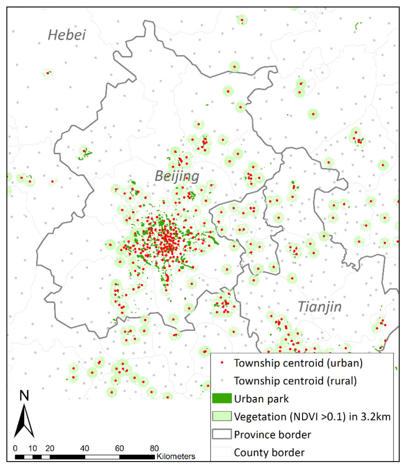
This study measures the distribution of UGS with two approaches: (1) the parks area per capita and (2) the coverage of all kinds of vegetation. The first indicator measures general recreational services of green space given that parks are the major accessible vegetated spaces for people’s outdoor activities in Chinese cities. The vegetation coverage evaluates coverall quantity of green space at township level. See Figure 2 for the layered park and total vegetation coverage distribution using townships in Beijing as an example.
Parks
The park data are extracted from two commercial map guide service companies—Gaode Map and Google Earth. First, the geo-locations of parks are extracted from Gaode Map, which only records the locations and entrances of parks, classifying any “park” as a Point of Interest (POI). One of the most appealing features of POI data is that it helps to identify the park locations which are accessible to the public while filtering out other types of green spaces that are used exclusively by certain groups. Many well-designed gardens exist in gated residential communities, fenced university campuses, or governmental compounds in Chinese cities, but they serve only the residents who have access. Plus, the POI is the only available data at the national scale which records the geolocations of parks. To ascertain the border of each park, the authors manually traced park patches based on high-resolution satellite historical images (mostly in the year 2010) using Google Earth. Where the images from 2010 were not available, the images from the most recent available year have been applied (within the range 2003–2014). The borders of the parks have been determined by the coverage of vegetation on designed pavements, roads, and recreational areas according to the official standard definition of urban parks [62]. In sum, 21,506 park patches were found in China. The total area was 240,891 hectares in the year 2010, which is similar to the official data, which noted 258,000 hectares in 2010 [63].
We adopted a simple and straightforward approach to measuring the distribution of parks. The total area of parks within 0.8 km, 1.6 km, and 3.2 km from the centroids of townships were calculated and divided by the township population. This approach is considered a cumulative opportunity metric, which assumes that more nearby parks offer more usable opportunities [64]. We used 800 m as a minimal search distance referring to a walking time of 10 mins, which is derived from a wider range of minimal distances used in other countries and China’s official sectors. A coverage distance of 500 m is the common indicator adopted by official sectors to measure the service capacity of park implementation [37]. Cities in European countries and the U.S. adopt distances ranging from 300 m to 1000 m as a standard distance to parks from households [3,4,20]. Researchers also include 1600 m, using a walking time of 20 mins as a reasonable journey duration for traveling to parks [22,39], which is particularly applicable in dense Chinese cities as people tend to tolerate and undergo longer journeys to parks [39]. Given the popularity of biking in Chinese cities, scholars also adopt 3.2 km as a threshold for those who bike to parks [39]. The selection of these three threshold distances allows us to compare our findings with similar studies focused on individual cities [4,22,38,39,42].
Vegetation Coverage
In addition to parks, this study also calculated all kinds of green space relying on satellite images. To compare all urban areas across China, this study utilized preprocessed 30 m resolution Lantsat 7 ETM + images, which was composited by median observation imageries from a set of quality-assessed growing season observations of four spectrum bands, specifically Landsat bands 3(RED), 4 (NIR), 5 (SWIR), and 7 (SWIR) [65]. A Normalized Difference of Vegetation Index (NDVI) value was utilized to identify all types of green spaces again within 0.8 km, 1.6 km, and 3.2 km buffers from township centroids. The pixels with NDVI values larger than 0.1 were counted as green spaces following a previous study using the same dataset [66], and the coverage ratio was then calculated for each buffer distance.
2.1.3. Socioeconomic and Demographic Variables
To discern how UGSs are distributed for different urban residents, socioeconomic and demographic data were collected for each township using official population census data in 2010 [61]. Due to the availability of data, we selected three indicators: percentage of the population aged lower than 14, percentage of the population aged higher than 65, and percentage of the population with a non-local Hu Kou (Chinese household registration) representing children, seniors, and internal migrant residents from other cities. The older generation and children travel to or use green spaces in different ways. For example, older people tend not to travel longer distances to parks in Shanghai [67], and most elderly people walk or cycle to parks within 10 mins from their homes in Hong Kong [68]. A study shows most children’s outdoor activities are in non-green urban environments, but they engage in more intense activities in outdoor green spaces [69]. Even though income level is the most direct indicator of socioeconomic status, such data is not open to the public at the township level. Instead, we use the Hu Kou status—Chinese household registration—as many scholars indicate that non-local Hu Kou populations are largely involved in unskilled, low-paid jobs and often suffer from discrimination in formal sector job markets and have limited access to many public welfare programs [70,71,72], thus rendering them a disadvantaged group in many studies [38,39,43].
County-level (the upper level of townships) socioeconomic indicators [73] are collected as controlled variables, given that different socioeconomic groups might prioritize other urban amenities over green spaces. For example, households with children might favor living in areas with more educational resources. Similarly, older urban residents tend to live close to healthcare amenities. Internal migrants usually aggregate in areas with more job opportunities [74,75]. Although data directly reflecting these amenities do not exist at the county level, we include, as substitutes, the percentage of employees in the healthcare industry, education industry, and tier 2 and tier 3 industries. The first two from that list can reflect county-level education and healthcare resources. Migrant workers usually seek jobs in tier 2 (e.g. construction, manufacturing) and 3 (e.g. retail, catering) industries [75]. The average housing area per capita was used as a proxy for the county’s income level [38]. Unemployment rate and population density were included for general socioeconomic development. In addition to the statistics shown in Table 1, we included provincial dummies as a control for the province-specific effects and major ecological-geographical zones across which the studied townships were located. Four ecological-geographical zones are demarcated in China: the East China Monsoon Region, the West China Arid Region, the Qinghai-Tibet Plateau, and the South China Tropical Island Region, according to temperature, precipitation, and topography [76].
2.2. Analytical Methods
2.2.1. The Spatial Disparity of UGS Distribution across China
Box plots were applied to present a broad picture of UGS distribution measured at the township level [77]. The spread of UGS distribution is useful for detecting inequality between different regions for further investigation regarding the attributable socioeconomic variables [4]. UGS distribution was mapped out at the provincial level. The box plots were drawn in Stata 15 and the maps produced in ArcGIS 10.8.1.
2.2.2. Multiple Regression Analyses
Multiple linear regressions were performed to understand the overall relationships between different social groups and the distribution of UGSs nationwide based on the following equation:
where represents the percentage of children, senior, or non-local internal migrants at township ; is the intercept; and are the area of park per capita and vegetation coverage; , , and are county-level socioeconomic factors, province and eco-geographical are dummies; and is error term; and is the number of township. Considering the influence of outliers, we excluded observations in the 1st and 99th percentiles of the variable accessible park areas from our sample in the final model. Sensitivity analyses were conducted using three different urban area definitions as mentioned in Section 2.1.1.
To detect any regional disparity in distribution of UGSs among different people, the regression analyses were separately conducted in four subregions. According to the national economic development plan, there are four regions: the east-coastal region, the central region, the western region, and the northeastern region in China, which reflect different paces of socioeconomic development [78]. The economic growth, the influx of internal migrants, urban area, and rate of urban expansion decrease from east-coastal and central cities to northwestern and western ones [40,74,79,80].
3. Results and Discussion
3.1. The Distribution of UGS across China
At the national level, the median amount of accessible park area per person was 3.1 m2 at the 1.6 km threshold and 12.2 m2 at the 3.2 km threshold. The maps in Figure 3a,c present a spatial distribution of the median amount of accessible park area across provinces. Both maps show that the northeastern and western provinces tend to have a higher area of parks near urban dwellers. The maps in Figure 4a,c show the median amount of vegetation coverage across provinces, in which the eastern-coastal provinces have more coverage than others. The results at the 0.8 km threshold level were excluded because most township units returned a zero value. This is due to the fact that the size of a township unit ranges widely, from about 2 km2 to 10 km2 in Beijing, for example [56]. Therefore, using the centroid of township unit measurement might not capture enough parks within an 800 m distance.
Box plots depicting parks are shown in Figure 3b,d. The widest spread of people’s access to parks was seen in Jilin Province at both measuring distances, while the narrowest was in Hainan Province at the 1.6 km threshold and Xizang (Tibet) at 3.2 km. In Figure 4, the box plots b and d reflect the median values and the spread of vegetation coverage in different provinces, both of which vary a lot across different provinces. The box plots identify the spatial patterns of UGS distribution for townships across different provinces.
The distribution of UGS is associated with an area’s degree of urbanization and economic development. The highest median values of park area aggregates were at the less-developed northeastern and western provinces, while the more developed eastern-coastal and central cities reported a lower median park area (a and c in Figure 3). This observation aligns with a previous study, which evidences the fact that economically advanced cities often have a negative impact on park development [40]. Unfortunately, those cities with a high median amount of park area also had a wider spread at the township level, suggesting that these provinces might bear a more unequal distribution of parks across their urban areas. The economically more developed and more urbanized eastern-coastal and central provinces had higher median values regarding their vegetation coverage ratios. This echoed previous research claiming that UGS is positively related to economic development [24,40,51,80]. The southern provinces had higher vegetation coverage than the northern and western areas due to the influence of bio-geographical conditions such as precipitation and sunlight radiation, etc. [51].
3.2. How UGSs Are Distributed among Different Social Groups
3.2.1. Nationwide Regression Analyses
The results of the regression analysis using all urban township units is presented in Table 2. The VIF (variance inflation factor) results confirm that there is no significant multicollinearity across all models (1.03 to 6.83). Sensitivity analyses involving different definitions of urban areas show consistent results (see Appendix A). The nationwide coefficients between different social groups and urban green space distributions are also presented in Figure 5. At both the 1.6 km and 3.2 km thresholds, the percentage of children is negatively associated with the number of accessible park areas, but a positive correlation is found for vegetation coverage (Model 1 & 2). A higher percentage of seniors in a population was aligned with a higher amount of both park area and vegetation coverage, but the effect was nonsignificant for parks (Model 3 & 4). On the contrary, at both the 1.6 km and 3.2 km radiuses, the percentage of non-local internal migrant residents was positively and significantly associated with the amount of accessible park area, whilst this relationship was significantly negative with regards to vegetation coverage (Model 5 & 6). In addition to the directions of correlation, the percentage of non-local residents had the highest correlations with a value of 0.063 for park area measured at the 1.6 km threshold. The county-level socioeconomic factors presented as expected. Townships with a higher proportion of kids tended to aggregate in counties with superior educational resources, though this effect is statistically insignificant. This might be attributable to the indicator we used to gauge educational resource integrated higher education, which was not desirable amenities for families with kids under age 14. Older people tended to live in the counties where there were more healthcare resources. Non-local internal migrants were attracted to counties with more job opportunities in the tier 2 and 3 industries, as migrants are more likely to be employed in industries related to construction, manufacture, and other low-skill service occupations [75].
The nation-wide regression analysis suggested the existence of social inequality in distributed park areas among different groups of the population in China. A bi-fold outcome was observed in our study across all urban areas of China. On one hand, children and senior populations had fewer parks and more vegetation coverage around their homes. A lower amount of accessible park area among younger populations has been detected in other individual cities such as Shanghai [39]. On the other hand, another group of disadvantaged people measured by local household registration status tended to have more parks, despite the low vegetation coverage in the vicinity of their residences. While contrasting the observations made in some European countries such as Germany [20], our results are consistent with national scale studies conducted in the U.S., which indicate that disadvantaged urban residents (measured according to income and education level) are likely to have more access to parks [4]. Our results also support the empirical evidence established on Shanghai, in which the marginalized, non-local population have more access to park areas [39].
The bi-fold pattern UGS distribution might have been the result of a mixed interaction among demographic distribution, urban sprawl, land use, and UGS provision mechanisms in Chinese cities. As cities expand their footprints, migrant residents from the rural hinterlands seek homes in peripheral urban areas due to the increased job opportunities in the peripheries and the unaffordable housing prices in the central areas [43]. Besides this, studies have identified a growing aggregation of senior members of the population in urban centers such as Beijing, Shanghai, Wuhan, and Guangzhou [81]. At the same time, city governments are installing large parks in the outskirts of cities where land prices are lower and empty land is more available. This is might be attributable to the land-based financing mechanisms for local government income revenue [40]. Especially after the land market’s opening to the private sector in the late 1990s, local governments’ incomes are largely derived from land lease revenues, and thus most municipalities tend to lease high-price inner-city land to private developers to gain more tangible profits by building housing or commercial estates instead of parks [40,74]. However, to meet the demand of the planned park volume, the government often reclaims areas on the outskirts of cities that costs less than renaturing dense city cores [38,41]. As a result, the peripheral non-local migrant workers—a disadvantaged group—have more parks in the vicinity of their homes, while older generations in the city core tend to lack parks, even though such an outcome is not intended.
Although the elderly and children have access to less park area, the community-attached gardens in the gated residential estates (reflected by vegetation coverage in our case) in China might provide alternative green spaces for their daily use. Gated communities have become a prevailing housing typology in urban areas since the late 1990s, and most of these were designed with usable areas of affiliated green space and vegetation-covered playgrounds exclusively for those who have access to or live in the community [82]. However, both the quality and size of the affiliated gardens vary according to housing prices as well as their locations within a city [17,39]. Old people or children living in high-end communities might have sizable private green spaces within their gated estates [39], whilst those living in dilapidated housing communities tend to have less usable inner green space. The migrant residents mostly living in city peripheries can find more large areas of parks around, even though the low-cost communities in which they live might lack sufficient private gardens (low vegetation coverage). Extreme cases can be found within affordable, “urban village” style housing enclaves built upon villages at the edge of cities during the period of rapid urban sprawl; these are commonly very dense and have only a few green spaces reserved for dwellers’ exclusive usage [72].
3.2.2. Regional Comparison
Regression analysis was conducted in each of the four regions and the results are shown in Table 3. The coefficients between different social groups and urban green space distributions are also plotted in Figure 6 by regions. All three demographic and socioeconomic indicators showed similar trends in the national-level analysis, but their strength and statistical significances varied widely. In all four regions, there was a negative relationship between the proportion of the younger population and the amount of accessible park area, among which the east-coastal region had the strongest correlation. This suggested there might be a nationwide inadequacy of park areas for children. Despite the fact that higher proportions of children were associated with more vegetation coverage in the east-coastal and central regions, these effects were marginal in the western and northeastern regions.
The percentage of senior members of the population was marginally correlated with park areas in all four regions, except the central region, which showed a positive and significant value at the 3.2 km threshold only. However, a more accessible park area at the 3.2 km threshold might be less useful for older generations, the majority of whom prefer to travel shorter distances to visit parks [44,67]. The vegetation coverage ratio at the 1.6 km and 3.2 km thresholds was significantly positively correlated with the proportion of older members of the population in all four regions. One possible explanation for this is the existence of well-greened urban centers. Cities with a longer history tend to have centers packed with historical green spaces [39], most of which are close to the homes of the elderly. The geographical pattern of cities—for example, a mountain in the middle of a city or a river passing through an urban center—might also contribute to more green spaces within the city center where more old people live, as these natural elements are often conserved as part of UGSs [81,83].
It is interesting to note that the proportion of non-local residents is significantly positively correlated with accessible park areas across the east-coastal and central regions. This further supports the trend of migrant workers clustering in suburban areas with more parks. The east-coastal and central cities have experienced the largest urban expansion in the past two decades, accumulating a large number of migrant workers from the western hinterland into the urban edge in the east-coastal and central cities [74,79]. In addition, urbanization has a longer history in these regions, which has left these already densified urban centers unable to accommodate both the influx of migrant populations and the installation of new parks. The pursuit of leasing expensive inner-city land to private sectors for profitable real estate development further drives local governments to install parks at the edge of the city, where the land is cheaper. However, vegetation coverage was negatively associated with the proportion of non-local migrant members of the population in all regions. This is likely because the disadvantaged migrant population, which is often comprised of low-income and less-skilled workers, might prioritize affordable housing and working opportunities over access to parks [71,75]. As a consequence, they tend to cluster in areas with less green space (captured as low vegetation coverage) in the dense affordable residential communities mentioned above.
3.3. Limitations and Areas for Future Research
The data used to calculate UGS distribution might serve as a potential limitation. The commercial map of POI data is unable to record pocket gardens and narrow linear waterfront and street-side public spaces, which provide residents with small but usable green spaces. To fill this gap, we calculated vegetation coverage using 30 m resolution satellite images. Still, using the NDVI to extract vegetation pixels could be subject to some inaccuracy. Even though the growing season Landsat imageries were selected, the 30 m resolution might overlook UGSs such as recently planted small street trees. However, we use the most comprehensive and consistent data to cover entire urban areas across the country. Given the census data availability, only three indicators were used to filter different social groups. The resolution of the socioeconomic dataset can hardly discern any finer grain (community or building level) socio-spatial disparity among urban populations. If it becomes available in the future, more systematic data in smaller census units with detailed socioeconomic information can be used to examine the (in)equality of UGS distribution in greater depth.
This study focuses on distributional equity of UGS in China. As many scholars argue, an equal spatial pattern does not constitute an equal process of UGS distribution [29,84]. Other factors such as the historical legacy of urban land use and planning, preexisting social segregation, and park funding mechanisms might all influence the UGS distributional patterns as urbanization continues [4,29,85,86]. This goes beyond the scope of our study but certainly highlights a new direction for future research, particularly in Chinese cities where the greening mechanisms and urbanization histories are vastly different from their Western counterparts. Lastly, we used a place-based indicator to measure park area and vegetation coverage. Yet, these metrics could not capture people’s perceptions toward UGSs nor their actual usage, as socioeconomic and psychological statuses might be influential in the process of analyzing actual usage [2,87]. A nation-wide survey or interviewing process might uncover such differences.
4. Conclusions
This study explores how UGS is distributed among different social groups at a relatively fine-grain township level across China. To the best of our knowledge, this is the first study to analyze all urban areas across the country, through which the emerging UGS inequality in Chinese cites is identified in terms of a few nuances examined in similar national studies worldwide. Our results indicate a bi-fold outcome of UGS distribution; the areas with higher portions of younger and senior populations tend to have fewer parks but more vegetation around their homes, while internal migrant residents—one vulnerable group—settle in areas with more park areas but with low nearby vegetation coverage. The regional comparison further highlights that a disparity of UGS distribution might reveal itself in areas with varying economic development and rates of urbanization. Such outcomes might result from interaction among different factors including land use, park funding mechanisms, green space planning, and regulations. At large, the regional comparison serves to expand our understanding of environmental justice issues with regards to UGS by drawing up a national-level study from a developing country that is concurrently experiencing rapid urban expansion and growing UGS investment.
These bi-fold results of diverging UGS distribution among different socioeconomic groups of people call for more location-oriented and user-specific afforestation guidance and evaluation standards. Instead of relying on traditional quantity-based indicators (such as green space per capita within city borders) to guide and assess UGS provision [37], integrating intra-urban spatial distributions of green space and the patterns of different residents into current planning regulations, guidelines, and evaluation processes could assist in reducing any potential (un)equal distribution of UGS, thus providing equal green space opportunities for urban dwellers. Additionally, decision-makers and planners should be alerted to the fact that afforestation processes that seek to mitigate inequality can generate undesirable outcomes such as gentrification, which hamper the positive effects of high park areas near marginal groups, particularly the non-local migrant people [2,17,88,89,90,91]. In order to avoid jeopardizing the equality of future UGS planning outcomes, potential factors causing inequality in UGS distribution—such as funding mechanisms, historical land use, and/or green space management—ought to be incorporated into the UGS distribution process; this will, however, require further nuanced studies on the detailed mechanisms driving UGS distribution outcomes.
Author Contributions
L.W. performed conceptualization, methodology, data collection, data analysis, validation, funding acquisition, and writing-original draft preparation. S.K.K. contributed to context framing, data collection, methodology, validation, and manuscript editing. All authors have read and agreed to the published version of the manuscript.
Funding
This research was funded by [China Scholarship Council] grant number [201608000011].
Conflicts of Interest
The authors declare no conflict of interest.
Appendix A

Table A1.
Sensitive analysis: regression for entire country using townships with population density larger than 1000 per km2.
Table A1.
Sensitive analysis: regression for entire country using townships with population density larger than 1000 per km2.
| VARIABLES | Model 1 Percentage of People under Age 14 | Model 2 Percentage of People under Age 14 | Model 3 Percentage of People above Age 65 | Model 4 Percentage of People above Age 65 | Model 5 Percentage of Internal Migrant Population | Model 6 Percentage of Internal Migrant Population |
|---|---|---|---|---|---|---|
| Park area accessible within 1.6 km | −0.019 *** | 0.001 | 0.064 *** | |||
| (0.002) | (0.002) | (0.009) | ||||
| Vegetation coverage rate within 1.6 km | 0.005 * | 0.025 *** | −0.201 *** | |||
| (0.003) | (0.003) | (0.015) | ||||
| Park area accessible within 3.2 km | −0.007 *** | 0.002 *** | 0.016 *** | |||
| (0.001) | (0.001) | (0.004) | ||||
| Vegetation coverage rate within 3.2 km | 0.012 *** | 0.018 *** | −0.199 *** | |||
| (0.003) | (0.003) | (0.015) | ||||
| Average housing area per capita | −0.010 | −0.008 | 0.023 *** | 0.019 ** | −0.072 * | −0.066 |
| (0.008) | (0.008) | (0.008) | (0.008) | (0.042) | (0.042) | |
| Unemployment rate | 0.041 *** | 0.038 *** | 0.132 *** | 0.135 *** | −0.690 *** | −0.700 *** |
| (0.008) | (0.008) | (0.008) | (0.008) | (0.042) | (0.042) | |
| Percentage of employed in education industry | −0.019 | −0.009 | −0.452 *** | −0.440 *** | 1.376 *** | 1.286 *** |
| (0.040) | (0.039) | (0.039) | (0.039) | (0.215) | (0.215) | |
| Percentage of employed in health industry | 0.151 * | 0.124 | 0.764 *** | 0.744 *** | −4.551 *** | −4.242 *** |
| (0.077) | (0.076) | (0.077) | (0.076) | (0.420) | (0.421) | |
| Percentage of employed in 2nd tier industry | −0.063 *** | −0.060 *** | −0.032 *** | −0.033 *** | 0.394 *** | 0.379 *** |
| (0.003) | (0.004) | (0.003) | (0.004) | (0.019) | (0.019) | |
| Percentage of employed in 3rd tier industry | −0.093 *** | −0.085 *** | −0.020 *** | −0.017 *** | 0.553 *** | 0.493 *** |
| (0.004) | (0.004) | (0.004) | (0.004) | (0.023) | (0.024) | |
| Log of Population density in 2010 | −0.403 *** | −0.316 *** | 0.730 *** | 0.632 *** | −2.159 *** | −1.942 *** |
| (0.056) | (0.054) | (0.055) | (0.054) | (0.304) | (0.298) | |
| Constant | 18.710 *** | 17.356 *** | −0.195 | 0.456 | 60.569 *** | 63.346 *** |
| (0.747) | (0.751) | (0.742) | (0.750) | (4.066) | (4.130) | |
| Observations | 4928 | 4910 | 4928 | 4910 | 4928 | 4910 |
| R-squared | 0.563 | 0.564 | 0.301 | 0.302 | 0.385 | 0.383 |
| Province Dummy | YES | YES | YES | YES | YES | YES |
| Ecozone Dummy | YES | YES | YES | YES | YES | YES |
Standard errors in parentheses. *** p < 0.01, ** p < 0.05, and * p < 0.1. Observations are excluded in the 1st and 99th percentiles of the variable accessible park areas in 1.6 km and 3.2 km.
Table A2.
Sensitive analysis: regression for entire country using townships within urban land use.
| VARIABLES | Model 1 Percentage of People under Age 14 | Model 2 Percentage of People under Age 14 | Model 3 Percentage of People above Age 65 | Model 4 Percentage of People above Age 65 | Model 5 Percentage of Internal Migrant Population | Model 6 Percentage of Internal Migrant Population |
|---|---|---|---|---|---|---|
| Park area accessible within 1.6 km | −0.019 *** | 0.002 | 0.061 *** | |||
| (0.002) | (0.002) | (0.010) | ||||
| Vegetation coverage rate within 1.6 km | 0.006 * | 0.019 *** | −0.186 *** | |||
| (0.003) | (0.003) | (0.016) | ||||
| Park area accessible within 3.2 km | −0.007 *** | 0.001 | 0.020 *** | |||
| (0.001) | (0.001) | (0.004) | ||||
| Vegetation coverage rate within 3.2 km | 0.013 *** | 0.013 *** | −0.177 *** | |||
| (0.003) | (0.003) | (0.016) | ||||
| Average housing area per capita | −0.017 ** | −0.018 ** | 0.020 ** | 0.016 ** | −0.038 | −0.025 |
| (0.008) | (0.008) | (0.008) | (0.008) | (0.044) | (0.044) | |
| Unemployment rate | 0.025 *** | 0.026 *** | 0.125 *** | 0.126 *** | −0.614 *** | −0.628 *** |
| (0.008) | (0.008) | (0.008) | (0.008) | (0.044) | (0.044) | |
| Percentage of employed in education industry | 0.014 | 0.017 | −0.468 *** | −0.457 *** | 1.214 *** | 1.134 *** |
| (0.041) | (0.041) | (0.041) | (0.041) | (0.224) | (0.224) | |
| Percentage of employed in health industry | 0.153 * | 0.121 | 0.852 *** | 0.842 *** | −4.902 *** | −4.622 *** |
| (0.080) | (0.080) | (0.079) | (0.079) | (0.435) | (0.435) | |
| Percentage of employed in 2nd tier industry | −0.065 *** | −0.061 *** | −0.032 *** | −0.033 *** | 0.412 *** | 0.397 *** |
| (0.004) | (0.004) | (0.004) | (0.004) | (0.020) | (0.020) | |
| Percentage of employed in 3rd tier industry | −0.091 *** | −0.083 *** | −0.020 *** | −0.018 *** | 0.563 *** | 0.510 *** |
| (0.004) | (0.005) | (0.004) | (0.004) | (0.024) | (0.025) | |
| Log of Population density in 2010 | −0.167 *** | −0.120 *** | 0.565 *** | 0.502 *** | −2.027 *** | −1.825 *** |
| (0.041) | (0.040) | (0.041) | (0.039) | (0.222) | (0.216) | |
| Constant | 17.224 *** | 16.226 *** | 0.907 | 1.447 ** | 59.055 *** | 61.129 *** |
| (0.696) | (0.703) | (0.690) | (0.694) | (3.781) | (3.831) | |
| Observations | 4613 | 4606 | 4613 | 4606 | 4613 | 4606 |
| R-squared | 0.564 | 0.564 | 0.310 | 0.312 | 0.383 | 0.382 |
| Province Dummy | YES | YES | YES | YES | YES | YES |
| Ecozone Dummy | YES | YES | YES | YES | YES | YES |
Standard errors in parentheses. *** p < 0.01, ** p < 0.05, and * p < 0.1. Observations are excluded in the 1st and 99th percentiles of the variable accessible park areas in 1.6 km and 3.2 km.
Table A3.
Sensitive analysis: regression for entire country using townships officially coded as urban.
Table A3.
Sensitive analysis: regression for entire country using townships officially coded as urban.
| VARIABLES | Model 1 Percentage of People under Age 14 | Model 2 Percentage of People under Age 14 | Model 3 Percentage of People above Age 65 | Model 4 Percentage of People above Age 65 | Model 5 Percentage of Internal Migrant Population | Model 6 Percentage of Internal Migrant Population |
|---|---|---|---|---|---|---|
| Park area accessible within 1.6 km | −0.020 *** | 0.007 *** | 0.039 *** | |||
| (0.002) | (0.002) | (0.012) | ||||
| Vegetation coverage rate within 1.6 km | 0.001 | 0.010 *** | −0.129 *** | |||
| (0.003) | (0.003) | (0.016) | ||||
| Park area accessible within 3.2 km | −0.009 *** | 0.003 *** | 0.015 *** | |||
| (0.001) | (0.001) | (0.005) | ||||
| Vegetation coverage rate within 3.2 km | 0.011 *** | 0.000 | −0.115 *** | |||
| (0.003) | (0.003) | (0.018) | ||||
| Average housing area per capita | 0.008 | 0.008 | −0.016 * | −0.019 * | 0.074 | 0.075 |
| (0.010) | (0.010) | (0.010) | (0.010) | (0.053) | (0.053) | |
| Unemployment rate | −0.011 | −0.009 | 0.170 *** | 0.170 *** | −0.805 *** | −0.820 *** |
| (0.009) | (0.009) | (0.009) | (0.009) | (0.047) | (0.047) | |
| Percentage of employed in education industry | −0.034 | −0.028 | −0.442 *** | −0.439 *** | 1.255 *** | 1.250 *** |
| (0.038) | (0.038) | (0.040) | (0.040) | (0.212) | (0.212) | |
| Percentage of employed in health industry | 0.217 *** | 0.189 ** | 0.727 *** | 0.740 *** | −4.365 *** | −4.243 *** |
| (0.075) | (0.075) | (0.079) | (0.079) | (0.417) | (0.419) | |
| Percentage of employed in 2nd tier industry | −0.048 *** | −0.045 *** | −0.034 *** | −0.036 *** | 0.336 *** | 0.330 *** |
| (0.004) | (0.004) | (0.004) | (0.004) | (0.023) | (0.023) | |
| Percentage of employed in 3rd tier industry | −0.073 *** | −0.067 *** | −0.024 *** | −0.026 *** | 0.508 *** | 0.476 *** |
| (0.004) | (0.005) | (0.005) | (0.005) | (0.024) | (0.025) | |
| Log of Population density in 2010 | −0.178 *** | −0.118 *** | 0.498 *** | 0.424 *** | −2.118 *** | −1.828 *** |
| (0.037) | (0.035) | (0.039) | (0.037) | (0.207) | (0.197) | |
| Constant | 17.045 *** | 16.057 *** | 1.946 ** | 2.857 *** | 64.714 *** | 64.186 *** |
| (0.732) | (0.740) | (0.769) | (0.773) | (4.055) | (4.116) | |
| Observations | 3905 | 3924 | 3905 | 3924 | 3905 | 3924 |
| R-squared | 0.531 | 0.533 | 0.344 | 0.348 | 0.345 | 0.341 |
| Province Dummy | YES | YES | YES | YES | YES | YES |
| Ecozone Dummy | YES | YES | YES | YES | YES | YES |
Standard errors in parentheses. *** p < 0.01, ** p < 0.05, and * p < 0.1. Observations are excluded in the 1st and 99th percentiles of the variable accessible park areas in 1.6 km and 3.2 km.
References
- United Nations. World Urbanization Prospects: The 2018 Revision; 2018; p. 30. Available online: https://www.un.org/en/events/citiesday/assets/pdf/the_worlds_cities_in_2018_data_booklet.pdf (accessed on 7 December 2020).
- Wolch, J.R.; Byrne, J.; Newell, J.P. Urban green space, public health, and environmental justice: The challenge of making cities ‘just green enough’. Landsc. Urban Plan. 2014, 125, 234–244. [Google Scholar] [CrossRef] [Green Version]
- Kabisch, N.; Strohbach, M.; Haase, D.; Kronenberg, J. Urban green space availability in European cities. Ecol. Indic. 2016, 70, 586–596. [Google Scholar] [CrossRef]
- Nesbitt, L.; Meitner, M.J.; Girling, C.; Sheppard, S.R.J.; Lu, Y. Who has access to urban vegetation? A spatial analysis of distributional green equity in 10 US cities. Landsc. Urban Plan. 2019, 181, 51–79. [Google Scholar] [CrossRef]
- Taylor, L.; Hochuli, D.F. Defining greenspace: Multiple uses across multiple disciplines. Landsc. Urban Plan. 2017, 158, 25–38. [Google Scholar] [CrossRef] [Green Version]
- Bertram, C.; Rehdanz, K. The role of urban green space for human well-being. Ecol. Econ. 2015, 120, 139–152. [Google Scholar] [CrossRef] [Green Version]
- Hong, W.; Guo, R. Indicators for quantitative evaluation of the social services function of urban greenbelt systems: A case study of shenzhen, China. Ecol. Indic. 2017, 75, 259–267. [Google Scholar] [CrossRef]
- Van den Berg, M.; van Poppel, M.; van Kamp, I.; Andrusaityte, S.; Balseviciene, B.; Cirach, M.; Danileviciute, A.; Ellis, N.; Hurst, G.; Masterson, D.; et al. Visiting green space is associated with mental health and vitality: A cross-sectional study in four european cities. Health Place 2016, 38, 8–15. [Google Scholar] [CrossRef]
- Picavet, H.S.J.; Milder, I.; Kruize, H.; de Vries, S.; Hermans, T.; Wendel-Vos, W. Greener living environment healthier people? Exploring green space, physical activity and health in the Doetinchem Cohort Study. Prev. Med. 2016, 89, 7–14. [Google Scholar] [CrossRef]
- Nutsford, D.; Pearson, A.L.; Kingham, S. An ecological study investigating the association between access to urban green space and mental health. Public Health 2013, 127, 1005–1011. [Google Scholar] [CrossRef]
- Zhang, B.; Xie, G.-d.; Li, N.; Wang, S. Effect of urban green space changes on the role of rainwater runoff reduction in Beijing, China. Landsc. Urban Plan. 2015, 140, 8–16. [Google Scholar] [CrossRef]
- Wu, J.; Xie, W.; Li, W.; Li, J. Effects of Urban Landscape Pattern on PM2.5 Pollution—A Beijing Case Study. PLoS ONE 2015, 10, e0142449. [Google Scholar] [CrossRef] [PubMed] [Green Version]
- Kremer, P.; Hamstead, Z.A.; McPhearson, T. The value of urban ecosystem services in New York City: A spatially explicit multicriteria analysis of landscape scale valuation scenarios. Environ. Sci. Policy 2016, 62, 57–68. [Google Scholar] [CrossRef]
- Fan, P.; Xu, L.; Yue, W.; Chen, J. Accessibility of public urban green space in an urban periphery: The case of Shanghai. Landsc. Urban Plan. 2017, 165, 177–192. [Google Scholar] [CrossRef]
- Crompton, J.L. The impact of parks on property values: Empirical evidence from the past two decades in the United States. Manag. Leis. 2005, 10, 203–218. [Google Scholar] [CrossRef]
- Czembrowski, P.; Kronenberg, J. Hedonic pricing and different urban green space types and sizes: Insights into the discussion on valuing ecosystem services. Landsc. Urban Plan. 2016, 146, 11–19. [Google Scholar] [CrossRef]
- Zheng, S.; Kahn, M.E. Does Government Investment in Local Public Goods Spur Gentrification? Evidence from Beijing. Real Estate Econ. 2013, 41, 1–28. [Google Scholar] [CrossRef]
- Forman, R.T.T. Urban Ecology: Science of Cities; Cambridge University Press: New York, NY, USA, 2014. [Google Scholar]
- Goddard, M.A.; Dougill, A.J.; Benton, T.G. Scaling up from gardens: Biodiversity conservation in urban environments. Trends Ecol. Evol. 2010, 25, 90–98. [Google Scholar] [CrossRef]
- Wüstemann, H.; Kalisch, D.; Kolbe, J. Access to urban green space and environmental inequalities in Germany. Landsc. Urban Plan. 2017, 164, 124–131. [Google Scholar] [CrossRef]
- Nesbitt, L.; Meitner, M. Exploring Relationships between Socioeconomic Background and Urban Greenery in Portland, OR. Forests 2016, 7, 162. [Google Scholar] [CrossRef]
- Talen, E. The Social Equity of Urban Service Distribution: An Exploration of Park Access in Pueblo, Colorado, and Macon, Georgia. Urban Geogr. 2013, 18, 521–541. [Google Scholar] [CrossRef]
- Rigolon, A.; Browning, M.; Lee, K.; Shin, S. Access to Urban Green Space in Cities of the Global South: A Systematic Literature Review. Urban Sci. 2018, 2, 67. [Google Scholar] [CrossRef] [Green Version]
- Rigolon, A.; Browning, M.; Jennings, V. Inequities in the quality of urban park systems: An environmental justice investigation of cities in the United States. Landsc. Urban Plan. 2018, 178, 156–169. [Google Scholar] [CrossRef]
- Rigolon, A. Parks and young people: An environmental justice study of park proximity, acreage, and quality in Denver, Colorado. Landsc. Urban Plan. 2017, 165, 73–83. [Google Scholar] [CrossRef]
- Kabisch, N.; Haase, D. Green justice or just green? Provision of urban green spaces in Berlin, Germany. Landsc. Urban Plan. 2014, 122, 129–139. [Google Scholar] [CrossRef]
- Jennings, V.; Johnson Gaither, C.; Gragg, R.S. Promoting Environmental Justice Through Urban Green Space Access: A Synopsis. Environ. Justice 2012, 5, 1–7. [Google Scholar] [CrossRef] [Green Version]
- Jennings, V.; Floyd, M.F.; Shanahan, D.; Coutts, C.; Sinykin, A. Emerging issues in urban ecology: Implications for research, social justice, human health, and well-being. Popul. Environ. 2017, 39, 69–86. [Google Scholar] [CrossRef]
- Nesbitt, L.; Meitner, M.J.; Sheppard, S.R.J.; Girling, C. The dimensions of urban green equity: A framework for analysis. Urban For. Urban Green. 2018, 34, 240–248. [Google Scholar] [CrossRef]
- National Bureau of Statistics of China. China City Statistical Yearbook; China Statistics Press: Beijing, China, 2011.
- Zhao, J.; Chen, S.; Jiang, B.; Ren, Y.; Wang, H.; Vause, J.; Yu, H. Temporal trend of green space coverage in China and its relationship with urbanization over the last two decades. Sci Total Environ. 2013, 442, 455–465. [Google Scholar] [CrossRef]
- National Statistical Bureau. China Statistical Yearbook; China Statistics Press: Beijing, China, 2019.
- The Trust for Public Land. 2019 City Park Facts Report; 2019. Available online: https://www.tpl.org/2019-city-park-facts (accessed on 7 December 2020).
- Maes, J.; Zulian, G.; Günther, S.; Thijssen, M.; Raynal, J. Enhancing Resilience of Urban Ecosystems through Green Infrastructure (EnRoute); European Commission: Brussels, Belgium, 2019. Available online: http://publications.jrc.ec.europa.eu/repository/handle/JRC115375 (accessed on 7 December 2020).
- Wang, K.; Liu, J. The Spatiotemporal Trend of City Parks in Mainland China between 1981 and 2014: Implications for the Promotion of Leisure Time Physical Activity and Planning. Int. J. Environ. Res. Public Health 2017, 14, 1150. [Google Scholar] [CrossRef] [Green Version]
- Wang, X. Analysis of problems in urban green space system planning in China. J. For. Res. 2009, 20, 79–82. [Google Scholar] [CrossRef]
- Ministry of Housing and Urban-Rural Development. Evaluation Standard for Urban Landscaping and Greening; China Statistics Press: Beijing, China, 2010; p. 98.
- Wei, F. Greener urbanization? Changing accessibility to parks in China. Landsc. Urban Plan. 2017, 157, 542–552. [Google Scholar] [CrossRef]
- Xiao, Y.; Wang, Z.; Li, Z.; Tang, Z. An assessment of urban park access in Shanghai – Implications for the social equity in urban China. Landsc. Urban Plan. 2017, 157, 383–393. [Google Scholar] [CrossRef]
- Chen, W.Y.; Hu, F.Z.Y. Producing nature for public: Land-based urbanization and provision of public green spaces in China. Appl. Geogr. 2015, 58, 32–40. [Google Scholar] [CrossRef]
- Xu, L.; You, H.; Li, D.; Yu, K. Urban green spaces, their spatial pattern, and ecosystem service value: The case of Beijing. Habitat Int. 2016, 56, 84–95. [Google Scholar] [CrossRef]
- Wu, J.; He, Q.; Chen, Y.; Lin, J.; Wang, S. Dismantling the fence for social justice? Evidence based on the inequity of urban green space accessibility in the central urban area of Beijing. Environ. Plan. B Urban Anal. City Sci. 2018. [Google Scholar] [CrossRef]
- You, H. Characterizing the inequalities in urban public green space provision in Shenzhen, China. Habitat Int. 2016, 56, 176–180. [Google Scholar] [CrossRef]
- Xiao, Y.; Wang, D.; Fang, J. Exploring the disparities in park access through mobile phone data: Evidence from Shanghai, China. Landsc. Urban Plan. 2019, 181, 80–91. [Google Scholar] [CrossRef]
- Ministry of Housing and Urban-Rural Development. National Garden City Evaluation Standard; China Statistics Press: Beijing, China, 2016.
- Zhou, W.; Wang, J.; Qian, Y.; Pickett, S.T.A.; Li, W.; Han, L. The rapid but “invisible” changes in urban greenspace: A comparative study of nine Chinese cities. Sci. Total Environ. 2018, 627, 1572–1584. [Google Scholar] [CrossRef]
- Sun, J.; Wang, X.; Chen, A.; Ma, Y.; Cui, M.; Piao, S. NDVI indicated characteristics of vegetation cover change in China’s metropolises over the last three decades. Environ. Monit. Assess. 2011, 179, 1–14. [Google Scholar] [CrossRef]
- Jia, Y.; Tang, L.; Xu, M.; Yang, X. Landscape pattern indices for evaluating urban spatial morphology—A case study of Chinese cities. Ecol. Indic. 2019, 99, 27–37. [Google Scholar] [CrossRef]
- Feng, Z.; Cui, Y.; Zhang, H.; Gao, Y. Assessment of human consumption of ecosystem services in China from 2000 to 2014 based on an ecosystem service footprint model. Ecol. Indic. 2018, 94, 468–481. [Google Scholar] [CrossRef]
- Yuan, L.; Shin, K.; Managi, S. Subjective Well-being and Environmental Quality: The Impact of Air Pollution and Green Coverage in China. Ecol. Econ. 2018, 153, 124–138. [Google Scholar] [CrossRef]
- Chen, W.Y.; Wang, D.T. Urban forest development in China: Natural endowment or socioeconomic product? Cities 2013, 35, 62–68. [Google Scholar] [CrossRef]
- Chen, W.Y.; Wang, D.T. Economic development and natural amenity: An econometric analysis of urban green spaces in China. Urban For. Urban Green. 2013, 12, 435–442. [Google Scholar] [CrossRef]
- Chen, W.Y.; Hu, F.Z.Y.; Li, X.; Hua, J. Strategic interaction in municipal governments’ provision of public green spaces: A dynamic spatial panel data analysis in transitional China. Cities 2017, 71, 1–10. [Google Scholar] [CrossRef]
- Song, Y.; Huang, B.; Cai, J.; Chen, B. Dynamic assessments of population exposure to urban greenspace using multi-source big data. Sci. Total Environ. 2018, 634, 1315–1325. [Google Scholar] [CrossRef] [PubMed]
- Chen, J.; Chang, Z. Rethinking urban green space accessibility: Evaluating and optimizing public transportation system through social network analysis in megacities. Landsc. Urban Plan. 2015, 143, 150–159. [Google Scholar] [CrossRef]
- Ministry of Civil Affairs. Township Administrative Division of the People’s Republic of China. Zhonghua Renmin Gongheguo Xiang Zhen Xing Zheng Qu Hua Jian Ce 2010, 1, 572. [Google Scholar]
- National Bureau of Statistics of China. Compilation Regulation of Zoning Code and Urban-Rural Code for National Census. Available online: http://www.stats.gov.cn/tjsj/tjbz/200911/t20091125_8667.html (accessed on 19 March 2020).
- Mao, Q.; Long, Y.; Kang, W. Spatio-Temporal Changes Of Population Density And Exploration On Urbanization Pattern In China: 2000–2010. City Plan. Rev. 2015, 39, 38–43. [Google Scholar] [CrossRef]
- Boone, C.G.; Buckley, G.L.; Grove, J.M.; Sister, C. LandScan 2010; Oak Ridge National Laboratory: Oak Ridge, TN, USA, 2011. Available online: https://landscan.ornl.gov/ (accessed on 19 March 2020).
- Kuang, W.; Zhang, S.; Li, X.; Lu, D. A 30-Meter Resolution Dataset of Impervious Surface Area and Green Space Fractions of China’s Cities, 2000–2018 (Version v3.0). 2020. Available online: https://zenodo.org/record/3778424#.X82gC7MRVPY (accessed on 7 December 2020).
- Feng, N. Tabulation on the Population Census of the People’s Republic of China by Township; China Statistics Press: Beijing, China, 2012; p. 937.
- Ministry of Housing and Urban-Rural Development. Standard for Classification of Urban Green Space; China Statistics Press: Beijing, China, 2002; p. 13.
- National Statistical Bureau. China Statistic Yearbook; China Statistics Press: Beijing, China, 2010.
- Ekkel, E.D.; de Vries, S. Nearby green space and human health: Evaluating accessibility metrics. Landsc. Urban Plan. 2017, 157, 214–220. [Google Scholar] [CrossRef]
- Hansen, M.C.; Potapov, P.; Moore, R.; Hancher, M.; Turubanova, S.A.; Tyukavina, A.; Thau, D.; Stehman, S.V.; Goetz, S.J.; Loveland, T.; et al. High-Resolution Global Maps of 21st-Century Forest Cover Change. Science 2013, 342, 850–853. [Google Scholar] [CrossRef] [PubMed] [Green Version]
- Chen, B.; Nie, Z.; Chen, Z.; Xu, B. Quantitative estimation of 21st-century urban greenspace changes in Chinese populous cities. Sci. Total Environ. 2017, 609, 956–965. [Google Scholar] [CrossRef] [PubMed]
- Xiao, Y.; Li, Z.; Webster, C. Estimating the mediating effect of privately-supplied green space on the relationship between urban public green space and property value: Evidence from Shanghai, China. Land Use Policy 2016, 54, 439–447. [Google Scholar] [CrossRef]
- Duan, Y.; Wagner, P.; Zhang, R.; Wulff, H.; Brehm, W. Physical activity areas in urban parks and their use by the elderly from two cities in China and Germany. Landsc. Urban Plan. 2018, 178, 261–269. [Google Scholar] [CrossRef]
- Wheeler, B.W.; Cooper, A.R.; Page, A.S.; Jago, R. Greenspace and children’s physical activity: A GPS/GIS analysis of the PEACH project. Prev. Med. 2010, 51, 148–152. [Google Scholar] [CrossRef] [PubMed]
- Solinger, D.J. The creation of a new underclass in China and its implications. Environ. Urban. 2016, 18, 177–193. [Google Scholar] [CrossRef]
- Song, Y. Hukou-based labour market discrimination and ownership structure in urban China. Urban Stud. 2015, 53, 1657–1673. [Google Scholar] [CrossRef]
- Gu, C.; Shen, J. Transformation of urban socio-spatial structure in socialist market economies: The case of Beijing. Habitat Int. 2003, 27, 107–122. [Google Scholar] [CrossRef]
- Census Office of the State Council; National Bureau of Statistics. Tabulation on the Population Census of the People’s Republic of China by County; China Statistics Press: Beijing, China, 2010.
- Gu, C.; Hu, L.; Cook, I.G. China’s urbanization in 1949–2015: Processes and driving forces. Chin. Geogr. Sci. 2017, 27, 847–859. [Google Scholar] [CrossRef]
- Ma, X. Labor market segmentation by industry sectors and wage gaps between migrants and local urban residents in urban China. China Econ. Rev. 2018, 47, 96–115. [Google Scholar] [CrossRef]
- Liu, C.; Shi, R. Study on China Four Eco-geographical Regions and the Border. J. Glob. Chang. Data Discov. 2018, 2, 9. [Google Scholar] [CrossRef]
- McGill, R.; Tukey, J.W.; Larsen, W.A. Variations of Box Plots. Am. Stat. 1978, 32, 12–16. [Google Scholar] [CrossRef]
- National Bureau of Statistics of China. The division method of the East, West, Central and Northeast regions in China. Stat. Consult. 2012, 6, 63. [Google Scholar]
- Li, G.; Sun, S.; Fang, C. The varying driving forces of urban expansion in China: Insights from a spatial-temporal analysis. Landsc. Urban Plan. 2018, 174, 63–77. [Google Scholar] [CrossRef]
- Xu, Z.; Zhang, Z.; Li, C. Exploring urban green spaces in China: Spatial patterns, driving factors and policy implications. Land Use Policy 2019, 89. [Google Scholar] [CrossRef]
- Xie, B.; Zhou, J.; Luo, X. Mapping spatial variation of population aging in China’s mega cities. J. Maps 2015, 12, 181–192. [Google Scholar] [CrossRef] [Green Version]
- Wu, F. Rediscovering the ‘Gate’ Under Market Transition: From Work-unit Compounds to Commodity Housing Enclaves. Hous. Stud. 2005, 20, 235–254. [Google Scholar] [CrossRef]
- Jim, C.Y.; Chen, S.S. Comprehensive greenspace planning based on landscape ecology principles in compact Nanjing city, China. Landsc. Urban Plan. 2003, 65, 95–116. [Google Scholar] [CrossRef]
- Boone, C.G.; Buckley, G.L.; Grove, J.M.; Sister, C. Parks and People: An Environmental Justice Inquiry in Baltimore, Maryland. Ann. Assoc. Am. Geogr. 2009, 99, 767–787. [Google Scholar] [CrossRef]
- Byrne, J.; Wolch, J. Nature, race, and parks: Past research and future directions for geographic research. Prog. Hum. Geogr. 2009, 33, 743–765. [Google Scholar] [CrossRef] [Green Version]
- Wolch, J.; Wilson, J.P.; Fehrenbach, J. Parks and Park Funding in Los Angeles: An Equity-Mapping Analysis. Urban Geogr. 2013, 26, 4–35. [Google Scholar] [CrossRef] [Green Version]
- Park, K. Psychological park accessibility: A systematic literature review of perceptual components affecting park use. Landsc. Res. 2016, 42, 508–520. [Google Scholar] [CrossRef]
- Anguelovski, I.; Connolly, J.J.T.; Masip, L.; Pearsall, H. Assessing green gentrification in historically disenfranchised neighborhoods: A longitudinal and spatial analysis of Barcelona. Urban Geogr. 2017, 1–34. [Google Scholar] [CrossRef]
- López-Morales, E. Gentrification in the global South. City 2015, 19, 564–573. [Google Scholar] [CrossRef]
- Pearsall, H.; Eller, J.K. Locating the green space paradox: A study of gentrification and public green space accessibility in Philadelphia, Pennsylvania. Landsc. Urban Plan. 2020, 195. [Google Scholar] [CrossRef]
- Rigolon, A.; Németh, J. Green gentrification or ‘just green enough’: Do park location, size and function affect whether a place gentrifies or not? Urban Stud. 2019, 57, 402–420. [Google Scholar] [CrossRef]
Figure 1.
Study area and urban census units (townships) in four regions of China.

Figure 2.
Townships defined as urban area and urban green space (UGS) distributions in Beijing.

Figure 3.
Provincial disparities of park area (a uses 1.6 km and c uses 3.2 km) and box plots of park area by province (b uses 1.6 km and d uses 3.2 km).
Figure 3.
Provincial disparities of park area (a uses 1.6 km and c uses 3.2 km) and box plots of park area by province (b uses 1.6 km and d uses 3.2 km).

Figure 4.
Provincial disparities of vegetation coverage (a uses 1.6 km and c uses 3.2 km) and box plots of vegetation coverage by province (b uses 1.6 km and d uses 3.2 km).
Figure 4.
Provincial disparities of vegetation coverage (a uses 1.6 km and c uses 3.2 km) and box plots of vegetation coverage by province (b uses 1.6 km and d uses 3.2 km).

Figure 5.
Nationwide coefficients between different social groups and urban green space distributions.
Figure 5.
Nationwide coefficients between different social groups and urban green space distributions.

Figure 6.
Coefficients between different social groups and urban green space distributions by in four regions.
Figure 6.
Coefficients between different social groups and urban green space distributions by in four regions.

Table 1.
Descriptive statistics of township-level social groups, urban green space distributions, and county-level socioeconomic attributes.
Table 1.
Descriptive statistics of township-level social groups, urban green space distributions, and county-level socioeconomic attributes.
| Descriptions | Mean | S.D. | Min | Max |
|---|---|---|---|---|
| Dependent variables | ||||
| Percentage of people under age 14 (%) | 12.94 | 4.39 | 0.00 | 43.99 |
| Percentage of people above age 65 (%) | 8.40 | 3.36 | 0.00 | 27.77 |
| Percentage of internal migrant population (%) | 36.64 | 20.08 | 0.00 | 100.00 |
| Independent variables (urban green space) | ||||
| Park area accessible within 1.6 km buffer (m2/person) | 115.51 | 4790.68 | 0.00 | 357,453.63 |
| Park area accessible within 3.2 km buffer (m2/person) | 260.23 | 7712.45 | 0.01 | 410,407.50 |
| Vegetation coverage rate within 1.6 km buffer (%) | 34.76 | 22.76 | 0.01 | 99.02 |
| Vegetation coverage rate within 3.2 km buffer (%) | 41.99 | 23.91 | 0.17 | 99.35 |
| Independent variables (county level socioeconomic factors) | ||||
| Average housing area per capita (m2) | 30.23 | 7.13 | 10.51 | 68.46 |
| Unemployment rate (%) | 37.56 | 10.26 | 11.31 | 63.94 |
| Percentage of employed in 2nd tier industry (%) | 29.42 | 15.60 | 1.36 | 76.13 |
| Percentage of employed in 3rd tier industry (%) | 44.34 | 21.62 | 3.87 | 89.61 |
| Percentage of employed in education industry (%) | 3.46 | 1.89 | 0.31 | 13.85 |
| Percentage of employed in health industry (%) | 1.96 | 1.16 | 0.12 | 9.31 |
| Population density (person per km2) | 7046.97 | 8733.52 | 1.29 | 68,662.70 |
n = 6178.
Table 2.
Regression analysis for entire country.
| VARIABLES | Model 1 Percentage of People under Age 14 | Model 2 Percentage of People under Age 14 | Model 3 Percentage of People above Age 65 | Model 4 Percentage of People above Age 65 | Model 5 Percentage of Internal Migrant Population | Model 6 Percentage of Internal Migrant Population |
|---|---|---|---|---|---|---|
| Park area accessible within 1.6 km | −0.020 *** | 0.002 | 0.063 *** | |||
| (0.002) | (0.002) | (0.009) | ||||
| Vegetation coverage rate within 1.6 km | 0.009 *** | 0.025 *** | −0.197 *** | |||
| (0.002) | (0.002) | (0.013) | ||||
| Park area accessible within 3.2 km | −0.008 *** | 0.001 | 0.023 *** | |||
| (0.001) | (0.001) | (0.004) | ||||
| Vegetation coverage rate within 3.2 km | 0.015 *** | 0.020 *** | −0.196 *** | |||
| (0.003) | (0.002) | (0.014) | ||||
| Average housing area per capita | −0.019 *** | −0.018 ** | 0.025 *** | 0.022 *** | −0.065 * | −0.058 |
| (0.007) | (0.007) | (0.007) | (0.007) | (0.039) | (0.039) | |
| Unemployment rate | 0.032 *** | 0.030 *** | 0.127 *** | 0.131 *** | −0.653 *** | −0.670 *** |
| (0.007) | (0.007) | (0.007) | (0.007) | (0.039) | (0.039) | |
| Percentage of employed in education industry | 0.022 | 0.031 | −0.474 *** | −0.467 *** | 1.344 *** | 1.292 *** |
| (0.038) | (0.038) | (0.036) | (0.036) | (0.204) | (0.204) | |
| Percentage of employed in health industry | 0.146 * | 0.121 | 0.860 *** | 0.841 *** | −4.765 *** | −4.528 *** |
| (0.075) | (0.075) | (0.071) | (0.071) | (0.400) | (0.400) | |
| Percentage of employed in 2nd tier industry | −0.064 *** | −0.062 *** | −0.033 *** | −0.033 *** | 0.377 *** | 0.365 *** |
| (0.003) | (0.003) | (0.003) | (0.003) | (0.017) | (0.018) | |
| Percentage of employed in 3rd tier industry | −0.094 *** | −0.085 *** | −0.019 *** | −0.016 *** | 0.560 *** | 0.501 *** |
| (0.004) | (0.004) | (0.004) | (0.004) | (0.022) | (0.022) | |
| Log of Population density in 2010 | −0.116 *** | −0.089 *** | 0.499 *** | 0.432 *** | −2.047 *** | −1.753 *** |
| (0.033) | (0.032) | (0.031) | (0.030) | (0.176) | (0.169) | |
| Constant | 16.958 *** | 16.120 *** | 1.252 ** | 1.646 *** | 61.265 *** | 62.863 *** |
| (0.617) | (0.617) | (0.582) | (0.584) | (3.274) | (3.300) | |
| Observations | 6055 | 6055 | 6055 | 6055 | 6055 | 6055 |
| R-squared | 0.534 | 0.535 | 0.291 | 0.291 | 0.370 | 0.368 |
| Province dummy | YES | YES | YES | YES | YES | YES |
| Ecozone dummy | YES | YES | YES | YES | YES | YES |
Standard errors in parentheses. *** p < 0.01, ** p < 0.05, and * p < 0.1. 123 observations are excluded in the 1st and 99th percentiles of the variable accessible park areas in 1.6 km and 3.2 km.
Table 3.
Regional comparison.
| East-Coastal | ||||||
|---|---|---|---|---|---|---|
| VARIABLES | Under age 14 | Under age 14 | Above age 65 | Above age 65 | Non-local migrant | Non-local migrant |
| Park area accessible within 1600 m | −0.024 *** | 0.001 | 0.120 *** | |||
| (0.003) | (0.003) | (0.016) | ||||
| Vegetation coverage rate within 1600 m | 0.008 ** | 0.031 *** | −0.218 *** | |||
| (0.003) | (0.004) | (0.020) | ||||
| Park area accessible within 3200 m | −0.011 *** | −0.002 | 0.049 *** | |||
| (0.001) | (0.001) | (0.006) | ||||
| Vegetation coverage rate within 3200 m | 0.013 *** | 0.025 *** | −0.201 *** | |||
| (0.004) | (0.004) | (0.022) | ||||
| Constant | 17.365 *** | 16.160 *** | −2.369 ** | −2.149 ** | 78.565 *** | 81.506 *** |
| (0.877) | (0.887) | (0.962) | (0.987) | (5.065) | (5.204) | |
| Observations | 2550 | 2543 | 2550 | 2543 | 2550 | 2543 |
| R-squared | 0.544 | 0.550 | 0.341 | 0.341 | 0.458 | 0.457 |
| Central | ||||||
| VARIABLES | Under age 14 | Under age 14 | Above age 65 | Above age 65 | Non-local migrant | Non-local migrant |
| Park area accessible within 1600 m | −0.024 *** | 0.003 | 0.098 *** | |||
| (0.003) | (0.003) | (0.016) | ||||
| Vegetation coverage rate within 1600 m | 0.022 *** | 0.019 *** | −0.201 *** | |||
| (0.006) | (0.004) | (0.027) | ||||
| Park area accessible within 3200 m | −0.010 *** | 0.003 ** | 0.033 *** | |||
| (0.001) | (0.001) | (0.007) | ||||
| Vegetation coverage rate within 3200 m | 0.032 *** | 0.016 *** | −0.235 *** | |||
| (0.006) | (0.005) | (0.030) | ||||
| Constant | 21.755 *** | 20.147 *** | 0.562 | 0.693 | 45.212 *** | 51.677 *** |
| (1.010) | (1.077) | (0.783) | (0.826) | (4.811) | (5.173) | |
| Observations | 1457 | 1454 | 1457 | 1454 | 1457 | 1454 |
| R-squared | 0.411 | 0.408 | 0.177 | 0.174 | 0.205 | 0.191 |
| Western | ||||||
| VARIABLES | Under age 14 | Under age 14 | Above age 65 | Above age 65 | Non-local migrant | Non-local migrant |
| Park area accessible within 1600 m | −0.022 *** | 0.001 | 0.011 | |||
| (0.004) | (0.003) | (0.018) | ||||
| Vegetation coverage rate within 1600 m | 0.002 | 0.018 *** | −0.185 *** | |||
| (0.006) | (0.005) | (0.029) | ||||
| Park area accessible within 3200 m | −0.008 *** | 0.002 | −0.001 | |||
| (0.002) | (0.001) | (0.008) | ||||
| Vegetation coverage rate within 3200 m | 0.004 | 0.016 *** | −0.171 *** | |||
| (0.006) | (0.005) | (0.030) | ||||
| Constant | 24.167 *** | 23.807 *** | 1.750 ** | 1.826 ** | 39.978 *** | 39.839 *** |
| (0.877) | (0.874) | (0.765) | (0.765) | (4.226) | (4.244) | |
| Observations | 1296 | 1303 | 1296 | 1303 | 1296 | 1303 |
| R-squared | 0.477 | 0.477 | 0.191 | 0.192 | 0.343 | 0.337 |
| Northeastern | ||||||
| VARIABLES | Under age 14 | Under age 14 | Above age 65 | Above age 65 | Non-local migrant | Non-local migrant |
| Park area accessible within 1600 m | −0.001 | −0.001 | −0.014 | |||
| (0.003) | (0.003) | (0.019) | ||||
| Vegetation coverage rate within 1600 m | −0.011 ** | 0.031 *** | −0.103 *** | |||
| (0.005) | (0.006) | (0.035) | ||||
| Park area accessible within 3200 m | −0.001 | 0.001 | −0.008 | |||
| (0.001) | (0.001) | (0.008) | ||||
| Vegetation coverage rate within 3200 m | 0.003 | 0.015 ** | −0.097 *** | |||
| (0.005) | (0.006) | (0.036) | ||||
| Constant | 16.494 *** | 14.210 *** | 3.209 * | 5.672 *** | 12.686 | 12.618 |
| (1.396) | (1.458) | (1.694) | (1.790) | (9.488) | (9.866) | |
| Observations | 752 | 755 | 752 | 755 | 752 | 755 |
| R-squared | 0.262 | 0.264 | 0.216 | 0.199 | 0.193 | 0.190 |
Standard errors in parentheses; *** p < 0.01, ** p < 0.05, and * p < 0.1; and county control variables, provincial and eco-geographical zone dummies are included but not reported.
Publisher’s Note: MDPI stays neutral with regard to jurisdictional claims in published maps and institutional affiliations. |
© 2020 by the authors. Licensee MDPI, Basel, Switzerland. This article is an open access article distributed under the terms and conditions of the Creative Commons Attribution (CC BY) license (http://creativecommons.org/licenses/by/4.0/).
Share and Cite
MDPI and ACS Style
Wu, L.; Kim, S.K. How Are Green Spaces Distributed among Different Social Groups in Urban China? A National Level Study. Forests 2020, 11, 1317. https://0-doi-org.brum.beds.ac.uk/10.3390/f11121317
AMA Style
Wu L, Kim SK. How Are Green Spaces Distributed among Different Social Groups in Urban China? A National Level Study. Forests. 2020; 11(12):1317. https://0-doi-org.brum.beds.ac.uk/10.3390/f11121317
Chicago/Turabian StyleWu, Longfeng, and Seung Kyum Kim. 2020. "How Are Green Spaces Distributed among Different Social Groups in Urban China? A National Level Study" Forests 11, no. 12: 1317. https://0-doi-org.brum.beds.ac.uk/10.3390/f11121317
Note that from the first issue of 2016, this journal uses article numbers instead of page numbers. See further details here.