Assessment of the Response of a Scots Pine Tree to Effective Wind Loading

Abstract

The parameterization of hybrid-mechanistic storm damage models is largely based on the results of tree pulling tests. The tree pulling tests are used for imitating the quasi-static wind load associated with the mean wind speed. The combined effect of dynamic and quasi-static wind loads associated with wind load maxima is considered by either linearly increasing the quasi-static wind load by a gust factor or by using a turning moment coefficient determined from the relationship between maxima of wind-induced tree response and wind speed. To improve the joint use of information on dynamic and quasi-static wind loading, we present a new method that uses the coupled components of momentum flux time series and time series of stem orientation of a plantation-grown Scots pine tree. First, non-oscillatory tree motion components, which respond to wind excitation, are isolated from oscillatory components that are not coupled to the wind. The non-oscillatory components are detected by applying a sequence of time series decomposition methods including bi-orthogonal decomposition and singular spectrum analysis. Then, the wind-excited tree response components are subjected to dynamic time warping, which maximizes the coincidence between the processed data. The strong coincidence of the time-warped data allows for the estimation of the wind-induced tree response as a function of the effective wind load using simple linear regression. The slope of the regression line represents the rate of change in the tree response as the effective wind load changes. Because of the strength of the relationship, we argue that the method described is an improvement for the analysis of storm damage in forests and to individual trees.

1. Introduction

In the past 70 years, more than 150 large-scale, high-impact winter storms have occurred over the North Atlantic-European region [1,2,3], causing major damage to European forests approximately every two years. Through their large extent and the extreme characteristics of their near-surface wind fields, winter storms currently pose the greatest threat to Europe’s forests. In fact, they caused more than 50% of primary damage in the second half of the 20th century [4,5].

Because of the great importance of storms in the natural disturbance regime of forests, there is a strong interest in minimizing the negative impacts of storm damage on forests. Catastrophic storms affect forestry operations and forest management [5], and the unexplained inter-annual variability of the terrestrial CO₂ balance can be explained partly by storm damage to forest [6]. The winter storm Lothar [7], which hit Europe on 26 December 1999, led to a 30% decline in the European net biome production [6]. It is not only in forests that attempts have been made to reduce damage. In cities great efforts have also been undertaken to maximize tree stability against severe wind loads to maintain the safety of people and property [8].

Among the methods used to analyze storm damage to forests are expert opinions, statistical models and hybrid-mechanistic models [9]. Whereas expert opinions provide basic information for a qualitative storm damage assessment at the local scale, they are not suitable for mapping the complex physical processes that lead to storm damage. Further possibilities for analysis result from the use of statistical and hybrid-mechanistic models. They allow the quantification of the probability and the extent of storm damage using information on stand and site factors. While statistical models provide only general insights into storm damage formation, hybrid-mechanistic models enable the investigation of physical processes leading to storm damage.

Over the past decades, various hybrid-mechanistic storm damage models have been developed and parameterized for different datasets. They start the estimation of the storm damage probability by calculating the critical wind speed (CWS). This is the minimum wind speed required to break or overturn trees within forests. The CWS calculations compare the combined impact of quasi-static and dynamic wind loads acting on individual trees to the resistive forces of the aerial tree parts and the roots [9]. Models applied for CWS calculations include HWIND [10], GALES [11], FOREOLE [12], and ForestGALES_BC [13]. The approaches used in these models are core modules of tools that assess storm damage risk to forests such as ForestGALES [11] or HWIND-Aquilon [14] and have inspired development of other systems for the assessment of storm damage risk [15,16,17,18]. Recently, approaches of GALES to estimate CWS were used to develop agent-based storm damage models [19]. The basic structure of all the previously mentioned models is similar, but they differ in the mapping of component processes and the scope of application.

The parameterizations of GALES and HWIND used in the CWS calculations are largely derived from destructive tree pulling tests [20,21,22,23,24], which mimic the quasi-static wind load component associated with CWS. A winch and cable system is used to simulate forces required to break or overturn the pulled trees. This approach assumes that the tree is deflected to a point of no return due to the mean wind speed and a constant mean wind direction [25]. Site and species-specific resistance to stem breakage and overturning can be calculated based on a large number of tree pulling tests carried out at different sites and on different tree species [9].

Although pulling tests are applied to estimate destructive wind loads, they are not suitable for directly quantifying the resistance of trees to turbulent wind loads in their current configuration and execution. This is because both quasi-static and dynamic wind loads act together during the occurrence of damage. Therefore, the hybrid-mechanistic models consider the impact of turbulent wind loads by empirical gust factors or through a turning moment coefficient [26]. Gust factors represent the stand- and tree species-specific ratio between maximum and mean bending moments along the stem [11]. By multiplying the quasi-static wind load by the gust factor, the total wind load that causes maximum tree deflection is calculated. However, the use of empirical gust factors is seen as one of the most critical steps in the CWS calculations because it is a single term that represents the complex dynamic wind-tree-interactions in extreme situations [9]. To avoid the use of gust factors, the turning moment coefficient was derived for individual trees from the linear relationship between the maximum hourly turning moment of the stem and the square of the average hourly wind speed at canopy top. The maximum turning moment for each hour is obtained by dividing hourly intervals into 20 periods of equal length for which the maximum absolute turning moment is identified. The mode of the 20 values is taken as the maximum turning moment for the hour [26].

A further field of application for tree pulling tests is the non-destructive inspection of urban tree stability against wind loading. This kind of pulling test is used as a diagnostic technique in the assessment of the wind load bearing capacity of trees without causing damage to them [27,28]. The results from these tests are extrapolated to determine CWS. The approaches developed for hybrid-mechanistic storm damage models in forests have recently been applied to urban trees [29].

Although dynamic components are an important part of the total tree response to wind loading [30,31,32,33,34], they are not yet directly included in the assessment of failure limits. The combination of dynamic and quasi-static tree response components for a more realistic estimation of damaging wind loads is still pending. A critical point here is that trees do not respond equally to the entire wind load spectrum. Although sway in the fundamental mode dominates the wind-induced response, recent investigations showed that trees in conifer forests [35,36,37] as well as two single open-grown deciduous broad-leaved trees [38,39] primarily react to frequencies below their fundamental sway frequency. This means that not all components of airflow are effectively involved in the excitation of the tree response.

Here, we report an approach suitable for assessing the response of a plantation-grown Scots pine tree to the effective combination of dynamic and quasi-static wind loads. We describe how to compensate the measured data based on the findings from previous studies to enable the establishment of a strong association between dynamic and quasi-static wind loads. We argue that the effective wind-induced tree response can be better integrated in existing systems used for storm damage analysis. The further development of methods to estimate effective wind loads on trees is an urgent matter, because an increase in the frequency and intensity of storms is expected in large parts of Europe by the end of the 21st century [40,41]. It is therefore assumed that storm damage in forests will increase [42,43,44,45] and reduce the CO₂ sink associated with European forests [7,46].

2. Materials and Methods

2.1. Workflow

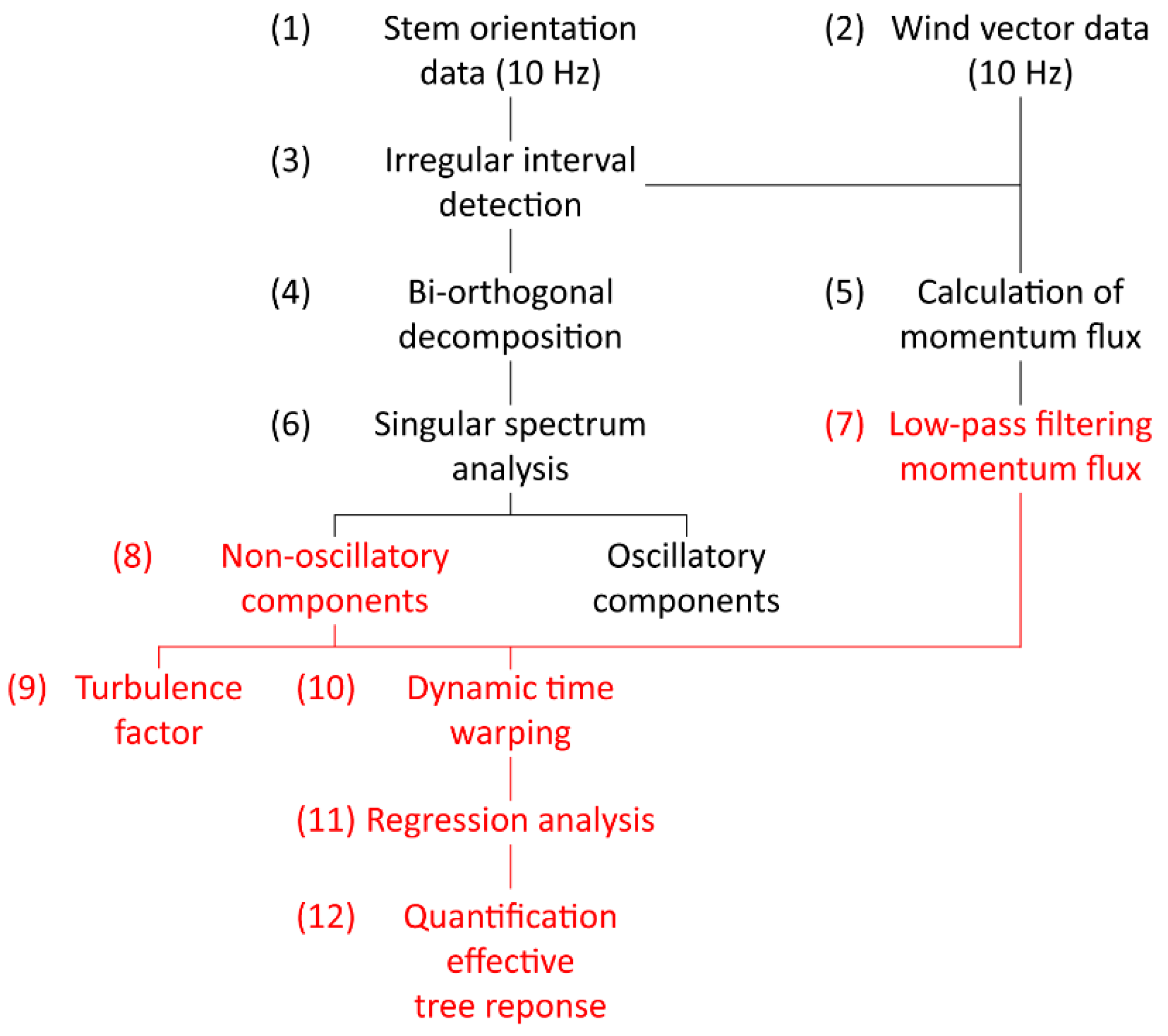
The data collection and analysis of the wind-induced tree response comprised the following main steps (Figure 1): (1) Measurement of orientation (sampling frequency 10 Hz) at seven heights along the stem of the sample tree; (2) measurement of the wind vector (sampling frequency 10 Hz) close to the canopy top; (3) segmentation of orientation time series into irregular intervals; (4) application of the bi-orthogonal decomposition to the orientation time series; (5) calculation and segmentation of momentum flux time series into the irregular intervals found in the orientation time series; (6) application of singular spectrum analysis to separate non-oscillatory from oscillatory orientation components; (7) low-pass filtering of momentum flux time series; (8) separation of non-oscillatory and oscillatory response components; (9) calculation of the turbulence factor; (10) dynamic time warping of non-oscillatory orientation components and low-pass filtered momentum flux; (11) regression of dynamically time warped non-oscillatory orientation components and low-pass filtered momentum flux; (12) quantification of the effective tree response.

2.2. Airflow and Stem Orientation Measurements

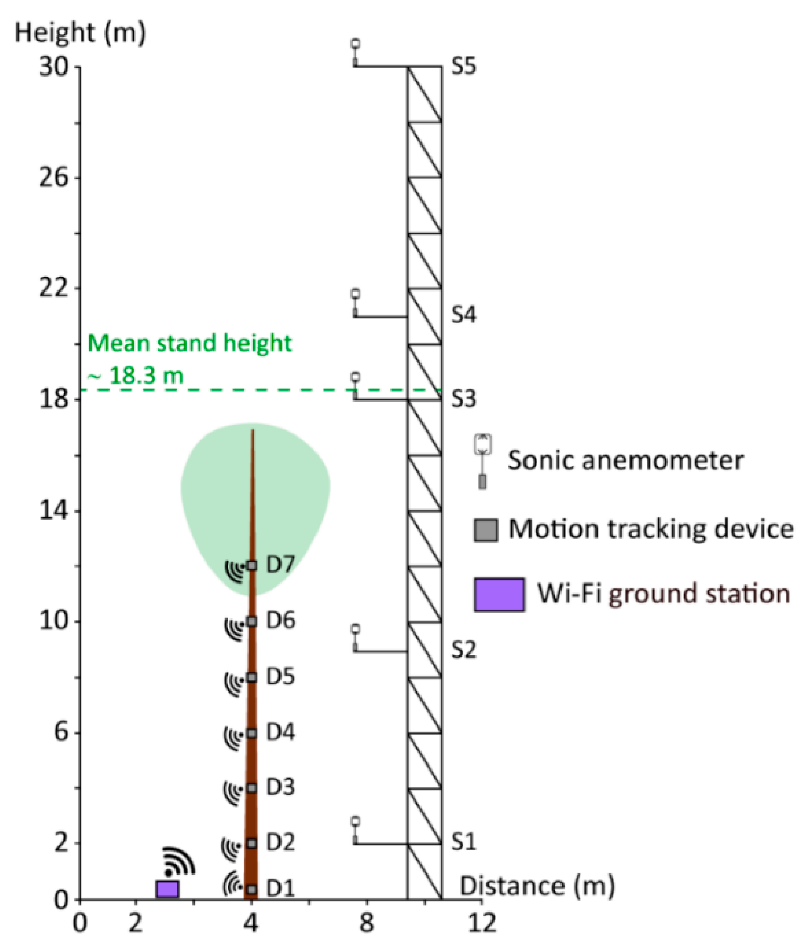
Airflow and stem orientation measurements (sampling frequency 10 Hz) were carried out on 30 January 2019 in a planted Scots pine (Pinus sylvestris L.) forest located in the southern Upper Rhine Valley (47°56′04″ N, 7°36′02″ E, 201 m a.s.l.) in the border area between France and Germany. On that day, wind speed had a pronounced diurnal cycle and 3 s gust speed reached values of 15.0 m/s at the canopy top, which is exceptional for this part of the Upper Rhine Valley. At the time of the measurements, the Scots pine forest at the research site had a mean stand density of 580 trees per hectare and a mean stand height of 18.3 m. The sample tree’s height and its diameter at breast height were 16.8 m and 21.5 cm, respectively. The damped fundamental sway frequency of the stem ($f_0$) was determined at 0.74 Hz using Fourier analysis developed in a previous study [34].

From a vertical profile of five (S1 to S5) ultrasonic anemometers (R.M. Young Company, USA, Type 81000VRE), which were mounted on a 30 m high scaffold tower (Figure 2), data from S3 installed close to canopy top was used to analyze airflow properties. The airflow data from this height was chosen because it allows a close relationship to the dynamics of the tree reactions to be established and the effective wind load components to be estimated [36,37]. The dominant above-canopy wind direction sectors at the research site are south and southwest [47].

The wind-induced, multimodal response of the stem of a Scots pine tree growing at 4.0 m to the southwest of the tower was measured using seven micro electro-mechanical systems (MEMS) motion-tracking devices (MPU-6050^TM Motion Tracking^TM, InvenSense, USA). The motion tracking devices (D1 to D7) are combinations of 3-axis gyroscopes and accelerometers. While the gyroscopes measured the wind-induced rotational motion as angular velocity (°/s), the accelerometer measured the wind-induced acceleration ($g$) along the stem. To monitor the wind-induced response behavior of the stem, D1 to D7 were mounted at heights $h_1$ = 0.1 m, $h_2$ = 2.0 m, $h_3$ = 4.0 m, $h_4$ = 6.0 m, $h_5$ = 8.0 m, $h_6$ = 10.0 m, and $h_7$ = 12.0 m to it. The orientation measurements were carried out at several heights to capture the multimodal vibration behavior of the stem. In an earlier study [34], it was found that the Scots pine trees at the measurement site have at least four measurable modes of vibration.

A Kalman filter implemented in the Sensor Fusion and Tracking Toolbox of Matlab software, version 2019a (The MathWorks, Inc., Natick, MA, USA) was used to calculate stem orientation ($O$) by fusing the signals from the gyroscopes and accelerometers. From the fusion of the signals, information on the offsets of the gyroscopes and accelerometers was obtained and used to calibrate D1 to D7. After sensor fusion, the accuracy of D1 to D7 was tested in the laboratory. In the rest position, it was quantified at ±0.1° up to the 99th percentile. All devices used to measure airflow and stem orientation were pointed northward to define equally aligned coordinate systems. D1 to D7 were installed in white, reflective, 3D-printed housings to minimize unwanted sensor heating and sampled via Wi-Fi.

The total number of points for each of the analyzed time series was 864,000 values (24 h × 36,000 values per hour). As done in previous studies [36,37], the time series measured at $h_1$ to $h_7$ were divided into irregular intervals based on variance changes [48], because the segmentation into irregular intervals allows better representation of short-time wind-tree-interaction dynamics induced by organized turbulence (sweeps and ejections) with dominant periods of 20 s to 40 s at the measurement site. To ensure comparability with previous studies where spectral analysis was used to study the wind-induced tree response behavior, a minimum interval length of 4500 values (≙7:30 min) was defined. This minimum interval length allows a maximum of 192 intervals given equidistant variance changes. However, after the segmentation, the number of measurement device-specific intervals varied between 154 for D5 and 164 for D3 indicating multi-modal response behavior and noise in the stem orientation time series [34,36,37].

2.3. Analysis of Wind-Induced Tree Response

The momentum flux at canopy top ($M$) was used to approximate the wind load acting on the sample tree. As in previous studies [36,37], this approximation was preferred over more sophisticated mechanistic wind load modeling because knowledge on important variables involved in wind-tree-interactions, such as instantaneous changes in the drag coefficient and the frontal area projected to the wind, is still incomplete under real, turbulent canopy wind conditions.

Wind vector data available from S3 was used to calculate $M_{\mathrm{i},\mathrm{j}}$ separately for orientation measured with D1 to D7 as

$$M_{\mathrm{i},\mathrm{j}}=\sqrt{{\left(u_{\mathrm{i},\mathrm{j}}^{’}{w}_{\mathrm{i},\mathrm{j}}^{’}\right)}^2+{\left(v_{\mathrm{i},\mathrm{j}}^{’}{w}_{\mathrm{i},\mathrm{j}}^{’}\right)}^2},$$

(1)

where $u_{\mathrm{i},\mathrm{j}}^{’}$, $v_{\mathrm{i},\mathrm{j}}^{’}$, and $w_{\mathrm{i},\mathrm{j}}^{’}$ are the fluctuations of the horizontal wind vector components $u_{\mathrm{i},\mathrm{j}}$ (east-west), $v_{\mathrm{i},\mathrm{j}}$ (north-south) and the vertical wind vector component $w_{\mathrm{i},\mathrm{j}}$. The fluctuations were calculated by applying the Reynolds decomposition. The subscripts i = 1, …, 7 are indices for D1 to D7 and j is an indicator of the irregular, device-specific intervals.

The wind-induced tree reactions were quantified as orientation vectors ($O_{\mathrm{i},\mathrm{j}}$) whose fluctuations $x_{\mathrm{i},\mathrm{j}}^{’}$ and $y_{\mathrm{i},\mathrm{j}}^{’}$ in the horizontal $x$ (east-west) and $y$ (north-south) directions were calculated according to

$$O_{\mathrm{i},\mathrm{j}}=\sqrt{x_{\mathrm{i},\mathrm{j}}^{’}{}^2+y_{\mathrm{i},\mathrm{j}}^{’}{}^2}.$$

(2)

To highlight central tendencies of the wind-induced tree response, data from the D1- to D7-specific intervals were assigned according to the corresponding mean momentum flux (${\overline{M}}_{\mathrm{i},\mathrm{j}}$) to four (k = 1, …, 4) classes (${\widehat{M}}_{\mathrm{i},1}: {\overline{M}}_{\mathrm{i},\mathrm{j}}$ < 1.0 m²/s², ${\widehat{M}}_{\mathrm{i},2}:$1.0 m²/s² ≤ ${\overline{M}}_{\mathrm{i},\mathrm{j}}$ < 2.0 m²/s², ${\widehat{M}}_{\mathrm{i},3}:$2.0 m²/s² ≤ ${\overline{M}}_{\mathrm{i},\mathrm{j}}$ < 3.0 m²/s² and ${\widehat{M}}_{\mathrm{i},4}: {\overline{M}}_{\mathrm{i},\mathrm{j}}$ ≥ 3.0 m²/s²).

2.4. Bi-Orthogonal Decomposition

From a previous study carried out at the measurement site it is known that the wind-induced response behavior of the Scots pine trees shows at least four vibration modes [34]. Multimodal response behavior requires stem orientation measurements at multiple heights. To quantify the share of common variance in the orientation measurements along the stem, the bi-orthogonal decomposition (BOD) was applied to the stem orientation data. The BOD [49,50] was used to decompose the stem response into a set of seven modes in the time-space domain. To apply the BOD, $O_{1,\mathrm{j}}$ to $O_{7,\mathrm{j}}$ were compiled into one matrix, as described in a previous study [34]. Significant BOD-modes, which explain most of the variance ($VB$) in the wind-induced stem response, were separated from noise using the Kaiser criterion [51]. Ignoring the modes with negligible importance for wind-induced stem motion, the significant modes were then used to reconstruct wind-induced orientation along the stem. Because of the nature of the BOD, the reconstruction led to an adjustment and homogenization of the temporal dynamics in the $O_{\mathrm{i},\mathrm{j}}$ time series.

2.5. Singular Spectrum Analysis

To separate oscillatory ($OS$) from non-oscillatory ($NOS$) sway components in the BOD-adjusted $O_{\mathrm{i},\mathrm{j}}$ time series, the singular spectrum analysis (SSA) was used. The SSA combines embedding of time series with the singular value decomposition [52,53]. In previous studies [35,36], it was demonstrated that the SSA enables the tree-individual separation of fundamental oscillatory sway from a nonlinear trend in the stem response to wind excitation. It was furthermore demonstrated that sway of the Scots pine trees at the measurement site in the fundamental mode, together with the nonlinear trend component, may contain more than 85% of the total SSA-extracted signal variance ($VS$).

Following a previous study [35], the embedding dimension ($L$) was determined by producing trajectory matrices in the range $L$ = 10 to $L$ = 30. The final $L$ value was selected when (1) at least one significant non-oscillatory component could be separated from significant oscillatory components and noise, (2) the difference between the relative variance explained by two of the significant oscillatory components was at a minimum, and (3) the temporal equivalent of $L$ was in the range of ±0.4 s around the damped fundamental sway period of the sample tree stem.

The decomposition of stem motion into $OS$ and $NOS$ is a crucial step in the detection of the tree response components that are effectively coupled with dynamic wind loads [36,37].

2.6. Dynamic Time Warping

Although $M_{\mathrm{i},\mathrm{j}}$ and $O_{\mathrm{i},\mathrm{j}}$ share common features, results from numerous studies demonstrate that the correlation between their temporal dynamics is low [32,35,54,55]. In these studies, values of the corresponding correlation coefficient vary between -0.2 and 0.70. This is due to the nonlinearity of the instantaneous tree response behavior to wind excitation. The nonlinearity is mainly caused by different, concomitant damping processes including aerodynamic damping [56], friction between trees and tree parts [57], multiple mass damping [58], multiple resonance damping [59], damping by branching [59], and viscoelastic damping within above- and below-ground tree parts [60].

To reinforce the instantaneous covariation of wind loading and dynamic tree response (event synchronization), the similarity of $M_{\mathrm{i},\mathrm{j}}$ and $O_{\mathrm{i},\mathrm{j}}$ were quantified using dynamic time warping [61,62]. Dynamic time warping turned $M_{\mathrm{i},\mathrm{j}}$ and $O_{\mathrm{i},\mathrm{j}}$ values into a common linear sequence (warping path) such that the sum of Euclidean distances between corresponding values is smallest and the coincidence between the warped $M_{\mathrm{i},\mathrm{j}}$ and $O_{\mathrm{i},\mathrm{j}}$ sequences is maximized. To align $M_{\mathrm{i},\mathrm{j}}$ and $O_{\mathrm{i},\mathrm{j}}$ sequences, their elements were repeated as often as necessary to highlight their similarities.

If $M_{\mathrm{i},\mathrm{j}}$ and $O_{\mathrm{i},\mathrm{j}}$ have $p$ = 1, …, $P$ and $q$ = 1, …, $Q$ samples, the warping algorithm uses the Euclidean distance $d_{pq}\left(M_{\mathrm{i},\mathrm{j}},O_{\mathrm{i},\mathrm{j}}\right)$ between the $p$th sample of $M_{\mathrm{i},\mathrm{j}}$ and the $q$th sample of $O_{\mathrm{i},\mathrm{j}}$ to stretch $M_{\mathrm{i},\mathrm{j}}$ and $O_{\mathrm{i},\mathrm{j}}$ onto the common linear sequence so that the global signal-to-signal distance measure is at a minimum [63]. The algorithm arranges all possible values of $d_{pq}\left(M_{\mathrm{i},\mathrm{j}},O_{\mathrm{i},\mathrm{j}}\right)$ into a lattice of the form:

$$\begin{gathered} \begin{array}{ccc}\begin{array}{cc}{d}_{1Q}& \begin{array}{cc}{}_{ }& \cdots \end{array}\end{array}& {}_{ }& d_{PQ}\end{array} \\ \begin{array}{ccc}\begin{array}{cc}& \begin{array}{cc}\ddots & {}_{ }\end{array}\end{array}& {}_{ }& \end{array} \\ \begin{array}{ccc}\begin{array}{cc}⋮& \begin{array}{cc}{}_{ }& d_{pq}\end{array}\end{array}& {}_{ }& ⋮\end{array} \\ \begin{array}{ccc}\begin{array}{cc}{d}_{12}& \begin{array}{cc}{d}_{22}& {}_{ }\end{array}\end{array}& \ddots & {}_{ }\end{array} \\ \begin{array}{ccc}\begin{array}{cc}{d}_{11}& \begin{array}{cc}{d}_{21}& \cdots \end{array}\end{array}& {}_{ }& d_{P1}\end{array} \end{gathered}$$

(3)

Then, it searches a path ($d$) through the lattice that is parameterized by the two sequences $ix$ and $iy$ of the same length so that

$$d_{\mathrm{i},\mathrm{j}}={\displaystyle \sum }_{\begin{array}{c}p\in ix\\ q\in iy\end{array}}{d}_{pq}\left(M_{\mathrm{i},\mathrm{j}},O_{\mathrm{i},\mathrm{j}}\right)$$

(4)

is at a minimum. The algorithm starts at $d_{11}\left(M_{\mathrm{i},\mathrm{j}},O_{\mathrm{i},\mathrm{j}}\right)$ and ends at $d_{PQ}\left(M_{\mathrm{i},\mathrm{j}},O_{\mathrm{i},\mathrm{j}}\right)$. The changes of the warping path are used to find the minimum distance between $M_{\mathrm{i},\mathrm{j}}$ and $O_{\mathrm{i},\mathrm{j}}$ are combinations of vertical (($p$,$q$) → ($p$ + 1,$q$)), horizontal (($p$,$q$) → ($p$,$q$ + 1)), and diagonal moves (($p$,$q$) → ($p$ + 1,$q$ + 1)).

The Signal Processing Toolbox of the Matlab software, version 2019a (The MathWorks, Inc., Natick, Massachusetts) was used to dynamically warp $M_{\mathrm{i},\mathrm{j}}$ and $O_{\mathrm{i},\mathrm{j}}$.

2.7. Turbulence Factor Calculation

To compare the impact of maximum effective dynamic wind loading to the impact of median wind loading on the effective tree response, the turbulence factor ($T$) was calculated as

$$T_{\mathrm{i},\mathrm{j}}=\frac{NO{S}_{{98}_{\mathrm{i},\mathrm{j}}}}{NO{S}_{{50}_{\mathrm{i},\mathrm{j}}}},$$

(5)

with $NO{S}_{{98}_{\mathrm{i},\mathrm{j}}}$ being the measuring height- and interval-specific 98th percentile of $NOS$ that approximates the maximum wind load; $NO{S}_{{50}_{\mathrm{i},\mathrm{j}}}$ is the median measuring height- and interval-specific wind load representing central tendencies in the effective wind excitation of the sample tree.

The gust factor $G$, which was based on maximum 3 s gust speed in earlier studies [64,65], was not used and evaluated here, because it cannot be calculated because of the kind of data processing in this study.

3. Results and Discussion

3.1. Mean Momentum Flux-Induced Tree Response

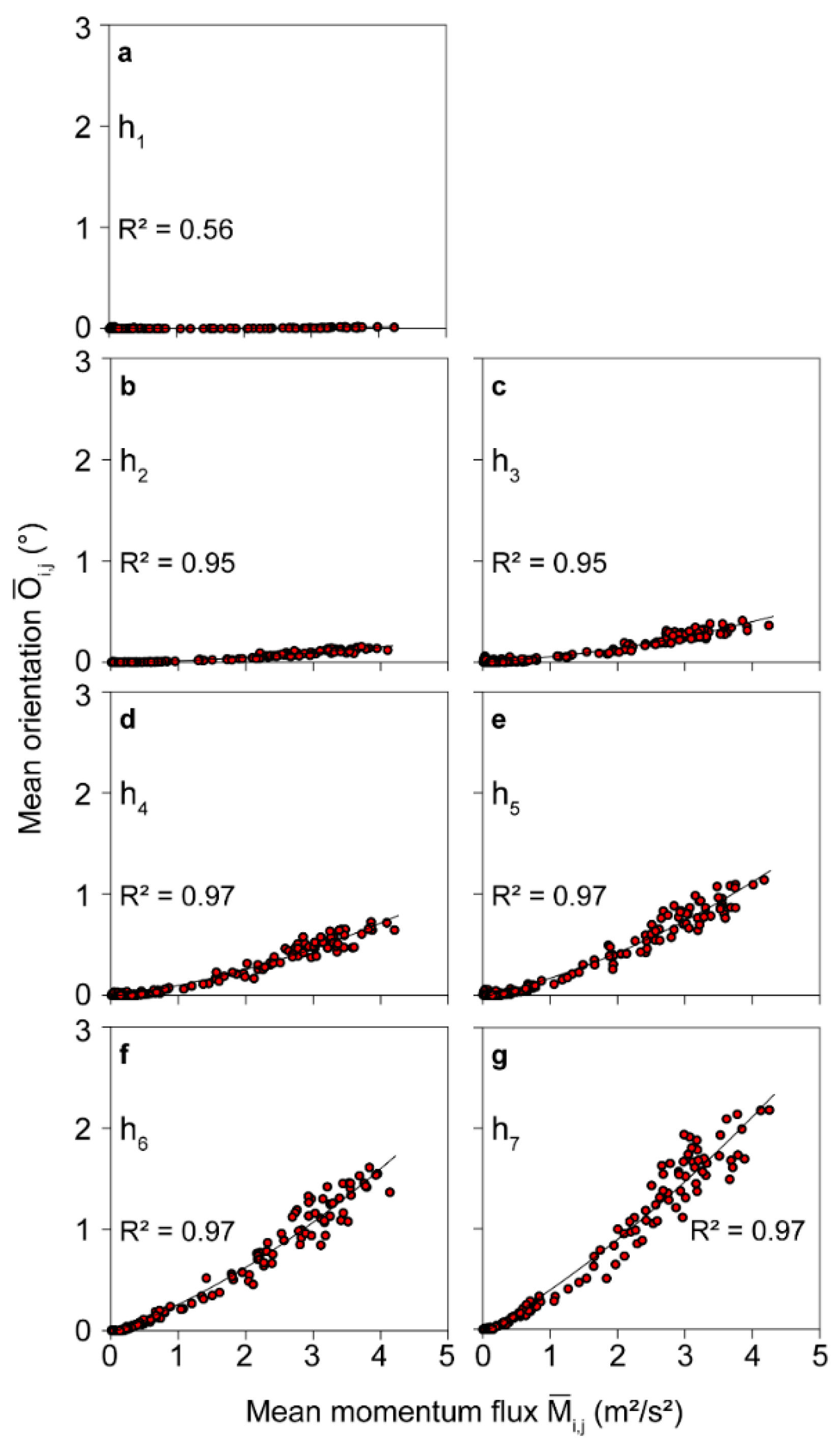
The ${\overline{M}}_{\mathrm{i},\mathrm{j}}$-dependent mean orientation at $h_1$ to $h_7$ is displayed in Figure 3. At the stem base, ${\overline{O}}_{1,\mathrm{j}}$ is close to zero over the entire ${\overline{M}}_{1,\mathrm{j}}$ range. With increasing measuring height, ${\overline{O}}_{\mathrm{i},\mathrm{j}}$ increases along the stem toward the crown reaching maximum ${\overline{O}}_{7,\mathrm{j}}$ values of 2.2°. To quantify the statistical dependence between ${\overline{M}}_{\mathrm{i}}$ and ${\overline{O}}_{\mathrm{i}}$, second order polynomials were fitted by the least squares approach. The resulting coefficients of determination ($R^2$) are very high at $h_2$ to $h_7$ and vary in the range 0.95 to 0.97. The marginal variation of $R^2$ from $h_2$ to $h_7$ may result from the multimodal response behavior of the stem to wind loading. A much lower $R^2$ value was calculated from the orientation measurements made at $h_1$. As will be confirmed later, the low $R^2$ value at the stem base results from very weak wind excitation of the stem part closest to the ground.

The use of irregular intervals led to higher $R^2$ values compared to intervals of equal length. The differences between irregular and fixed-length 10 min intervals were assessed by the difference in $R^2$ ($\Delta R^2$). The largest $\Delta R^2$ value was quantified at $h_1$ being $\Delta R^2$ = 0.38. At $h_2$, $\Delta R^2$ = 0.06; at $h_3$, $\Delta R^2$ = 0.04. Higher up, at $h_4$ to $h_7$, $\Delta R^2$ decreased further to 0.02. The larger differences in $R^2$ in the lower parts of the stem are because the wind loads caused a weaker response than in higher parts of the stem. In the lower parts of the stem, only the highest wind loads were able to excite a distinct response. Thus, it can be concluded that the importance of the selection of irregular intervals shows a dependence on the impact of wind loading in different parts of the stem.

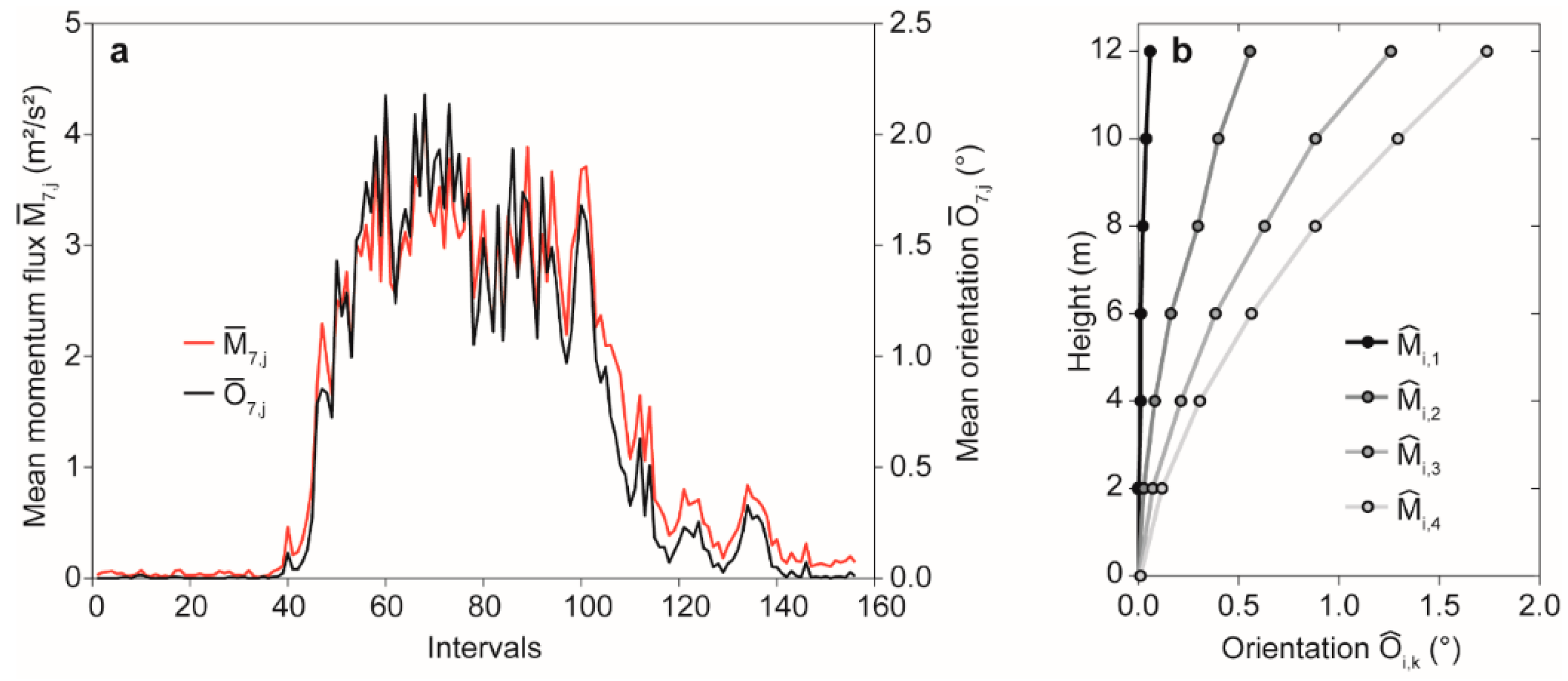
The corresponding temporal behavior of ${\overline{M}}_{7,\mathrm{j}}$ and ${\overline{O}}_{7,\mathrm{j}}$ is shown Figure 4a. From this, it is clear that ${\overline{O}}_{7,\mathrm{j}}$ closely follows ${\overline{M}}_{7,\mathrm{j}}$ over the course of the analyzed day. The ${\widehat{M}}_{\mathrm{k}}$-related tree response shows increasing mean deflection at $h_1$ to $h_7$ with increasing wind load (Figure 4b). At low wind loading in ${\widehat{M}}_{\mathrm{i},1}$, the entire stem is only slightly deflected. In this momentum flux class, the orientation values mostly varied in the range of the measurement uncertainty. For ${\widehat{M}}_{7,4}$, ${\widehat{O}}_{7,4}$ = 1.7° at $h_7$ = 12 m.

3.2. Bi-Orthogonal Decomposition

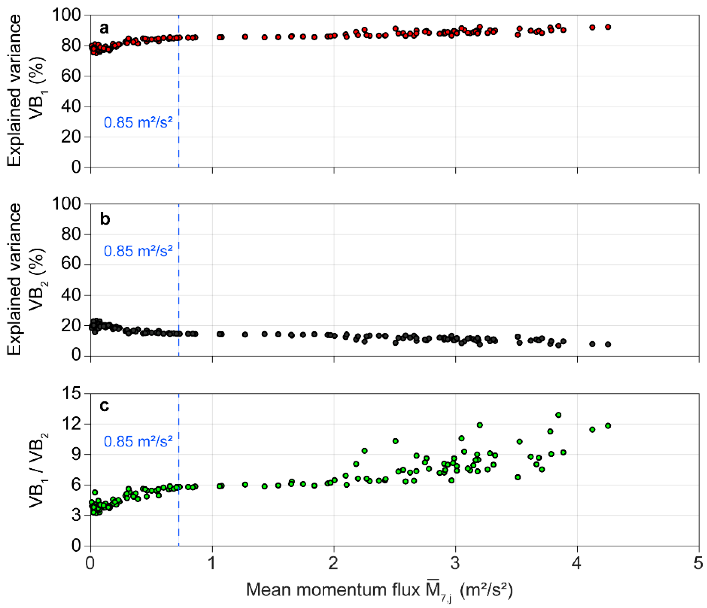
As can be expected from a previous study into plantation-grown Scots pine [34], results from the BOD demonstrate that orientation measurements at $h_1$ to $h_7$ strongly covary. The largest part of the variance in the interval-specific orientation matrices was assigned to the first BOD component with $V{B}_1$ varying between 75 and 93% as a function of ${\overline{M}}_{7,\mathrm{j}}$ (Figure 5a). Much less of the variance in the orientation matrix was explained by the second BOD component, with $V{B}_2$ values ranging wind, load-dependent, from 7 to 23% (Figure 5b). In addition, it becomes clear that $V{B}_1$ increases with increasing wind load while $V{B}_2$ decreases as the wind load increases. The opposing tendencies in the behavior of $V{B}_1$ and $V{B}_2$ become particularly evident when their ratio ($V{B}_1/V{B}_2$) is calculated (Figure 5c). Whereas at the lowest wind loads $V{B}_1/V{B}_2$ ≈ 4, its value increases at least to 8 for the highest wind loads. The remaining variance in the orientation matrices, which was assigned to BOD components 3 to 7, ranged between 0 and 2%.

When ${\overline{M}}_{7,\mathrm{j}}$ > 0.85 m²/s², the first component was the only significant BOD component. In all intervals where ${\overline{M}}_{7,\mathrm{j}}$ ≤ 0.85 m²/s², two significant BOD components were detected. The presence of only one significant BOD component, even at very low wind loads, indicates that the kinetic energy transferred to the tree was mostly converted into elastic energy that drove the sway of the stem in one mode. Small amounts of kinetic energy contained in the airflow at canopy top were enough to induce movement in the stem down to $h_2$. Damping processes such as multiple mass damping in the crown and friction with neighboring trees that can be assigned to the second BOD component [34], were only of minor importance for overall tree motion damping.

3.3. Singular Spectrum Analysis

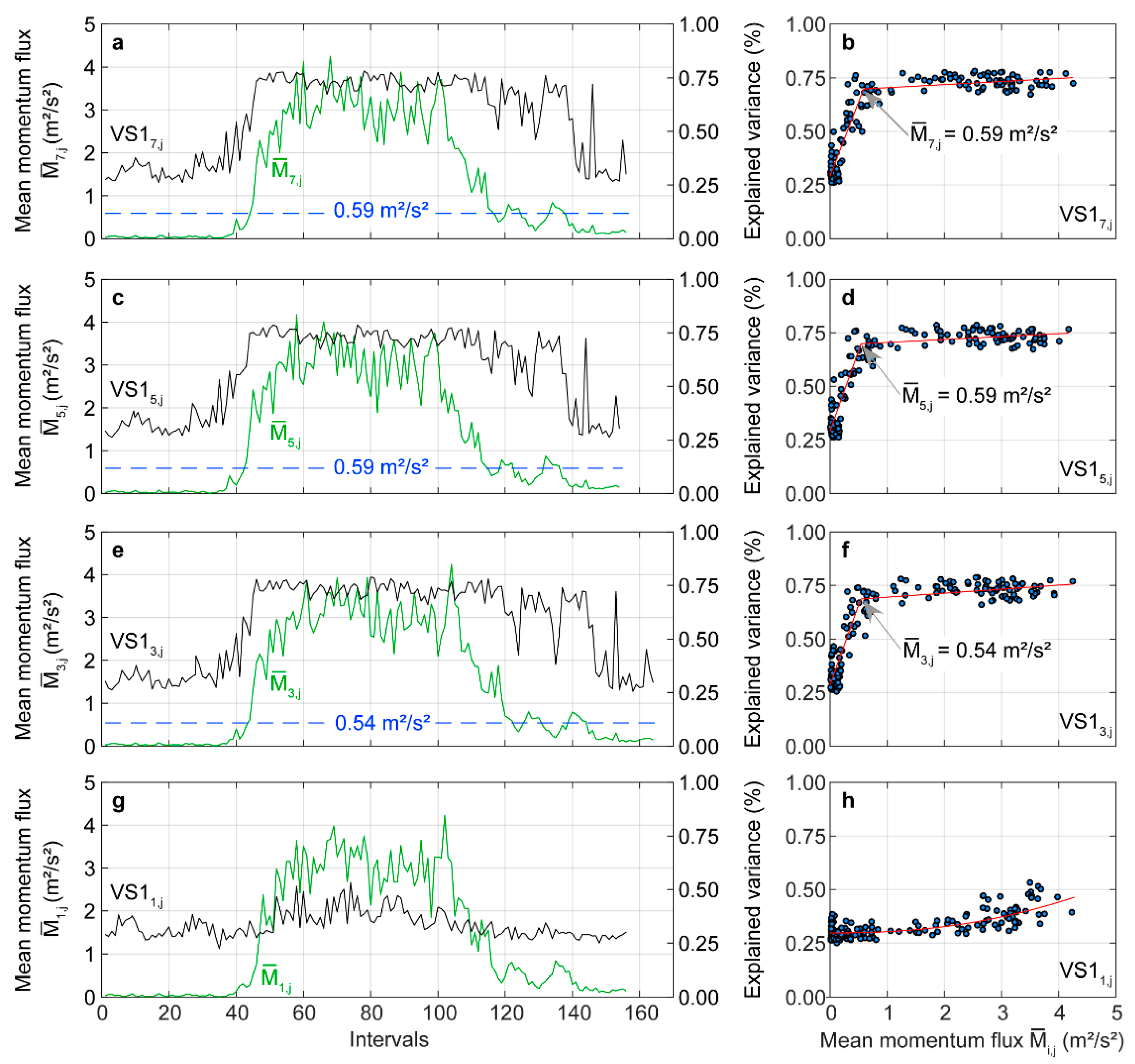
Except for the stem base, the wind-induced stem motion was dominated by $NO{S}_{\mathrm{i},\mathrm{j}}$. As examples, the temporal evolution of $V{S}_{\mathrm{i},\mathrm{j}}$ associated with $NO{S}_{\mathrm{i},\mathrm{j}}$ ($VS{1}_{\mathrm{i},\mathrm{j}}$) over the course of the analyzed day is shown in Figure 6 for $M_{\mathrm{i},\mathrm{j}}$ at $h_7$, $h_5$, $h_3,$ and $h_1$. From the $VS{1}_{7,\mathrm{j}}$, $VS{1}_{5,\mathrm{j}}$, and $VS{1}_{3,\mathrm{j}}$ curves illustrated in Figure 6a,c,e, respectively, it can be deduced that the importance of $NO{S}_{\mathrm{i},\mathrm{j}}$ to wind excitation in the upper stem parts grows with increasing wind load, a behavior similar to the behavior reported in a previous study [36]. In intervals, where only very weak wind loading of less than 0.59 m²/s² occurs, $VS{1}_{7,\mathrm{j}}$ is about 25%, with ${\overline{M}}_{7,\mathrm{j}}$ = 0.59 m²/s² being the estimated change point from a two-phase regression model [66]. The change point clearly indicates the change in the tree response behavior to wind excitation. The change points are also drawn as dashed blue lines in Figure 6a,c,e to emphasize once again that the tree response behavior to wind loading is very quickly dominated by sway in the non-oscillatory SSA mode after the blue line has been crossed. At higher wind loads, $VS{1}_{7,\mathrm{j}}$, $VS{1}_{5,\mathrm{j}},$ and $VS{1}_{3,\mathrm{j}}$ steeply increase and reach values up to 75%. This increase documents the rapid and strong growth of the importance of $NO{S}_{\mathrm{i},\mathrm{j}}$ for the total tree response in the upper parts of the stem.

In contrast to the other stem sections, $VS{1}_{1,\mathrm{j}}$ changed to a lesser extent during the day (Figure 6g). It fluctuated between 25% and 50% with a much weaker dependence on ${\overline{M}}_{1,\mathrm{j}}$. Therefore, a two-phase regression model could not be fitted to the point cloud shown in Figure 6h. Instead, the red curve is the result from fitting a second order polynomial model to the $VS{1}_{1,\mathrm{j}}$ point cloud. However, there is an increasing tendency in $VS{1}_{1,\mathrm{j}}$ with increasing wind load.

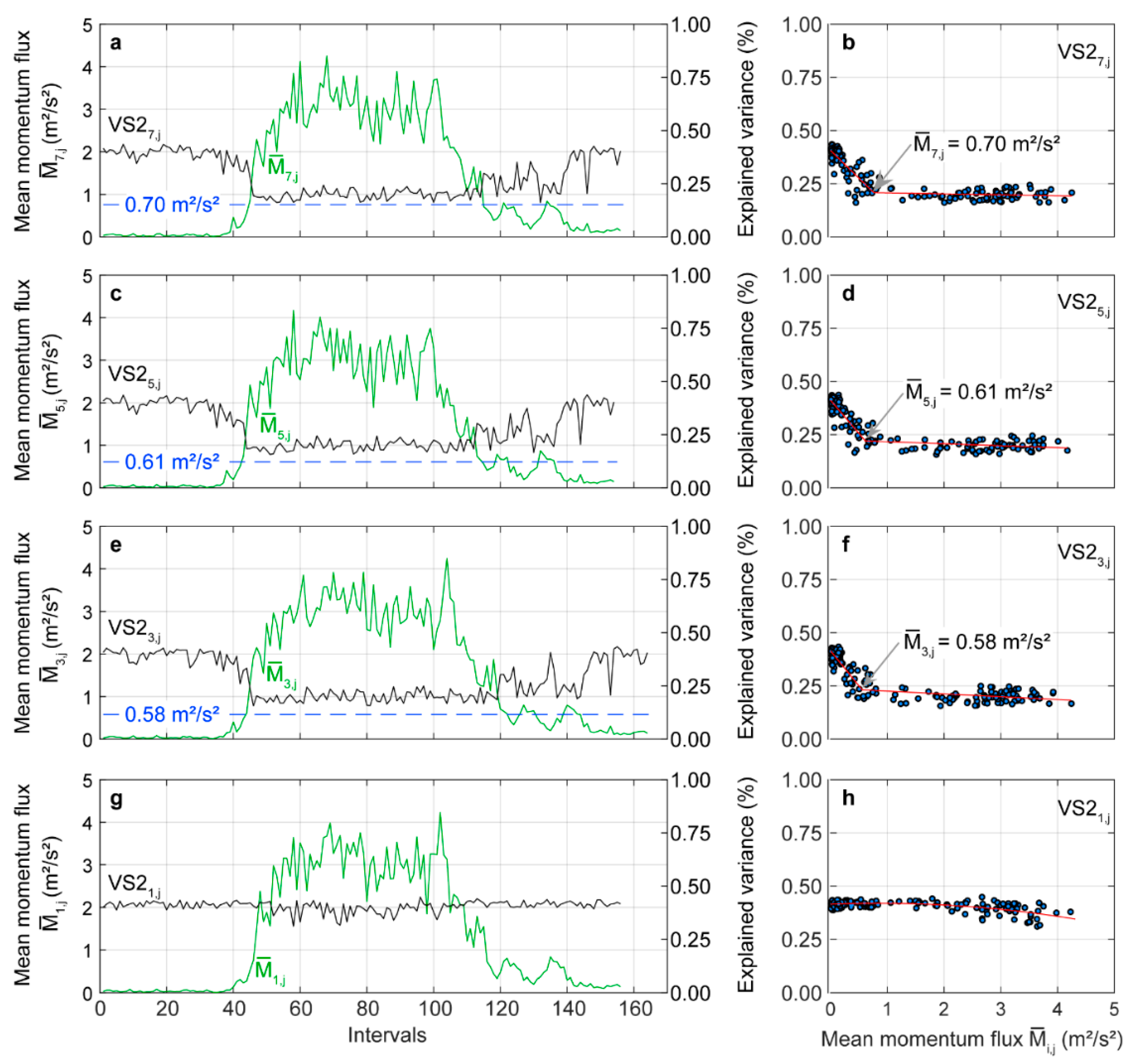
An opposite pattern to $VS{1}_{\mathrm{i},\mathrm{j}}$ is found in the variance explained by $O{S}_{\mathrm{i},\mathrm{j}}$ ($VS{2}_{\mathrm{i},\mathrm{j}}$). At low wind loading of ${\overline{M}}_{7,\mathrm{j}}$ < 0.70 m²/s², more than 20% of the variance contained in the $O_{7,\mathrm{j}}$ time series was assigned to stem motion in the fundamental mode (Figure 7a). With increasing wind load, $VS{2}_{7,\mathrm{j}}$ rapidly drops to just over 10%. Again, the value of ${\overline{M}}_{7,\mathrm{j}}$ < 0.70 m²/s², where the distribution of signal energy on the response components changes, corresponds to the change point of the results from a two-phase regression model (Figure 7b). The dashed blue line in Figure 7a reinforces the impression on the wind load-dependent drop of $VS{2}_{7,\mathrm{j}}$ further. Similar changes as in $VS{2}_{7,\mathrm{j}}$ can also be found in $VS{2}_{5,\mathrm{j}}$ (Figure 7c) and $VS{2}_{3,\mathrm{j}}$ (Figure 7e). At the stem base, $VS{2}_{1,\mathrm{j}}$ is almost independent of ${\overline{M}}_{1,\mathrm{j}}$ (Figure 7g). It varies at about 40% over the course of the day with decreasing tendency at higher wind loading.

The change point values associated with the wind load-dependent drop of $VS{2}_{\mathrm{i},\mathrm{j}}$ are in the same wind loading range as the change point values of $VS{1}_{\mathrm{i},\mathrm{j}}$. This is a clear indication that the importance of $O{S}_{\mathrm{i},\mathrm{j}}$ in the fundamental mode for the total wind-induced motion decreases whereas $NO{S}_{\mathrm{i},\mathrm{j}}$ gains considerably in importance with increasing wind load. Moreover, it can be ruled out that wind-induced resonance boosted tree motion. These findings are in line with results from previous studies [36,37,67] and have important implications for the interpretation of wind-induced tree sway in the fundamental mode. Since sway in the fundamental mode is largely decoupled from the canopy airflow, it is an efficient way to dissipate kinetic energy that was transferred from the airflow into tree motion [59].

Although upper stem parts reacted strongly to the wind excitation, the wind loads were not strong enough to cause pronounced reactions at the stem base. Therefore, it is assumed that the anchoring of the tree in the ground was sufficient and that there was no acute risk of the tree being damaged by the wind.

The increasing importance of $NO{S}_{\mathrm{i},\mathrm{j}}$ in dependence of the wind load has implications for the significance of the dynamic excitation in the estimation of storm stability by static tree pulling tests. It is very likely that sway in the fundamental mode does not severely affect the tree resistance against wind loading. In addition to the quasi-static wind load, it is the occurrence of exceptionally strong organized turbulence structures such as sweeps or ejections to which forest trees respond that cause damage [68].

3.4. Dynamic Time Warping

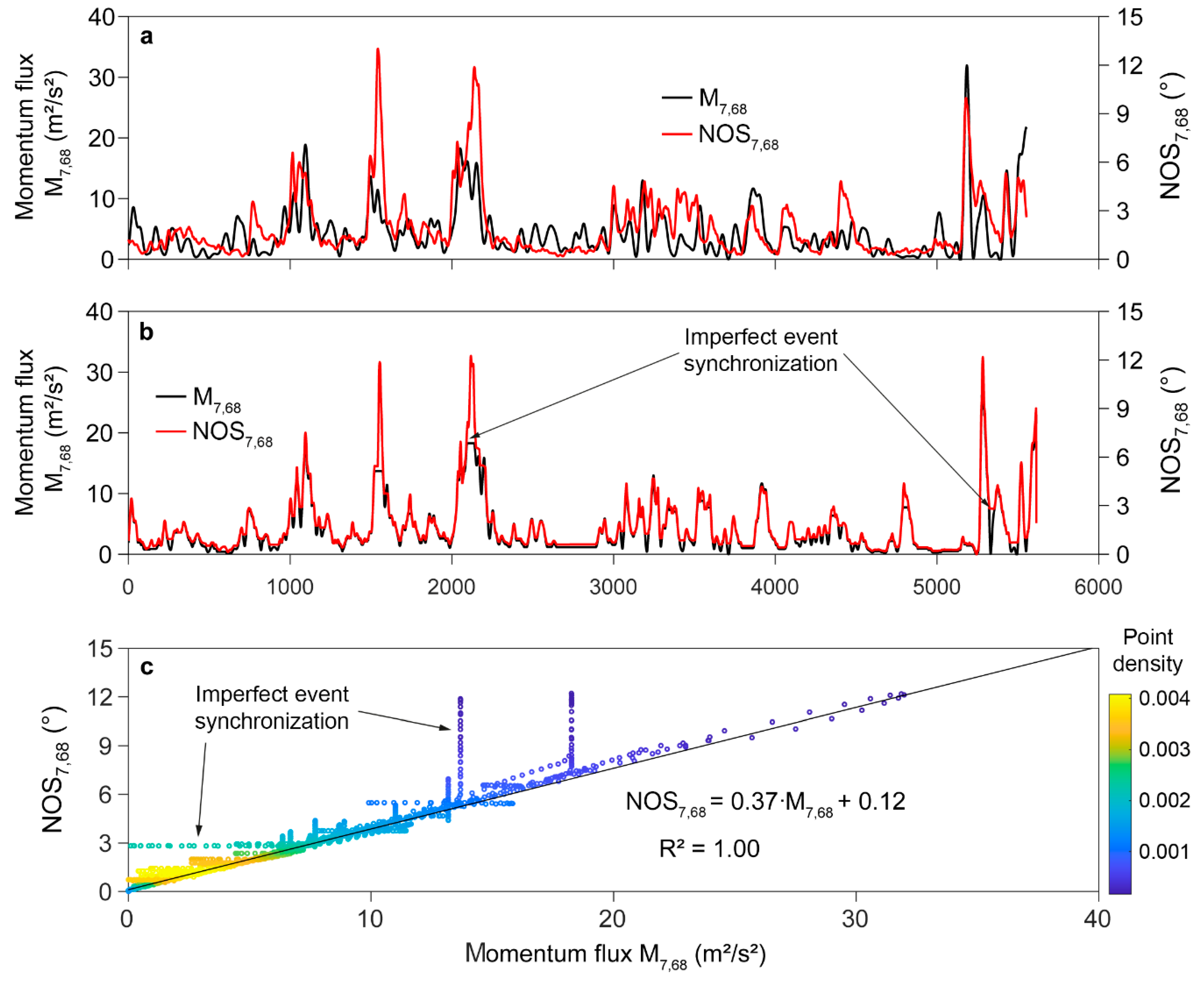
Based on the findings from SSA, further analysis was focused on the non-oscillatory tree response component. Since it has been demonstrated that this component is most strongly coupled with components in $M_{\mathrm{i},\mathrm{j}}$ consisting only of frequencies below $f_0$ [36,37], $M_{\mathrm{i},\mathrm{j}}$ time series were low-pass filtered using a cut-off frequency of 0.2 Hz. The applied fourth order Butterworth filter attenuated all variations of $M_{\mathrm{i},\mathrm{j}}$ shorter than 5.0 s. Figure 8 shows an example of low-pass filtered momentum flux and $NO{S}_{7,68}$. In the presented 68th interval with an original length of 5553 values, maximum low-pass filtered $M_{7,68}$ values exceeded 31 m²/s² and $NO{S}_{7,68}$ reached values of 12° (Figure 8a). It is evident that the temporal variation of $NO{S}_{7,68}$ does not always match the temporal variation of low-pass filtered $M_{7,68}$ although there are only a few meters distance between the sample tree and the airflow measurement at the canopy top.

After the feature alignment by dynamic time warping that synchronizes all strong wind load events with the highest $NO{S}_{7,68}$ values, the interval length increased to 9309 values. To enable the comparison to the original time series, time warped $M_{7,68}$ and $NO{S}_{7,68}$ were downsampled to the original interval length. Although the dynamic time warping considerably modifies low-pass filtered $M_{7,68}$ and $NO{S}_{7,68}$, it cannot achieve a perfect match of the temporal dynamics in the two time series (Figure 8b). However, the alignment significantly improves their coincidence. More importantly, the approach includes all dynamic and quasi-static wind load components that effectively deflect the stem of the sample tree. A scatter plot of the aligned $M_{7,68}$ and $NO{S}_{7,68}$ time series (Figure 8c), can visualize this. Most of the values are tightly grouped along the regression line. The highest $NO{S}_{7,68}$ point density occurs at the lowest $M_{7,68}$ values.

The values from the time series segments in which the adjustments are not optimal appear as arrays of column- and bar-like constant values (less than 10% of the total number of values) because they are filled up with constant values. Ignoring these values, the robust fitting (with 95% confidence bounds) of the points yields $R^2$ = 1.00, which stands for an excellent fit. The slope of the regression line ($Sl$) indicates the rate of change in $NO{S}_{7,68}$ (0.37°/(m²/s²)) in dependence of low-pass filtered $M_{7,68}$.

The high $R^2$ values obtained in this study are well in the range of $R^2$ values (0.79–0.97) reported in previous studies where interval maxima of tree response were compared to interval maxima of wind speed [69] and wind speed squared [26]. On the other hand, the calculation of $R^2$ of the relationship between hourly maximum tree response and the square of the hourly canopy-top wind speed as described in a previous study [26], yielded values between $R^2$ = 0.51 at $h_1$ to $R^2$ = 0.84 at $h_6$ which is also in the range of $R^2$ values reported in [26] but clearly lower than the $R^2$ values obtained using the approach proposed in this study.

The dynamic time warping resulted in a strong linear dependence of $NO{S}_{7,68}$ on low-pass filtered $M_{7,68}$ over the entire $NO{S}_{7,68}$ range. Because of this dependence, the impact of effective dynamic and quasi-static wind loading on tree deflection can be directly estimated. Compared to static tree pulling tests and maximum tree response vs. maximum wind speed approaches, this kind of response assessment incorporates all turbulent and quasi-static components effectively involved in the occurrence of the maximum wind-induced tree response.

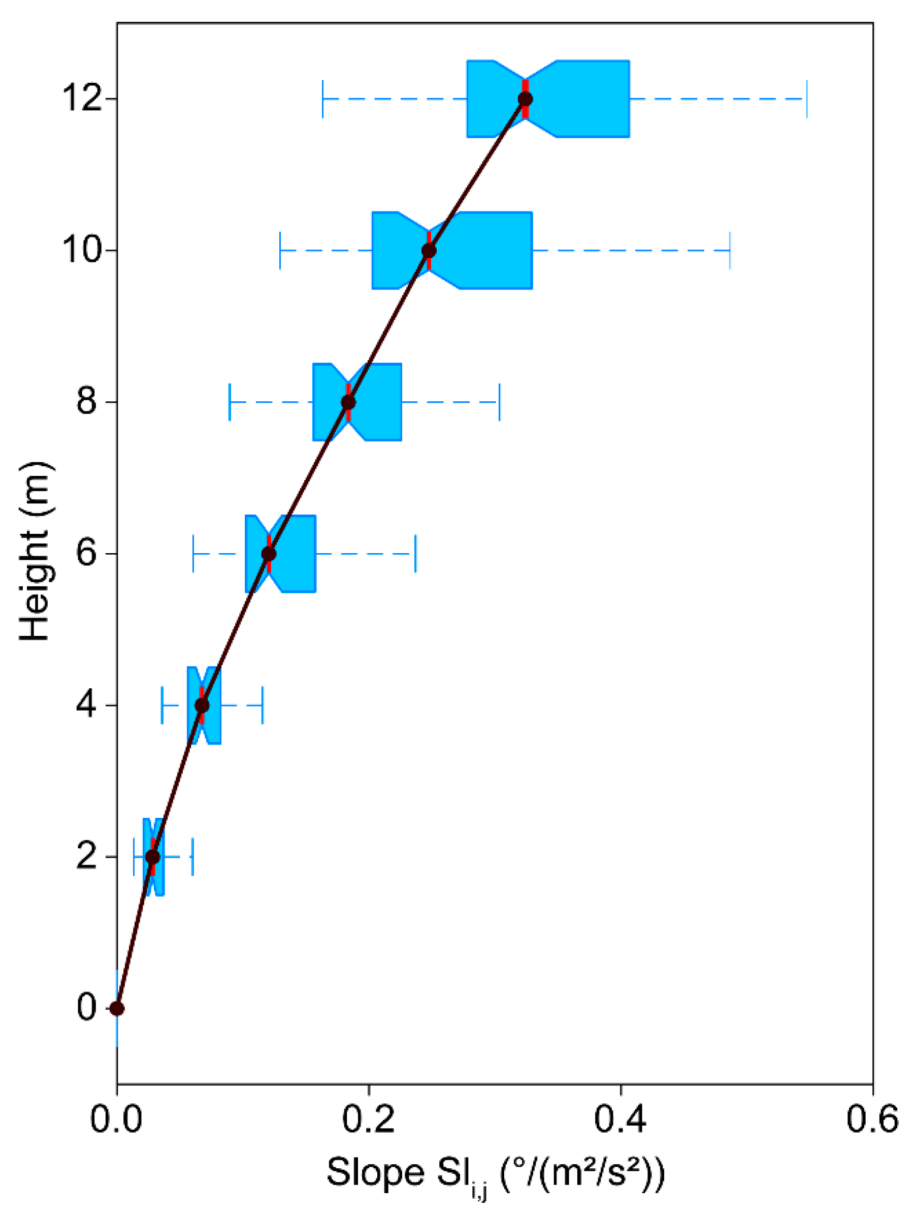
A summary of all $S{l}_{\mathrm{i},\mathrm{j}}$ values calculated from linear regression analysis between low-pass filtered $M_{\mathrm{i},\mathrm{j}}$ and $NO{S}_{\mathrm{i},\mathrm{j}}$ is presented in Figure 9 by boxplots. Median slope values as indicated by a red vertical line, increase from 0.00 °/(m²/s²) at $h_1$ to 0.32 °/(m²/s²) at $h_7$. In the upper parts of the trunk, the dispersion of the $S{l}_{\mathrm{i},\mathrm{j}}$-values also increases, which expresses the range of possible stem reactions to the effective wind loads. In contrast to previous approaches, this type of analysis provides probabilistic estimates of the wind load-dependent effective tree response instead of providing fixed $Sl$ values.

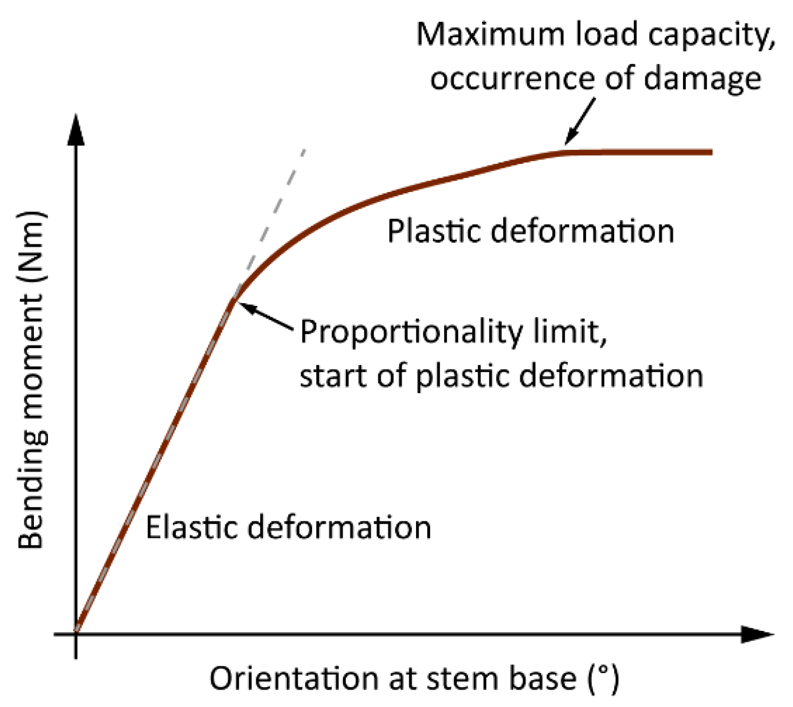
Since ${\overline{O}}_{1,\mathrm{j}}$ was always very close to zero and did not increase after the impact of the highest wind loads, it is assumed that the root plate resisted all wind loads. In the previous quasi-static tree pulling studies [27,28], root plate inclination less than a benchmark of 0.25° was considered to be sufficiently low to stay in the elastic deformation range below the limit of proportionality in stem bending (Figure 10) and to prevent primary failure in the roots. If this benchmark is transferred to this study, one can assume that the tree response at the stem base was always in the range of elastic deformation and did not cause any plastic deformation in the roots.

Although this study allows only limited portability using only one plantation-grown Scots pine tree, there is a great potential to transfer the described approach to more complex structured trees. Previous studies have already shown for other trees and other tree species that non-oscillatory tree response strongly depends on the effective wind loading [34,35,36,38,39]. However, for now the results can only be interpreted over the range of non-destructive wind loading.

3.5. Turbulence Factor

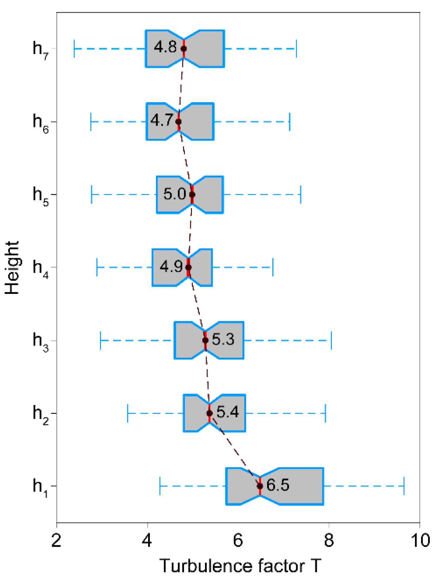
Boxplots depict the variation of $T_{\mathrm{i},\mathrm{j}}$ along the stem in all intervals, where low-pass filtered ${\overline{M}}_{\mathrm{i},\mathrm{j}}$ > 1.0 m²/s² (Figure 11). The median of $T_{1,\mathrm{j}}$ = 6.5 is significantly (95% confidence) higher than at all other heights. The medians of $T_{2,\mathrm{j}}$ = 5.4 to $T_{7,\mathrm{j}}$ = 4.8 vary in a narrow range with no significant differences as indicated by the overlap of the notches in the boxes. That $T_{\mathrm{i},\mathrm{j}}$ is not a constant value can be deduced from the displayed interquartile ranges. At $h_1$, $T_{1,\mathrm{j}}$ shows the greatest variability. There, it varies by 2.1 between $T_{1,\mathrm{j}}$ = 5.8 and $T_{1,\mathrm{j}}$ = 7.9. From $h_2$ to $h_7$, the interquartile ranges span 1.3 to 1.7. Since $T_{\mathrm{i},\mathrm{j}}$ is not a constant along the stem and is dependent on the wind load, it would therefore not be appropriate to use $T_{\mathrm{i},\mathrm{j}}$ as a fixed value in systems for storm damage analysis, but to implement it probabilistically.

The significantly higher median $T_{1,\mathrm{j}}$ value at stem base may be explained by the strength of the effective wind load. It was sufficient to excite the upper part of the stem in a similar way, but mostly too low to stimulate stem reactions at $h_1$. Only the highest wind loads were able to excite a pronounced response at the stem base. This implies that the height, at which the turbulence factor, the gust factor and the turning moment coefficient are quantified as a function of the wind load, affects their value, and thus also the assessment of the storm hazard.

The comparison of the $T_{\mathrm{i},\mathrm{j}}$ values determined here shows that they deviate from the gust factors reported in previous papers [64,65]. These papers report both lower and higher gust factors from field and wind tunnel experiments. Thus, it can be concluded that there is still great uncertainty in the quantification of the impacts of maximum and quasi-static wind loading on the tree response. These differences are certainly largely due to the different approaches chosen in the studies. One advantage of the approach applied here is that only effective wind loads and tree response components were considered and not the entire range of wind loads and response components, which includes ineffective components such as oscillatory sway in the fundamental mode. We therefore argue that the consideration of oscillatory components leads to biased relationships between response maxima and wind maxima.

4. Conclusions

In contrast to previous approaches, the proposed method uses only effective wind loads to quantify wind-induced reactions of the sample tree. It excludes sway at the damped fundamental frequency that is only to a small extent directly caused by wind loads. The linearization of the relationship between effective wind loading and non-oscillatory tree response allows the direct quantification of the resistance of the tree to wind-induced deflection. Separating effective from ineffective wind loading improves the estimation of the impact of maximum loads from turbulence under high wind conditions. Under high wind loads, the separation is particularly important and necessary because trees are exposed to a preload, which is caused by the quasi-static load associated with high mean wind speed. We argue that the combined assessment of the impacts of high quasi-static wind loads and high dynamic wind loads improves the of quantification of the damage probability. This is because the proposed method can be used to localize the limits of elastic stem deformation by extrapolating the observed linear relationships of effective wind-tree coupling. Because of the expected changes in the dependence of the tree response on wind loading in the range of plastic deformation until tree failure, the method is certainly capable of better delimiting the plastic deformation range. The proposed approach also enables probabilistic estimates of the wind load-dependent tree response to effective wind loading using slope values of the regression calculated from low-pass filtered momentum flux at canopy top and non-oscillatory SSA components instead of using absolute tree response measures that are very likely to fluctuate under real conditions.

Since the sampled Scots pine is a simply structured tree whose wind-induced response is clearly dominated by vibrations of the stem in the first mode, it is to be expected that there are not only differences in the parameterization of the observed linear relationships specific to different trees and tree species, but also differences caused by stand structure and site diversity. Therefore, further work needs to be carried out to determine these relationships for many more trees in order to prepare their implementation in existing systems used for storm damage analysis. With the implementation in these systems, the effective impact of wind load on trees can be better estimated and thus improve the estimation of critical wind speeds. Further investigations must also be carried out regarding the comparability between the proposed method and tree pulling tests. Since this study has shown that the quasi-static, and not the dynamic tree reaction in the range of the fundamental sway frequency dominates the maximum wind-induced response of the sample tree, there is certainly a great potential for connecting the results from both approaches in future studies on wind damage to trees.

References

- Gardiner, B.; Blennow, K.; Carnus, J.-M.; Fleischer, P.; Ingemarson, F.; Landmann, G.; Lindner, M.; Marzano, M.; Nicoll, B.; Orazio, C.; et al. Destructive storms in European forests: Past and forthcoming impacts. Available online: https://ec.europa.eu/environment/forests/pdf/STORMS%20Final_Report.pdf (accessed on 19 June 2019).
- Gregow, H.; Laaksonen, A.; Alper, M.E. Increasing large scale windstorm damage in Western, Central and Northern European forests, 1951–2010. Sci. Rep. 2017, 7, 46397. [Google Scholar] [CrossRef] [PubMed] [Green Version]
- Jung, C.; Schindler, D. Historical winter storm atlas for Germany (GeWiSA). Atmosphere 2019, 10, 387. [Google Scholar] [CrossRef] [Green Version]
- Schelhaas, M.-J.; Nabuurs, G.-J.; Schuck, A. Natural disturbances in the European forests in the 19th and 20th centuries. Glob. Change Biol. 2003, 9, 1620–1633. [Google Scholar] [CrossRef]
- Gardiner, B.; Schuck, A.; Schelhaas, M.-J.; Orazio, C.; Blennow, K.; Nicoll, B. What Science Can Tell Us. In Living with Storm Damage to Forests; European Forest Institute: Barcelona, Spain, 2013. [Google Scholar]
- Mayer, H.; Schindler, D. Forest meteorological fundamentals of storm damage in forests in connection with the extreme storm “Lothar”. Allg. Forst Jgdztg. 2002, 173, 200–208. [Google Scholar]
- Lindroth, A.; Lagergren, F.; Grelle, A.; Klemendtsson, L.; Langvall, O.; Weslien, P.; Tuulik, J. Storms can cause Europe-wide reduction in forest carbon sink. Glob. Chang. Biol. 2009, 15, 346–355. [Google Scholar] [CrossRef]
- Dahle, A.G.; James, K.R.; Kane, B.; Grabosky, J.C.; Detter, A. A review of factors that affect the static load-bearing capacity of urban trees. Arboricul. Urban. For. 2017, 43, 89–106. [Google Scholar]
- Gardiner, B.; Byrne, K.; Hale, S.; Kamimura, S.; Mitchell, S.J.; Peltola, H.; Ruel, J.-C. A review of mechanistic modelling of wind damage risk to forests. Forestry 2008, 81, 447–463. [Google Scholar] [CrossRef] [Green Version]
- Peltola, H.; Kellomäki, S.; Vaisanen, H.; Ikonen, V.-P. A mechanistic model for assessing the risk of wind and snow damage to single trees and stands of Scots pine, Norway spruce, and birch. Can. J. For. Res. 1999, 29, 647–661. [Google Scholar] [CrossRef]
- Gardiner, B.; Peltola, H.; Kellomäki, S. Comparison of two models for predicting the critical winds required to damage coniferous trees. Ecol. Model. 2000, 129, 1–23. [Google Scholar] [CrossRef]
- Ancelin, P.; Courbaud, B.; Fourcaud, T. Development of an individual tree-based mechanical model to predict wind damage within forest stands. For. Ecol. Manag. 2004, 203, 101–121. [Google Scholar] [CrossRef]
- Byrne, K.E.; Mitchell, S.J. Testing of WindFIRM/ForestGALES_BC: A hybrid-mechanistic model for predicting windthrow in partially harvested stands. Forestry 2013, 86, 185–199. [Google Scholar] [CrossRef] [Green Version]
- Dupont, S.; Ikonen, V.-P.; Väisänen, H.; Peltola, H. Predicting tree damage in fragmented landscapes using a wind risk model coupled with an airflow model. Can. J. For. Res. 2015, 45, 1065–1076. [Google Scholar] [CrossRef]
- Blennow, K.; Sallnäs, O. WINDA—A system of models for assessing the probability of wind damage to forest stands within a landscape. Ecol. Model. 2004, 175, 87–99. [Google Scholar] [CrossRef]
- Schelhaas, M.-J.; Kramer, K.; Peltola, H.; van der Werf, D.C.; Wijdeven, S.M.J. Introducing tree interactions in wind damage simulation. Ecol. Model. 2007, 207, 197–209. [Google Scholar] [CrossRef]
- Kamimura, K.; Gardiner, B.; Kato, A.; Hiroshima, T.; Shiraishi, N. Developing a decision support approach to reduce wind damage risk – a case study on sugi (Cryptomeria japonica (L.f.) D.Don) forests in Japan. Forestry 2008, 81, 429–445. [Google Scholar] [CrossRef] [Green Version]
- Seidl, R.; Rammer, W.; Blennow, K. Simulating wind disturbance impacts on forest landscapes: Tree-level heterogeneity matters. Environ. Modell. Softw. 2014, 51, 1–11. [Google Scholar] [CrossRef]
- Kamimura, K.; Gardiner, B.; Dupont, S.; Finnigan, J. Agent-based modelling of wind damage processes and patterns in forests. Agr. Forest Meteorol. 2019, 268, 279–288. [Google Scholar] [CrossRef]
- Moore, J. 2000: Differences in maximum resistive bending moments of Pinus radiata trees grown on a range of soil types. Forest Ecol. Manag. 2000, 135, 63–71. [Google Scholar] [CrossRef]
- Nicoll, B.C.; Gardiner, B.A.; Rayner, B.; Peace, A.J. Anchorage of coniferous trees in relation to species, soil type, and rooting depth. Can. J. For. Res. 2006, 36, 1871–1883. [Google Scholar] [CrossRef]
- Lundström, T.; Jonas, T.; Stöckli, V.; Ammann, W. Anchorage of mature conifers: Resistive turning moment, root–soil plate geometry and root growth orientation. Tree Physiol. 2007, 27, 1217–1227. [Google Scholar] [CrossRef] [Green Version]
- Kane, B.; Clouston, P. Tree pulling tests of large shade trees in the genus Acer. Arboricul. Urban. For. 2008, 34, 101–109. [Google Scholar]
- Rahardjo, H.; Harnas, F.R.; Indrawan, I.G.B.; Leong, E.C.; Tan, P.Y.; Fong, Y.K.; Ow, L.F. Understanding the stability of Samanea saman trees through tree pulling, analytical calculations and numerical models. Urban. For. Urban. Gree. 2014, 13, 355–364. [Google Scholar] [CrossRef]
- Peltola, H. Mechanical stability of trees under static loads. Am. J. Bot. 2006, 93, 1501–1511. [Google Scholar] [CrossRef] [PubMed]
- Hale, S.E.; Gardiner, B.A.; Wellpott, A.; Nicoll, B.C.; Alexis, A. Wind loading of trees: Influence of tree size and competition. Eur. J. Forest Res. 2012, 131, 203–217. [Google Scholar] [CrossRef]
- Sani, L.; Lisci, R.; Moschi, M.; Sarri, D.; Rimediotti, M.; Vieri, M.; Tofanelli, S. Preliminary experiments and verification of controlled pulling tests for tree stability assessments in Mediterranean urban areas. Biosyst. Eng. 2012, 112, 218–226. [Google Scholar] [CrossRef]
- Detter, A.; Rust, S. Findings of recent research on the pulling test method. In Jahrbuch der Baumpflege; Dujesiefken, D., Ed.; Haymarket Media: Twickenham, Germany, 2013; pp. 87–100. [Google Scholar]
- Gross, G. A windthrow model for urban trees with application to storm “Xavier”. Meteorl. Z. 2018, 27, 299–308. [Google Scholar] [CrossRef]
- Holbo, H.R.; Corbett, T.C.; Horton, P.J. Aeromechanical behavior of selected Douglas-fir. Agr. Meteorol. 1980, 21, 81–91. [Google Scholar] [CrossRef]
- Mayer, H. Wind-induced tree sways. Trees 1987, 1, 195–206. [Google Scholar] [CrossRef]
- Gardiner, B.A. The interactions of wind and tree movement in forest canopies. In Wind and Trees; Coutts, M.P., Grace, J., Eds.; Cambridge University Press: Cambridge, UK, 1995; pp. 41–59. [Google Scholar]
- Peltola, H. Swaying of trees in response to wind and thinning in a stand of Scots pine. Bound.-Lay. Meteorol. 1996, 77, 285–304. [Google Scholar] [CrossRef]
- Schindler, D.; Vogt, R.; Fugmann, H.; Rodriguez, M.; Schönborn, J.; Mayer, H. Vibration behavior of plantation-grown Scots pine trees in response to wind excitation. Agr. Forest Meteorol. 2010, 150, 984–993. [Google Scholar] [CrossRef]
- Schindler, D.; Fugmann, H.; Mayer, H. Analysis and simulation of dynamic response behaviour of Scots pine trees to wind loading. Int. J. Biometeorol. 2013, 57, 819–833. [Google Scholar] [CrossRef]
- Schindler, D.; Mohr, M. Non-oscillatory response to wind loading dominates movement of Scots pine trees. Agr. Forest Meteorol. 2018, 250-251, 209–216. [Google Scholar] [CrossRef]
- Schindler, D.; Mohr, M. No resonant response of Scots pine trees to wind excitation. Agr. Forest Meteorol. 2019, 265, 227–244. [Google Scholar] [CrossRef]
- Schindler, D.; Schönborn, J.; Fugmann, H.; Mayer, H. Responses of an individual deciduous broadleaved tree to wind excitation. Agr. Forest Meteorol. 2013, 177, 69–82. [Google Scholar] [CrossRef]
- Angelou, N.; Dellwik, E.; Mann, J. Wind load estimation on an open-grown European oak tree. Forestry 2019, 92, 381–392. [Google Scholar] [CrossRef]
- Seidl, R.; Schelhaas, M.J.; Lexer, M.J. Unraveling the drivers of intensifying forest disturbance regimes in Europe. Glob. Change Biol. 2011, 17, 2842–2852. [Google Scholar] [CrossRef]
- Mölter, T.; Schindler, D.; Albrecht, A.; Kohnle, U. Review on the projections of future storminess over the North Atlantic European Region. Atmosphere 2016, 7, 60. [Google Scholar] [CrossRef] [Green Version]
- Blennow, K.; Andersson, M.; Bergh, J.; Sallnäs, O.; Olofsson, E. Potential climate change impacts on the probability of wind damage in a south Swedish forest. Clim. Change 2010, 99, 261–278. [Google Scholar] [CrossRef]
- Blennow, K.; Andersson, M.; Sallnäs, O.; Olofsson, E. Climate change and the probability of wind damage in two Swedish forests. For. Ecol. Manag. 2010, 259, 818–830. [Google Scholar] [CrossRef]
- Peltola, H.; Ikonen, V.-P.; Gregow, H.; Strandman, H.; Kilpäinen, A.; Venäläinen, A.; Kellomäki, S. Impacts of climate change on timber production and regional risks of wind-induced damage to forests in Finland. Forest Ecol. Manag. 2010, 260, 833–845. [Google Scholar] [CrossRef]
- Schelhaas, M.J.; Hengeveld, G.; Moriondo, M.; Reinds, G.J.; Kundzewicz, Z.W.; ter Maat, H.; Bindi, M. Assessing risk and adaptation options to fires and windstorms in European forestry. Mitig. Adapt. Strat. GL. 2010, 15, 681–701. [Google Scholar] [CrossRef]
- Seidl, R.; Schelhaas, M.-J.; Rammer, W.; Verkerk, P.J. Increasing forest disturbances in Europe and their impact on carbon storage. Nat. Clim. Change 2014, 4, 806–810. [Google Scholar] [CrossRef] [PubMed] [Green Version]
- Mohr, M.; Schindler, D. Coherent momentum exchange above and within a Scots pine forest. Atmosphere 2016, 7, 61. [Google Scholar] [CrossRef] [Green Version]
- Lavielle, M. Using penalized contrasts for the change-point problem. Signal. Process. 2005, 85, 1501–1510. [Google Scholar] [CrossRef] [Green Version]
- Aubry, N.; Guyonnet, R.; Lima, R. Spatiotemporal analysis of complex signals: Theory and applications. J. Stat. Phys. 1991, 64, 683–739. [Google Scholar] [CrossRef]
- Hémon, P.; Santi, F. Applications of biorthogonal decompositions in fluid structure interactions. J. Fluids Struct. 2003, 17, 1123–1143. [Google Scholar] [CrossRef]
- Kaiser, H.F. The application of electronic computers to factor analysis. Educ. Psychol. Meas. 1960, 20, 141–151. [Google Scholar] [CrossRef]
- Broomhead, D.; King, G. Extracting qualitative dynamics from experimental data. Physica D 1986, 20, 217–236. [Google Scholar] [CrossRef]
- Vautard, R.; Ghil, M. Singular spectrum analysis in nonlinear dynamics with applications to paleoclimatic time series. Physica D 1989, 35, 395–424. [Google Scholar] [CrossRef]
- Schindler, D. Responses of Scots pine trees to dynamic wind loading. Agr. For. Meteorol. 2008, 148, 1733–1742. [Google Scholar] [CrossRef]
- Sellier, D.; Brunet, Y.; Fourcaud, T. A numerical model of tree aerodynamic response to a turbulent airflow. Forestry 2008, 81, 279–297. [Google Scholar] [CrossRef] [Green Version]
- Rudnicki, M.; Mitchell, S.J.; Novak, M.D. Wind tunnel measurements of crown streamlining and drag relationships for three conifer species. Can. J. For. Res. 2004, 34, 666–676. [Google Scholar] [CrossRef]
- Rudnicki, M.; Meyer, T.H.; Lieffers, V.J.; Silins, U.; Webb, V.A. The periodic motion of lodgepole pine trees as affected by collisions with neighbors. Trees 2008, 22, 475–482. [Google Scholar] [CrossRef]
- James, K.R.; Dahle, G.A.; Grabosky, J.; Kane, B.; Detter, A. Tree biomechanics literature review: Dynamics. Arboricul. Urban. For. 2014, 40, 1–15. [Google Scholar]
- Spatz, H.-C.; Theckes, B. Oscillation damping in trees. Plant. Sci. 2013, 207, 66–71. [Google Scholar] [CrossRef]
- Miller, L.A. Structural dynamics and resonance in plants with nonlinear stiffness. J. Theor. Biol. 2005, 234, 511–534. [Google Scholar] [CrossRef]
- Sakoe, H.; Chiba, S. Dynamic programming algorithm optimization for spoken word recognition. IEEE Trans. Acoust. Speech 1978, 26, 43–48. [Google Scholar] [CrossRef] [Green Version]
- Paliwal, K.K.; Agarwal, A.; Sinha, S.S. A modification over Sakoe and Chiba’s dynamic time warping algorithm for isolated word recognition. Signal. Process. 1982, 4, 329–333. [Google Scholar] [CrossRef]
- Matlab. dtw—Distance between Signals Using Dynamic Time Warping. Available online: https://www.mathworks.com/help/signal/ref/dtw.html (accessed on 19 December 2019).
- Stacey, G.R.; Belcher, R.E.; Wood, C.J.; Gardiner, B.A. Wind flows and forces in a model spruce forest. Bound.-Lay. Meteorol. 1994, 69, 311–334. [Google Scholar] [CrossRef]
- Gardiner, B.A.; Stacey, G.R.; Belcher, R.E.; Wood, C.J. Field and wind tunnel assessments of the implications of respacing and thinning for tree stability. Forestry 1997, 70, 233–252. [Google Scholar] [CrossRef]
- Atanasov, D. Two-Phase Linear Regression Model. 2017. Available online: https://de.mathworks.com/matlabcentral/fileexchange/26804-two-phase-linear-regression-model?s_tid=prof_contriblnk (accessed on 19 December 2019).
- Dupont, S.; Défossez, P.; Bonnefond, J.M.; Irvine, M.R.; Garrigou, D. How stand tree motion impacts wind dynamics during windstorms. Agr. For. Meteorol. 2018, 262, 42–58. [Google Scholar] [CrossRef]
- Gardiner, B. Wind and wind forces in a plantation spruce forest. Bound.-Lay. Meteorol. 1994, 67, 161–184. [Google Scholar] [CrossRef]
- Jackson, T.; Shenkin, A.; Wellpott, A.; Calders, K.; Origo, N.; Disney, M.; Burt, A.; Raumonen, P.; Gardiner, B.; Herold, M.; et al. Finite element analysis of trees in the wind based on terrestrial laser scanning data. Agr. For. Meteorol. 2019, 265, 137–144. [Google Scholar] [CrossRef]
Figure 1.
Workflow for quantifying the effective wind-induced response of the sample tree to effective dynamic and quasi-static wind loads. The parts of the figure marked in red indicate the steps and data used to quantify the effective tree response to wind loading.
Figure 2.
System to measure canopy airflow and tree motion dynamics at the Hartheim research site.
Figure 3.
Mean orientation ( to ) during irregular intervals () at measuring heights (a–g) to plotted against mean momentum flux at canopy top ( to ) on 30 January 2019. is the coefficient of determination.
Figure 4.
(a) Mean momentum flux at canopy height () and mean orientation at = 12 m () in 156 irregular intervals on 30 January 2019; (b) mean orientation () at = 0.1 m to = 12 m in four classes of mean momentum flux calculated at canopy height ( < 1.0 m2/s2, 1.0 m2/s2 ≤ < 2.0 m2/s2, 2.0 m2/s2 ≤ < 3.0 m2/s2 and ≥ 3.0 m2/s2).
Figure 5.
Explained variance associated with (a) the first () and (b) the second () bi-orthogonal decomposition (BOD) component resulting from wind-induced stem motion; (c) ratio ; all as a function of mean momentum flux at canopy top ().
Figure 6.
(a, c, e, g) Explained variance associated with the non-oscillatory () singular spectrum analysis (SSA) component ( with i = 1, 3, 5, 7) as a function of mean momentum flux at canopy top () on 30 January 2019. The red lines that are shown in the subplots in the right column of the figure were calculated with (b, d, f) two-phase regression models and (h) a second-order polynomial regression model.
Figure 7.
(a, c, e, g) Explained variance associated with the oscillatory () singular spectrum analysis (SSA) component ( with i = 1, 3, 5, 7) in dependence of mean momentum flux at canopy top () on 30 January 2019. The red lines that are shown in the subplots in the right column of the figure were calculated with (b, d, f) two-phase regression models and (h) a second-order polynomial regression model.
Figure 8.
(a) Low-pass filtered momentum flux () and non-oscillatory SSA component () related to measurements at = 12 m in the device-specific, irregular interval 68; (b) series of dynamically time warped and ; (c) scatter plot of dynamically time warped and . The color bar indicates the density of the points. is the coefficient of determination.
Figure 9.
Boxplots of device- and interval-specific slope () values of the regression line calculated from low-pass filtered momentum flux at canopy top () and non-oscillatory SSA component () for all intervals where > 1.0 m2/s2. The whiskers include all values that lie within a distance from the first and third quartiles that is less than 1.5 times the interquartile range.
Figure 10.
Idealized dependence of tree response at stem base to wind loading. The relationship is based on examples provided in previous studies [24,27,28].
Figure 11.
Turbulence factor at heights to for all intervals where mean momentum flux at canopy top > 1.0 m2/s2. The red vertical line indicates medians of . The whiskers include all values that lie within a distance from the first and third quartiles that is less than 1.5 times the interquartile range.
© 2020 by the authors. Licensee MDPI, Basel, Switzerland. This article is an open access article distributed under the terms and conditions of the Creative Commons Attribution (CC BY) license (http://creativecommons.org/licenses/by/4.0/).
Share and Cite
MDPI and ACS Style
Schindler, D.; Kolbe, S. Assessment of the Response of a Scots Pine Tree to Effective Wind Loading. Forests 2020, 11, 145. https://0-doi-org.brum.beds.ac.uk/10.3390/f11020145
AMA Style
Schindler D, Kolbe S. Assessment of the Response of a Scots Pine Tree to Effective Wind Loading. Forests. 2020; 11(2):145. https://0-doi-org.brum.beds.ac.uk/10.3390/f11020145
Chicago/Turabian StyleSchindler, Dirk, and Sven Kolbe. 2020. "Assessment of the Response of a Scots Pine Tree to Effective Wind Loading" Forests 11, no. 2: 145. https://0-doi-org.brum.beds.ac.uk/10.3390/f11020145
Note that from the first issue of 2016, this journal uses article numbers instead of page numbers. See further details here.