
Improving Forest Baseline Maps in Tropical Wetlands Using GEDI-Based Forest Height Information and Sentinel-1


Laboratory of Geo-Information Science and Remote Sensing, Wageningen University & Research, Droevendaalsesteeg 3, 6708 PB Wageningen, The Netherlands
*
Author to whom correspondence should be addressed.
Forests 2021, 12(10), 1374; https://0-doi-org.brum.beds.ac.uk/10.3390/f12101374
Submission received: 20 August 2021
/
Revised: 26 September 2021
/
Accepted: 6 October 2021
/
Published: 9 October 2021
(This article belongs to the Section Forest Ecology and Management)
Abstract
:Remote Sensing-based global Forest/Non-Forest (FNF) masks have shown large inaccuracies in tropical wetland areas. This limits their applications for deforestation monitoring and alerting in which they are used as a baseline for mapping new deforestation. In radar-based deforestation monitoring, for example, moisture dynamics in unmasked non-forest areas can lead to false detections. We combined a GEDI Forest Height product and Sentinel-1 radar data to improve FNF masks in wetland areas in Gabon using a Random Forest model. The GEDI Forest Height, together with texture metrics derived from Sentinel-1 mean backscatter values, were the most important contributors to the classification. Quantitatively, our mask outperformed existing global FNF masks by increasing the Producer’s Accuracy for the non-forest class by 14%. The GEDI Forest Height product by itself also showed high accuracies but contained Landsat artifacts. Qualitatively, our model was best able to cleanly uncover non-forest areas and mitigate the impact of Landsat artifacts in the GEDI Forest Height product. An advantage of the methodology presented here is that it can be adapted for different application needs by varying the probability threshold of the Random Forest output. This study stresses that, in any application of the suggested methodology, it is important to consider the UA/PA trade-off and the effect it has on the classification. The targeted improvements for wetland forest mapping presented in this paper can help raise the accuracy of tropical deforestation monitoring.
1. Introduction
Increasing volumes of satellite Remote Sensing (RS) data have enabled the creation of global, high-resolution Forests/Non-forest (FNF) masks. These binary classifications provide information on the status of the forest extent [1] and are used for a large variety of applications, e.g., forest accounting [2], land cover monitoring [3,4] and estimating forest carbon fluxes [5]. FNF masks are also used as a basis for deforestation monitoring and alerting (e.g., GLAD alerts [6] and RADD alerts [7,8]). Deforestation alerts can be used by governments for early responses to illegal deforestation events [9]. These alerts are particularly important in tropical regions, where rainforests suffer the highest loss rates compared to other forest types, making up 32% of the total forest area loss [4]. Persistent anthropogenic disturbances are identified as causes of large-scale deforestation, degradation and highly fragmented forests in tropical regions [10,11]. Forest loss does not only cause a direct release of CO2 into the atmosphere, but also reduces the capacity of forests to sequester that carbon [12].
Available global FNF masks are mainly based on optical RS data [1,13], but increasingly also on radar data [14,15]. A prime example of an FNF mask based on optical data is the Global Forest Change product by Hansen et al. [1], who used a bagged decision tree model to classify 30 m Landsat pixels, generate a percentage canopy cover map for 2000 and then detect the annual change in canopy cover. However, a crucial limitation of optical sensors is their dependence on good sunlight and cloud conditions [15], which is especially challenging in wet, tropical regions. Radar data—using larger-wavelength signals—are often used to overcome atmospheric disturbances. For example, Shimada et al. [15] used L-band (24 cm) Advanced Land Observing Satellite Phased Array type L-band Synthetic Aperture Radar (ALOS PALSAR) data to create an annual FNF mask with a 25 m ground range resolution.
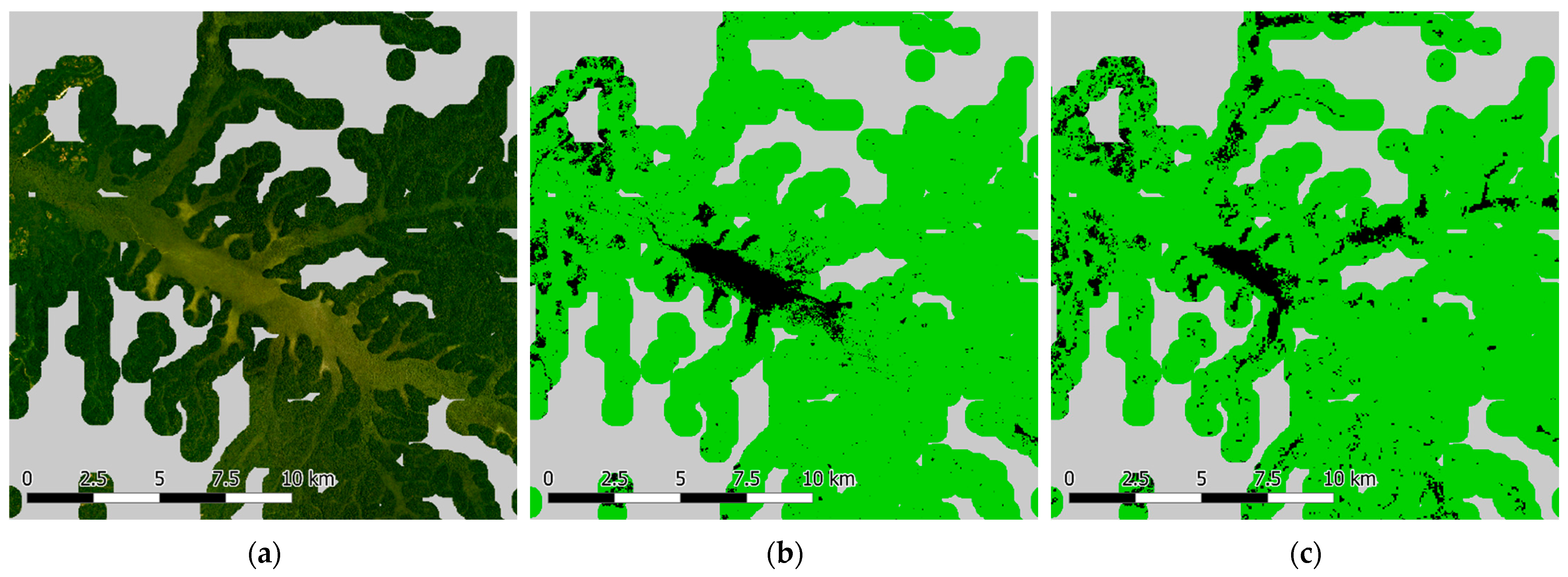
A major shortcoming of the state-of-the-art FNF masks is their poor performance in tropical wetland regions, where short vegetations (e.g., marshlands and shrubs) are often included in the forest class. Figure 1 shows two commonly used FNF products in tropical wetland areas. In the optical high-resolution PlanetScope reference image (Figure 1a), unforested wetland areas can be distinguished by their lighter colors, while forested wetlands are darker and rougher in texture. Both optical- and radar-based products overallocated the forest class to the unforested wetland regions (Figure 1b,c). The causes of the misclassification of these two products, however, are partly different in nature. As for the Landsat-based Global Forest Change product (Figure 1b), this is likely caused by the similar spectral signatures of forest and non-forest vegetation. For the radar-based DLR (German Aerospace Centre) FNF product, distinguishing forest and non-forest classes might be hindered by similar backscatter values of the short wavelength X-band radar and by frequent inundation [16]. Tropical wetlands have strong moisture dynamics, compared to moist tropical forests [17], greatly affecting the radar response [8,17]. Additionally, input data used for both FNF masks are insensitive to forest height, making it hard to distinguish different vegetated land cover classes. Over-estimating forest extent in a FNF mask poses a major issue for deforestation monitoring, often resulting in false positive detection of deforestation (high commission error) in wetland regions [7].
One way to discern forests from vegetated wetlands is to use a forest height product. Potapov et al. [19] recently combined data from the spaceborne Light Detection And Ranging (LiDAR) instrument Global Ecosystems Dynamics Investigation (GEDI) with Landsat time-series to generate a global forest height product at 30 m spatial resolution. Although relatively accurate FNF masks can be derived from this product alone [19], its local performance is substantially hindered by Landsat artifacts (e.g., Landsat 7 SLC-off stripes) [20] and cloud gaps in tropical regions. Other global, wall-to-wall forest height products exist [21,22,23], although these have a much coarser spatial resolution (500 m–1 km) and use input LiDAR data from before 2010. Combining a forest height product with radar data could improve the forest mapping accuracy and remove Landsat artifacts and cloud gaps from the resulting map [24]. As described by Joshi et al. [24], most of the shortcomings of optical data—from which the GEDI forest height product is partly derived [19]—and radar data are complementary and, therefore, show great combination potential. Sentinel-1 C-band radar data exhibit great potential with high spatial and temporal resolution and free access at a global scale [25]. No previous work, to the knowledge of the authors, has attempted to combine the GEDI-based Forest Height product with Sentinel-1 radar data for the purpose of forest mapping in wetlands.
Through the combination of GEDI-based forest heights and Sentinel-1 radar data in wetland regions of Gabon, this study aimed to improve the accuracy of FNF masks in tropical wetlands. We specifically aimed to assess the extent to which the combination improves the separation of forested and unforested wetland regions and reduces the presence of Landsat artifacts and cloud gaps in GEDI-based FNF masks.
2. Materials and Methods
2.1. Study Area
The wetland regions of Gabon, Central Africa, are taken as the study area (Figure 2). Gabon has a bimodal rainfall regime, with a long dry season in June–September and a short dry season in January–February [26]. Altitudes are below 50 m in much of the Ogooué River Delta in the West and reach as high as 1000 m in the mountain ranges further from the coast [27,28]. The predominant types of vegetation are primary tropical forest and (dry) savanna [26,29]. An estimation based on the global wetland map developed by the Center for International Forestry Research (CIFOR) revealed that Gabon holds 21,046 km2 of wetlands, translating to 8% of its surface area [30].
The Ogooué River Delta is the largest wetland region of Gabon (Figure 2) [31] and is under increasing anthropogenic threat due to, for example, agricultural expansion, oil and gas exploration and infrastructural projects [29]. Gabon’s wetland areas support local communities by providing clean drinking water and a habitat for many fish, birds, mammals and other species [29].
2.2. Data
An overview of the satellite data and products used for this study is given in Table 1. The study period was 1 January 2019 until 31 December 2019. The source and processing steps for each product are provided below. All products were resampled to a 30 m spatial resolution. We are aware of some of the resampling uncertainties, but these are not expected to greatly impact the results.
2.2.1. GEDI Forest Height Data
The 2019 GEDI-based Global Forest Canopy Height product (“GEDI Forest Height”) is a ready-to-use product that provides global forest height information at 30 m resolution [19] and was created by integrating LiDAR forest structure data from the spaceborne GEDI sensor with Landsat analysis-ready time-series data. Both the GEDI and Landsat data used for the forest height product are affected by Landsat artefacts and cloud gaps. In areas with persistent cloud cover, this leaves less imagery for the correction of Landsat 7 SLC-off stripes [20], introducing artifacts in the GEDI Forest Height product [19].
2.2.2. Sentinel-1 Radar Satellite Data
We used Sentinel-1 C-band Ground Range Detected (GRD) data acquired in both VV and VH polarizations. The Sentinel-1 data has a pixel spacing of 10 m and a revisit frequency of 5–12 days, depending on the exact geographic location [33]. In the study period (2019), Gabon was only covered by the Sentinel-1 satellites in descending orbit [34]. The GRD product was accessed through Google Earth Engine (GEE) [35]. Additional preprocessing was applied following the workflow suggested by Mulissa et al. [36] to remove border noise and terrain distortions, and to apply Lee speckle filtering [37].
We calculated backscatter temporal metrics (i.e., the mean, median, minimum, maximum, 5th percentile and 95th percentile) and texture features (the difference entropy of the mean backscatter value) individually for VV and VH. For the derivation of texture metrics, Lee filtering was not applied because it smooths important textural information. All metrics were resampled to the 30 m GEDI Forest Height product, using nearest neighbor resampling.
2.2.3. VHR Optical Data
Very High Resolution (VHR) optical data from PlanetScope were used as references for the creation of training and validation sets. Planet data have a resolution of 3.7 m [18], allowing for a more precise characterization of forest and non-forest in wetland areas compared to open-access alternatives such as Sentinel-2.
2.2.4. CIFOR Wetlands Data
The Global Wetlands (v3) dataset by CIFOR was used to specify wetlands in the study area. We applied a 500 m buffer to account for inaccuracies in the dataset and include the full wetland range. The data characterize 10 different wetland classes, including open water, mangrove, swamps, fens, riverine and lacustrine, floodplains and marshes, at a resolution of 231 m [31].
2.2.5. Global FNF Masks
Four global FNF masks were used for comparison against the mask developed in this study (Table 1). These masks vary in their spatial resolution and temporal coverage and employ slightly different forest definitions. The DLR FNF is based on data from the interferometric synthetic aperture radar (InSAR) system TanDEM-X, and has a 50 m resolution [14]. The JAXA FNF, with a resolution of 25 m, is derived from ALOS PALSAR [15]. Both of these products are resampled to a 30 m resolution. The Primary Tropical Forest mask is based on Landsat data, and limits the forest definition to “mature natural humid tropical forest cover”, thereby excluding regrown secondary forests [13]. Lastly, the Global Forest Change product—derived from the percent forest cover product with a cover threshold (80% in this study)—allocates all vegetation taller than 5 m and above a user-set forest cover threshold to the forest class [1].
The four FNF masks vary in their temporal coverage. We used the Global Forest Change product [1] to update all masks to the year 2019 by removing all deforested areas in the 2001–2019 period.
2.3. Methods
The general methodological approach involved first (Section 2.3.1) creating training and validation sets using Very High Resolution (VHR) optical PlanetScope data, then (Section 2.3.2) training and tuning a Random Forest (RF) model, and finally (Section 2.3.3), generating a FNF mask for wetland areas in Gabon that we compared against global FNF mask products—both quantitatively using a validation set and qualitatively by visual comparison. All analyses were conducted using the Google Earth Engine (https://earthengine.google.com/, accessed on 8 October 2021) and Python (v3.7).
2.3.1. Labeling the Training and Validation Sets
Due to the remoteness and poor navigability of the study area, typical for tropical regions, in situ data collection is costly and challenging [29]. Therefore, we resorted to PlanetScope mosaics and Sentinel-1 radar data to create labelled training and validation sets. The training set was used to train the RF model and assess the training performance. RF models are commonly used in pixel classification methods, mainly because of their efficiency, simplicity and high performance [38,39,40,41]. The validation set was used for independent validation of the resulting mask.
We adopted a functional forest definition, based on spectral and textural characteristics, instead of physical characteristics (e.g., numeric height). We defined forests as closed, high (based on shadows and texture) and undisturbed canopies, as seen in PlanetScope imagery. To clarify and standardize the labeling procedure, interpretation keys were defined for both classes (Table 2).
A total of 500 training locations distributed throughout the study area (CIFOR wetlands with 500 m buffer) were generated manually (Figure 2b), with an equal allocation to the forest and non-forest class. Manual selection was chosen over a regular grid, because it allows for choosing clean, unambiguous training locations. At each training location, we placed a 3 × 3 training point grid with 100 m point spacing. This resulted in a training set of 4500 training points with equal class allocation.
The validation set consisted of 1100 points, randomly distributed over the study area. The proportions of the validation set assigned to the forest and non-forest classes are 68% (748 points) and 32% (352 points), respectively, corresponding to the class proportions in the study area estimated using a preliminary classification model.
In situations where no cloud-free reference image was available, or the true class of the point was too ambiguous, we replaced that point with another randomly sampled point. In total, 62 points were replaced. Edges were labeled as non-forest, to account for the potential edge-shift between optical and radar imagery due to the side-looking of radar sensors. PlanetScope mosaic data also suffer from shifts between different time steps. Any point that fell outside of a forest area in one or more quarterly mosaics was labeled as non-forest.
2.3.2. Model Training and Tuning
Two different RF models were trained for this study: (i) using input features from Sentinel-1 data only (S1), and (ii) combining all features (GEDI-FH/S1). We also made a model with only GEDI Forest Height data (GEDI-FH), but since this ‘model’ only consisted of one feature, it was merely a matter of finding the right height threshold. The GEDI Forest Height product is affected by striped artifacts inherited from Landsat mosaics, leading to stripes of ‘nodata’ values in the models that use this data. To deal with the striping artifacts, the S1 model served as a substitute for the GEDI-FH/S1 model for pixels where the GEDI Forest Height was equal to zero.
The implementation of the RF model in GEE evaluates the Variable Importance (VI) for each feature by computing the sum over the decrease in Gini Impurity Index [42]. We used this score to enable a more thorough analysis of the contribution of each of the model’s features. Additionally, a Separability score was assigned to each feature, which defines how well the two classes can be distinguished based on their value distributions [43].
Four hyperparameters are available in the RF implementation in GEE: numberOfTrees, describing the number of decision trees in the model; variablesPerSplit, regulating the size of the (random) subset of input variables (i.e., features) that is available at each tree node; minLeafPopulation, determining the minimal number of points that should be present at each tree node; and maxNodes, defining the maximum number of nodes in each tree. For GEDI-FH/S1 and S1, we set numberOfTrees to 30, variablesPerSplit to the square root of the number of input variables (default), minLeafPopulation to 1 (default), and maxNodes to 30.
The Random Forest model returns a probability map, from which a binary FNF mask can be derived, given a certain probability threshold (PT). This Probability Threshold serves as a cut-off. All pixels with a forest probability below the threshold will be classified as non-forest, and vice versa. Altering the PT changes the mask’s accuracies, exposing a trade-off between over- or underestimating a certain class. In other words, the threshold can make the model more or less generous in allocating the forest class to the input data. Similarly, the forest height threshold in the GEDI-FH model can be altered to control the area to be allocated as forest from the GEDI Forest Height product. We assessed the effect of altering the PT from 10% to 90% in the S1 and GEDI-FH/S1 models, and the height thresholds from 5 m to 25 m in GEDI-FH model, on the accuracy of the final FNF masks.
2.3.3. Model Selection and Comparison with Existing FNF Masks
The training and validation User’s Accuracy (UA) and Producer’s Accuracy (PA) of the non-forest class were used to quantitatively analyze the FNF masks derived from S1, GEDI-FH/S1 and GEDI-FH with different thresholds, as well as the four masks from the literature (Table 1). The training and validation UA and PA were calculated using the training and independent validation set, respectively. We focused our analysis on the Producer’s Accuracy (omission error) of the non-forest class for two reasons. First, current FNF masks generally over-estimate the forest class in wetland regions (Figure 1). Second, in applying the FNF mask as a baseline for deforestation monitoring, commission errors carry a larger weight over omission errors, meaning that more conservative masks (i.e., those that were less likely to allocate the forest class) were preferred in this study.
Additionally, a visual comparison was carried out to assess the performance of GEDI-FH/S1 in three wetland areas located within the study area. We first explored the model’s performance at various PT (i.e., 20%, 40%, 60%, 80% and 90%). Then, a selection of these masks was compared against existing FNF masks. Specific attention was given to (i) the ability of each mask to discern non-forest areas, and (ii) the presence of Landsat artifacts in the FNF mask.
3. Results
3.1. Model Training and Feature Selection
The performance overview of the three models (Table 3) reveals very similar accuracies of both the GEDI-FH and the S1 models. The combination of all input features (GEDI-FH/S1) yields the best results, with a UA and PA of the non-forest class of 97.57% and 95.00%, respectively. Improvements are especially large in the detection of the non-forest class, as seen from the large increase in the non-forest PA.
The Separability and VI scores (Figure 3) show that the Forest Height and the two Sentinel-1 texture features achieve the highest scores on both metrics. The temporal backscatter statistics (i.e., mean, median, p0, p5, p95 and p100) generally perform poorly on the VI metric. For some features, such as the VH-median, VV-0th percentile and the VV-95th percentile, there is a large difference between the feature potential (Separability) and the actual importance of that feature in the trained model (VI).
3.2. Model Selection under Different Probability Thresholds (PTs)
Figure 4 shows the validation UA and PA for the non-forest class of the GEDI-FH/S1 model with varying PTs (a), and for the GEDI-FH model with varying height thresholds (b). Both models show a similar response to an increasing PT, with the UA and PA for the non-forest class balancing out at slightly over 70% accuracy.
Figure 5 depicts the FNF masks generated from the GEDI-FH/S1 model using increasing PTs for three detail maps of wetland areas located within the study area. PlanetScope imagery is provided for visual comparison. The maps reveal that the FNF mask is better able to discern non-forest patterns at higher PT values. In Area 1 and 2, most non-forest patches seem to be recognized by the mask with a PT of 80%. In Area 3, the model can discern small non-forest patches and roads at high PT values.
Considering both the quantitative and qualitative (visual) results, we decided to continue with 80% as the optimal PT for the GEDI-FH/S1 model, since it balances the UA and PA, without becoming too conservative in its allocation of the forest class (as can be seen at the 90% PT in Figure 5). We decided to use the 22.5 m height threshold for GEDI-FH, since it corresponds best with the 80% PT for GEDI-FH/S1, as seen from Figure 4.
3.3. Comparison with Existing FNF Masks
The validation UA and PA for the non-forest class of the four existing FNF masks, the best-performing variant of the GEDI-FH/S1 and GEDI-FH FNF masks, are presented in Table 4. The existing global FNF products perform poorly in terms of their ability to detect unforested areas in wetlands in the validation set, indicated by their relatively low PA (less than 54%). There are some notable differences between the existing masks. For example, the JAXA FNF seems to over-allocate the forest class, yielding a high UA (95%) but a low PA (32%). The other existing masks show the same characteristic, but to a lesser extent. The GEDI-FH/S1 model, with a PT of 80%, yields the highest PA (67.61%), indicating a stronger capacity in correctly detecting unforested areas in the wetlands. GEDI-FH, with a height threshold of 22.5 m, yields a similar performance, but is slightly more generous in allocating the forest class.
Figure 6 presents detail maps of optical PlanetScope imagery, JAXA FNF, DLR FNF, the Global Forest Change, the FNF mask from the best GEDI-FH model (with a 22.5 m threshold) and the FNF mask from the best GEDI-FH/S1 model (with a PT of 80%), for the same three example wetland areas as in Figure 5. The DLR FNF and Global Forest Change masks are generally the most generous masks, allocating the forest class to many unforested areas (as seen in the PlanetScope imagery). The Global Forest Change and the FNF mask from the GEDI-FH/S1 model can both discern the roads in Area 3 to some extent.
Comparing the best GEDI-FH mask with the best GEDI-FH/S1 mask, we observe that the latter is more conservative in allocating the forest class. The GEDI-FH/S1 mask preserves the sharp forest edges (in Area 1 and 2) and produces a smoother (less grainy) result. In addition, the GEDI-FH mask suffers from Landsat artifacts (Area 3), recognized by the diagonal black stripes (Figure 6q), while the GEDI-FH/S1 mask does not.
4. Discussion
4.1. Model Training
The training results reveal that a RF model combining GEDI Forest Height data with Sentinel-1 temporal and texture metrics (GEDI-FH/S1) outperforms models that only use either of these input feature sets (GEDI-FH and S1) (Table 3). A similar observation can be made from the Separability and VI scores of all individual features. The Forest Height feature and the texture features (for both VV and VH polarizations) all have a high VI in the RF model and show a high Separability of the class distributions. This indicates a high classification potential for these three features and explains the high training and validation accuracies of the GEDI-FH/S1 model.
These results suggest that the combination of features proposed in this study aids the training of a FNF model in wetland areas. We hypothesize that this synergy arises because the two data sources compensate for each other’s shortcomings: the forest height data help to distinguish short vegetation and tall vegetation, in which radar data fall short because of moisture dynamics. On the other hand, Landsat artifacts in the forest height data are overcome with the radar data.
4.2. Selecting a FNF Mask for Deforestation Monitoring
This study demonstrated how GEDI Forest Height data, aided by Sentinel-1 radar data, can be used to achieve considerable improved FNF masks in tropical wetland regions. The combination enhances the ability of a RF-based model (GEDI-FH/S1) to detect non-forest areas in wetlands, by excluding areas with low vegetation height from the forest class.
Analyzing the resultant FNF masks of the GEDI-FH/S1 model with different PTs shows a clear trade-off between the UA and PA (Figure 4). To minimize false detection in radar-based deforestation monitoring requires a conservative FNF mask that minimizes false deforestation detections, which are considered worse than omitted detections [7]. We selected a high PT (80%) to obtain a conservative FNF mask. The suggested PT, however, may not be appropriate for other applications, such as forest extent mapping, but can be tuned to certain needs.
The CIFOR global wetlands dataset, used to define the study area, has a limited spatial accuracy (locally) and, therefore, might fall short in delineating the Gabonese wetlands. The major advantage of the CIFOR dataset over other (local and regional) wetland datasets is its global coverage, which can support the expansion of the approach to continental or pan-tropical scales. We used a 500 m buffer around the CIFOR data to partly overcome the inaccuracies. Inevitably, non-wetland land cover types were present in the training data. Using a more accurate local or regional wetland map would result in a ‘cleaner’ training set, which would be likely to ease the training process and improve the validation results in a local-to-regional context.
4.3. Comparison with Existing FNF Masks
The FNF mask developed for wetlands in Gabon in this study yields high validation accuracies compared to existing global FNF mask products. Particularly, the GEDI-FH/S1 model’s ability to uncover non-forest areas, with a validation PA for non-forest reaching 70%, is much higher than that of existing FNF masks, which is generally less than 54%. Although we do recognize that a PA of 70% for non-forest areas is not ideal, it is a considerable improvement of the state-of-the-art performance in wetland regions and emphasizes the complexity of accurately mapping wetlands. The differences among the existing FNF masks are expected to be caused mainly by differing forest definitions, data sources and characteristics (e.g., optical vs. radar, and different radar wavelengths), pixel spacings, and temporal coverages.
We compared the GEDI-FH/S1 model with a simple model derived from only GEDI Forest Height data (GEDI-FH). Both models yield very similar quantitative results. However, a clear difference between the products can be seen in the qualitative (visual) comparison (Figure 6). The GEDI-FH/S1 model is much better able to discern complex non-forest patterns in Gabon’s wetlands, which is likely caused by the inclusion of Sentinel-1 texture data.
Additionally, the inclusion of Sentinel-1 data has the potential to alleviate the impact of Landsat artifacts in the input data, by performing the substitution described in Section 2.3.3. The substitution method has effectively removed the artifacts from our mask, without compromising the general classification performance.
5. Conclusions
In this study, a methodology was presented to improve the accuracy of FNF masks in tropical wetlands by combining GEDI Forest Height data and Sentinel-1 radar data in a Random Forest model. The training results reveal that the combination of GEDI Forest Height data and Sentinel-1 data enhances the model’s ability to discern unforested wetlands. Quantitatively, our model yields the highest non-forest PA of all (existing) masks we compared it with, but overall scores are similar to a Forest Height-only model. Qualitatively, however, our mask can overcome Landsat artifacts present in the Forest Height-only mask and is much better able to discern complex non-forest patterns. An additional advantage of the methodology presented here is that it can be tailored to different applications by varying the PT.
This study showed that global land cover (here: forest) products, when improved to fit a specific context (here: wetlands), can be used for various (local) applications. We stress that, in any application of the suggested FNF mask, it is important to consider the UA/PA trade-off and the effect it has on the classification. In addition, wetland characteristics might be very different in other regions, and this might necessitate changes to the methodology, such as the use of a different sampling strategy and/or forest definition. The targeted improvements for wetland forest mapping presented in this paper can help raise the accuracy of tropical deforestation monitoring and alerting.
Author Contributions
Conceptualization, K.V., J.R. and Y.G.; methodology, K.V., J.R. and Y.G.; software, K.V.; validation, K.V., J.R. and Y.G.; formal analysis, K.V.; investigation, K.V.; writing—original draft preparation, K.V.; writing—review and editing, J.R., Y.G. and M.H.; visualization, K.V.; supervision, J.R. and Y.G.; project administration, J.R.; funding acquisition, J.R. All authors have read and agreed to the published version of the manuscript.
Funding
This research received funding through Norway’s Climate and Forest Initiative (NICFI) and the US Government’s SilvaCarbon program.
Data Availability Statement
The data that support the findings of this study are available upon reasonable request from the authors.
Acknowledgments
Planet data were provided through the Planet ambassador program. This study used modified Copernicus Sentinel data (2019). We thank Nandika Tsendbazar from Wageningen University for her advice on accuracy assessment.
Conflicts of Interest
The authors declare no conflict of interest. The funders had no role in the design of the study; in the collection, analyses, or interpretation of data; in the writing of the manuscript, or in the decision to publish the results.
Appendix A
Figure A1.
Sensitivity of the Global Forest Change mask performance for a varying canopy cover percentage.
Figure A1.
Sensitivity of the Global Forest Change mask performance for a varying canopy cover percentage.

References
- Hansen, M.C.; Potapov, P.V.; Moore, R.; Hancher, M.; Turubanova, S.A.; Tyukavina, A.; Thau, D.; Stehman, S.V.; Goetz, S.J.; Loveland, T.R.; et al. High-resolution global maps of 21st-century forest cover change. Science 2013, 342, 850–853. [Google Scholar] [CrossRef] [PubMed] [Green Version]
- Roopsind, A.; Sohngen, B.; Brandt, J. Evidence that a national REDD+ program reduces tree cover loss and carbon emissions in a high forest cover, low deforestation country. Proc. Natl. Acad. Sci. USA 2019, 116, 24492–24499. [Google Scholar] [CrossRef]
- Pickering, J.; Tyukavina, A.; Khan, A.; Potapov, P.; Adusei, B.; Hansen, M.C.; Lima, A. Using Multi-Resolution Satellite Data to Quantify Land Dynamics: Applications of PlanetScope Imagery for Cropland and Tree-Cover Loss Area Estimation. Remote Sens. 2021, 13, 2191. [Google Scholar] [CrossRef]
- Beuchle, R.; Grecchi, R.C.; Shimabukuro, Y.E.; Seliger, R.; Eva, H.D.; Sano, E.; Achard, F. Land cover changes in the Brazilian Cerrado and Caatinga biomes from 1990 to 2010 based on a systematic remote sensing sampling approach. Appl. Geogr. 2015, 58, 116–127. [Google Scholar] [CrossRef]
- Harris, N.L.; Gibbs, D.A.; Baccini, A.; Birdsey, R.A.; de Bruin, S.; Farina, M.; Fatoyinbo, L.; Hansen, M.C.; Herold, M.; Houghton, R.A.; et al. Global maps of twenty-first century forest carbon fluxes. Nat. Clim. Chang. 2021, 11, 234–240. [Google Scholar] [CrossRef]
- Hansen, M.C.; Krylov, A.; Tyukavina, A.; Potapov, P.V.; Turubanova, S.; Zutta, B.; Ifo, S.; Margono, B.; Stolle, F.; Moore, R. Humid tropical forest disturbance alerts using Landsat data. Environ. Res. Lett. 2016, 11, 034008. [Google Scholar] [CrossRef]
- Reiche, J.; Mullissa, A.; Slagter, B.; Gou, Y.; Tsendbazar, N.-E.; Odongo-Braun, C.; Vollrath, A.; Weisse, M.J.; Stolle, F.; Pickens, A.; et al. Forest disturbance alerts for the Congo Basin using Sentinel-1. Environ. Res. Lett. 2021, 16, 024005. [Google Scholar] [CrossRef]
- Reiche, J.; Hamunyela, E.; Verbesselt, J.; Hoekman, D.; Herold, M. Improving near-real time deforestation monitoring in tropical dry forests by combining dense Sentinel-1 time series with Landsat and ALOS-2 PALSAR-2. Remote Sens. Environ. 2018, 204, 147–161. [Google Scholar] [CrossRef]
- Finer, M.; Novoa, S.; Weisse, M.J.; Petersen, R.; Mascaro, J.; Souto, T.; Stearns, F.; Martinez, R.G. Combating deforestation: From satellite to intervention. Science 2018, 360, 1303–1305. [Google Scholar] [CrossRef]
- Kissinger, G.; Herold, M.; De Sy, V. Drivers of Deforestation and Forest Degradation: A Synthesis Report for REDD+ Policymakers; Lexeme Consulting: Vancouver, BC, Canada, 2012. [Google Scholar]
- Hansen, M.C.; Wang, L.; Song, X.-P.; Tyukavina, A.; Turubanova, S.; Potapov, P.V.; Stehman, S.V. The fate of tropical forest fragments. Sci. Adv. 2020, 6, eaax8574. [Google Scholar] [CrossRef] [Green Version]
- Nunes, L.J.R.; Meireles, C.I.R.; Pinto Gomes, C.J.; Almeida Ribeiro, N.M.C. Forest Contribution to Climate Change Mitigation: Management Oriented to Carbon Capture and Storage. Climate 2020, 8, 21. [Google Scholar] [CrossRef] [Green Version]
- Turubanova, S.; Potapov, P.V.; Tyukavina, A.; Hansen, M.C. Ongoing primary forest loss in Brazil, Democratic Republic of the Congo, and Indonesia. Environ. Res. Lett. 2018, 13, 074028. [Google Scholar] [CrossRef] [Green Version]
- Martone, M.; Rizzoli, P.; Wecklich, C.; González, C.; Bueso-Bello, J.L.; Valdo, P.; Schulze, D.; Zink, M.; Krieger, G.; Moreira, A. The global forest/non-forest map from TanDEM-X interferometric SAR data. Remote Sens. Environ. 2018, 205, 352–373. [Google Scholar] [CrossRef]
- Shimada, M.; Itoh, T.; Motooka, T.; Watanabe, M.; Shiraishi, T.; Thapa, R.; Lucas, R. New global forest/non-forest maps from ALOS PALSAR data (2007–2010). Remote Sens. Environ. 2014, 155, 13–31. [Google Scholar] [CrossRef]
- Dargie, G.C.; Lewis, S.L.; Lawson, I.T.; Mitchard, E.T.A.; Page, S.E.; Bocko, Y.E.; Ifo, S.A. Age, extent and carbon storage of the central Congo Basin peatland complex. Nature 2017, 542, 86–90. [Google Scholar] [CrossRef]
- Jensen, K.; McDonald, K.; Podest, E.; Rodriguez-Alvarez, N.; Horna, V.; Steiner, N. Assessing L-Band GNSS-Reflectometry and Imaging Radar for Detecting Sub-Canopy Inundation Dynamics in a Tropical Wetlands Complex. Remote Sens. 2018, 10, 1431. [Google Scholar] [CrossRef] [Green Version]
- Potapov, P.; Li, X.; Hernandez-Serna, A.; Tyukavina, A.; Hansen, M.C.; Kommareddy, A.; Pickens, A.; Turubanova, S.; Tang, H.; Silva, C.E.; et al. Mapping global forest canopy height through integration of GEDI and Landsat data. Remote Sens. Environ. 2021, 253, 112165. [Google Scholar] [CrossRef]
- Wulder, M.A.; Ortlepp, S.M.; White, J.C.; Maxwell, S. Evaluation of Landsat-7 SLC-off image products for forest change detection. Can. J. Remote Sens. 2008, 34, 93–99. [Google Scholar] [CrossRef]
- Lefsky, M.A. A global forest canopy height map from the Moderate Resolution Imaging Spectroradiometer and the Geoscience Laser Altimeter System. Geophys. Res. Lett. 2010, 37. [Google Scholar] [CrossRef] [Green Version]
- Simard, M.; Pinto, N.; Fisher, J.B.; Baccini, A. Mapping forest canopy height globally with spaceborne lidar. J. Geophys. Res. 2011, 116, G04021. [Google Scholar] [CrossRef] [Green Version]
- Wang, Y.; Li, G.; Ding, J.; Guo, Z.; Tang, S.; Wang, C.; Huang, Q.; Liu, R.; Chen, J.M. A combined GLAS and MODIS estimation of the global distribution of mean forest canopy height. Remote Sens. Environ. 2016, 174, 24–43. [Google Scholar] [CrossRef]
- Joshi, N.; Baumann, M.; Ehammer, A.; Fensholt, R.; Grogan, K.; Hostert, P.; Jepsen, M.; Kuemmerle, T.; Meyfroidt, P.; Mitchard, E.; et al. A Review of the Application of Optical and Radar Remote Sensing Data Fusion to Land Use Mapping and Monitoring. Remote Sens. 2016, 8, 70. [Google Scholar] [CrossRef] [Green Version]
- Ruiz-Ramos, J.; Marino, A.; Boardman, C.; Suarez, J. Continuous Forest Monitoring Using Cumulative Sums of Sentinel-1 Timeseries. Remote Sens. 2020, 12, 3061. [Google Scholar] [CrossRef]
- Bogning, S.; Frappart, F.; Paris, A.; Blarel, F.; Niño, F.; Saux Picart, S.; Lanet, P.; Seyler, F.; Mahé, G.; Onguene, R.; et al. Hydro-climatology study of the Ogooué River basin using hydrological modeling and satellite altimetry. Adv. Sp. Res. 2020, 68, 672–690. [Google Scholar] [CrossRef]
- ESA. Copernicus Copernicus DEM: 30 Meter Dataset Now Publicly Available. 2021. Available online: https://spacedata.copernicus.eu/blogs/-/blogs/copernicus-dem-30-meter-dataset-now-publicly-available (accessed on 8 October 2021).
- AIRBUS. Copernicus DEM: Copernicus Digital Elevation Model Product Handbook. 2020. Available online: https://spacedata.copernicus.eu/documents/20126/0/GEO1988-CopernicusDEM-SPE-002_ProductHandbook_I1.00.pdf/082dd479-f908-bf42-51bf-4c0053129f7c?t=1586526993604 (accessed on 8 October 2021).
- Aldous, A.; Schill, S.; Raber, G.; Paiz, M.C.; Mambela, E.; Stévart, T. Mapping complex coastal wetland mosaics in Gabon for informed ecosystem management: Use of object-based classification. Remote Sens. Ecol. Conserv. 2020, 7, 64–79. [Google Scholar] [CrossRef]
- Gumbricht, T.; Roman-Cuesta, R.M.; Verchot, L.; Herold, M.; Wittmann, F.; Householder, E.; Herold, N.; Murdiyarso, D. An expert system model for mapping tropical wetlands and peatlands reveals South America as the largest contributor. Glob. Chang. Biol. 2017, 23, 3581–3599. [Google Scholar] [CrossRef] [Green Version]
- Murdiyarso, D.; Román-Cuesta, R.M.; Verchot, L.; Herold, M.; Gumbricht, T.; Herold, N.; Martius, C. New Map Reveals More Peat in the Tropics; Center for International Forestry Research (CIFOR). 2017. Available online: https://www.cifor.org/publications/pdf_files/infobrief/6452-infobrief.pdf (accessed on 8 October 2021).
- Fichet, L.; Sannier, C.; Makaga, E.M.K.; Seyler, F. Assessing the Accuracy of Forest Cover Map for 1990, 2000 and 2010 at National Scale in Gabon. IEEE J. Sel. Top. Appl. Earth Obs. Remote Sens. 2014, 7, 1346–1356. [Google Scholar] [CrossRef]
- Torres, R.; Snoeij, P.; Geudtner, D.; Bibby, D.; Davidson, M.; Attema, E.; Potin, P.; Rommen, B.; Floury, N.; Brown, M.; et al. GMES Sentinel-1 mission. Remote Sens. Environ. 2012, 120, 9–24. [Google Scholar] [CrossRef]
- Planet. Planet Imagery Product Specifications. 2020. Available online: https://assets.planet.com/docs/Planet_Combined_Imagery_Product_Specs_letter_screen.pdf (accessed on 8 October 2021).
- ESA. Sentinel-1 Observation Scenario. Available online: https://sentinels.copernicus.eu/web/sentinel/missions/sentinel-1/observation-scenario (accessed on 31 May 2021).
- Google Earth Engine. Sentinel-1 Algorithms. Available online: https://developers.google.com/earth-engine/guides/sentinel1 (accessed on 15 February 2021).
- Mullissa, A.; Vollrath, A.; Odongo-Braun, C.; Slagter, B.; Balling, J.; Gou, Y.; Gorelick, N.; Reiche, J. Sentinel-1 SAR Backscatter Analysis Ready Data Preparation in Google Earth Engine. Remote Sens. 2021, 13, 1954. [Google Scholar] [CrossRef]
- Lee, J.-S.; Wen, J.-H.; Ainsworth, T.L.; Chen, K.-S.; Chen, A.J. Improved Sigma Filter for Speckle Filtering of SAR Imagery. IEEE Trans. Geosci. Remote Sens. 2009, 47, 202–213. [Google Scholar] [CrossRef]
- Sano, E.E.; Rizzoli, P.; Koyama, C.N.; Watanabe, M.; Adami, M.; Shimabukuro, Y.E.; Bayma, G.; Freitas, D.M. Comparative analysis of the global forest/non-forest maps derived from sar and optical sensors. Case studies from brazilian amazon and cerrado biomes. Remote Sens. 2021, 13, 367. [Google Scholar] [CrossRef]
- Hirschmugl, M.; Sobe, C.; Deutscher, J.; Schardt, M. Combined Use of Optical and Synthetic Aperture Radar Data for REDD+ Applications in Malawi. Land 2018, 7, 116. [Google Scholar] [CrossRef] [Green Version]
- Crowson, M.; Warren-Thomas, E.; Hill, J.K.; Hariyadi, B.; Agus, F.; Saad, A.; Hamer, K.C.; Hodgson, J.A.; Kartika, W.D.; Lucey, J.; et al. A comparison of satellite remote sensing data fusion methods to map peat swamp forest loss in Sumatra, Indonesia. Remote Sens. Ecol. Conserv. 2019, 5, 247–258. [Google Scholar] [CrossRef] [Green Version]
- Jin, Y.; Liu, X.; Chen, Y.; Liang, X. Land-cover mapping using Random Forest classification and incorporating NDVI time-series and texture: A case study of central Shandong. Int. J. Remote Sens. 2018, 39, 8703–8723. [Google Scholar] [CrossRef]
- Afanador, N.L.; Smolinska, A.; Tran, T.N.; Blanchet, L. Unsupervised random forest: A tutorial with case studies. J. Chemom. 2016, 30, 232–241. [Google Scholar] [CrossRef]
- Hansen, J.N.; Mitchard, E.T.A.; King, S. Assessing Forest/Non-Forest Separability Using Sentinel-1 C-Band Synthetic Aperture Radar. Remote Sens. 2020, 12, 1899. [Google Scholar] [CrossRef]
Figure 1.
A comparison of: (a) a true-color, optical image from PlanetScope [18]; (b) the optical-based Global Forest Change product [1]; and (c) the radar-based FNF mask from German Aerospace Centre (DLR) [14]. The Global Forest Change loss product for 2000–2019 [1] was used in (b,c) to exclude areas that were deforested in that period. The area is in Eastern Gabon (14.0683 E, 0.9783 N). The area is masked to only show (buffered) wetland pixels; the others are grey. Pixels classified as forest are shown in green; non-forest areas are shown in black.

Figure 2.
Wetland distribution in Gabon (CIFOR wetlands) (a) and the spatial distribution of training clusters (500 clusters in total with 9 points for each cluster) and validation points (1100 points in total) (b).
Figure 2.
Wetland distribution in Gabon (CIFOR wetlands) (a) and the spatial distribution of training clusters (500 clusters in total with 9 points for each cluster) and validation points (1100 points in total) (b).

Figure 3.
Separability and VI scores for all input features in this study. The importance scores are taken from the GEDI-FH/S1 model configuration. The feature names for the Sentinel-1 data are composed of their polarization (VV/VH) and their statistic (mean, median or a percentile; e.g., ‘VV_p95′ for the 95th percentile of the VV polarization image). Texture features are suffixed with ‘tex’.

Figure 4.
UA and PA of the non-forest (NF) class for the GEDI-FH/S1 model for increasing PT values (a) and for the GEDI-FH model for increasing height threshold values (b).
Figure 4.
UA and PA of the non-forest (NF) class for the GEDI-FH/S1 model for increasing PT values (a) and for the GEDI-FH model for increasing height threshold values (b).

Figure 5.
Detail maps comparing GEDI-FH/S1 masks with different PTs in three wetland regions in Gabon (a–r). PlanetScope imagery is also given for reference. Only areas within the 500 m CIFOR wetland buffer are considered as the study region; other areas are masked out in grey. Forest is shown in green and non-forest in black.

Figure 6.
Detail maps comparing FNF masks in three different wetland regions in Gabon (a–r). PlanetScope imagery is also given for reference. Only areas within the 500 m CIFOR wetland buffer are considered as the study region; other areas are masked out in grey. Forest is shown in green and non-forest in black.


Table 1.
Overview of the satellite data and products used in this study. * The FNF masks were updated to the year 2019 by removing annual forest loss information available via the Global Forest Change product [1].
Table 1.
Overview of the satellite data and products used in this study. * The FNF masks were updated to the year 2019 by removing annual forest loss information available via the Global Forest Change product [1].
| Data Source | Pixel Spacing | Temporal Resolution | Temporal Coverage | Data Function | Reference | ||
|---|---|---|---|---|---|---|---|
| GEDI Forest Height data | Landsat, GEDI | 30 m | – | 2019 | Input feature | [19] | |
| Radar data | Sentinel-1 | 10 m | 5–12 days | 1 January 2019– 31 December 2019 | Input feature | [33] | |
| VHR Optical data | PlanetScope | 3.7 m | Quarterly | 1 January 2019– 31 December 2019 | Generating training and validation dataset | [18] | |
| CIFOR Wetlands data | Various RS data combined | 231 m | – | 2011 | Define wetland areas | [31] | |
| Existing FNF Masks | DLR FNF | TanDEM-X | 50 m | – | 2011–2015 * | Comparison | [14] |
| JAXA FNF | ALOS PALSAR | 25 m | – | 2015 * | Comparison | [15] | |
| Primary Tropical Forest | Landsat | 30 m | – | 2001 * | Comparison | [13] | |
| Global Forest Change | Landsat | 30 m | – | 2001 * | Comparison and to update all FNF to 2019 | [1] | |
Table 2.
Interpretation keys for labeling forest/non-forest training and validation points. F = Forest; NF = Non-Forest.
Table 2.
Interpretation keys for labeling forest/non-forest training and validation points. F = Forest; NF = Non-Forest.
| Class | Interpretation Key | Image Example |
|---|---|---|
| Forest | Color (true color RGB): dark green Texture: rough Cover type: medium to dense canopy cover |  |
| Non-forest | Color (true color RGB): light green Texture: smooth Cover type: sparse to no canopy cover; bushes/shrubs |
Table 3.
Training accuracies of non-forest class generated using the GEDI-FH, S1, and GEDI-FH/S1 models. All masks are generated from the RF probability output at a PT of 50%.
Table 3.
Training accuracies of non-forest class generated using the GEDI-FH, S1, and GEDI-FH/S1 models. All masks are generated from the RF probability output at a PT of 50%.
| Training Results (n = 4500) | Non-Forest | ||
|---|---|---|---|
| Model | Feature Set | UA (%) | PA (%) |
| GEDI-FH | GEDI Forest Height | 94.99 | 84.18 |
| S1 | Sentinel-1 (temporal metrics; texture) | 95.06 | 85.56 |
| GEDI-FH/S1 | GEDI Forest Height, Sentinel-1 (temporal metrics; texture) | 97.57 | 95.00 |
Table 4.
Validation UA and PA for existing FNF masks and resultant FNF masks from GEDI-FH and GEDI-FH/S1. * A more in-depth analysis of how the validation UA and PA is affected by an increasing cover threshold can be found in Figure A1.
Table 4.
Validation UA and PA for existing FNF masks and resultant FNF masks from GEDI-FH and GEDI-FH/S1. * A more in-depth analysis of how the validation UA and PA is affected by an increasing cover threshold can be found in Figure A1.
| Validation Results (n = 1100) | Non-Forest | |
|---|---|---|
| Feature Set | UA (%) | PA (%) |
| DLR FNF | 89.53 | 48.58 |
| JAXA FNF | 95.00 | 32.39 |
| Primary Tropical Forest | 86.60 | 47.73 |
| Global Forest Change (canopy cover: 80% *) | 88.37 | 53.98 |
| GEDI-FH/S1 (PT: 80%) | 77.78 | 67.61 |
| GEDI-FH (height: 22.5 m) | 78.41 | 67.05 |
Publisher’s Note: MDPI stays neutral with regard to jurisdictional claims in published maps and institutional affiliations. |
© 2021 by the authors. Licensee MDPI, Basel, Switzerland. This article is an open access article distributed under the terms and conditions of the Creative Commons Attribution (CC BY) license (https://creativecommons.org/licenses/by/4.0/).
Share and Cite
MDPI and ACS Style
Verhelst, K.; Gou, Y.; Herold, M.; Reiche, J. Improving Forest Baseline Maps in Tropical Wetlands Using GEDI-Based Forest Height Information and Sentinel-1. Forests 2021, 12, 1374. https://0-doi-org.brum.beds.ac.uk/10.3390/f12101374
AMA Style
Verhelst K, Gou Y, Herold M, Reiche J. Improving Forest Baseline Maps in Tropical Wetlands Using GEDI-Based Forest Height Information and Sentinel-1. Forests. 2021; 12(10):1374. https://0-doi-org.brum.beds.ac.uk/10.3390/f12101374
Chicago/Turabian StyleVerhelst, Kamiel, Yaqing Gou, Martin Herold, and Johannes Reiche. 2021. "Improving Forest Baseline Maps in Tropical Wetlands Using GEDI-Based Forest Height Information and Sentinel-1" Forests 12, no. 10: 1374. https://0-doi-org.brum.beds.ac.uk/10.3390/f12101374
Note that from the first issue of 2016, this journal uses article numbers instead of page numbers. See further details here.