
Best Practices for Quasistatic Berkovich Nanoindentation of Wood Cell Walls


1
Forest Biopolymers Science and Engineering, USDA Forest Service, Forest Products Laboratory, One Gifford Pinchot Drive, Madison, WI 53726, USA
2
Department of Materials Science and Engineering, University of Wisconsin—Madison, 1509 University Avenue, Madison, WI 53706, USA
*
Author to whom correspondence should be addressed.
Forests 2021, 12(12), 1696; https://0-doi-org.brum.beds.ac.uk/10.3390/f12121696
Submission received: 2 November 2021
/
Revised: 22 November 2021
/
Accepted: 27 November 2021
/
Published: 3 December 2021
(This article belongs to the Special Issue Nanoindentation in Wood)
Abstract
:For wood and forest products to reach their full potential as structural materials, experimental techniques are needed to measure mechanical properties across all length scales. Nanoindentation is uniquely suited to probe in situ mechanical properties of micrometer-scale features in forest products, such as individual wood cell wall layers and adhesive bondlines. However, wood science researchers most commonly employ traditional nanoindentation methods that were originally developed for testing hard, inorganic materials, such as metals and ceramics. These traditional methods assume that the tested specimen is rigidly supported, homogeneous, and semi-infinite. Large systematic errors may affect the results when these traditional methods are used to test complex polymeric materials, such as wood cell walls. Wood cell walls have a small, finite size, and nanoindentations can be affected by nearby edges. Wood cell walls are also not rigidly supported, and the cellular structure can flex under loading. Additionally, wood cell walls are softer and more prone to surface detection errors than harder inorganic materials. In this paper, nanoindentation methods for performing quasistatic Berkovich nanoindentations, the most commonly applied nanoindentation technique in forest products research, are presented specifically for making more accurate nanoindentation measurements in materials such as wood cell walls. The improved protocols employ multiload nanoindentations and an analysis algorithm to correct and detect errors associated with surface detection errors and structural compliances arising from edges and specimen-scale flexing. The algorithm also diagnoses other potential issues arising from dirty probes, nanoindenter performance or calibration issues, and displacement drift. The efficacy of the methods was demonstrated using nanoindentations in loblolly pine (Pinus taeda) S2 cell wall layers (S2) and compound corner middle lamellae (CCML). The nanoindentations spanned a large range of sizes. The results also provide new guidelines about the minimum size of nanoindentations needed to make reliable nanoindentation measurements in S2 and CCML.
1. Introduction
Over the past 25 years, nanoindentation has become a valuable tool in wood science and forest products research. Nanoindentation is a type of instrumented indentation experiment used most often to measure mechanical properties, such as elastic modulus and hardness [1,2]. Elastic modulus quantifies a material’s stiffness or resistance to elastic (recoverable) deformation under stress. Hardness quantifies a material’s resistance to plastic or permanent deformations. An advantage of nanoindentation over other mechanical testing techniques is its ability to probe micrometer-scale volumes of materials in situ with a minimal amount of sample preparation. This makes nanoindentation ideally suited for probing individual wood cell wall layers, such as the S2 cell wall layer (S2) and compound corner middle lamella (CCML) (Figure 1), and other micrometer-scale features in wood-based materials, such as wood-adhesive bondlines in laminated structures, wood-matrix interphase regions in wood-based composites, and coatings on engineered wood products. Often, nanoindentation is the only technique suitable for studying the mechanical properties and effects of treatments in these small volumes of material.
Since the pioneering work of Wimmer and co-workers, who first used nanoindentation to measure the mechanical properties of the S2 and CCML [6,7], nanoindentation has been extensively employed to measure micromechanical properties in wood and forest products. These efforts provide valuable information over a wide range of research areas, including fundamental cell wall properties [8,9,10,11,12,13,14,15,16,17], reaction wood [18,19,20,21], moisture-dependent properties [22,23,24,25,26,27], temperature-dependent properties [28,29], wood-adhesive bondlines [30,31,32,33,34,35,36,37,38], coatings [39,40,41,42], wood–plastic composites [43,44,45,46,47], chemical modification [48,49,50,51,52,53], thermal modification [54,55,56,57,58,59], biodegradation [60,61,62,63], chemical degradation [64,65,66,67,68], enzymatic degradation [69,70], pyrolysis [71,72,73], hot water extraction [74,75], kiln drying [76], archaeological wood [77,78,79,80], and petrified wood [81].
Most often, forest products researchers have made hardness and elastic modulus measurements by employing quasistatic Berkovich probe nanoindentations analyzed using the traditional Oliver–Pharr analysis method [2]. In quasistatic nanoindentation, only loads and depths are measured as a function of time during the experiments, and mechanical properties are determined from an analysis of the resulting load–depth trace. This contrasts with dynamic nanoindentation, in which a small sinusoidal signal is superimposed on the static load to facilitate the measurement of stiffnesses, and therefore mechanical properties, continuously during the experiment [2,82,83,84]. The Berkovich probe is a three-sided pyramid defined by a 65.27° angle between the pyramid longitudinal axis and a pyramid face [85]. The “Oliver–Pharr method” has become synonymous with the traditional nanoindentation analysis used to calculate hardness and elastic modulus, which is described in detail in Section 2.2, even though not all components of the analysis come directly from the original Oliver–Pharr paper published in 1992 [2]. The traditional nanoindentation analysis generally consists of performing fused silica calibration experiments to calculate the nanoindenter machine compliance and probe area function. Then, these calibrations are used in an analysis of the test material load–depth trace to calculate hardness and elastic modulus.
The traditional nanoindentation method includes both experimental protocols for performing nanoindentation and an analysis for the load–depth trace. These methods were originally developed to test hard, inorganic materials, such as metals and ceramics. Additionally, these methods assume the tested specimen is either a bulk, homogeneous material or a thin-film-substrate configuration in which the film–substrate interface is parallel to the tested surface. In contrast, wood cell walls are much softer than metals or ceramics and are more prone to surface detection errors. Nanoindentations placed in unembedded wood cell walls are also always near interfaces and edges, such as the free edge formed by the cell wall and empty lumen, and the entire wood cellular structure can flex under loading. Both edge effects and specimen-scale flexing violate the assumptions of the traditional nanoindentation analysis.
Nanoindentation probes also have a much higher propensity to pick up debris and become dirty during nanoindentation in wood than in experiments in traditional hard materials. Traditional material surfaces are relatively free of debris because they are either pristinely deposited thin films or have been thoroughly cleaned with solvents following polishing. Wood nanoindentation surfaces cannot be similarly cleaned, and any debris created during surface preparation will remain on the surface. Additionally, in traditional bulk materials, nanoindentations can often be performed in regular arrays without having to target specific features on the surface. In this case, the probe tip is lifted off the surface between nanoindentation sites, and contact with the surface is only made during the indentation measurement. In contrast, in wood, the probe tip is typically raster-scanned over the surface under a small load to create topographic scanning probe microscopy (SPM) images that are used to precisely place nanoindentations in the regions of interest. The probe tip has many more opportunities to pick up debris and become dirty during raster scanning than during traditional array experiments. During a series of nanoindentations, the tip may sporadically pick up debris during some indents and then release the debris during others. Detecting randomly dirty probes during nanoindentation in wood cell walls is very difficult using traditional methods.
Traditional nanoindentation methods applied to wood cell walls can result in large errors. The largest potential sources of error that are not adequately addressed in the traditional methods are dirty probes, surface detection errors, and structural compliances arising from edges and specimen-scale flexing. Unfortunately, these errors often occur unbeknownst to the experimenter because the traditional methods are not designed to even detect them, much less correct for them. The traditional testing protocol is to perform and analyze a series of single load-hold-unload quasistatic nanoindentations all performed to the same maximum load. Most errors in nanoindentation of concern to the study of wood become evident only by examining the assessed mechanical properties as a function of size of the nanoindentation. By performing experiments to a single value of maximum load, and therefore all measurements are from a single-sized indent, it is impossible to detect systematic errors. Additional potential sources of error include incorrect machine compliance, incorrect probe area function, malfunctioning transducer, and displacement drift. Consequentially, while apparently very repeatable measurements are often obtained when performing a series of nanoindentations to one maximum load, their accuracy is unknown in complex materials, such as wood cell walls.
The aim of this paper is to provide improved quasistatic Berkovich nanoindentation methods, including experimental protocols and an analysis algorithm, designed to improve the accuracy of measurements in complex polymeric materials, such as wood cell walls. The improved methods are built off the traditional ones. However, the key is employing multiload nanoindentations in which mechanical properties are measured as a function of nanoindentation size in each nanoindentation location. These size-dependent data are used in the analysis algorithm presented in Section 4.
An alternative to using multiload-quasistatic nanoindentation is to rely on continuous stiffness measurements (CSM). In principle, CSM could be used to obtain more data and in less time. Nevertheless, CSM possesses some unresolved issues when applied to time-dependent materials, such as wood, which creeps under load. Errors in CSM analyses, such as loading rate effects and the recently described plasticity error [84], can create artifacts in the size-dependent CSM data that would adversely affect our proposed analysis algorithm. Recent efforts to improve the precision and accuracy of CSM, such as correcting for the plasticity error and designing how the superimposed sinusoidal signal needs to be controlled during loading, have thus far only been developed for CSM in relatively time-independent materials [84]. Further efforts are needed before CSM can be reliably used to produce data needed for our analysis algorithm in complex (and relatively time-dependent) polymeric materials, such as wood cell walls. We believe the CSM method has a promising future, but we do not rely on it in this time.
Berkovich probes are the focus of this paper despite some of the uncertainties in the physical meaning of their measurements. Polymeric materials, such as wood cell walls, have time-, temperature-, pressure-, and moisture-dependent mechanical properties. From contact mechanics, Berkovich nanoindentations pose interpretation problems when applied to polymers because the characteristic strain beneath the probe is about 8%, which lies in the transition between viscoelasticity and viscoplasticity. Thus, in using a Berkovich probe, one has more difficulty isolating viscoelastic from viscoplastic processes. Viscoelasticity and viscoplasticity refer to time-dependent reversible and time-dependent irreversible processes, respectively. Here, we use the terminology “elasticity” interchangeably with “viscoelasticity” and “plasticity” interchangeably with “viscoplasticity”, recognizing that in polymeric materials, time and rate effects are strong and that the classical treatments for time-independent elastic and plastic deformation largely carry over to time- and rate-dependent processes. Nevertheless, substantial progress is being made developing the relationships between properties measured using Berkovich nanoindentation and conventional mechanical tests [86,87,88,89,90,91]. It is now understood that Berkovich hardness and elastic modulus are not unique values in polymers because the values will depend on the time scales of the nanoindentation load function. For example, trends of increasing elastic moduli with increasing frequency can be reproduced by decreasing the unloading time in quasistatic Berkovich nanoindentations [88]. Although a simpler probe geometry, such as a punch, would be easier to interpret in polymers, punches cannot be made small enough with sufficient quality to probe individual wood cell walls. Berkovich probes have the distinct advantage in that they can probe arbitrarily small volumes by simply decreasing the load, which is likely why they remain the most employed probe in wood science. Additionally, a self-similar probe, such as the Berkovich, is needed to employ the structural compliance method to correct for edge effects and specimen-scale flexing [92,93]. If material property indices are independent of length scale, then Berkovich probes should be able to identify this because there is no length scale associated with the probe other than the depth of indentation. Conversely, if properties measured are not independent of load, then the experimenter may suspect that there is an experimental error, or the properties are size-dependent, or both. What is even more perplexing is if the properties appear independent of load, it might be because, by coincidence, experimental error counteracts the load-dependence of the properties. The procedures and analysis we provide below are meant to help untangle all these possibilities. It is not easy or even possible to do this with probes that are not self-similar, such as with spherical indenter probes or cylindrical punches.
In addition to quasistatic hardness and elastic modulus, other types of mechanical property measurements that have been made using Berkovich nanoindentation in wood include creep [66,68,94], viscoelastic properties, such as storage and loss moduli [23,95,96], fracture [97], and property mapping [98,99]. Although these other types of measurements are not specifically addressed in this paper, they all rely on accurate measurements of load and depth of penetration. As the underlying effect of the improved methods presented in this paper is to improve the accuracy of load and depth measurements, these other types of measurements would also benefit from incorporating the improved methods presented in the paper.
The rest of the paper is organized into five parts. In the first part, the basics for wood cell wall nanoindentation are reviewed, including instrumentation, Berkovich probe contact mechanics, traditional nanoindentation analyses, structural compliance analysis, design of load functions and testing protocols, and techniques for preparing unembedded wood specimens. This review of nanoindentation basics provides the needed foundation for the remaining parts. Second, materials and methods are presented for fused silica calibration experiments and experiments in the S2 and CCML of loblolly pine. The loblolly pine experiments were designed to demonstrate both the utility and limitations of the new protocols and analysis algorithm. Third, the analysis algorithm is presented, which includes an analysis of the fused silica calibration nanoindentations, followed by a series of steps designed to improve the reliability of nanoindentation measurements made in wood cell walls. Fourth, results and discussion are given for the experiments in the S2 and CCML. The results are used to develop improved guidelines for designing and reporting experiments in the S2 and CCML. Finally, we conclude by summarizing our recommendations.
2. Nanoindentation Basics
2.1. Instrumentation
The basic requirements of a nanoindenter include instrumentation to separately determine load and displacements, an actuation mechanism to perform a prescribed loading function, and the ability to precisely locate a nanoindentation in the specimen. Nanoindenters are also housed inside engineered enclosures to provide vibration isolation and environmental stability with regard to temperature and relative humidity (RH). Commercial nanoindenters are available and have successfully utilized multiple transducer designs, including the two examples shown in Figure 2. Displacements are typically measured using either a capacitance or inductance sensor. Load actuation is achieved using an electrostatic, magnetic, or piezoelectric transducer. The load is actuated by applying a known voltage or current, which, through calibrations, are used to calculate the created loads. In many transducer designs, the nanoindentation probe is attached to a shaft suspended by springs. In these designs, some of the actuated load is used to deflect the support springs. The spring deflection load is calculated using the spring constant and measured displacement, and it is then subtracted from the actuated load to calculate the load pressing the probe into the material. The placement of nanoindentations is accomplished by either employing the optical microscope incorporated into the nanoindenter, or by using an SPM image produced using the nanoindentation probe as an imaging probe and raster scanning the specimen over the area of interest. Further details of the different nanoindenter designs are described in Fischer-Cripps [1].
For Berkovich nanoindentation of wood cell walls, the nanoindenter should be able to apply up to a 2 mN load and measure depths up to 1 μm. Displacements and loads should be measured with sub-nm and sub-μN precision. To place nanoindentations in wood cell walls, the instrument also needs to be able to accurately place a nanoindentation to within about 1 μm of the targeted location. This is most easily achieved when nanoindentations are placed using SPM images made using the nanoindenter probe. There are multiple commercial nanoindenters that meet these requirements for nanoindentation of wood cell walls.
Berkovich nanoindentation can also be performed using an atomic force microscope (AFM). In AFM-based indentation, a Berkovich probe is attached to the end of an AFM cantilever. Piezo actuation is used to press the probe into a material surface while the cantilever deflection is measured using a laser. The measured deflection is used as the displacement, and the load is estimated by using the cantilever spring constant and measured deflection. However, the loads typically involved in AFM-based nanoindentation are too low to make the wood cell wall measurements described in this paper. Indenter tips are rarely and truly self-similar at the low loads and small length scales associated with AFM measurements; therefore, it is difficult to isolate and remove many of the errors described herein. Additionally, lateral forces may form in addition to the usual normal forces as the cantilever deflects. These lateral forces are not accounted for in the nanoindentation analysis. Whenever possible, a dedicated nanoindenter should be used.
2.2. Contact Mechanics and Basic Load–Depth Trace Analysis
A basic quasistatic nanoindentation experiment consists of a loading segment, a hold at maximum load, and an unloading segment. In many treatises on the subject, the hold segment is not included in the drawing of the load–depth trace; therefore, novices in nanoindentation get the wrong impression that the hold segment is unimportant, and they neglect to include it in their experiment. To the contrary, it is always important to include this segment because it is necessary to minimize the effects of creep and plastic deformation on the unloading segment, as will be further discussed in Section 2.4.2.
Figure 3 shows a resulting load–depth trace for a basic experiment and schematics of the probe penetrating a material surface. In this ideal load–depth trace, it is assumed that the load P is the load pressing the probe into the material, and the depth h is the displacement of the probe tip measured from the initial undeformed material surface. A crux of accurately measuring mechanical properties using nanoindentation is accurately calculating P and h from the actuated load and displacement measured in the transducer. For example, in all nanoindentation experiments, a portion of the displacement measured by the transducer is the deflection of the instrument under loading. The instrument deflection must be subtracted from the transducer displacement measurement. This is accomplished using a calibrated constant called the machine compliance, which is defined as the instrument deflection divided by applied load, assuming that the instrument acts as a Hooke’s Law spring. In practice, the machine compliance is determined for each instrument configuration before the experiments are run and used to estimate the instrument deflection at a given P. The instrument deflection can then be subtracted from the transducer displacement measurement. Machine compliance has an inherent uncertainty, which can introduce experimental error, which becomes worse for higher loads and stiffer materials, such as metals and ceramics. Multiple other factors will affect the accuracy of P and h in real experiments, including displacement drift, structural compliances, and surface detection errors. These other factors will be addressed later in this paper after a description of the basic P–h trace analysis.
A material surface elastically deforms as the nanoindentation probe is pressed into it. When the stress in a material beneath a probe exceeds the yield strength of the material, such as when a Berkovich probe is pressed into an unmodified wood cell wall layer, plastic deformation occurs in addition to elastic deformation [100]. In standard analyses, the way to handle this combination of elastic and plastic deformation is to assume that h includes both plastic and elastic components and that these deformations sum together to give the total depth. The elastic component is represented by the elastic surface deformation he in Figure 3c. The plastic component is represented by the Oliver–Pharr contact depth hc in Figure 3c [2]. The hc is calculated using
where ε is a numerical factor set to 0.75 [82], h0 is the depth immediately prior to unloading, P0 is the load immediately prior to unloading, and S is the contact stiffness calculated as the initial slope of the unloading segment (Figure 3a). S is calculated by fitting a portion of the unloading segment in a P–h trace, such as 40–95% of P0, to the Oliver–Pharr [2] power law function
where , hf, and m are fitting parameters. Contact stiffness is calculated at the initial portion of the unloading segment by differentiating Equation (2) with respect to h and then substituting h0 for h, as shown in Equation (3).
Nanoindentation measurements usually rely on calculating the area of the indent immediately prior to unloading (A0) from the depth hc using a known probe area function A0 = f(hc). This approach distinguishes nanoindentation from microhardness measurements, such as Vickers and Knoop [101], which rely on “optical” or imaging methods to determine area. With nanoindentation, the indents can also be imaged directly, usually with a high-resolution scanning electron microscope or AFM. The Meyer hardness (H) is then defined as
The elastic properties are evaluated by an analysis of the unloading segment. It is assumed that the unloading segment is an elastic deformation, which contrasts with the loading and hold at maximum load segments, during which both elastic and plastic deformations are occurring. The hold at maximum load segment is included to allow plastic deformations to dissipate and better ensure that the unloading is an elastic response. It is generally thought that some plasticity effects cannot be avoided in the initial unloading, which is why the initial 95–100% of P0 portion of the unloading slope is typically excluded from the fit to the Oliver–Pharr power law in Equation (2). The elastic properties are assessed using the contact compliance (Cp), which is the inverse of S and is the compliance attributable to the specimen and indenter probe. The Cp is related to the “effective” modulus of contact (Eeff) through
To account for the diamond probe contributions to Eeff and assess the Young’s modulus Es, the contact equation
is used, where Ed is the Young’s modulus of diamond (1137 GPa), νd is the Poisson’s ratio of diamond (0.07), and νs is the tested specimen’s Poisson’s ratio. The value of the numerical factor is often assumed to be 1, but its numerical value is debated [92,102,103,104,105]. In this paper, = 1 will be assumed. The material isotropy assumption implicit in Equation (6) is violated in S2 nanoindentations because the cellulose microfibrils cause orientation effects [106]. Therefore, Es is replaced with EsNI when applying Equation (6) to nanoindentation of S2 to indicate that the elastic modulus assessed is not the Young’s modulus typically calculated with Equation (6).
2.3. Structural Compliance Method
Thus far in this description of basic nanoindentation, it has been assumed that the material tested is a homogeneous, rigidly supported half-space. Nanoindentation in unembedded wood cell wall layers violate these assumptions. The solid component of wood is heterogeneous with its multiple cell wall layers (Figure 1). A wood surface cannot be considered a half-space because of the numerous holes created by cell lumina. Additionally, the cellular structure of wood may flex when a probe is pressed into a cell wall layer, violating the rigid support assumption.
Figure 4 schematically shows the effects on nanoindentation of specimen-scale flexing, nearby free edges, or nearby heterophase interfaces. Both specimen-scale flexing and nearby free edges can result in an overestimated h measurement and an underestimate in EsNI. In contrast, nanoindentations placed next to a heterophase interface with a stiffer material result in a constraining effect, an underestimate of h, and an overestimate in EsNI. The error in h consequentially leads to an error in H as well.
The effects of nearby free edges and heterophase interfaces on nanoindentation measurements have been studied using analytical modeling [107,108] and finite element modeling [109,110,111]. However, modeling does not provide a convenient solution to removing the edge effects from experimental nanoindentation measurements in materials with complex geometries, such as wood cell walls. Fortunately, Jakes and co-workers discovered a way to simplify the problem and developed the experimental structural compliance method to correct P–h traces for both specimen-scale flexing and edge effects [92,93,112]. They found that the main consequence of placing a nanoindentation near a free edge, near a heterophase interface, or in a specimen that can flex under loading is to introduce a structural compliance Cs into the measurement. The Cs is like the machine compliance Cm in that is it independent of nanoindentation size and adds to the total measured compliance Ct. However, in contrast to Cm, which is a property of the nanoindenter, the sources of Cs are highly dependent on specimen and where the nanoindentation is placed within the specimen. Therefore, to accurately assess mechanical properties in wood cell wall layers, the Cs needs to be measured at each nanoindentation location. Using quasistatic nanoindentation, this can be achieved by employing a multiload nanoindentation to assess Ct as a function P0 for each nanoindentation. Then the modified Stone–Yoder–Sproul (SYS) equation [92,113]
can be used where J01/2 = CpP01/2 = H1/2/Eeff is the square root of the Joslin–Oliver parameter [114]. In Equation (7), Ct is determined from a P–h trace that has been corrected for Cm but not for Cs. Additionally, all different sources of structural compliance can be summed into a combined Cs. If J0 is independent of nanoindentation size, then CtP01/2 plotted as a function of P01/2 forms a straight line with a slope equal to Cs. The P–h trace is then corrected by subtracting the product PCs from the corresponding h. The H and Es can then be determined from the corrected P–h trace using the basic nanoindentation analysis described above in Section 2.2.
Berkovich H and EsNI of S2 and CCML have been reported to be independent of nanoindentation size [92,93,115]. Therefore, the constant J0 assumption is expected to be valid for experiments in wood cell walls, provided their plastic zones can be reasonably expected to be contained within the individual cell wall layer being tested. For nanoindentations in the transverse wood plane or the S2 ⊥–L plane (Figure 1), based on wood anatomy, the nearby edges are expected to be perpendicular to the surface, and it can be reasonably assumed that the material below the surface is the cell wall of interest. Therefore, the plastic zone should be contained within that cell wall layer if the residual nanoindentation impression does not overlap with another cell wall layer on the surface.
The constant J0 assumption may or may not be valid if the tested material has a heterophase interface immediately below the specimen surface, such as when testing a wood particle in a composite in which the particle thickness is not known, or the S2 ‖–L plane in which a lumen or CML may be immediately below the tested surface. Whenever possible, specimens should be prepared to maximize the tested material thickness because the assumption of a constant J0 will be valid for adequately thick materials [116]. If the material is not adequately thick, the plastic zone may unknowingly be affected by the sub-surface feature, resulting in a size-dependent H or Es. As a result, J0 would also depend on size, and the SYS plot will not form a straight line. Therefore, a straight-line fit can no longer be used to determine Cs using Equation (7). However, it is often not possible to determine the material thickness and, even if the specimen thickness is known, it is not straightforward to determine what can be considered as adequately thick. Most often, the only option is to perform the experiments and examine the SYS plot. If SYS plots do not form the expected straight line, then the data are highly suspect and likely not reliable. It might be that the specimen needs to be tested in another orientation, such as the S2 ⊥–L plane instead of ‖–L plane when testing transverse S2 properties. If SYS plots do form the expected straight line, then the material is likely adequately thick, and the analysis can proceed.
2.4. Load Functions and Testing Protocols
The user must design nanoindentation load functions and experimental protocols to obtain P and h as accurately as possible. As previously described, P and h are not directly measured in an experiment. The P and h are calculated from transducer displacement measurements and loads actuated in the transducer. These transducer displacements and actuated loads are based on careful calibrations performed by the instrument manufacturer. Although the user typically does not have the ability to directly verify or modify these manufacturer calibrations, regular experiments on calibration materials, such as fused silica, are useful for indirectly detecting potential issues with the manufacturer calibrations. The manufacturer may also prescribe protocols for the user to perform regularly to improve accuracy, such as performing nanoindentations into air to account for slight variations in the electrostatic force constant caused by changes in temperature or humidity in the Hysitron TriboIndenter’s three-plate capacitive force/displacement transducer (Figure 2).
2.4.1. Pre-Nanoindentation
Different instruments employ different pre-nanoindentation protocols. However, the general goals are to stabilize the nanoindenter to minimize displacement drift, define P = 0, and to accurately detect the initial undeformed material surface for establishing h = 0. When the probe is out of contact and suspended in the air, P = 0 because any actuated load is used to extend the springs supporting the probe shaft. If the instrument records P and h as the probe approaches the surface, this pre-nanoindentation portion of the P–h trace should be a horizontal line with P = 0. The h at which an increase in P can be detected in the approach is used to determine the contact of the probe tip with the surface and defining h = 0.
A stabilized instrument and specimen are critical because h must be calculated with nm-scale precision and accuracy. Any changes in temperature can cause thermal expansion or contraction in the test material or nanoindenter. For hygroscopic materials, such as wood, absorbing or desorbing water during RH fluctuations will also cause moisture-induced swelling or shrinking. Without sufficient time for stabilization, displacement drift caused by thermal or moisture effects can easily exceed h0 during the experiment and prevent meaningful measurements.
Numerous factors affect stabilization. Nanoindenters require time to stabilize when first powered on, after the enclosure is opened, if the laboratory temperature or humidity is changed, or even after motors and piezos are used to position the probe and specimen for a nanoindentation. Specimens placed in the enclosure also need time to condition and stabilize to the enclosure temperature and RH. Stabilization times vary depending on the instrument, specimen, and circumstances. By monitoring displacement drift for each nanoindentation, an experimenter can develop the needed experience to optimize stabilization protocols and minimize the impacts of displacement drift on nanoindentation measurements.
One method to assess displacement drift is to measure it while holding the probe in contact at a small preload, typically 1 or 2 μN, prior to the nanoindentation. During this preload holding segment, feedback control is used to move the nanoindentation probe up and down to maintain the preload. The first couple of minutes are used to allow the nanoindenter to settle. The settle time allows the thermal expansion caused by the heat generated during motor movements to dissipate. In systems with piezos, the settle time also minimized the impact of piezo wander and hysteresis. These pre-nanoindentation settle times are important for system stability and data reproducibility. After the settle times, the displacements required to maintain the preload are measured as a function of time t. The displacement drift rate is calculated by fitting a straight line to the h–t data, typically to the 30 s immediately preceding the nanoindentation. The measured displacement drift rate is used to assess the level of stabilization. As some displacement drift is unavoidable, the displacement drift rate is also used to correct the experimental h–t data by assuming that the displacement drift rate is constant during the nanoindentation.
An issue that arises during the preload settling and drift monitoring segments is that the probe penetrates the surface, which can cause errors in defining h = 0. Even though the preload is very small, stresses are high because the contact area is also very small. Some elastic deformation is expected even for hard materials, such as fused silica. In softer materials, such as wood cell walls, the stress may also exceed the material’s yield strength, causing plastic deformation and the creation of a preload nanoindentation impression in the surface. The effects of elastic and plastic deformations during preload have been addressed in the literature with proposed corrections based on theory and modeling [1,117,118]. These proposed corrections are especially useful for anticipating surface detection issues and can be used to correct nanoindentation data. However, the corrections are not very reliable because of uncertainties in the probe tip geometry, material surface properties, and applicability of the employed models.
In practice, nanoindentation experiments need to be designed to minimize the surface detection error. If preloads are used, they should be set as small as possible. The minimum preload is typically controlled by the noise in the P and h measurements. Therefore, minimizing noise by maintaining optimal nanoindenter performance is important for keeping the preload as small as possible. If the nanoindentation is performed directly from the preload, there will always be some uncertainty in determining the h = 0 because the nanoindentation will begin at some unknown depth into the material.
Some uncertainty in h = 0 can be removed by doing a liftoff and reapproach immediately prior to the nanoindentation. During the liftoff, elastic deformations will rebound, and h = 0 can be defined where an increase in P can be detected in the reapproach P–h trace, as will be shown in Section 4.4 of the analysis algorithm. However, if plastic deformation occurs during the preload, the h = 0 would be in error based on the residual depth of the preload nanoindentation impression. The best approach would be to approach an undeformed surface, such as by doing a lateral offset during the pre-nanoindentation liftoff so the reapproach occurs into a fresh undeformed surface. This liftoff, offset, and reapproach method was recently demonstrated to work exceptionally well for polystyrene [118].
Nevertheless, even with optimal experimental protocols, it is not possible to exactly define h = 0 because of noise in the P and h measurements. For a given nanoindenter, instrument limitations may make large surface detection errors unavoidable. Surface detection errors typically become negligible for large nanoindentations or nanoindentations in hard materials, which is why surfaces are of less concern in traditional nanoindentation methods. However, for softer materials and small nanoindentations, there will likely be a substantial effect. As surface detection errors are very difficult to predict and avoid, especially for nanoindentation in wood cell walls, the best strategy is to always anticipate surface detection errors. In Section 4.8, it will be shown in the analysis algorithm how surface detection errors of even a few nanometers have an obvious effect and cause apparent size-dependent H and Es data. Therefore, methods will also be given in Section 4.8 for how to analyze the data to detect potential surface detection errors and how to minimize the effects on the reported H and Es.
2.4.2. Load Functions
The basic components of nanoindentation load functions include a loading, hold at maximum load, and unloading segment. Segment times must be designed to minimize potential impacts of plastic deformation on the unloading segments, especially for polymeric materials such as wood cell walls. In extreme cases, a “nose” forms at the beginning of the unloading segment if segments preceding the unloading segment are too short or if the unloading segment is too long [88,119,120]. During this nose, the h continues to increase (instead of the expected decrease) as the load is removed. Jakes and co-workers showed that for structural polymers with mechanical properties similar to wood cell wall layers, the contact area grows during the unloading segment when a nose is present [88]. The growing contact area during unloading clearly indicates that plastic deformation is occurring during the unloading segment, which violates the assumption of an elastic unloading. Plastic deformation during unloading was even observed in some experiments without an obvious nose in the P–h trace.
Based on systematic studies in a wide variety of structural polymers [88], the single load function shown in Figure 5a has been developed to avoid plastic deformation during the unloading segment. The load function consists of a 5-s load, 5-s hold at P0, 2-s unload to 40% P0, 60-s displacement drift segment at 40% P0, and finally, a 1-s unload. Single load nanoindentations are most useful for a series of nanoindentations with varying P0 in a homogenous material. Here, this single load function was used to obtain data over a wide range of nanoindentation sizes in the fused silica calibration standard for the Cm and area function calibrations.
Another way to assess displacement drift is to interrupt the unloading segment with a long hold segment at partial unload, such as the 60-s displacement drift segment at 40% P0 in Figure 5a. At the beginning of this drift segment, there will be some anelastic rebound. After the rebound dissipates, it can be assumed that any change in displacement is caused by the displacement drift. The displacement drift rate is calculated by fitting a straight line to the final part of the h–t data in the displacement drift segment, typically in the final 30 s. Similar to the displacement rate measured during the preload, this measured displacement drift rate can be used to both assess the level of system stabilization and to correct the experimental h data.
The assessed mechanical properties will depend on the time scales in the load functions. For all materials, including hard materials such as metals and ceramics, H will depend on the lengths of the loading and hold segments [87,121,122]. In materials with time- or pressure-dependent elastic properties, such as polymers and wood cell walls, Es also depends on the unloading time, as well as the times of the preceding segments [88]. Therefore, when collecting data over a wide range of nanoindentation sizes, the load functions need to be designed to minimize these time scale effects in the size-dependent data. For the Berkovich probe, the effective strain rate experienced by a material beneath the probe is held approximately constant when the ratio of the loading rate dP/dt divided by P is held constant [1]. Therefore, for a reasonable approximation, time scales can be held constant throughout a series of nanoindentations by maintaining the same time for each segment regardless of P0.
To utilize the structural compliance method and analysis algorithm presented in Section 4, multiload functions are used to measure properties as a function of nanoindentation size in a single location. Multiload nanoindentations perform repeated load-hold-partial unload cycles at systematically higher loads so S can be assessed as a function of P0 in a single location. Figure 5b shows the multiload load function developed for wood cell walls. The multiload function consists of a series of nine loading cycles. The loads were chosen such that the resulting Ct–P0 data will be evenly spaced along the abscissa in an SYS plot, with P0 values equal to 0.04*(final P0), 0.09*(final P0), 0.16*(final P0), 0.25*(final P0), 0.36*(final P0), 0.49*(final P0), 0.64*(final P0), 0.81*(final P0), and final P0 for successive cycles. Each cycle has an effective 2-s loading segment, 5-s hold at P0, 1.4-s unload to 30% P0, and a 1-s hold a 30% P0 before beginning the next cycle. For the loading segments, “effective” means that the loading segment times are set such that they would have been 2 s if they had started at zero load. The segment times are given in Table 1. The final hold at 30% P0 is for 60 s as the displacement drift segment. The segment times were chosen to minimize potential impacts of plastic deformation during the unloading segments and to maintain consistent time scales for each loading cycle. The basic nanoindentation analysis can be performed on each of the nine unloading segments in the multiload nanoindentation. Although multiload nanoindentations could always be used instead of single nanoindentations, the multiload nanoindentations take much longer to perform and are more susceptible to errors caused by uncertainties in displacement drift rate measurements. Therefore, for homogeneous materials, it is better to perform a series of single nanoindentations to collect data over a wide range of sizes.
2.5. Considerations for Choosing Wood for Nanoindentation
Systematic effects on nanoindentation measurements arising from differences in the starting wood material or specimen preparation need to be considered. For example, S2 EsNI are highly dependent on MFA [106,123]. To minimize MFA effects on the results, care must be taken to ensure that different wood specimens have the same MFA and that the prepared nanoindentation surfaces in the S2 are oriented the same with regard to MFA. Care should also be taken to use only mature, normal wood and avoid reaction wood, such as compression, tension, or juvenile wood, unless reaction wood is meant to be tested.
Nanoindentation is often used to study the effects of a treatment on the properties of wood cell walls. To maximize the ability to detect treatment effects, variability in wood starting material, such as MFA, should either be minimized or assessed for the different pieces of wood used in the study. Whenever possible, treating wood from the same growth ring can be useful for minimizing wood variability. For surface coatings or wood adhesive bondlines in which only a few cell walls near the surface are expected to be modified, a very effective strategy is to apply the treatment on a tangential–longitudinal surface and then test cell wall properties in a row of daughter cells [33], as illustrated in Figure 6. It can also be beneficial to test only the S2 on the tangential-side cell walls to minimize potential impacts of hidden pits just below the tested surface, which would be more prevalent on the radial-side cell walls. To minimize the effects of cell wall damage, it is also beneficial to carefully prepare pristine tangential–longitudinal surfaces in which the surface cells are not crushed or mechanically damaged, such as by preparing the surface using a sharp blade in a sled microtome. As daughter cells are almost identical, the treatment effects can then be observed with high sensitivity by comparing the modified and unmodified cell walls from a given row of daughter cells.
2.6. Wood Specimen Preparation
The ideal surface for nanoindentation is perfectly flat, smooth, clean, and oriented perpendicular to the direction that the nanoindentation probe is pressed into the material. The ideal surface preparation technique creates such a surface without modifying the material properties of interest. No nanoindentation surface is ideal. The rougher the surface is, the larger the nanoindentation will have to be to overcome roughness effects [124]. As nanoindentations are limited in how big they can be by the dimensions of the cell wall itself, the prepared surface should be as smooth as possible to allow a wide range in possible nanoindentation sizes while ensuring that the diameters of the indents are smaller than the cell wall thickness.
The first experimenters performing nanoindentation in wood [6,7,21] employed sample preparation techniques based on procedures originally developed for preparing ultrathin (apx. 100 nm) wood sections for transmission electron microscopy (TEM) [125]. This was an obvious starting point because the surface remaining on a wood block after removing an ultrathin section is very smooth and ideal for placing nanoindentations. However, the procedure to make TEM sections includes first dehydrating the wood with organic solvents and then embedding it with a low-viscosity epoxy. Despite the value of these early measurements and the continued use of epoxy embedment by some researchers, there is strong evidence that epoxy embedment modifies the mechanical properties of interest [61,126,127]. Therefore, specimen preparation techniques that do not rely on embedment need to be utilized to minimize sample preparation artifacts on the nanoindentation measurements.
The preferred method to prepare nanoindentation surfaces in wood is to use a diamond knife under ambient conditions without any type of embedment (e.g., epoxy). Jakes and co-workers pioneered this method [92,128], and since then, others have modified and utilized it [126] and developed similar approaches [129].
For this preferred method, a small wood block, typically a cube about 5 mm on a side, is bonded to either a flat steel disc or steel cylinder using a rigid adhesive (Figure 7a). The metal cylinders and discs are suitable for holding in both the ultramicrotome and the nanoindentation stage. The cube needs to be prepared such that the bonded surface is parallel to the desired plane for the nanoindentation surface. A strong bond to the metal surface is important because forces during block trimming and moisture-induced swelling/shrinking caused by RH fluctuations can lead to bond failures. Roughening the metal surface with sandpaper improves the adhesion to the metal surface. A consumer-grade five-minute epoxy has been found to work better than cyanoacrylate adhesives because it is more viscous uncured and when cured is less brittle and fails less often during specimen preparation and RH-controlled experiments. In addition to applying a thin epoxy layer beneath the specimen, a small 1–2 mm bead around the base of the specimen is also useful for preventing debonding. Soft adhesives, such as putty or double-sided tape, need to be avoided to minimize mechanical compliance and creep in the system.
The next step is to create a blunt apex or ridge with an approximately 150° included angle in the block surface (Figure 7b). The apex or ridge is positioned at the cell walls of interest and must be made with minimum damage to the cellular structure. This can be accomplished multiple ways. With a steady hand, a sharp hand razor can be employed using the ultramicrotome trimming block and optics. This is the most convenient method that works well for dense wood. For less dense or damaged wood, a more controlled cutting action may be needed, such as by using a sled microtome. Another potential option is to use an old diamond knife or glass knife in the ultramicrotome. The apex or ridge can be cut using an ultramicrotome by appropriately adjusting the knife angle and specimen rotation.
Next, the wood block should be mounted in the ultramicrotome so that the prepared nanoindentation surface is parallel to the bottom of the puck or cylinder (Figure 7c) and will therefore be properly aligned when placed on the nanoindenter stage. This can be readily achieved by setting the angle adjustments of the specimen and knife holder to 0° in the ultramicrotome. Sometimes, while sectioning unembedded wood, the S3 layer does not cut cleanly and is pushed over into the empty lumen. To minimize the impact of this on nanoindentation, orient the wood such that if the S3 layer is not cut cleanly, it will have minimal impact on the nanoindentation measurements when it is pushed to the side rather than cut. In softwood, the S2 on the tangential side of a lumen is often tested to avoid potential pits in the radial side; therefore, orienting the block with the wood tangential direction in the cutting direction minimizes the impact on the cell walls of interest.
Typically, a standard 35° or 45° diamond knife is fit into the ultramicrotome. The 35° or 45° knife works well for most dense materials, such as latewood and wood-adhesive bondlines. However, for less dense materials, such as earlywood, a 25° diamond knife has been found to work better. Although a 25° knife should always work, the higher angle knives are used whenever possible because they are more durable. Although other types of diamond knives exist, the high cost of diamond knives has prevented a thorough investigation of all the alternatives.
To prepare the surface, the apex or ridge is carefully approached with the knife edge. Initially, 1-μm thick sections are cut using a speed of approximately 1 mm/s until a surface of the desired size is prepared. From an apex, the surface is typically about 100–200 μm on a side. However, using the ridge, it is possible to make surfaces up to 1 mm long and about 200 μm across. In general, experience has revealed that surfaces in denser woods can be made larger, whereas surfaces in less dense or damaged wood need to be much smaller. When cutting 1-μm-thick sections, there are often some chatter marks in the prepared surfaces. Therefore, after reaching the surface size of interest, a smoother surface can be created by decreasing the section thickness and cutting speed down to about 100 nm and 0.1 mm/s, respectively. It is best to perform only a few passes at the lowest section thickness because the S3 layer may not cut well at these small thicknesses and may be pushed into the empty lumen. It is necessary to cut only enough sections to remove or minimize the chatter marks on the surface.
Prepared nanoindentation surfaces reflect light like a mirror. Small glints can be observed visually when the specimen is held and angled to reflect light. Some initial indication of surface quality is obtained from top-down optical microscopy images, such as in Figure 8a. This image was obtained using the nanoindenter top-down optical microscope. The prepared wood surface is white because it has a mirror-like quality that reflects the light. The CML should only be faintly visible. In the bottom 1–2 cells of the optical microscopy image, the CML is dark and obvious. The edge of the prepared surface is just outside of the field-of-view, and these cells were damaged during the preparation of the ridge. It is common for cells near the edges of the prepared surface to be damaged like this, and they should not be tested.
Also included are SPM (Figure 8b,d) and AFM (Figure 8c,e) images of nanoindentations placed in the CCML (Figure 8b,c) and S2 (Figure 8d,e). These images provide useful information about the quality of the prepared surfaces and the nanoindentation quality and placement. The AFM images are more detailed than the SPM images. The CCML and S2 are exceptionally smooth and suitable for nanoindentation. However, the CML, S1, and S3 area are very small and rough, and are therefore not suitable for Berkovich nanoindentation measurements. CCMLs with larger areas, such as at the intersections of four tracheids in Figure 8b,c, are typically chosen for nanoindentation.
Some effects of cutting direction are also evident in Figure 8. The pushed-in S3 layer can be observed as debris on the left-hand side of the bottom empty lumen in Figure 8e. This debris did not affect the nanoindentation measurements, but more generally, if the debris pile is too high, then it might touch the side of the Berkovich probe and affect the measurements. Most often, if the debris is too high, then it is not possible to obtain an SPM image, such as in Figure 8d, because the side of the probe contacts the debris instead of the probe tip contacting the prepared surface. Obtaining an SPM image such as in Figure 8d indicates the debris is not going to affect the measurement. In Figure 8d,e, faint vertical lines are also evident, which are very small knife chatter marks that do not affect the measurements. If the knife edge had a defect, then there could also be a knife mark along the cutting direction that would have appeared as a horizontal ridge or valley in the SPM and AFM images. No such knife marks were observed in these images.
Above are the general guidelines for the preferred surface preparation method that are based primarily on the authors’ experience over the past 15 years. Even with these guidelines, some laborious trial-and-error might be needed in which sample surfaces are prepared and checked. Generally, for more challenging specimens, it is beneficial to try preparing a smaller area, using a smaller-angle knife, and using a slower cutting speed. In the end, the best method to prepare surfaces in unembedded wood is whatever works for a given specimen and results in ultrasmooth S2 and CCML surfaces, such as those in Figure 8.
3. Materials and Methods
3.1. Specimen Preparation
A transverse cross section in mature, latewood loblolly pine (Pinus taeda) was prepared following the general guidelines outlined in Section 2.6. The specimen was prepared under ambient conditions. First, the transverse side of a defect-free 5-mm cube of wood was bonded with a thin layer of 5-min epoxy to the face of an 8-mm-diameter steel cylinder with 10 mm length. The cylinder was fit into a trimming block of a Sorvall (Norwalk, CT, USA) MT-2 ultramicrotome. The exposed transverse surface was carefully shaped into a blunt wedge geometry using disposable hand razors. The top ridge of the wedge was approximately 0.5 mm long and positioned along the radial direction following a row of approximately 25 daughter tracheids. The cylinder was fit into the chuck of the ultramicrotome such that the length of the wedge tip was parallel to the knife edge. A 45° Micro Star Technologies (Huntsville, TX, USA) diamond knife was installed. Approximately 1-μm-thick sections were removed from the tip of the wedge until an area of about 0.2 by 0.6 mm was prepared. Final sectioning was done by removing a few 200-nm-thick sections. The prepared surface is shown in Figure 8.
The fused silica calibration standard was obtained from Bruker-Hysitron (Minneapolis, MN, USA) and tested as-received.
3.2. Nanoindentation
A Bruker-Hysitron TI 900 TriboIndenter equipped with a Berkovich probe was used. The TriboIndenter was upgraded with a Performech controller. The fused silica and wood specimens were bonded to the TriboIndenter stage using a cyanoacrylate adhesive. When conducting experiments on wood cell walls, it is useful to keep the fused silica, as well as a softer material, such as polycarbonate or aluminum, on the stage to help diagnose and resolve potential issues, such as dirty probes or surface detection errors. However, the fused silica should be removed if it will be exposed to humidity above approximately 75% RH. At high RH, the fused silica surface will absorb water and its surface properties can be modified, which will decrease the quality of subsequent fused silica calibrations.
The machine compliance, probe area function, and Berkovich probe tip imperfections were determined from a series of 100 load-control quasistatic nanoindentations in the fused silica calibration standard. The P0 ranged from 0.01 to 12 mN. Prior to each nanoindentation, a 180-s settling time was used while the probe was held at a 2-μN preload. Each nanoindentation was preceded by a pre-nanoindentation liftoff that consisted of a 2-s segment during which the probe was lifted 20 nm and disengaged from the surface, followed by a 2-s reapproach segment. The pre-nanoindentation liftoff and reapproach segment was used for defining P = 0 and h = 0. The single load function is shown in Figure 5a and consisted of a 5-s load, 5-s hold at P0, 2-s unload to 40% P0, 60-s displacement drift segment at 40% P0, and finally a 1-s unload. The displacement drift rate was measured from the final 30 s of the drift segment and used to correct h. The calibrations were performed using the known fused silica Es = 72 GPa and νs = 0.17 following the procedures in [130].
During all experiments on wood, the RH was maintained between 40% and 43% RH by a water–glycerine bath inside the nanoindenter enclosure [131]. The temperature was not actively controlled and ranged between 24 and 26 °C during the experiments. The wood specimen was conditioned inside the enclosure for 48 h before experiments began to stabilize any dimensional changes caused by moisture-induced swelling or shrinking. SPM images obtained using the Berkovich probe were used to place nanoindentations and obtain images of the residual nanoindentations to verify placement. Load-control quasistatic multiload nanoindentations were used for the experiments in wood cell walls and consisted of a series of 9 loading cycles (Figure 5b). Each cycle had an effective 2-s loading segment, 5-s hold at partial load P0, 1.4-s unload to 30% P0, and a 1-s hold at 30% P0 before beginning the next cycle. The final hold at 30% P0 was held for 60 s to assess displacement drift. Displacement drift was assessed by fitting the last 30 s to a straight line and used to correct h. Prior to each nanoindentation, a 180-s settling time was used while the probe was held at a 1-μN preload. Each nanoindentation was preceded by a 20-nm pre-nanoindentation liftoff and reapproach, as in the fused silica load function. One of the aims of the wood experiments was to develop improved guidelines for designing experiments to measure S2 and CCML properties, especially the smallest nanoindentation size from which a reasonable measurement can be made. Therefore, to obtain results from a wide range of nanoindentation sizes, the final P0 ranged from 20 to 900 µN in both the S2 and CCML nanoindentations. The S2 E5NI and CCML E5 were calculated using Equation (6) where Ed and νd for the diamond probe were assumed to be 1137 GPa and 0.07, respectively, and the νs for the S2 and CCML were assumed to be 0.45 [7].
3.3. Atomic Force Microscopy (AFM)
Residual indents were imaged with a Quesant (Agoura Hills, CA, USA) atomic force microscope (AFM) incorporated in the TriboIndenter. The AFM was operated in contact mode and calibrated for 4, 15, and 25 µm field-of-view images using Advanced Surface Microscopy, Inc. (Indianapolis, IN, USA) calibration standards, as described previously [92]. Overview 25- and 15-µm images were made of all S2 double cell walls and CCML, respectively, with nanoindentations. Individual 4-µm images were made of nanoindentations from which their contact areas were assessed manually. FIJI [132] image analysis software was used to manually measure the projected contact areas from the 4-µm images using previously established methods [88].
4. Analysis Algorithm
The analysis algorithm presented here is meant to be followed in the order given. Each step of the algorithm should be satisfactorily completed before moving on to the next step. If a step cannot be satisfactorily completed, then that will generally signify that the data need to be discarded and improvements or modifications made, as described in the text, before repeating the experiments to obtain satisfactory data.
4.1. Fused Silica Calibrations
Prior to nanoindentation of any material, fused silica calibrations are performed to determine the Cm, probe area function, and Berkovich probe tip imperfections. The fused silica results also provide a metric for the nanoindenter performance. A detailed description for how to perform the calibrations with minimal user subjectivity is given in Jakes [130]. In brief, (1) a systematic SYS plot analysis was performed to identify small nanoindentations affected by probe tip imperfections or fused silica surface properties; (2) Cm was calculated after excluding those small nanoindentations affected by probe tip imperfections or fused silica surface properties; (3) A0 was calculated for each nanoindentation using S, the known fused silica Es and νs, and Equations (5) and (6); (4) hc was calculated for each nanoindentation using Equation (1); and (5) the probe area function was determined by fitting the calculated A0–hc data to a six-term Oliver–Pharr area function equation [2]. The ideal 24.5 value for a Berkovich probe was used for the lead coefficient in the probe area function.
After determining Cm and the probe area function, analyses of the fused silica J01/2–A01/2, Es–A01/2, and H–A01/2 plots (Figure 9) were used to characterize the Berkovich probe tip imperfections, verify the Cm and probe area calibrations, and provide a metric of the nanoindenter performance. An ideal Berkovich probe is geometrically self-similar, which means when testing a homogeneous material, such as fused silica, the assessed mechanical properties are expected to be independent of nanoindentation size. However, real probes are not perfectly sharp like an ideal probe. They have tip imperfections, which are any deviation from the Berkovich probe’s ideal shape near its tip and include rounding, flattening, or some other irregularity. Real fused silica surfaces also have a finite roughness. Below a threshold nanoindentation diameter (i.e., A01/2), the measured properties will have an indentation size effect caused by surface roughness, tip imperfections, or modified surface layer, as discussed in Section 3.2. For this probe, both J01/2 and H exhibited a size dependence for nanoindentations with A01/2 < 0.266 µm, which corresponds to hc < 35 nm. Therefore, only above this threshold nanoindentation size are experimental results reliably understood to be characteristic of a geometrically self-similar Berkovich probe. In principle, the probe can be self-similar below this, but it is not possible to distinguish between different causes for the indentation size effect in these experiments. In experiments on wood cell wall layers, only data from nanoindentations above this threshold size should be used in the structural compliance analysis and in the reported Es and H.
The J01/2–A01/2 and Es–A01/2 plots in Figure 9 provide verification of the Cm and probe area function calibrations. The constant J01/2 for A01/2 > 0.266 µm indicated that the Cm had been accurately measured and accounted for in the data. If J01/2 for the larger nanoindentations is not a constant but rather a straight line with a slope, then the Cm is not being correctly accounted for and the calibration analyses need to be redone. If the J01/2 for the larger nanoindentations is some other shape, then there is another issue that needs to addressed, such as a dirty or damaged probe [130]. The constant Es = 72 GPa was expected because that was the value assumed for the fused silica calibration. The higher scatter for the smallest nanoindentations in the Es–A01/2 data likely rose from the increased uncertainties in the analysis of the smallest nanoindentations. Checking that Es was the constant 72 GPa over the entire range of nanoindentation sizes only confirmed that the probe area function was fit well over the entire range of the fused silica calibration data. It did not provide information about the accuracy of the Cm calculation, probe cleanliness, probe tip imperfections, or overall quality of the fused silica calibration nanoindentations.
The values of H and J01/2 above the threshold nanoindentation size value provided a metric for the nanoindenter performance. When the probe area function has been correctly fit and Es is a constant 72 GPa over the entire range of data, H and J01/2 are directly dependent on each other and provide the same information regarding nanoindenter performance [130]. For Berkovich probe nanoindentations on fused silica, the expected value of J01/2 is 1.22 µm/N1/2, which corresponds to H = 9.2 GPa when = 1 [82,92]. Different values of will result in different values of H [130]. Oliver and Pharr suggest that a J01/2 in the range of 1.22 ± 0.04 µm/N1/2 indicates acceptable nanoindenter performance, which corresponds to H = 9.2 ± 0.6 GPa. The J01/2 = 1.19 µm/N1/2 and H = 8.8 GPa in Figure 9 fell within this range. If the values fall outside of this range, then that is a symptom of an issue that should be resolved before continuing experiments. The issue may be related to something the user can fix, such as a dirty probe, damaged probe, incorrectly installed probe, displacement drift issue, dirty fused silica surface, load function issue, or experimental protocol issue. The issue may also be related to a damaged transducer or incorrect transducer calibrations, which the instrument manufacturer will need to help resolve.
One issue is that the range of what is considered an acceptable fused silica J01/2 and H is quite large. Within the J01/2 1.22 ± 0.04 µm/N1/2 range, calculated fused silica areas can be ±7%, which means two “acceptable” calibrations of the same probe can result in probe area functions with a nearly 15% difference [130]. This means that two H measurements in an experimental material using acceptable calibrations can be 15% different. Therefore, to better facilitate comparisons between Berkovich probe nanoindentations, the fused silica calibrations need to be reported. As explained in Jakes [130], the following succinct statement can be used for this purpose: Values for the square root of the Joslin–Oliver parameter of 1.192 ± 0.001 µm/N1/2, elastic modulus of 72.0 ± 0.1 GPa, and Meyer’s hardness of 8.77 ± 0.02 GPa (uncertainties are standard errors) were assessed for fused silica calibration nanoindentations with hc = 35 to 189 nm, which correspond to A01/2 = 0.266 to 1.074 µm; no systematic variations of machine compliance or the Joslin–Oliver parameter were observed in the systematic SYS plot analysis over this range of hc.
Performing fused silica calibrations and obtaining results such as those in Figure 9 are prerequisites for performing nanoindentation in wood cell wall layers and the remaining analysis algorithm described in this section. The fused silica calibrations should be performed whenever there is concern that something may have changed to affect the calibrations, such as changing transducers or if the probe is removed and manually cleaned.
4.2. Check Images of Residual Nanoindentation Impressions
Nanoindentation placement and quality are verified using images of the residual nanoindentation impressions. These images are typically obtained by nanoindenter probe SPM or AFM. Example SPM and AFM images are shown in Figure 10. In the S2, multiload nanoindentations were placed in a line equidistant from the middle lamella and lumen on the tangential side of the S2 cell wall layers. Larger CCML, such as where four cells meet, were chosen for nanoindentations in CCML. Either SPM or AFM images can be used to verify the nanoindentation placement. Although AFM images are higher resolution than SPM images, the SPM images are typically much more convenient to obtain. Any nanoindentation that overlaps an edge or another nanoindentation impression needs to be discarded. In the SPM image of nanoindentations in the S2 layer, all seven nanoindentations were adequately positioned and could be further analyzed. In the AFM image of the CCML nanoindentations, the bottom nanoindentation could be further analyzed, but the top nanoindentation overlapped the S1 layer and was discarded.
Ideally, all nanoindentations should be located a few nanoindentation diameters away from edges and other nanoindentations. However, this is not always feasible because of the small size of wood cell wall layers. Based on the authors’ experience, nanoindentations that do not overlap an edge or another nanoindentation can be analyzed. However, nanoindentations very close to edges can be affected. The relative closeness to an edge scales with the size of the nanoindentation. The nanoindentation size can be estimated based on the diameter of the smallest circle that encloses the impression. Nanoindentations whose centers are within one diameter of an edge or another nanoindentation should be noted. If after the analysis algorithm the J01/2–A01/2, Es–A01/2, or H–A01/2 plots have unexpected size-dependent behavior, then the nanoindentation is likely being affected and should be discarded. If possible, it is recommended that all nanoindentations have at least one diameter distance from its center to an edge or another nanoindentation.
Surface tilt is also checked by looking at the shape of the impression. Lines connecting the vertices of a Berkovich nanoindentation impressions should form an equilateral triangle. Any deviation from an equilateral triangle indicates a tilted surface. In a tilted surface, the A0 calculated using hc and an area function will be underestimated, which will lead to overestimated EsNI and H. If surface tilt is detected, a geometric correction factor based on measurements of the three side lengths can be used to correct A0 for surface tilt errors [133]. This surface tilt correction factor works well for surface tilts up to 6°. For higher surface tilts, the specimen should be prepared again. All the nanoindentations in Figure 10 were very close to being equilateral triangles and did not need a surface tilt correction.
The general condition of the tested surface and nanoindentation is also assessed from the images. Pile-up around nanoindentations in wood cell wall layers is not expected, but if it is present, the pile-up will affect A0 calculated using the area function [82]. Any other anomalies should be noted. For example, sometimes there are grooves connecting nanoindentations, which indicate the probe was being dragged along the surface, likely resulting in surface detection errors. If anomalous features, such as grooves, are consistently observed, then the experimenter likely needs to adjust experimental protocols.
4.3. Check Preliminary Load–Depth Trace
The rest of the analysis algorithm will be demonstrated using a representative nanoindentation from the S2 and CCML. Figure 11 shows the preliminary multiload P–h traces for these nanoindentations. S2 and CCML had distinct P–h traces, and the shapes in Figure 11 are typical. The P–h traces had been corrected for Cm but not for displacement drift or Cs. Their pre-nanoindentation liftoff segments had also not been analyzed for zeroing P and h. Each of the nine loading cycles consisted of a loading, hold at P0, unloading, and hold at partial unload segments. Some viscoelastic rebound occurs during the hold at the partial unload segment, which results in hysteresis between the unloading segment and the loading segment of the next cycle. The hysteresis was larger in the CMML than the S2.
These preliminary P–h traces can be visually inspected to identify anomalous behavior. Taken together, the latter portions of the loading segments should form a continuously increasing parabolic shape, as shown by the dashed line in Figure 11a. Any deviations from this behavior, such as the concerning shapes in Figure 11a, need to be addressed. The dot–dash line behavior could result if a large residual nanoindentation was inadvertently created prior to the experiment, which could have happened if the preload was too high or the probe inadvertently slammed into the surface during its initial approach before the settling time segment. Both the dot–dash and dot line behavior could also occur if the probe tip is dirty. The dot line behavior could also occur if debris protruding from the prepared surface contacted the side of the probe before the probe tip contacted the surface. A high displacement drift would also cause an obviously distorted P–h trace, which may cause the depth to continuously increase during an unloading segment or even the overall depth to become negative.
Often, nanoindentations with anomalous behavior can be easily identified by plotting all the P–h traces from a given data set together. If only a small percentage of the nanoindentations in a data set have anomalous behavior, then they should be discarded before continuing the analysis algorithm. However, a high percentage likely indicates a problem with the nanoindenter, specimen, or experimental protocols. Using the same experimental protocols to perform nanoindentations in materials with known properties, such as fused silica or polycarbonate, can be useful for troubleshooting issues.
4.4. Pre-Nanoindentation Liftoff Analysis
Pre-nanoindentation liftoffs are used to detect dirty probe tips, detect issues with nanoindenter performance, and define P = 0 and h = 0 [130]. Figure 12 shows P–h traces for the S2 and CCML pre-nanoindentations liftoff segments. At point 1, the probe was being held at the preload and the first datum corresponded to the end of the pre-nanoindentation thermal drift segment. The preload was then unloaded (point 2) and the probe lifted approximately 20 nm above the surface (point 3). The probe was then moved back toward the surface and the initial point of contact identified when P began to increase (point 4). The small difference in h between points 2 and 4 was likely an anelastic rebound resulting from the preload at point 1. These P–h traces exhibited typical behavior.
In the preliminary P–h trace, the nanoindenter software sets the first data point of the liftoff segment (point 1) to P = 0 and h = 0. This is obviously incorrect and needs to be corrected. After unloading the preload, the probe is in the air and P is a constant value during both the liftoff and reapproach segments. This constant value can be used to define P = 0. The h at which P can be first detected to increase (point 4) is used to define h = 0. Defining P = 0 and h = 0 can be done automatically using mathematical analyses in instrument software or by the user [118]. However, the zeroing should always be checked visually using P–h traces, such as those in Figure 12. If there are any issues with the automatic method, the values will need to be set manually.
Deviations from the expected behavior in Figure 12 may indicate a nanoindenter performance issue or dirty probe. If the reapproach P traces the liftoff P but is not a constant value while out of the air, that may indicate that the spring constant or electrostatic force constant is incorrect. The data should be discarded and the issue resolved before repeating the experiments. If the liftoff and reapproach segments do not overlap or if they never exhibit the expected constant P range, that likely indicates a dirty probe tip. If the P = 0 and h = 0 cannot be clearly defined, the data will need to be discarded and the issue resolved. A useful method for troubleshooting pre-nanoindentation liftoff issues is to perform nanoindentations in materials with known properties, such as fused silica or polycarbonate, using the same experimental protocols as those used in the experimental material. If a dirty probe is suspected, sometimes the probe tip can be cleaned by performing large nanoindentations in a softer material, such as polycarbonate or aluminum. If the problem persists, the probe tip may need to be manually cleaned following the manufacturer’s instructions. If the probe is manually cleaned, the fused silica calibrations need to be repeated to verify that the probe tip was not damaged during cleaning and to recalibrate Cm and the probe area function.
4.5. Measure and Correct for Displacement Drift
Displacement drift was measured by fitting the final 30 s of the 60-s displacement drift segment h–t trace to a straight line (Figure 13). The slope of the straight line is the displacement rate. The full h–t trace was then corrected using the displacement drift rate. P–h traces that have and have not been corrected for displacement drift are shown in Figure 14. Displacement drift rates of less than ±0.1 nm/s are ideal. However, typically rates less than ±0.25 nm/s can be tolerated. For higher drift rates, it is recommended to modify stabilization protocols to improve the data quality.
4.6. Preliminary Analysis
A preliminary analysis is needed to determine if any unloading segments correspond to nanoindentations with A01/2 < 0.266 µm, which is the threshold nanoindentation size below which the data were affected by probe tip imperfections in the fused silica calibration nanoindentations. These smallest nanoindentations will need to be excluded from the structural compliance analysis. This can be done by performing the basic nanoindentation analysis for each unloading segment in the drift-corrected P–h trace. The S was calculated for each unloading slope using Equations (2) and (3). Occasionally, an unloading segment is anomalous or the fitting is unexpectedly poor. Therefore, a visual inspection of the unloading slopes and S should be done for each unloading slope in the S2 and CCML nanoindentations, as shown in Figure 15. The line should be tangent to the top 5–10% of the unloading segment. The occasional anomalous data should be discarded. The procedure used here with this load function and fitting Equation (2) as 40–95% of P0 has been found to work consistently well for calculating S over the range of nanoindentation sizes in this study. However, if the fits are systematically in error, then the fitting routine may need to be improved or a different portion of the unloading segment fit to Equation (2). If, during a data set, the S calculations are looking acceptable and then unexpectedly all become anomalous, then that could be an indication of the probe becoming dirty or damaged. The issue can be checked by performing nanoindentations on materials with known properties.
Figure 16 shows the preliminary EsNI–A01/2 and H–A01/2 plots for the S2 and CCML multiload nanoindentations. The preliminary estimates of EsNI and H were about as expected, with the CCML having lower EsNI than the longitudinal S2 EsNI because of the presence and orientation of the stiff cellulose microfibrils in the S2 [6,92,93]. The H values were more similar for the S2 and CCML. From this preliminary analysis, the smallest nanoindentation in the S2 was identified as being affected by probe tip imperfection because it had an A01/2 < 0.266 µm. Therefore, this datum will be excluded in the structural compliance method. Although correcting data for the structural compliance will affect the calculation of A0, the effect will be nearly negligible for these smallest nanoindentations with A01/2 < 0.266 µm.
4.7. Structural Compliance Method
The SYS plots in Figure 17 were constructed using the S and P0 values calculated in the preliminary analysis. The solid symbols correspond to nanoindentations with A01/2 > 0.266 µm, which correspond to those not affected by probe tip imperfections. The solid symbols formed a straight line with some random variability. The straight-line behavior helped to confirm that J01/2 = H1/2/Eeff could be assumed to be a constant for these nanoindentations. Following Equation (7), the slope of the straight-line fit was Cs. For the CCML nanoindentation, the Cs was negative, which suggests a constraining effect from the nearby secondary cell walls [93]. The slightly positive Cs for the S2 can be an effect of either a nearby free edge or specimen-scale flexing.
If the occasional nanoindentation has an SYS plot that is not a straight line, then that suggests an anomalous experiment that can justifiably be discarded. If all the nanoindentations in a data set have SYS plots that systematically deviate from straight lines that could indicate a dirty probe or another nanoindenter performance issue. Dirty probes and performance issues can be checked by performing experiments on materials with known properties, such as polycarbonate and fused silica. If no issues are identified on these known materials, then it is likely that the constant J0 assumption is invalid and H and/or Es are size-dependent. This may occur if the tested material is not adequately thick and has a free edge or heterophase interface immediately below the specimen surface. If possible, smaller nanoindentations should be performed to minimize the thickness effect, or the specimen should be prepared again to increase the thickness. If neither of those is possible, then it may be necessary to employ a thin film analysis combined with a structural compliance analysis to accurately assess the mechanical properties, such as in the silicon-on-insulator thin film example described by Jakes and co-workers [93]. It is also possible that small and gradual size effects in H or Es are present but do not cause the data to deviate detectably from a straight line. This situation is the most difficult case to isolate.
Figure 18 shows the P–h traces corrected for Cs. The effect of the Cs correction increased with increasing load because h was corrected by the product PCs. While the Cs correction on the S2 P–h trace was barely noticeable, the correction on CCML was quite substantial. The Cs correction did not affect the P, but the h decreased for the S2 because Cs > 0, whereas the h increased for CCML because Cs < 0.
The uncorrected and Cs-corrected EsNI–A01/2 and H–A01/2 plots are in Figure 19. Overall, the Cs correction had a bigger effect for the larger nanoindentations than the smaller ones. Additionally, the Cs correction had a very small impact on A0 and therefore a very small effect on H [112]. As observed in Figure 19b, the effect of the Cs correction on the H of the smallest S2 nanoindentation was negligible, which confirms that the previous preliminary analysis is adequate for determining the smallest nanoindentations that need to be excluded in the SYS analysis. The largest impact of the Cs correction was in the EsNI for the larger nanoindentations. In the S2, the largest nanoindentation EsNI increased by 7% from 15.4 to 16.4 GPa. The Es decreased by 9% from 5.9 to 5.4 GPa for the CCML. The effect of the Cs correction was less than 2% for the Es of the smallest nanoindentations.
4.8. Check for Surface Detection Errors
Next, the Cs-corrected J01/2–A01/2, EsNI–A01/2, and H–A01/2 plots (Figure 20) were examined to identify potential systematic h surface detection errors. Systematic errors of even a few nm will have a noticeable effect. An h surface detection error affects A0, and the effect will be larger for the smaller nanoindentations because the error will be a larger proportion of the h0. As J01/2 is independent of A0, J01/2 will not be affected by surface detection errors. However, both H and Es will be affected by the error in A0. Furthermore, the effect will be larger in H than Es because H depends on A0 and Es depends on A01/2. Using this understanding of how h surface detection errors affect J01/2, Es, and H, surface detection errors should be strongly suspected when the following four criteria are simultaneously met for the nanoindentation data larger than those affected by probe tip imperfections:
- J01/2 is constant.
- Both Es and H appear to increase or decrease with increasing nanoindentation size.
- The size effects in Es and H are stronger in the smaller nanoindentations.
- The size effect is stronger in H than in Es.
As expected, in Figure 20, the plots of J01/2 for A01/2 > 0.266 µm are flat, which indicates that J0 is a constant and the data have been corrected for Cs. It would also be expected that EsNI and H would be constant for A01/2 > 0.266 µm. The S2 data had some variability but were relatively constant with no systematic trends. However, for CCML, both the EsNI and H appeared to systematically increase with increasing A01/2. Furthermore, the trend was stronger in H than in EsNI. Following the four criteria above, this is a strong indication that there may have been a surface detection error in h in the CCML data.
To simulate the effects of an h surface detection error, also included in Figure 20 are Es and H calculated with 5 nm added to or subtracted from h. J01/2 was independent of A0 and therefore not affected by h surface detection errors. The effect of surface detection errors was larger in H than ES and was larger for the smaller nanoindentations.
The simulated surface detection errors highlight the importance of minimizing surface detection errors and defining h = 0 as accurately as possible. In the pre-nanoindentation liftoff analysis (Figure 12), the S2 h was corrected by 4 nm and the CCML h was corrected by 7 nm. Without these corrections, h would have been underestimated, and reported properties, especially H, would have displayed obvious size dependence with decreasing H for decreasing nanoindentation sizes, such as the simulated values with a subtracted 5 nm. These types of surface detection errors are best detected by performing multiload nanoindentations and employing this analysis algorithm.
Figure 20 shows that the size effect observed in the CCML could be explained by subtracting approximately 3 nm from the h. This type of surface detection error could be caused by surface roughness and the probe tip making initial contact with an asperity protruding about 3 nm from the surface. Surface roughness is a source of random variability in nanoindentation measurements. Within the CCML data set, this was the only nanoindentation that exhibited this type of behavior in size dependence. Therefore, there was no reason to discard the data.
If many or all nanoindentations in a data set exhibit behavior indicative of a systematic h surface detection error, then either the experimental protocols need to be improved or a new minimum nanoindentation size needs to be chosen to exclude the data obviously affected by surface detection errors. The most common systematic h surface detection error is an underestimated h, which can occur if a nanoindentation is started directly from a preload or if the preload was too high and created a pre-nanoindentation hardness impression. Nanoindentations with an underestimated h exhibit behavior, such as the data with 5 nm subtracted in Figure 20. If it is not possible to improve the experimental protocol, such as by decreasing the preload or approaching an undeformed surface immediately prior to the nanoindentation, then a new minimum nanoindentation size that is not affected by the h surface detection error needs to be chosen. This can be done by using H–A01/2 plots to help identify the transition to a constant region. If there is no distinct region of constant H, then the data may not be usable. If possible, larger nanoindentations could be performed and analyzed to see if a constant region forms. It also may be possible to attempt to correct the data using a surface detection error model [1,117,118]. However, some caution is advised because there will be substantial uncertainties in applying the models, and surface detection errors of only a few nm will have a large impact on results, as shown in Figure 20.
Another avenue to removing h surface detection errors from the H and Es results is to rely on independent measurements of A0 made from high-resolution images of the residual nanoindentation impressions instead of the probe area function A0. The measured A0 is independent of any h surface detection errors but is instead subject to uncertainties caused by the finite resolution of the microscope and how the area is measured. Note that P0, S, and therefore J0 are also not affected by h surface detection errors. Therefore, H can be directly calculated using the final P0 and the measured A0. The SYS plot can also still be constructed and used to correct the final S for Cs before calculating Es using the measured A0.
4.9. Compare to Independent Area Measurements
As a final check, the H and ES results should at least be qualitatively evaluated using images of the residual nanoindentations. Figure 21 shows AFM images of the residual S2 and CCML nanoindentations analyzed in this section. Both nanoindentations had 0.6 mN final P0. Even visually, the CCML nanoindentation can be observed to be larger, which indicates that the CCML H is smaller than the S2 H. This trend agrees with the H results calculated using hc and the area function shown in Figure 19. Similar qualitative checks can also often be made using lower resolution SPM images.
The A0 can also be quantitatively measured from the high-resolution calibrated AFM images in Figure 21. Examples of how the contact edges were defined for the area measurements are shown as dashed lines. Using the measured A0, values of H = 370 MPa and Es = 15.5 GPa were calculated for the final unloading segment in the S2 multiload nanoindentation. H = 310 MPa and Es = 5.9 GPa were calculated for the CCML. These values agree well with the corresponding results in Figure 19.
5. Results and Discussion
In total, 92 S2 nanoindentations were performed on either side of the double cell wall within the single row of daughter cells indicated in Figure 8. Additionally, 29 multiload nanoindentations were placed in the CCML. All nanoindentations were analyzed using the algorithm described in Section 4. From overview images of the residual nanoindentation impressions, two S2 and three CCML nanoindentations were discarded because they overlapped another cell wall layer or were placed in an obviously damaged area of a cell wall layer. One S2 nanoindentation was discarded because its preliminary P–h trace had a concerning shape like the dashed line in Figure 11.
The number of unloading segments that met the A01/2 > 0.266 µm size criteria for the remaining nanoindentations ranged from zero to nine, depending on the material and final P0. To begin to understand the effects of final nanoindentation size on the analysis, initially only nanoindentations with at least three unloading segments that met the size criteria were included. The J01/2–A01/2, EsNI–A01/2, and H–A01/2 plots for these nanoindentations are shown in Figure 22.
It is useful to compare the size dependence of the data in Figure 22 to the fused silica results in Figure 9. The most important feature is that for A01/2 > 0.266 µm, there was no size dependence in the S2 and CCML data. This indicates that over this range of nanoindentation sizes, the data were characteristic of a Berkovich probe and did not exhibit an indentation size effect, which agrees with previous work for wood cell walls [92,93,115]. The constant properties for A01/2 > 0.266 µm were also a good indication that structural compliances had been properly accounted for, and there was not a substantial h surface detection error.
For the smaller nanoindentations with A01/2 < 0.266 µm, the S2 and CCML H decreased with decreasing nanoindentation size like the fused silica H. However, for EsNI and J01/2, these small wood cell wall nanoindentations behaved differently than the small fused silica nanoindentations. The J01/2 remained constant for the smallest S2 and CCML nanoindentations, whereas it decreased for fused silica. Additionally, the wood cell wall EsNI decreased with decreasing nanoindentation size, which contrasted with the constant EsNI in fused silica. There are two likely explanations that may account for these differences. The first is that the J01/2 remained constant because cell wall H and EsNI were not affected by the probe tip imperfections, and the decreases in H and EsNI for the small nanoindentations were artifacts caused by small systematic surface detection errors. The other possible explanation is that the cell wall EsNI was being affected by the probe tip imperfections. The elastic moduli of polymeric materials, such as wood cell walls, are much more sensitive to hydrostatic pressure than fused silica, with polymer elastic moduli increasing with increasing pressure [134,135]. Beneath a nanoindentation probe, the effective hydrostatic pressure scales with the effective sharpness of the probe with blunter probes have lower pressures and sharper probes [100]. For the smallest nanoindentations, probe tip imperfections make the Berkovich probe effectively much blunter. Therefore, the hydrostatic pressure is low for the smallest nanoindentations and increases until the nanoindentation becomes large enough that it becomes characteristic of a pyramidal Berkovich probe. It is possible that the decreasing EsNI with decreasing nanoindentation size was caused by this hydrostatic pressure effect. In addition, J01/2 = H1/2/Eeff remained constant because the effect happened to be of the needed magnitude to compensate for the decreasing H. The correct explanation remains uncertain. Regardless, the most important observation from Figure 22 is that the properties do not depend on nanoindentation size for A01/2 > 0.266 µm.
The results for A01/2 less than about 0.5 μm had more scatter in Figure 22, especially for the S2. This scatter was mainly caused by the large scatter and uncertainties in the measured Cs for the smaller nanoindentations. Figure 23 shows the Cs as a function of final A01/2 for all nanoindentations that had at least three unloading segments with A01/2 > 0.266 µm. The plots show that scatter and uncertainty in Cs decreased when the Cs was determined from larger multiload nanoindentations in which more unloading segments met the minimum size criteria and were used in the straight-line fit of the SYS plot.
To further investigate the relationship between final A01/2 and measurement variability, results are binned in Table 2 using their final A01/2. Both the standard deviations and standard errors are included in the table. The standard deviations provide information about the variability of the measurement, whereas the standard error represents the precision of the measurement. Bin 1, with final A01/2 up to 0.5 μm, had substantially higher standard errors, especially in the S2 ESNI. However, for bins 2–5, the scatter was about an order of magnitude lower and the standard errors were relatively constant. The nanoindentations in the bin with final A01/2 between 0.5 and 0.75 μm had between 5 and 7 unloading segments that met the A01/2 > 0.266 μm criteria.
Based on these results, to avoid excessive variability, it is recommended that nanoindentations using this load function be sized such that they have at least six unloading segments that meet the minimum size criteria. Figure 24 shows the J01/2–A01/2, EsNI–A01/2, and H–A01/2 plots for all the nanoindentations with at least six unloading segments that met the A01/2 > 0.266 µm size criteria for this probe. The scatter was greatly reduced for smaller A01/2, especially in the S2. The smallest nanoindentations that met this criterion had final A01/2 values of about 0.5 μm, which corresponds to A0 = 0.25 μm2. The diameter of the smallest circle that encloses a nanoindentation that size is about 0.9 μm. Using the recommendation that nanoindentations have at least one diameter distance from their center to an edge, this means the smallest feature that should be measured using this probe is two times the circumcircle diameter, or about 1.8 μm across. Probes with smaller tip imperfections would be able to probe smaller features. However, larger nanoindentations are generally better to overcome surface detection errors and further reduce Cs uncertainties. The enclosing circle diameters for the largest nanoindentations in this study were about 2.6 μm, which is about as large as recommended for the latewood S2 cell wall layers here, which are 5–6 μm across.
In Figure 25, the H and EsNI based on A0 measured manually from AFM images were compared to the average properties assessed with the area function A0 shown in Figure 24. Results are reported only for the final unloading segment because that is the segment that corresponds to the measured A0. As the ES depends on the CS correction, only the nanoindentations that met the six unloading segment criteria were included. In contrast, only P0 is needed to calculate H with the measured A0, therefore H is reported for all the nanoindentations. The properties calculated with the measured areas were slightly higher than those using area function areas. The H and EsNI were 5% and 2% higher for the S2, respectively, and 11% and 7% for the CCML, respectively. The agreement between the properties assessed with the different areas is reasonable, especially considering the uncertainties in manual area measurements and the uncertainties in the underlying theory behind probe area functions determined using fused silica calibration nanoindentations [105,130].
Similar to the area function results in Figure 24, there was no indentation size effect in the measured A0 results. Although these results agree with previous work on wood cell walls [92,93,115], the present work is a much larger data set and provides a more rigorous confirmation that Berkovich nanoindentations in the S2 and CCML do not exhibit an indentation size effect for nanoindentations large enough to overcome tip imperfections. This further supports that J0 is a constant and the straight-line fit assumption of the structural compliance method is valid.
Wood cell wall nanoindentation still lacks a standardized statistical analysis for reporting results with uncertainties. Uncertainties arise from both the nanoindentation measurement and the natural variability in wood specimens. Nanoindenter performance and fused silica calibrations will inevitably introduce biases into the measurements. The uncertainty analysis in the International ISO 14577-1 standard for nanoindentation [136], which was formulated for hard, rigidly supported homogeneous materials, such as metals, would be a logical starting point to establish a statistical analysis for estimating the measurement uncertainty in wood cell wall nanoindentations. The sources in measurement uncertainty identified in the ISO 14577-1 standard include defining h = 0, defining P = 0, P and h measurements, fitting unloading segments, displacement drift rate, surface roughness effects on the probe area function A0, Cm, probe area function, transducer calibrations, and test surface tilt. Additional sources of measurement uncertainty, such as Cs and RH, would need to be included for wood cell wall nanoindentation. There are also numerous potential sources of wood specimen uncertainties, including natural variability between cell walls in different cells within a prepared surface, differences in sample preparation, and variability between different pieces of wood. Any rigorous statistical analysis would need to include both the measurement and specimen uncertainties.
Developing a rigorous statistical analysis falls outside the scope of the current paper. Lacking a rigorous statistical analysis, the currently recommended approach to report EsNI and H is to first employ the above analysis algorithm. All the acceptable unloading segments from the nanoindentations in each treatment can be grouped to calculate the averages and standard errors for each treatment. Observations can then be made from the reported averages and standard errors. However, standard errors represent only the precision of a measurement and do not account for potential biases caused by systematic errors. Inevitably, many issues introduce substantial systematic errors into the measurements, such as nanoindenter performance, fused silica calibrations, and sample environment. Therefore, when trying to detect differences between treatments, it is best to perform nanoindentation for all the treatments in a single experimental run. When all treatments cannot be tested in the same experimental run, potential biases should be taken into consideration in the reporting of results, such as by reporting different fused silica calibration results or differences in temperature and RH conditions. Within a study, potential sources of systematic errors between specimens and treatments also need to be addressed, such as potential differences in cellulose MFA. It is always best practice to include as much information as possible to allow the reader to also make their own judgments on the meaning of reported results.
6. Conclusions
Nanoindentation has proven to be a valuable tool for assessing mechanical properties of complex micrometer-scale materials, such as wood cell walls. Quasistatic Berkovich probe hardness and elastic modulus are the most common measurements. However, such measurements can readily be affected by systematic errors when traditional methods are applied to experiments in wood and forest products. In this paper, nanoindentation protocols and an analysis algorithm were developed to improve the accuracy of quasistatic Berkovich hardness and elastic modulus measurements in complex materials, such as wood cell walls.
The efficacy of the improved methods was demonstrated by analyzing a series of multiload nanoindentations in the S2 and CCML of loblolly pine. The nanoindentations spanned a wide range of sizes. Based on these results, to minimize excessive variability, it is recommended that, for the multiload function used in this study, nanoindentations be sized such that they have at minimum six unloading segments that can be included in the analysis. For different Berkovich probes, the nanoindentation size that meets this criterion will depend on the magnitude of the probe tip imperfections. Larger tip imperfections will require larger overall nanoindentations. In general, larger nanoindentations produce better results. It is also recommended that the nanoindentation be placed and sized such that no edges or other nanoindentations are within one circumcircle diameter from its center.
Circumstances may sometimes necessitate making small nanoindentations that have fewer than six unloading segments that meet the minimum size requirement. Increased variability would be expected for these small nanoindentations, mostly because of the increased scatter and uncertainty in the Cs measurements. However, if there is too much scatter in the measurements, it will not be possible to check the size-dependent data for surface detection errors, which is important because small nanoindentations are very susceptible to large errors caused by surface detection errors. As the smallest nanoindentations are not expected to be substantially affected by Cs, it may be reasonable to omit the structural compliance analysis in the analysis algorithm to decrease the variability and more easily check for surface detection errors. The J01/2–A01/2, EsNI–A01/2, and H–A01/2 plots should still be examined to check for potential errors caused by Cs and surface detection errors. If there is no evidence of a Cs effect and the data above the minimum size defined by the fused silica calibrations are independent of size, then the results are probably acceptable. However, whenever possible, the structural compliance method should be employed to remove the potential for artifacts in the results arising from edge effects and specimen-scale flexing.
Author Contributions
Conceptualization, J.E.J. and D.S.S.; methodology, J.E.J.; formal analysis, J.E.J.; writing—original draft preparation, J.E.J.; writing—review and editing, D.S.S. and J.E.J. All authors have read and agreed to the published version of the manuscript.
Funding
This research was supported in part by the U.S. Department of Agriculture, Forest Service. D.S.S. would also like to acknowledge funding by the U.S. Department of Agriculture, Forest Service through Cooperative Agreement 18-JV-11111129-036: Hierarchical Characterization of Modified Wood at Small Length Scales.
Data Availability Statement
Data can be available upon reasonable request to the corresponding author.
Acknowledgments
The findings and conclusions in this publication are those of the authors and should not be construed to represent any official USDA or U.S. Government determination or policy.
Conflicts of Interest
The authors declare no conflict of interest.
References
- Fischer-Cripps, A.C. Nanoindentation, 2nd ed.; LIng, F.F., Hart, W.H., Eds.; Springer: New York, NY, USA, 2004. [Google Scholar]
- Oliver, W.C.; Pharr, G.M. Improved technique for determining hardness and elastic modulus using load and displacement sensing indentation experiments. J. Mater. Res. 1992, 7, 1564–1580. [Google Scholar] [CrossRef]
- Salmen, L.; Burgert, I. Cell wall features with regard to mechanical performance. A review. COST Action E35 2004–2008: Wood machining-Micromechanics and fracture. Holzforschung 2009, 63, 121–129. [Google Scholar] [CrossRef]
- Terashima, N.; Kitano, K.; Kojima, M.; Yoshida, M.; Yamamoto, H.; Westermark, U. Nanostructural assembly of cellulose, hemicellulose, and lignin in the middle layer of secondary wall of ginkgo tracheid. J. Wood Sci. 2009, 55, 409–416. [Google Scholar] [CrossRef]
- Hafren, J.; Fujino, T.; Itoh, T.; Westermark, U.; Terashima, N. Ultrastructural changes in the compound middle lamella of Pinus thunbergii during lignification and lignin removal. Holzforschung 2000, 54, 234–240. [Google Scholar] [CrossRef]
- Wimmer, R.; Lucas, B.N. Comparing mechanical properties of secondary wall and cell corner middle lamella in spruce wood. Iawa J. 1997, 18, 77–88. [Google Scholar] [CrossRef]
- Wimmer, R.; Lucas, B.N.; Tsui, T.Y.; Oliver, W.C. Longitudinal hardness and Young’s modulus of spruce tracheid secondary walls using nanoindentation technique. Wood Sci. Technol. 1997, 31, 131. [Google Scholar] [CrossRef]
- Gindl, W.; Schoberl, T. The significance of the elastic modulus of wood cell walls obtained from nanoindentation measurements. Compos. Part A Appl. Sci. Manuf. 2004, 35, 1345–1349. [Google Scholar] [CrossRef]
- Wang, S.; Lee, S.-H.; Tze, W.T.Y.; Rials, T.; Pharr, G.M. Nanoindentation as a tool for understanding nano-mechanical properties of wood cell wall and biocomposites. In Proceedings of the International Conference on Nanotechnology for the Forest Products Industry, Marriott Marquis, Atlanta, GA, USA, 26–28 April 2006; Volume 2006, p. 7. [Google Scholar]
- Wu, Y.; Wang, S.; Zhou, D.; Xing, C.; Zhang, Y. Use of nanoindentation and silviscan to determine the mechanical properties of 10 hardwood species. Wood Fiber Sci. 2009, 41, 64–73. [Google Scholar]
- de Borst, K.; Bader, T.K.; Wikete, C. Microstructure–stiffness relationships of ten European and tropical hardwood species. J. Struct. Biol. 2012, 177, 532–542. [Google Scholar] [CrossRef]
- Prošek, Z.; Topič, J.; Tesárek, P.; Indrová, K.; Nežerka, V.; Klapálek, P.; Králík, V. Micromechanical Properties of Spruce Tissues Using Static Nanoindentation and Modulus Mapping. Appl. Mech. Mater. 2015, 732, 115–118. [Google Scholar] [CrossRef]
- Borrega, M.; Gibson, L.J. Mechanics of balsa (Ochroma pyramidale) wood. Mech. Mater. 2015, 84, 75–90. [Google Scholar] [CrossRef] [Green Version]
- Valenzuela, P.; Bustos, C.; Lasserre, J.P.; Gacitúa, W. Mechanical properties characterization to segregate of Eucalyptus nitens families by nanoindentation related to the degree of cracking in logs. Maderas Cienc. Technol. 2015, 17, 533–544. [Google Scholar]
- Wiedenhoeft, A.C.; Arévalo, R.; Ledbetter, C.; Jakes, J.E. Structure–Property Characterization of the Crinkle-Leaf Peach Wood Phenotype: A Future Model System for Wood Properties Research? JOM 2016, 68, 2405–2412. [Google Scholar] [CrossRef]
- Torres-Torres, D.; Torres, J.A.; García-García, A. Finite element simulation based-on atomic force microscopy and nanoindentation for spruce wood microstructure analysis. Microsc. Res. Tech. 2019, 82, 507–516. [Google Scholar] [CrossRef] [PubMed]
- Horvath, L.; Peralta, P.; Peszlen, I.; Csoka, L.; Horvath, B.; Jakes, J. Modeling hygroelastic properties of genetically modified aspen. Wood Fiber Sci. 2012, 44, 22–35. [Google Scholar]
- Huang, Y.; Fei, B.; Yu, Y.; Wang, S.; Shi, Z.; Zhao, R. Modulus of elasticity and hardness of compression and opposite wood cell walls of Masson pine. BioResources 2012, 7, 3028–3037. [Google Scholar]
- Mania, P.; Nowicki, M. Nanohardness and elasticity of cell walls of Scots pine (Pinus sylvestris L.) juvenile and mature wood. Bull. Polish Acad. Sci. Tech. Sci. 2020, 68, 1237–1241. [Google Scholar]
- Liang, R.; Zhu, Y.-H.; Yang, X.; Gao, J.-S.; Zhang, Y.-L.; Cai, L.-P. Study on the ultrastructure and properties of gelatinous layer in poplar. J. Mater. Sci. 2021, 56, 415–427. [Google Scholar] [CrossRef]
- Gindl, W.; Gupta, H.S.; Schoberl, T.; Lichtenegger, H.C.; Fratzl, P. Mechanical properties of spruce wood cell walls by nanoindentation. Appl. Phys. A Mater. Sci. Process. 2004, A79, 2069–2073. [Google Scholar] [CrossRef]
- Yu, Y.; Fei, B.; Wang, H.; Tian, G. Longitudinal mechanical properties of cell wall of Masson pine (Pinus massoniana Lamb) as related to moisture content: A nanoindentation study. Holzforschung 2011, 65, 121–126. [Google Scholar] [CrossRef]
- Meng, Y.; Xia, Y.; Young, T.M.; Cai, Z.; Wang, S. Viscoelasticity of wood cell walls with different moisture content as measured by nanoindentation. RSC Adv. 2015, 5, 47538–47547. [Google Scholar] [CrossRef]
- Bertinetti, L.; Hangen, U.D.; Eder, M.; Leibner, P.; Fratzl, P.; Zlotnikov, I. Characterizing moisture-dependent mechanical properties of organic materials: Humidity-controlled static and dynamic nanoindentation of wood cell walls. Philos. Mag. 2015, 95, 1992–1998. [Google Scholar] [CrossRef] [Green Version]
- Wanju, L.; Wang, H.; Hao, W.; Yu, Y. Moisture dependence of indentation deformation and mechanical properties of Masson pine (Pinus massoniana lamb) cell walls as related to microfibril angle. Wood Fiber Sci. 2014, 46, 228–236. [Google Scholar]
- Youssefian, S.; Jakes, J.E.; Rahbar, N. Variation of Nanostructures, Molecular Interactions, and Anisotropic Elastic Moduli of Lignocellulosic Cell Walls with Moisture. Sci. Rep. 2017, 7, 2054. [Google Scholar] [CrossRef] [PubMed]
- Wagner, L.; Bos, C.; Bader, T.K.; de Borst, K. Effect of Water on the Mechanical Properties of Wood Cell Walls–Results of a Nanoindentation Study. BioResources 2015, 10, 4011–4025. [Google Scholar] [CrossRef] [Green Version]
- Wang, X.; Li, Y.; Wang, S.; Yu, W.; Deng, Y. Temperature-dependent mechanical properties of wood-adhesive bondline evaluated by nanoindentation. J. Adhes. 2017, 93, 640–656. [Google Scholar] [CrossRef]
- Konnerth, J.; Gindl, W. Observation of the influence of temperature on the mechanical properties of wood adhesives by nanoindentation. Holzforschung 2008, 62, 714–717. [Google Scholar] [CrossRef]
- Gindl, W.; Schoberl, T.; Jeronimidis, G. The interphase in phenol-formaldehyde and polymeric methylene di-phenyl-di-isocyanate glue lines in wood. Int. J. Adhes. Adhes. 2004, 24, 279–286. [Google Scholar] [CrossRef]
- Konnerth, J.; Gindl, W. Mechanical characterisation of wood-adhesive interphase cell walls by nanoindentation. Holzforschung 2006, 60, 429–433. [Google Scholar] [CrossRef]
- Liang, K.; Du, G.B.; Hosseinaei, O.; Wang, S.Q.; Wang, H. Mechanical Properties of Secondary Wall and Compound Corner Middle Lamella near the Phenol-Formaldehyde (PF) Adhesive Bond Line Measured by Nanoindentation. Adv. Mater. Res. 2011, 236–238, 1746–1751. [Google Scholar] [CrossRef]
- Jakes, J.E.; Hunt, C.G.; Yelle, D.J.; Lorenz, L.F.; Hirth, K.; Gleber, S.-C.; Vogt, S.; Grigsby, W.; Frihart, C.R. Synchrotron-based X-ray fluorescence microscopy in conjunction with nanoindentation to study molecular-scale interactions of phenol-formaldehyde in wood cell walls. ACS Appl. Mater. Interfaces 2015, 7, 6584–6589. [Google Scholar] [CrossRef]
- Clauß, S.; Gabriel, J.; Karbach, A.; Matner, M.; Niemz, P. Influence of the adhesive formulation on the mechanical properties and bonding performance of polyurethane prepolymers. Holzforschung 2011, 65, 835–844. [Google Scholar] [CrossRef]
- Kaboorani, A.; Riedl, B.; Blanchet, P.; Fellin, M.; Hosseinaei, O.; Wang, S. Nanocrystalline cellulose (NCC): A renewable nano-material for polyvinyl acetate (PVA) adhesive. Eur. Polym. J. 2012, 48, 1829–1837. [Google Scholar] [CrossRef]
- Qin, L.; Lin, L.; Fu, F. Microstructural and Micromechanical Characterization of Modified Urea-Formaldehyde Resin Penetration into Wood. BioResources 2015, 11, 182–194. [Google Scholar] [CrossRef] [Green Version]
- Liu, C.; Cheng, Z.; Wang, S.; Zhang, Y.; Hosseinaei, O. Effects of nanocrystalline cellulose on the micro-creep properties of phenol formaldehyde resin. Mater. Res. Express 2018, 5, 125019. [Google Scholar] [CrossRef]
- Tran, A.; Mayr, M.; Konnerth, J.; Gindl-Altmutter, W. Adhesive strength and micromechanics of wood bonded at low temperature. Int. J. Adhes. Adhes. 2020, 103, 102697. [Google Scholar] [CrossRef]
- Jiang, Z.; Yu, Y.; Qin, D.; Wang, G.; Zhang, B.; Fu, Y. Pilot investigation of the mechanical properties of wood flooring paint films by in situ imaging nanoindentation. Holzforschung 2006, 60, 698–701. [Google Scholar] [CrossRef]
- Vlad-Cristea, M.; Riedl, B.; Blanchet, P.; Jimenez-Pique, E. Nanocharacterization techniques for investigating the durability of wood coatings. Eur. Polym. J. 2012, 48, 441–453. [Google Scholar] [CrossRef]
- Veigel, S.; Grüll, G.; Pinkl, S.; Obersriebnig, M.; Müller, U.; Gindl-Altmutter, W. Improving the mechanical resistance of waterborne wood coatings by adding cellulose nanofibres. React. Funct. Polym. 2014, 85, 214–220. [Google Scholar] [CrossRef]
- Wu, Y.; Wu, J.; Wang, S.; Feng, X.; Chen, H.; Tang, Q.; Zhang, H. Measurement of mechanical properties of multilayer waterborne coatings on wood by nanoindentation. Holzforschung 2019, 73, 871–877. [Google Scholar] [CrossRef]
- Gacitua, W.; Bahr, D.; Wolcott, M. Damage of the cell wall during extrusion and injection molding of wood plastic composites. Compos. Part A Appl. Sci. Manuf. 2010, 41, 1454–1460. [Google Scholar] [CrossRef] [Green Version]
- Soccalingame, L.; Bourmaud, A.; Perrin, D.; Bénézet, J.-C.; Bergeret, A. Reprocessing of wood flour reinforced polypropylene composites: Impact of particle size and coupling agent on composite and particle properties. Polym. Degrad. Stab. 2015, 113, 72–85. [Google Scholar] [CrossRef]
- Zhou, Y.; Fan, M.; Lin, L. Investigation of bulk and in situ mechanical properties of coupling agents treated wood plastic composites. Polym. Test. 2017, 58, 292–299. [Google Scholar] [CrossRef]
- Yadav, S.M.; Yusoh, K. Bin Subsurface mechanical properties and subsurface creep behaviour of modified nanoclay-based wood–plastic composites studied by nanoindentation. Polym. Bull. 2019, 76, 2179–2196. [Google Scholar] [CrossRef]
- Črešnar, K.P.; Bek, M.; Luxbacher, T.; Brunčko, M.; Zemljič, L.F. Insight into the Surface Properties of Wood Fiber-Polymer Composites. Polymers 2021, 13, 1535. [Google Scholar] [CrossRef]
- Lin, Y.; Fu, F. Nanoindentation test and analysis of cell wall of strengthened composite wood. J. Beijing For. Univ. 2012, 34, 139–143. [Google Scholar]
- Ermeydan, M.A.; Cabane, E.; Masic, A.; Koetz, J.; Burgert, I. Flavonoid Insertion into Cell Walls Improves Wood Properties. ACS Appl. Mater. Interfaces 2012, 4, 5782–5789. [Google Scholar] [CrossRef] [PubMed]
- Huang, Y.; Fei, B.; Yu, Y.; Zhao, R. Effect of Modification with Phenol Formaldehyde Resin on the Mechanical Properties of Wood from Chinese Fir. BioResources 2012, 8, 272–282. [Google Scholar] [CrossRef] [Green Version]
- Ermeydan, M.A.; Cabane, E.; Gierlinger, N.; Koetz, J.; Burgert, I. Improvement of wood material properties via in situ polymerization of styrene into tosylated cell walls. RSC Adv. 2014, 4, 12981–12988. [Google Scholar] [CrossRef] [Green Version]
- Li, W.; Ren, D.; Zhang, X.; Wang, H.; Yu, Y. The Furfurylation of Wood: A Nanomechanical Study of Modified Wood Cells. BioResources 2016, 11, 3614–3625. [Google Scholar] [CrossRef]
- Yang, R.; Wang, S.; Zhou, D.; Zhang, J.; Lan, P.; Jia, C. Construction of Hydrophobic Wood Surface and Mechanical Property of Wood Cell Wall on Nanoscale Modified by Dimethyldichlorosilane. IOP Conf. Ser. Mater. Sci. Eng. 2018, 301, 12051. [Google Scholar] [CrossRef]
- Xing, C.; Wang, S.; Pharr, G.M.; Groom, L.H. Effect of thermo-mechanical refining pressure on the properties of wood fibers as measured by nanoindentation and atomic force microscopy. Holzforschung 2008, 62, 230–236. [Google Scholar] [CrossRef]
- Yin, Y.; Berglund, L.; Salmén, L. Effect of Steam Treatment on the Properties of Wood Cell Walls. Biomacromolecules 2011, 12, 194–202. [Google Scholar] [CrossRef]
- Bustos Avila, C.; Gacitúa Escobar, W.; Cloutier, A.; Fang, C.-H.; Valenzuela Carrasco, P. Densification of wood veneers combined with oil-heat treatment. Part III: Cell wall mechanical properties determined by nanoindentation. BioResources 2012, 7, 1525–1532. [Google Scholar] [CrossRef] [Green Version]
- Guo, J.; Song, K.; Salmén, L.; Yin, Y. Changes of wood cell walls in response to hygro-mechanical steam treatment. Carbohydr. Polym. 2015, 115, 207–214. [Google Scholar] [CrossRef] [PubMed]
- Wang, X.; Chen, X.; Xie, X.; Wu, Y.; Zhao, L.; Li, Y.; Wang, S. Effects of thermal modification on the physical, chemical and micromechanical properties of Masson pine wood (Pinus massoniana Lamb.). Holzforschung 2018, 72, 1063–1070. [Google Scholar] [CrossRef] [Green Version]
- Báder, M.; Németh, R.; Konnerth, J. Micromechanical properties of longitudinally compressed wood. Eur. J. Wood Wood Prod. 2019, 77, 341–351. [Google Scholar] [CrossRef] [Green Version]
- Lehringer, C.; Koch, G.; Adusumalli, R.-B.; Mook, W.M.; Richter, K.; Militz, H. Effect of Physisporinus vitreus on wood properties of Norway spruce. Part 1: Aspects of delignification and surface hardness. Holzforschung 2011, 65, 711–719. [Google Scholar] [CrossRef] [Green Version]
- Kim, J.-W.; Harper, D.P.; Taylor, A.M. Technical Note: Effect of Epoxy Embedment on Micromechanical Properties of Brown-Rot-Decayed Wood Cell Walls Assessed with Nanoindentation. Wood Fiber Sci. 2012, 44, 103–107. [Google Scholar]
- Wagner, L.; Bader, T.K.; Ters, T.; Fackler, K.; de Borst, K. A combined view on composition, molecular structure, and micromechanics of fungal degraded softwood. Holzforschung 2015, 69, 471–482. [Google Scholar] [CrossRef]
- Li, J.; Yu, Y.; Feng, C.; Wang, H. Mechanical characterization of Pinus massoniana cell walls infected by blue-stain fungi using in situ nanoindentation. J. For. Res. 2020, 31, 661–665. [Google Scholar] [CrossRef]
- Wang, C.G.; Jiang, Z.H.; Fei, B.H.; Yu, Y.; Zhang, S.Y. Effects of chemical components on longitudinal MOE and hardness of wood cell wall. Journal Beijing For. Univ. 2012, 34, 107–110. [Google Scholar]
- Zhang, S.-Y.; Fei, B.-H.; Wang, C.-G. Effects of Chemical Extraction Treatments on Nano-scale Mechanical Properties of the Wood Cell Wall. BioResources 2016, 11, 7365–7376. [Google Scholar] [CrossRef] [Green Version]
- Wang, X.; Li, Y.; Deng, Y.; Yu, W.; Xie, X.; Wang, S. Contributions of Basic Chemical Components to the Mechanical Behavior of Wood Fiber Cell Walls as Evaluated by Nanoindentation. BioResources 2016, 11, 6026–6039. [Google Scholar] [CrossRef] [Green Version]
- Xu, E.; Wang, D.; Lin, L. Chemical Structure and Mechanical Properties of Wood Cell Walls Treated with Acid and Alkali Solution. Forests 2020, 11, 87. [Google Scholar] [CrossRef] [Green Version]
- Jakes, J.E.; Frihart, C.R.; Stone, D.S. Creep Properties of Micron-Size Domains in Ethylene Glycol Modified Wood across 4½ Decades in Strain Rate. In Symposium Z–Mechanics of Biological and Biomedical Materials; Katti, K., Hellmich, C., Wegst, U.G.K., Narayan, R., Eds.; Materials Research Society: Warrendale, PA, USA, 2008; Volume 1132E, p. 1132Z0721. [Google Scholar]
- Konnerth, J.; Eiser, M.; Jäger, A.; Bader, T.K.; Hofstetter, K.; Follrich, J.; Ters, T.; Hansmann, C.; Wimmer, R. Macro- and micro-mechanical properties of red oak wood (Quercus rubra L.) treated with hemicellulases. Holzforschung 2010, 64, 447–453. [Google Scholar] [CrossRef]
- Zhang, Y.; Meng, Y.-J.; Wu, Y.; Wang, S.-Q.; Du, G.-B.; Jiang, H.; Zhou, Z.-B. Effect of enzyme treatment on the mechanical properties of wood cell walls by nanoindentation. BioResources 2012, 7, 2249–2259. [Google Scholar] [CrossRef] [Green Version]
- Zickler, G.A.; Schoberl, T.; Paris, O. Mechanical properties of pyrolysed wood: A nanoindentation study. Philos. Mag. 2006, 86, 1373–1386. [Google Scholar] [CrossRef]
- Brandt, B.; Zollfrank, C.; Franke, O.; Fromm, J.; Göken, M.; Durst, K. Micromechanics and ultrastructure of pyrolysed softwood cell walls. Acta Biomater. 2010, 6, 4345–4351. [Google Scholar] [CrossRef]
- Das, O.; Sarmah, A.K.; Bhattacharyya, D. Structure–mechanics property relationship of waste derived biochars. Sci. Total Environ. 2015, 538, 611–620. [Google Scholar] [CrossRef]
- Hosseinaei, O.; Wang, S.; Rials, T.G.; Xing, C.; Zhang, Y. Effects of decreasing carbohydrate content on properties of wood strands. Cellulose 2011, 18, 841–850. [Google Scholar] [CrossRef]
- Paredes, J.J.; Shaler, S.; Howell, C.; Jakes, J. Influence of hot water extraction on cell wall and OSB strand mechanics. Wood Sci. Technol. 2017, 51, 1307–1319. [Google Scholar] [CrossRef] [Green Version]
- Blanchet, P.; Kaboorani, A.K.; Bustos, C. Understanding the effects of drying methods on wood mechanical properties at ultra and cellular levels. Wood Fiber Sci. 2016, 48, 117–128. [Google Scholar]
- Bader, T.K.; de Borst, K.; Fackler, K.; Ters, T.; Braovac, S. A nano to macroscale study on structure-mechanics relationships of archaeological oak. J. Cult. Herit. 2013, 14, 377–388. [Google Scholar] [CrossRef]
- Wagner, L.; Almkvist, G.; Bader, T.K.; Bjurhager, I.; Rautkari, L.; Gamstedt, E.K. The influence of chemical degradation and polyethylene glycol on moisture-dependent cell wall properties of archeological wooden objects: A case study of the Vasa shipwreck. Wood Sci. Technol. 2016, 50, 1103–1123. [Google Scholar] [CrossRef]
- Han, L.; Wang, K.; Wang, W.; Guo, J.; Zhou, H. Nanomechanical and Topochemical Changes in Elm Wood from Ancient Timber Constructions in Relation to Natural Aging. Materials 2019, 12, 786. [Google Scholar] [CrossRef] [Green Version]
- Han, L.; Tian, X.; Keplinger, T.; Zhou, H.; Li, R.; Svedström, K.; Burgert, I.; Yin, Y.; Guo, J. Even Visually Intact Cell Walls in Waterlogged Archaeological Wood Are Chemically Deteriorated and Mechanically Fragile: A Case of a 170 Year-Old Shipwreck. Molecules 2020, 25, 1113. [Google Scholar] [CrossRef] [Green Version]
- Wang, H.; Zhang, X.; Ren, D.; Li, W.; Yu, Y. Crystal orientation in cell wall and micro-mechanical characteristics of silica crystals inside petrified wood. Arab. J. Geosci. 2015, 8, 5407–5412. [Google Scholar] [CrossRef]
- Oliver, W.C.; Pharr, G.M. Measurement of hardness and elastic modulus by instrumented indentation: Advances in understanding and refinements to methodology. J. Mater. Res. 2004, 19, 3–20. [Google Scholar] [CrossRef]
- Hay, J.; Agee, P.; Herbert, E. Continuous stiffness measurement during instrumented indentation testing. Exp. Tech. 2010, 34, 86–94. [Google Scholar] [CrossRef]
- Sudharshan Phani, P.; Oliver, W.C.; Pharr, G.M. Measurement of hardness and elastic modulus by load and depth sensing indentation: Improvements to the technique based on continuous stiffness measurement. J. Mater. Res. 2021, 36, 2137–2153. [Google Scholar] [CrossRef]
- Berkovich, E. Three-faceted diamond pyramid for micro-hardness testing. Ind. Diam. Rev. 1951, 11, 129–133. [Google Scholar]
- Vanlandingham, M.R.; Chang, N.K.; Drzal, P.L.; White, C.C.; Chang, S.H. Viscoelastic characterization of polymers using instrumented indentation. I. Quasi-static testing. J. Polym. Sci. Part B (Polym. Phys.) 2005, 43, 1794–1811. [Google Scholar] [CrossRef]
- Jakes, J.E.; Lakes, R.S.; Stone, D.S. Broadband nanoindentation of glassy polymers: Part II. Viscoplasticity. J. Mater. Res. 2012, 27, 475–484. [Google Scholar] [CrossRef]
- Jakes, J.E.; Lakes, R.S.; Stone, D.S. Broadband nanoindentation of glassy polymers: Part I. Viscoelasticity. J. Mater. Res. 2012, 27, 463–474. [Google Scholar] [CrossRef] [Green Version]
- Loubet, J.L.; Oliver, W.C.; Lucas, B.N. Measurement of the loss tangent of low-density polyethylene with a nanoindentation technique. J. Mater. Res. 2000, 15, 1195–1198. [Google Scholar] [CrossRef]
- Lu, H.; Wang, B.; Ma, J.; Huang, G.; Viswanathan, H. Measurement of creep compliance of solid polymers by nanoindentation. Mech. Time-Depend. Mater. 2003, 7, 189–207. [Google Scholar] [CrossRef]
- Odegard, G.; Gates, T.; Herring, H. Characterization of viscoelastic properties of polymeric materials through nanoindentation. Exp. Mech. 2005, 45, 130–136. [Google Scholar] [CrossRef]
- Jakes, J.E.; Frihart, C.R.; Beecher, J.F.; Moon, R.J.; Stone, D.S. Experimental method to account for structural compliance in nanoindentation measurements. J. Mater. Res. 2008, 23, 1113–1127. [Google Scholar] [CrossRef]
- Jakes, J.E.; Frihart, C.R.; Beecher, J.F.; Moon, R.J.; Resto, P.J.; Melgarejo, Z.H.; Surez, O.M.; Baumgart, H.; Elmustafa, A.A.; Stone, D.S. Nanoindentation near the edge. J. Mater. Res. 2009, 24, 1016–1031. [Google Scholar] [CrossRef] [Green Version]
- Xiang, E.; Huang, R.; Yang, S. Change in Micromechanical Behavior of Surface Densified Wood Cell Walls in Response to Superheated Steam Treatment. Forests 2021, 12, 693. [Google Scholar] [CrossRef]
- Zhang, T.; Bai, S.L.; Zhang, Y.F.; Thibaut, B. Viscoelastic properties of wood materials characterized by nanoindentation experiments. Wood Sci. Technol. 2012, 46, 1003–1016. [Google Scholar] [CrossRef] [Green Version]
- Jakes, J.E. A mechanism for diffusion through secondary cell walls in lignocellulosic biomass. J. Phys. Chem. B 2019, 123, 4333–4339. [Google Scholar] [CrossRef] [PubMed]
- Konnerth, J.; Weigl, M.; Gindl-Altmutter, W.; Avramidis, G.; Wolkenhauer, A.; Viöl, W.; Gilge, M.; Obersriebnig, M. Effect of plasma treatment on cell-wall adhesion of urea-formaldehyde resin revealed by nanoindentation. Holzforschung 2014, 68, 707–712. [Google Scholar] [CrossRef]
- Wang, X.; Chen, X.; Xie, X.; Yuan, Z.; Cai, S.; Li, Y. Effect of Phenol Formaldehyde Resin Penetration on the Quasi-Static and Dynamic Mechanics of Wood Cell Walls Using Nanoindentation. Nanomaterials 2019, 9, 1409. [Google Scholar] [CrossRef] [PubMed] [Green Version]
- Konnerth, J.; Valla, A.; Gindl, W. Nanoindentation mapping of a wood-adhesive bond. Appl. Phys. A Mater. Sci. Process. 2007, 88, 371–375. [Google Scholar] [CrossRef]
- Johnson, K.L. Contact Mechanics; Cambridge University Press: Cambridge, UK, 1985; ISBN 0521255767. [Google Scholar]
- Tabor, D. The Hardness of Metals; Oxford University Press: Oxford, UK, 1951. [Google Scholar]
- King, R.B. Elastic analysis of some punch problems for a layered medium. Int. J. Solids Struct. 1987, 23, 1657–1664. [Google Scholar] [CrossRef]
- Strader, J.H.; Shim, S.; Bei, H.; Oliver, W.C.; Pharr, G.M. An experimental evaluation of the constant β relating the contact stiffness to the contact area in nanoindentation. Philos. Mag. 2006, 86, 5285–5298. [Google Scholar] [CrossRef]
- Bolshakov, A.; Pharr, G.M. Inaccuracies in Sneddon’s solution for elastic indentation by a rigid cone and their implications for nanoindentation data analysis. In Proceedings of the Thin Films: Stresses and Mechanical Properties VI, San Francisco, CA, USA, 1–3 April 1997; Volume 436, p. 189. [Google Scholar]
- Chudoba, T.; Jennett, N.M. Higher accuracy analysis of instrumented indentation data obtained with pointed indenters. J. Phys. D Appl. Phys. 2008, 41, 215407. [Google Scholar] [CrossRef]
- Jäger, A.; Bader, T.; Hofstetter, K.; Eberhardsteiner, J. The relation between indentation modulus, microfibril angle, and elastic properties of wood cell walls. Compos. Part A Appl. Sci. Manuf. 2011, 42, 677–685. [Google Scholar] [CrossRef]
- Gerber, C.E. Contact Problems for the Elastic Quarter-Plane and for the Quarter Space; Stanford University: Stanford, CA, USA, 1968. [Google Scholar]
- Schwarzer, N.; Hermann, I.; Chudoba, T.; Richter, F. Contact modelling in the vicinity of an edge. Surf. Coat. Technol. 2001, 146–147, 371–377. [Google Scholar] [CrossRef]
- Durst, K.; Göken, M.; Vehoff, H. Finite element study for nanoindentation measurements on two-phase materials. J. Mater. Res. 2004, 19, 85–93. [Google Scholar] [CrossRef]
- Bruet, B.J.F.; Juha, S.; Boyce, M.C.; Ortiz, C. Materials design principles of ancient fish armour. Nat. Mater. 2008, 7, 748–756. [Google Scholar] [CrossRef] [PubMed]
- Lee, S.-H.; Wang, S.; Pharr, G.M.; Xu, H. Evaluation of interphase properties in a cellulose fiber-reinforced polypropylene composite by nanoindentation and finite element analysis. Compos. Part A Appl. Sci. Manuf. 2007, 38, 1517–1524. [Google Scholar] [CrossRef]
- Jakes, J.E.; Stone, D.S. The edge effect in nanoindentation. Philos. Mag. 2011, 91, 1387–1399. [Google Scholar] [CrossRef]
- Stone, D.S.; Yoder, K.B.; Sproul, W.D. Hardness and elastic modulus of TiN based on continuous indentation technique and new correlation. J. Vac. Sci. Technol. A 1991, 9, 2543–2547. [Google Scholar] [CrossRef]
- Joslin, D.L.; Oliver, W.C. New method for analyzing data from continuos depth-sensing microindentation tests. J. Mater. Res. 1990, 5, 123–126. [Google Scholar] [CrossRef]
- Tze, W.T.Y.; Wang, S.; Rials, T.G.; Pharr, G.M.; Kelley, S.S. Nanoindentation of wood cell walls: Continuous stiffness and hardness measurements. Compos. Part A Appl. Sci. Manuf. 2007, 38, 945–953. [Google Scholar] [CrossRef]
- Ago, M.; Jakes, J.E.; Rojas, O.J. Thermomechanical properties of lignin-based electrospun nanofibers and films reinforced with cellulose nanocrystals: A dynamic mechanical and nanoindentation study. ACS Appl. Mater. Interfaces 2013, 5, 11768–11776. [Google Scholar] [CrossRef] [PubMed]
- Qian, Z.; Risan, J.; Stadnick, B.; McKenna, G.B. Apparent depth-dependent modulus and hardness of polymers by nanoindentation: Investigation of surface detection error and pressure effects. J. Polym. Sci. Part B Polym. Phys. 2018, 56, 414–428. [Google Scholar] [CrossRef]
- Fulco, S.; Wolf, S.; Jakes, J.E.; Fakhraai, Z.; Turner, K.T. Effect of surface detection error due to elastic–plastic deformation on nanoindentation measurements of elastic modulus and hardness. J. Mater. Res. 2021, 36, 2176–2188. [Google Scholar] [CrossRef]
- Briscoe, B.J.; Fiori, L.; Pelillo, E. Nano-indentation of polymeric surfaces. J. Phys. D Appl. Phys. 1998, 31, 2395. [Google Scholar] [CrossRef]
- Ngan, A.H.W.; Wang, H.T.; Tang, B.; Sze, K.Y. Correcting power-law viscoelastic effects in elastic modulus measurement using depth-sensing indentation. Int. J. Solids Struct. 2005, 42, 1831–1846. [Google Scholar] [CrossRef]
- Puthoff, J.B.; Jakes, J.E.; Cao, H.; Stone, D.S. Investigation of thermally activated deformation in amorphous PMMA and Zr-Cu-Al bulk metallic glasses with broadband nanoindentation creep. J. Mater. Res. 2009, 24, 1279–1290. [Google Scholar] [CrossRef]
- Stone, D.S.; Jakes, J.E.; Puthoff, J.B.; Elmustafa, A.A. Analysis of indentation creep. J. Mater. Res. 2010, 24, 611–621. [Google Scholar] [CrossRef] [Green Version]
- Jäger, A.; Hofstetter, K.; Buksnowitz, C.; Gindl-Altmutter, W.; Konnerth, J. Identification of stiffness tensor components of wood cell walls by means of nanoindentation. Compos. Part A Appl. Sci. Manuf. 2011, 42, 2101–2109. [Google Scholar] [CrossRef]
- Kim, J.-Y.; Kang, S.-K.; Lee, J.-J.; Jang, J.; Lee, Y.-H.; Kwon, D. Influence of surface-roughness on indentation size effect. Acta Mater. 2007, 55, 3555–3562. [Google Scholar] [CrossRef]
- Spurr, A.R. A low-viscosity epoxy resin embedding medium for electron microscopy. J. Ultrastruct. Res. 1969, 26, 31–43. [Google Scholar] [CrossRef]
- Meng, Y.; Wang, S.; Cai, Z.; Young, T.M.; Du, G.; Li, Y. A novel sample preparation method to avoid influence of embedding medium during nano-indentation. Appl. Phys. A 2012, 110, 361–369. [Google Scholar] [CrossRef]
- Coste, R.; Soliman, M.; Bercu, N.B.; Potiron, S.; Lasri, K.; Aguié-Béghin, V.; Tetard, L.; Chabbert, B.; Molinari, M. Unveiling the impact of embedding resins on the physicochemical traits of wood cell walls with subcellular functional probing. Compos. Sci. Technol. 2021, 201, 108485. [Google Scholar] [CrossRef]
- Jakes, J.E.; Yelle, D.J.; Beecher, J.F.; Frihart, C.R.; Stone, D.S. Characterizing pMDI reactions with wood cell walls: 2. Nanoindentation. In Proceedings of the International Conference on Wood Adhesives, Lake Tahoe, NV, USA, 28–30 September 2009; Frihart, C.R., Hunt, C.G., Moon, R.J., Eds.; pp. 366–373. [Google Scholar]
- Keplinger, T.; Konnerth, J.; Aguié-Béghin, V.; Rüggeberg, M.; Gierlinger, N.; Burgert, I. A zoom into the nanoscale texture of secondary cell walls. Plant Methods 2014, 10, 1. [Google Scholar] [CrossRef] [Green Version]
- Jakes, J.E. Improved methods for nanoindentation Berkovich probe calibrations using fused silica. J. Mater. Sci. 2018, 53, 4814–4827. [Google Scholar] [CrossRef]
- ASTM D 5032-Standard Practice for Maintaining Constant Relative Humidity by Means of Aqueous Glycerin Solutions; ASTM International: West Conshohocken, PA, USA, 2003.
- Schindelin, J.; Arganda-Carreras, I.; Frise, E.; Kaynig, V.; Longair, M.; Pietzsch, T.; Preibisch, S.; Rueden, C.; Saalfeld, S.; Schmid, B.; et al. Fiji: An open-source platform for biological-image analysis. Nat. Methods 2012, 9, 676–682. [Google Scholar] [CrossRef] [Green Version]
- Jakes, J.E.; Stauffer, D. Contact area correction for surface tilt in pyramidal nanoindentation. J. Mater. Res. 2021, 36, 2189–2197. [Google Scholar] [CrossRef]
- Mook, W.M.; Gerberich, W.W. Effect of hydrostatic pressure on indentation modulus. In Proceedings of the Fundamentals of Nanoindentation and Nanotribology IV, Warrendale, PA, USA, 26–29 November 2007; Bourhis, E.L., Morris, D.J., Oyen, M.L., Schwaiger, R., Straedler, T., Eds.; Volume 1049, pp. 21–26. [Google Scholar]
- Jones Parry, E.; Tabor, D. Pressure dependence of the shear modulus of various polymers. J. Mater. Sci. 1974, 9, 289–292. [Google Scholar] [CrossRef]
- ISO 14577-1:2015 Metallic Materials—Instrumented Indentation Test for Hardness and Materials Parameters—Part 1: Test Method; ISO: Geneva, Switzerland, 2015.
Figure 1.
Schematic showing wood cellular structure and cell wall layers. Wood is an open cellular structure consisting mostly of longitudinally-oriented cell fiber or tracheid cells, which can be thought of as hollow tubes with multilayer walls. Cell wall layers include the secondary (S1, S2, and S3) and compound middle lamella (CML). The larger volume CML in the corner between multiple cells is termed the corner CML (CCML). Secondary cell walls are nanofiber-reinforced structures with highly oriented, helically wound cellulose fibrils embedded in a matrix of amorphous cellulose, hemicelluloses, and lignin [3,4]. The angle the helically wound cellulose fibrils make with the longitudinal cell axis is the microfibril angle (MFA). The S2 is the thickest secondary cell wall and has a relatively constant MFA, typically between 5° and 30°. The CML is a lignin-rich material with some polysaccharides [5]. Berkovich nanoindentations are typically placed in the S2 and CCML. The S2 is anisotropic because of the oriented cellulose fibrils. The anisotropic properties can be probed by preparing nanoindentation S2 surfaces with different planes, such as the parallel–longitudinal (‖–L), perpendicular–longitudinal (⊥–L), and transverse (T) planes. The parallel and perpendicular orientations refer to how the plane is oriented in the S2 with respect to the lumen surface.

Figure 2.
Two example designs of transducers used in commercial nanoindenters. (a) The standard transducer of Bruker’s Hysitron (Minneapolis, MN, USA) TriboIndenter is a three-plate capacitive force/displacement transducer. The probe is attached to the center plate, which is suspended between the two outer plates by leaf springs. To measure displacement, an AC signal 180° out of phase is applied to the two outer plates, creating an electric field potential between the two outer plates that is zero in the center. The voltage measured from the middle plate is calibrated to measure displacement. Force is applied to the center plate by applying a large DC offset to the bottom or top plate, which creates an electrostatic attraction with the center plate that can be calibrated as a force. The transducer is attached to a piezo scanner, which allows the nanoindenter probe to also be used as an imaging stylus. (b) The KLA-Tencor Corporation (Milpitas, CA, USA) Nano Indenter G200 uses an electromagnetic force transducer and capacitance gauge to measure displacement. The probe assembly is also supported by leaf springs.

Figure 3.
(a) Load–depth trace of a basic quasistatic nanoindentation experiment. The depth immediately prior to unloading (h0), load immediately prior to unloading (P0), and contact stiffness (S) are indicated. (b–d) Schematics of the Berkovich probe penetrating a material surface (b) prior to loading, (c) immediately prior to unloading, and (d) after unloading. The depth of the elastic surface deflection (he), contact depth (hc), and plastic zone are shown in (c). Plastic deformations occur in the plastic zone. The elastic deformations occur in the plastic zone and extend beyond the plastic zone.

Figure 4.
Schematics illustrating potential sources of structural compliances in wood cell wall nanoindentation, including (a) specimen-scale flexing represented by deformations in the wood cellular structure, (b) a free edge, such as with an empty lumen, and (c) a heterophase interface, such as between the CCML and S1 secondary cell wall.

Figure 5.
(a) Single loading and (b) multiload nanoindentation load functions. The segment times for each loading cycle in the multiload function are given in Table 1.
Figure 5.
(a) Single loading and (b) multiload nanoindentation load functions. The segment times for each loading cycle in the multiload function are given in Table 1.

Figure 6.
Schematic illustrating how to design an experiment taking advantage of a row of daughter cells to study the effects of a treatment, such as an adhesive or coating, on cell wall properties with a high amount of sensitivity.
Figure 6.
Schematic illustrating how to design an experiment taking advantage of a row of daughter cells to study the effects of a treatment, such as an adhesive or coating, on cell wall properties with a high amount of sensitivity.

Figure 7.
Schematics illustrating steps for preparing a nanoindentation surface in a wood cube that is approximately 5 mm on a side, which include (a) bonding wood cube to steel disk, (b) creating a blunt apex, and (c) cutting apex with a diamond knife to create the prepared surface.
Figure 7.
Schematics illustrating steps for preparing a nanoindentation surface in a wood cube that is approximately 5 mm on a side, which include (a) bonding wood cube to steel disk, (b) creating a blunt apex, and (c) cutting apex with a diamond knife to create the prepared surface.

Figure 8.
Nanoindentation surface prepared in latewood loblolly pine (Pinus taeda). (a) Optical microscopy image obtained from the top-down optical microscope incorporated into the Hysitron TriboIndenter. Scanning probe microscopy (SPM) images of nanoindentations in the (b) CCML and (d) S2, made using the Berkovich probe as an imaging stylus. The number markers are from the Hysitron TriboIndenter software and identify the nanoindentations. Atomic force microscopy (AFM) images of (c) CCML and (e) S2 nanoindentations placed in the S2. Both the AFM and SPM images are slope-shaded to better visualize the surface features. The double cell wall with S2 nanoindentations is part of the row of daughter cells tested in this study.

Figure 9.
Values of (a) the square root of the Joslin–Oliver parameter (J01/2), (b) elastic modulus (Es), and (c) Meyer’s hardness (H) as a function of the square root of the contact area (A01/2) for fused silica calibration experiments. The vertical dashed line at A01/2 = 0.266 μm is the threshold nanoindentation size below which the data are affected by tip imperfections or fused silica surface properties. The solid horizontal lines are the averages of the properties for A01/2 > 0.266 μm with J01/2 = 1.192 ± 0.001 µm/N1/2, Es = 72.0 ± 0.1 GPa, and H = 8.77 ± 0.02 GPa (uncertainties are standard errors).

Figure 10.
(a) Scanning probe microscopy (SPM) image of nanoindentations in the S2 made using the Berkovich probe as an imaging stylus. The number markers are from the Hysitron TriboIndenter software and identify the nanoindentations. (b) Atomic force microscopy (AFM) image of nanoindentations placed in the CCML. Both the AFM and SPM images are slope-shaded to better visualize the surface features.

Figure 11.
Representative preliminary load–depth (P–h) traces for multiload nanoindentation in (a) S2 and (b) CCML. These P–h traces have been corrected for Cm but not for displacement drift or Cs. Their loads and depths have also not been zeroed.
Figure 11.
Representative preliminary load–depth (P–h) traces for multiload nanoindentation in (a) S2 and (b) CCML. These P–h traces have been corrected for Cm but not for displacement drift or Cs. Their loads and depths have also not been zeroed.

Figure 12.
Load–depth (P–h) traces from the pre-nanoindentation liftoff for the (a) S2 and (b) CCML. These representative P–h traces represent the expected behavior for a clean probe and properly performing nanoindenter.
Figure 12.
Load–depth (P–h) traces from the pre-nanoindentation liftoff for the (a) S2 and (b) CCML. These representative P–h traces represent the expected behavior for a clean probe and properly performing nanoindenter.

Figure 13.
Depth–time (h–t) traces of the displacement drift segment for (a) S2 and (b) CCML. The displacement drift is calculated by fitting a straight line to the final 30 s of the drift segment.
Figure 13.
Depth–time (h–t) traces of the displacement drift segment for (a) S2 and (b) CCML. The displacement drift is calculated by fitting a straight line to the final 30 s of the drift segment.

Figure 14.
Load–depth (P–h) traces with and without displacement drift corrections for multiload nanoindentations in (a) S2 and (b) CCML. These P–h traces have been corrected for Cm, and their loads and depths have been zeroed. They have not been corrected for Cs.
Figure 14.
Load–depth (P–h) traces with and without displacement drift corrections for multiload nanoindentations in (a) S2 and (b) CCML. These P–h traces have been corrected for Cm, and their loads and depths have been zeroed. They have not been corrected for Cs.

Figure 15.
Preliminary stiffness (S) measurements for each unloading segment in the drift-corrected (a) S2 and (b) CCML P–h traces in Figure 14. Only the unloading segment P–h traces are plotted. The S was calculated by first fitting 40–95% of P0 of each unloading segment to Equation (2). Then, S was calculated using Equation (3) and is represented by straight lines overlaying the unloading segments.

Figure 16.
Preliminary (a) Es–A01/2 and (b) H–A01/2 results for each unloading segment in drift-corrected S2 and CCML P–h traces in Figure 14. The vertical dashed line at A01/2 = 0.266 μm is the threshold nanoindentation size below which the data are affected by probe tip imperfections. These results have not been corrected for Cs and are used to identify unloading segments below the A01/2 = 0.266 μm threshold.

Figure 17.
SYS plots for the drift-corrected S2 and CCML multiload nanoindentations in Figure 14. The open symbol for the S2 data came from an unloading segment with A01/2 < 0.266 μm and was not included in the straight-line fit used to calculate Cs.
Figure 17.
SYS plots for the drift-corrected S2 and CCML multiload nanoindentations in Figure 14. The open symbol for the S2 data came from an unloading segment with A01/2 < 0.266 μm and was not included in the straight-line fit used to calculate Cs.

Figure 18.
Load–depth (P–h) traces with and without Cs corrections for the multiload nanoindentations in (a) S2 and (b) CCML. These Cs corrected P–h traces are the final ones and have been corrected for Cm, displacement drift, and Cs, and their loads and depths have been zeroed.
Figure 18.
Load–depth (P–h) traces with and without Cs corrections for the multiload nanoindentations in (a) S2 and (b) CCML. These Cs corrected P–h traces are the final ones and have been corrected for Cm, displacement drift, and Cs, and their loads and depths have been zeroed.

Figure 19.
(a) Es–A01/2 and (b) H–A01/2 results for each unloading segment in the S2 and CCML P–h traces in Figure 18. The open symbols have not been corrected for Cs, and the closed symbols have been corrected for Cs. The vertical dashed line at A01/2 = 0.266 μm is the threshold nanoindentation size below which the data are affected by probe tip imperfections.

Figure 20.
(a,d) J01/2–A01/2, (b,e) Es–A01/2, and (c,f) H–A01/2 plots for each unloading segment in the (a–c) S2 and (d–f) CCML P–h traces in Figure 18. The vertical dashed line at A01/2 = 0.266 μm is the threshold nanoindentation size below which the data are affected by probe tip imperfections. The open symbols simulate the effects of surface detection errors with the open squares adding 5 nm to h and the open triangles subtracting 5 nm from h.

Figure 21.
Atomic force microscopy (AFM) images of a nanoindentation in the (a) S2 and (b) CCML. The dashed lines show examples of how the contact edges were defined for manually measuring the contact areas.
Figure 21.
Atomic force microscopy (AFM) images of a nanoindentation in the (a) S2 and (b) CCML. The dashed lines show examples of how the contact edges were defined for manually measuring the contact areas.

Figure 22.
Summary (a,d) J01/2–A01/2, (b,e) Es–A01/2, and (c,f) H–A01/2 plots for (a–c) S2 and (d–f) CCML. The vertical dashed line at A01/2 = 0.266 μm is the threshold nanoindentation size below which the data are affected by probe tip imperfections. These summaries include data from all multiload nanoindentations with at least three unloading segments that met the A01/2 > 0.266 μm size criteria.

Figure 23.
Cs–Final A01/2 plots for (a) S2 and (b) CCML. These plots include data from all multiload nanoindentations with at least three unloading segments that met A01/2 > 0.266 μm size criteria. The error bars represent uncertainties based on a least squares analysis for corresponding straight-line fits.

Figure 24.
Summary (a,d) J01/2–A01/2, (b,e) Es–A01/2, and (c,f) H–A01/2 plots for (a–c) S2 and (d–f) CCML calculated using area function areas. The vertical dashed line at A01/2 = 0.266 μm is the threshold nanoindentation size below which the data are affected by probe tip imperfections. These summaries include data from all multiload nanoindentations with at least six unloading segments that met the A01/2 > 0.266 μm size criteria. The solid horizontal lines are the averages of the properties for A01/2 > 0.266 μm. For the S2, J01/2 = 0.902 ± 0.003 µm/N1/2, EsNI = 15.74 ± 0.05 GPa, and H = 379 ± 1 MPa. For the CCML, J01/2 = 2.50 ± 0.01 µm/N1/2, Es = 4.87 ± 0.02 GPa, and H = 291 ± 1 MPa. The uncertainties are standard errors.

Figure 25.
Summary (a,c) EsNI–Final A01/2 and (b,d) H–Final A01/2 plots for (a,b) S2 and (c,d) CCML calculated using measured areas instead of area function areas. Only Final A01/2 are included because the measured contact area corresponded to the final unloading segment in the multiload nanoindentation. For EsNI, data are only included from all multiload nanoindentations with at least six unloading segments that met the A01/2 > 0.266 μm size criteria. The vertical dashed line at A01/2 = 0.266 μm is the threshold nanoindentation size below which the data are affected by probe tip imperfections. For the S2, EsNI = 16.0 ± 0.2 GPa and H = 399 ± 2 MPa. For the CCML, Es = 5.2 ± 0.1 GPa and H = 324 ± 4 MPa. The uncertainties are standard errors. The solid horizontal lines are the averages of the properties for A01/2 > 0.266 μm calculated using area function areas from Figure 24 and are included for comparison.


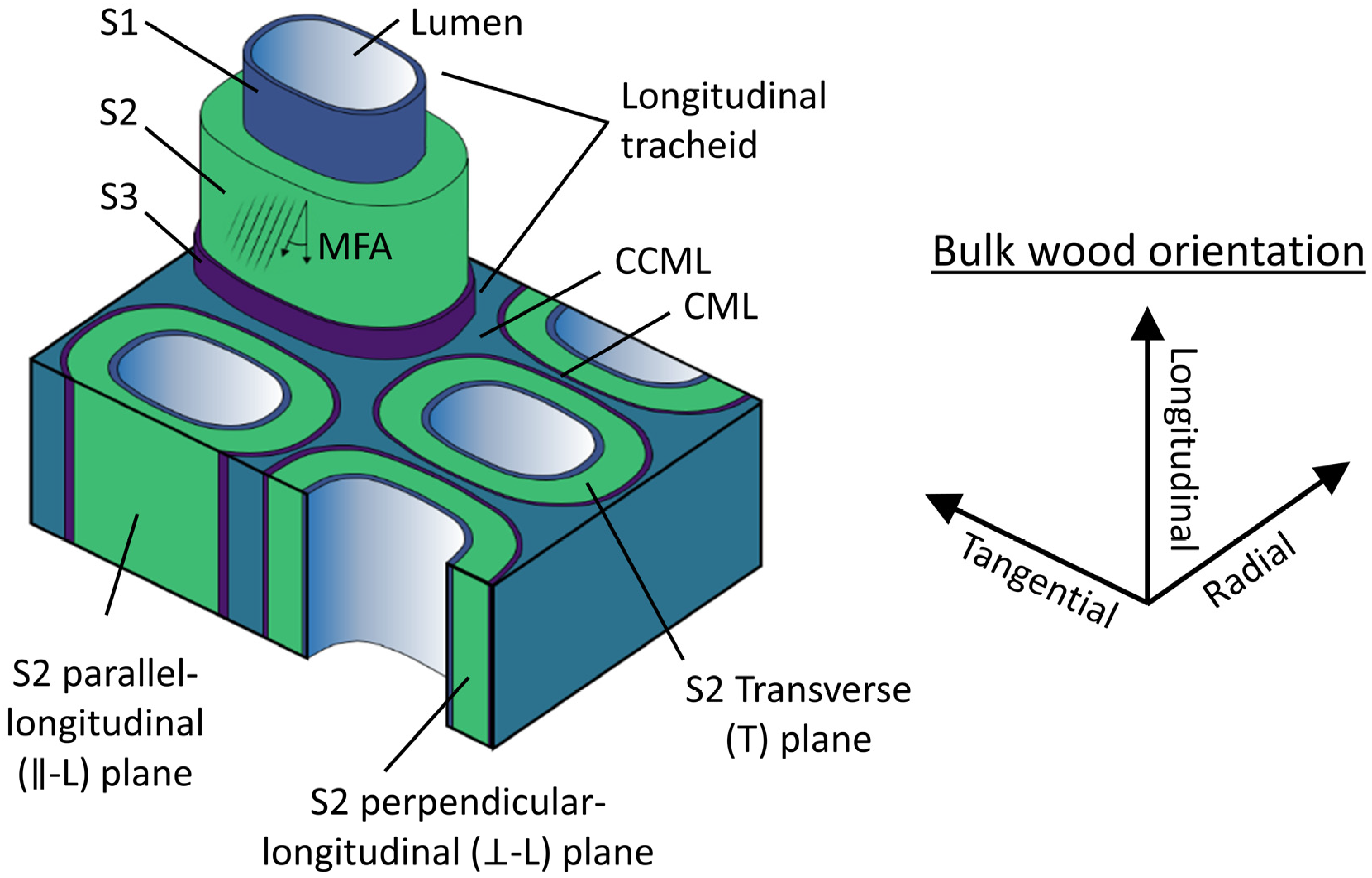
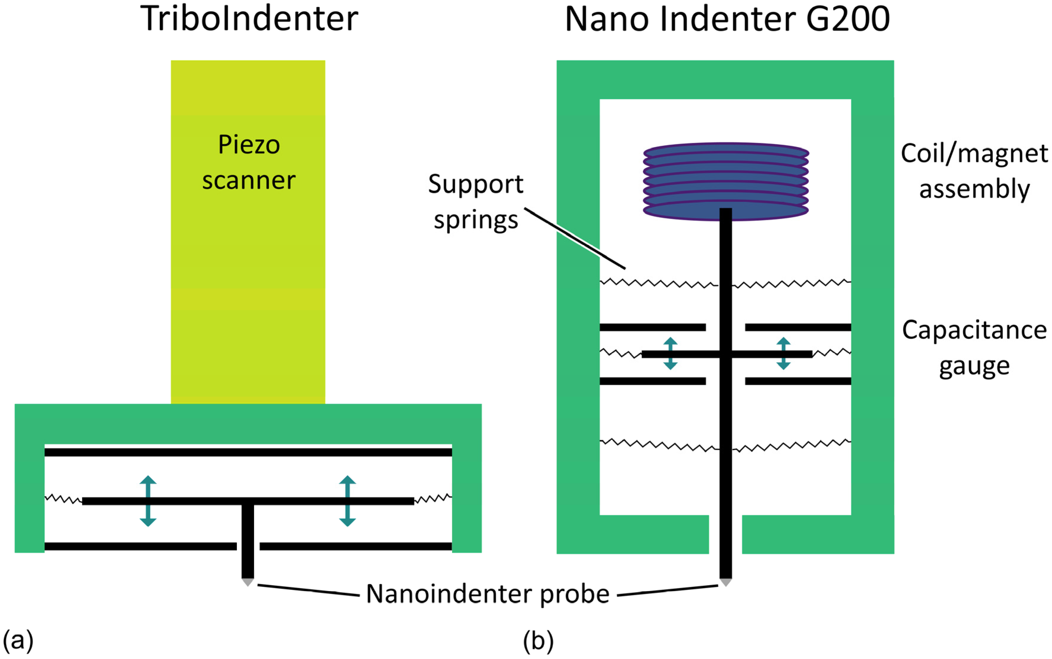
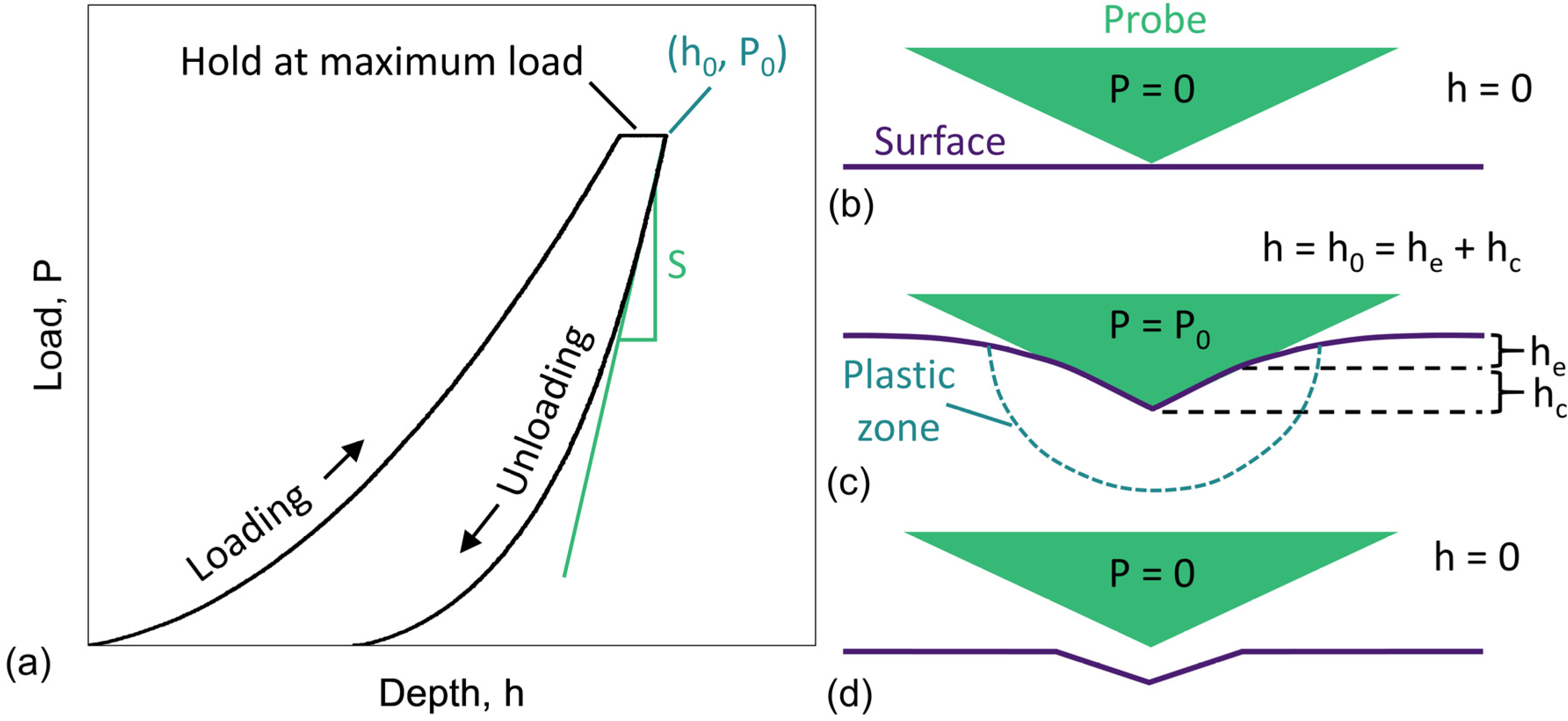
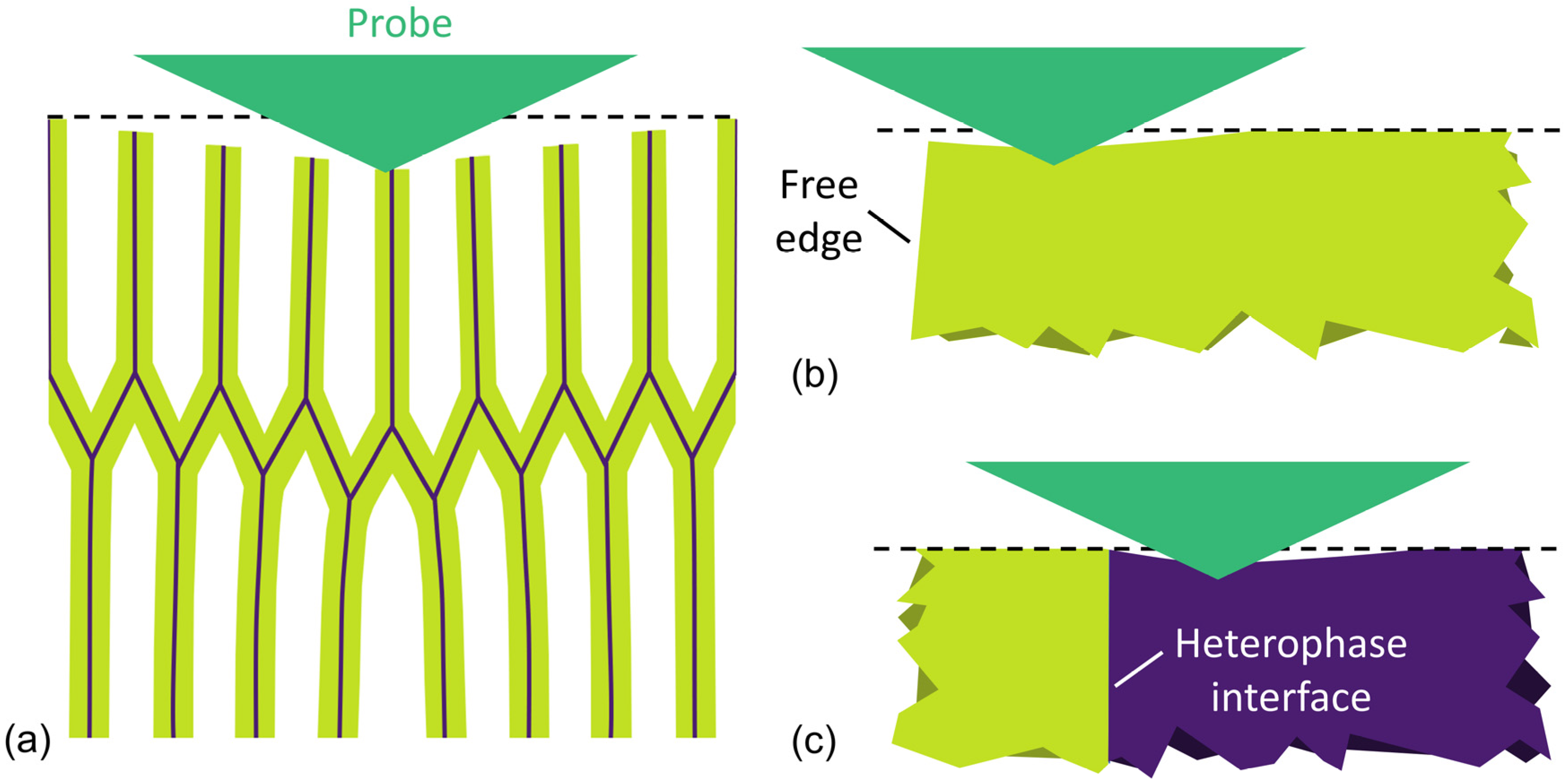
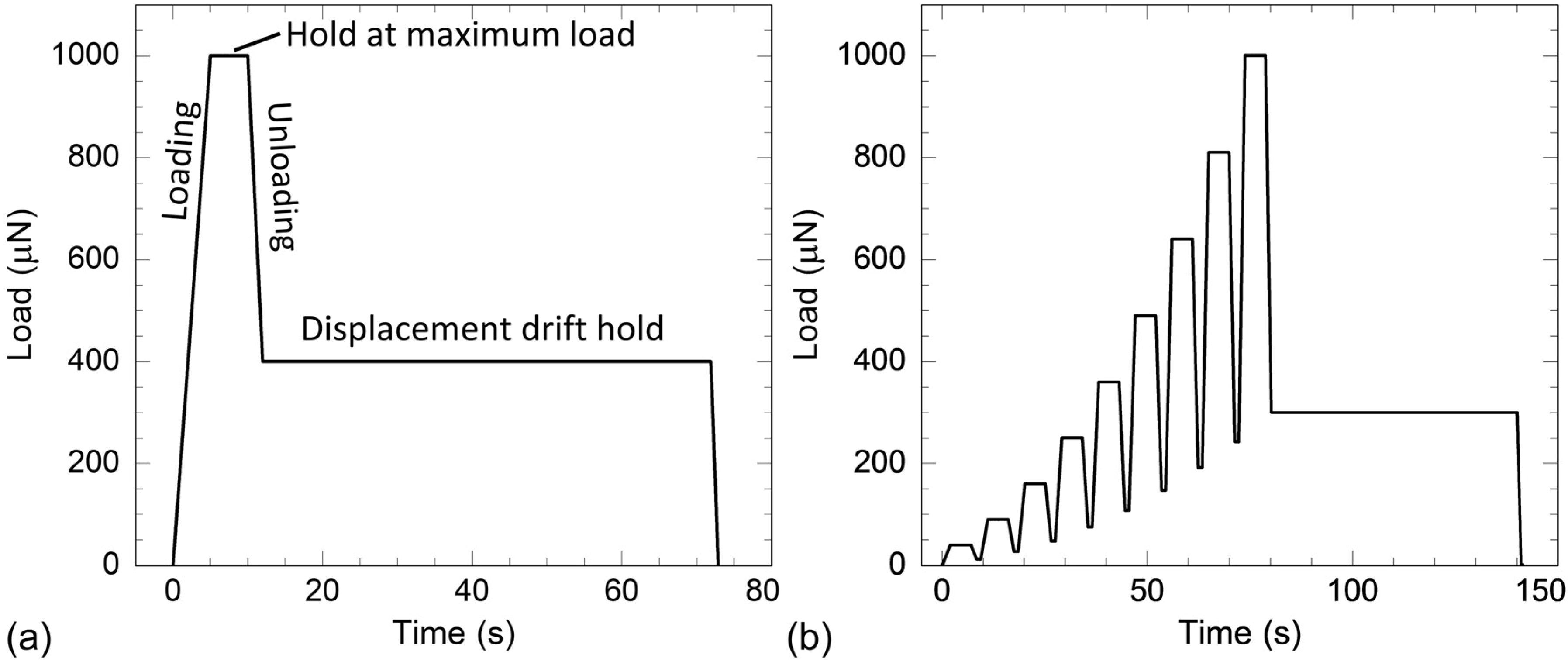
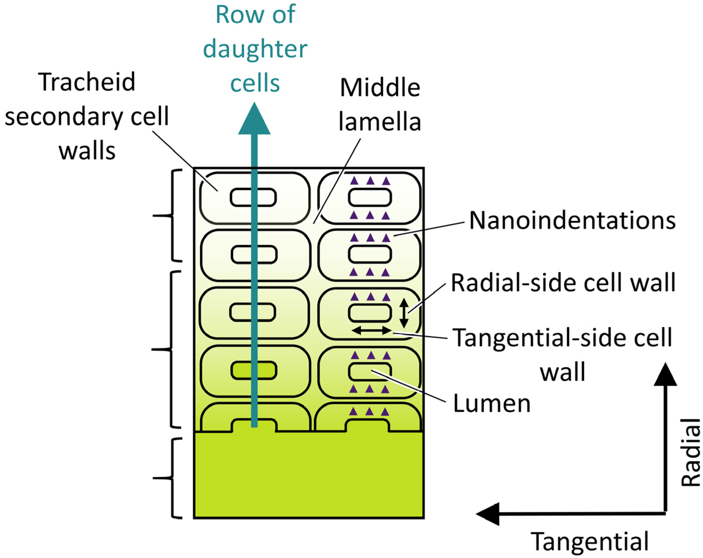
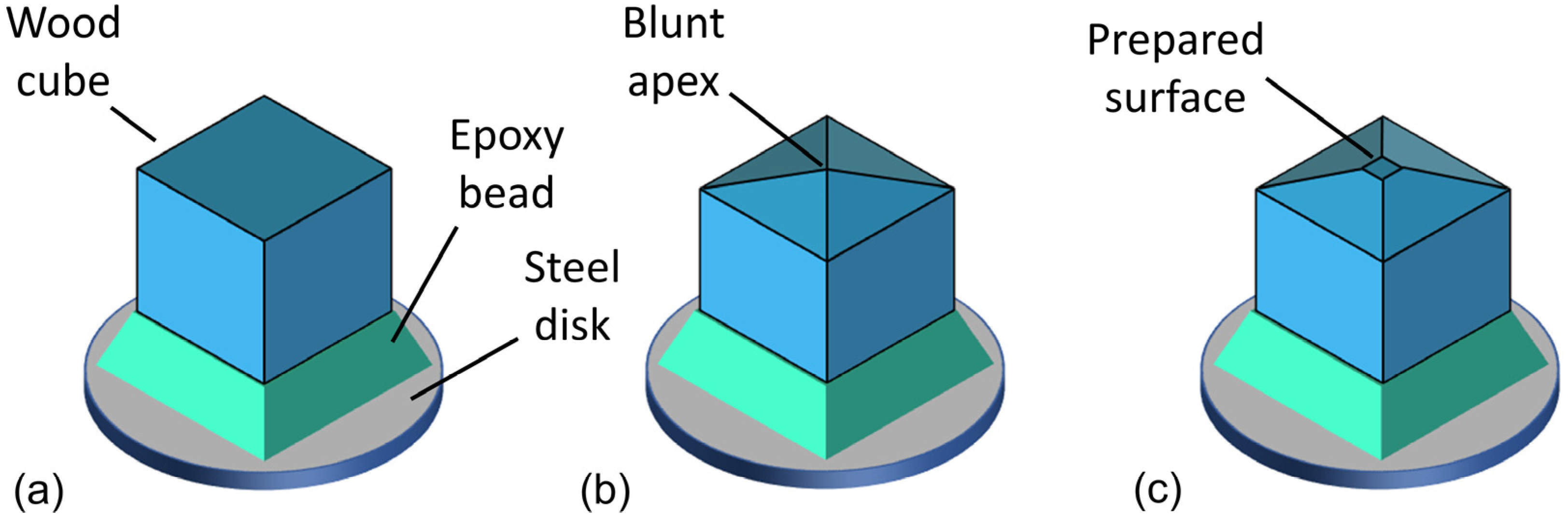
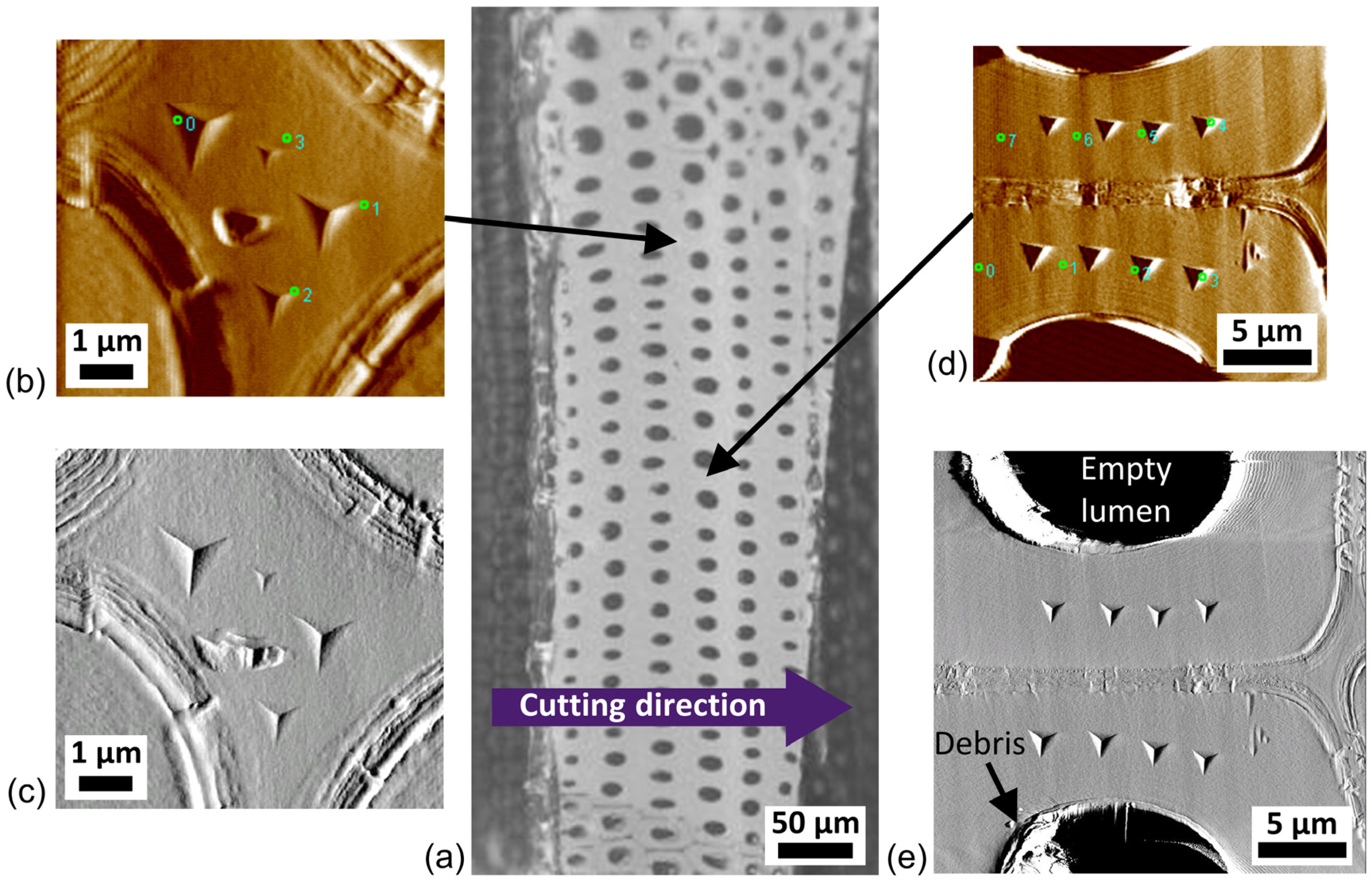
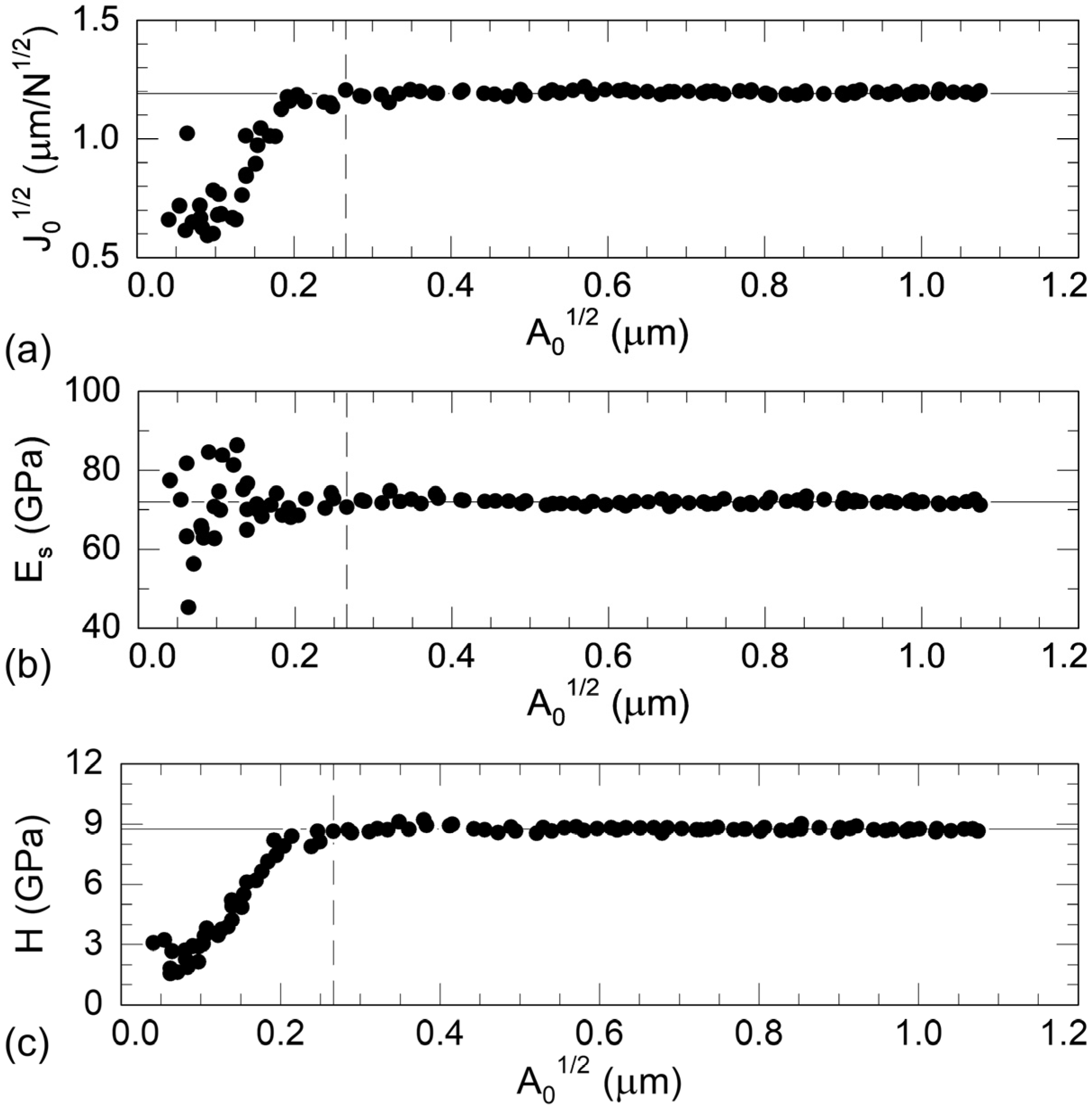
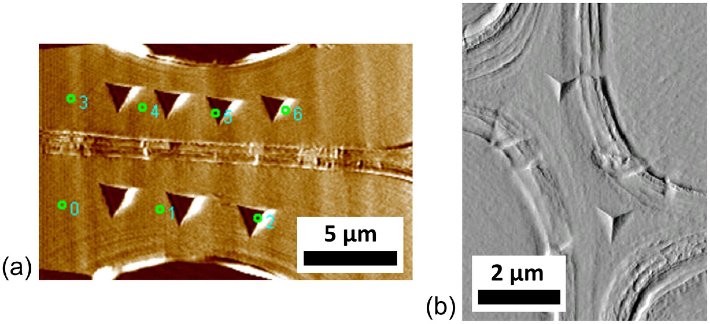
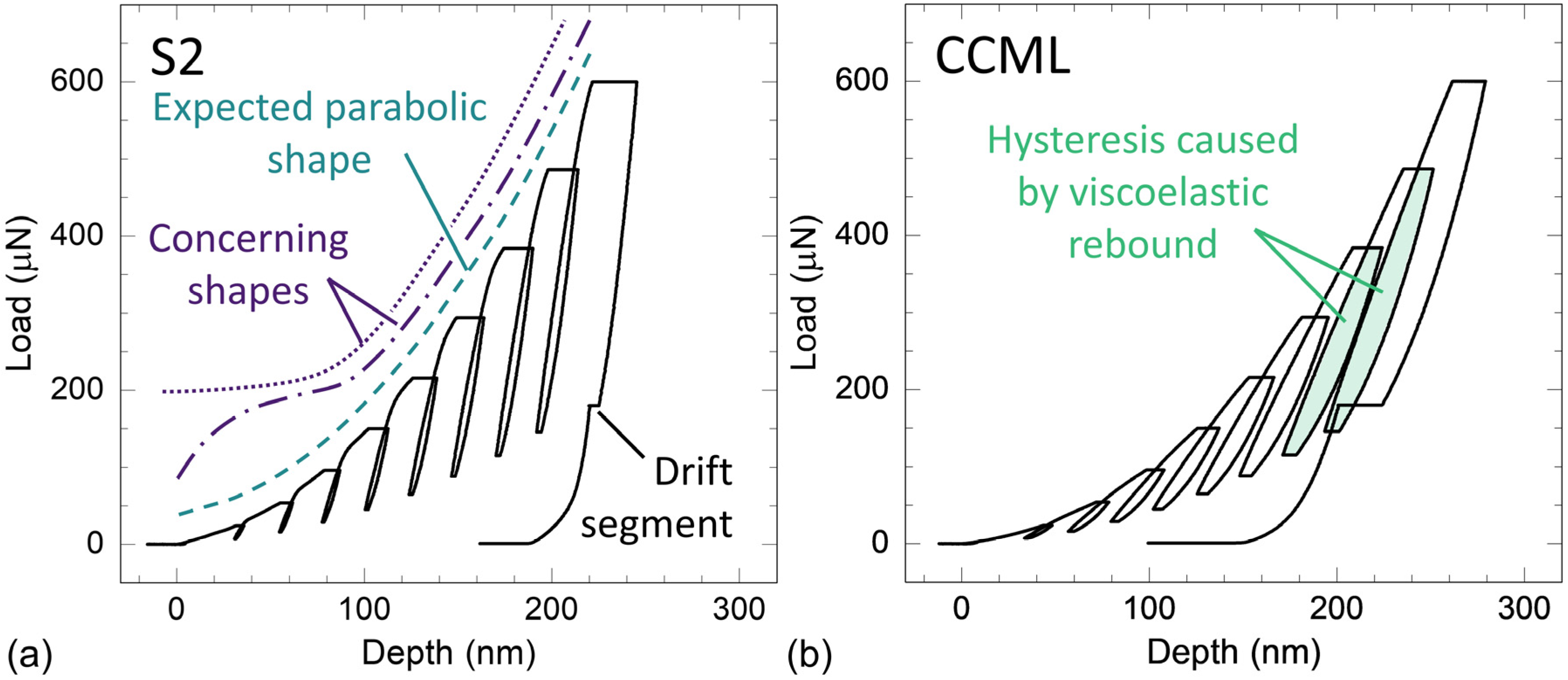
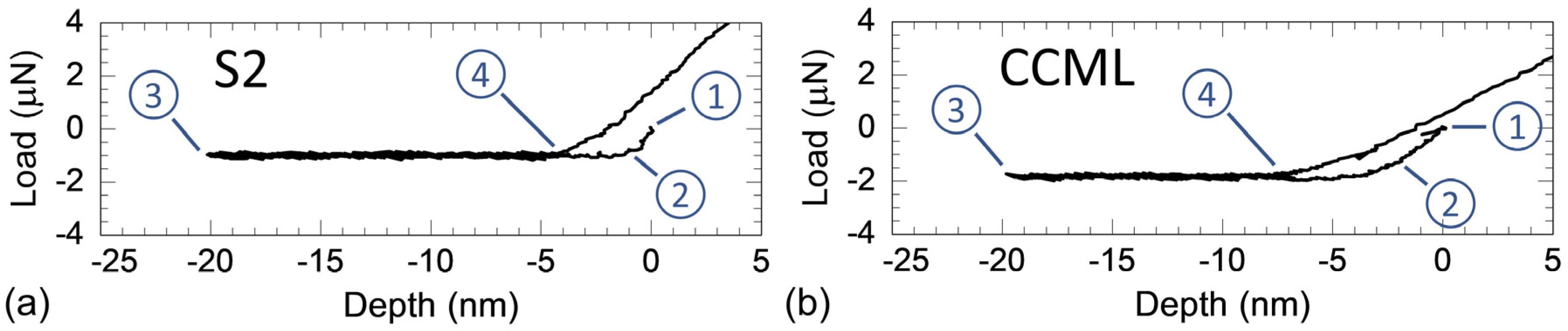
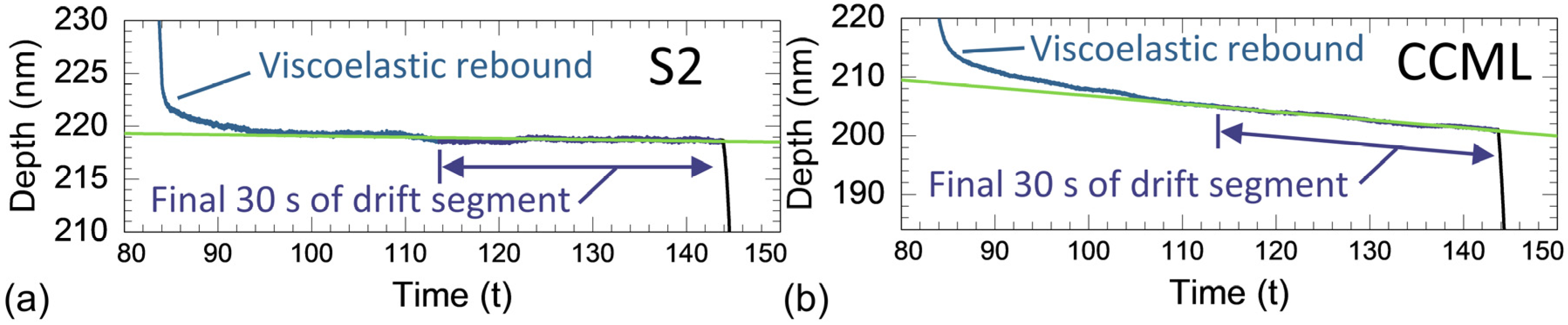
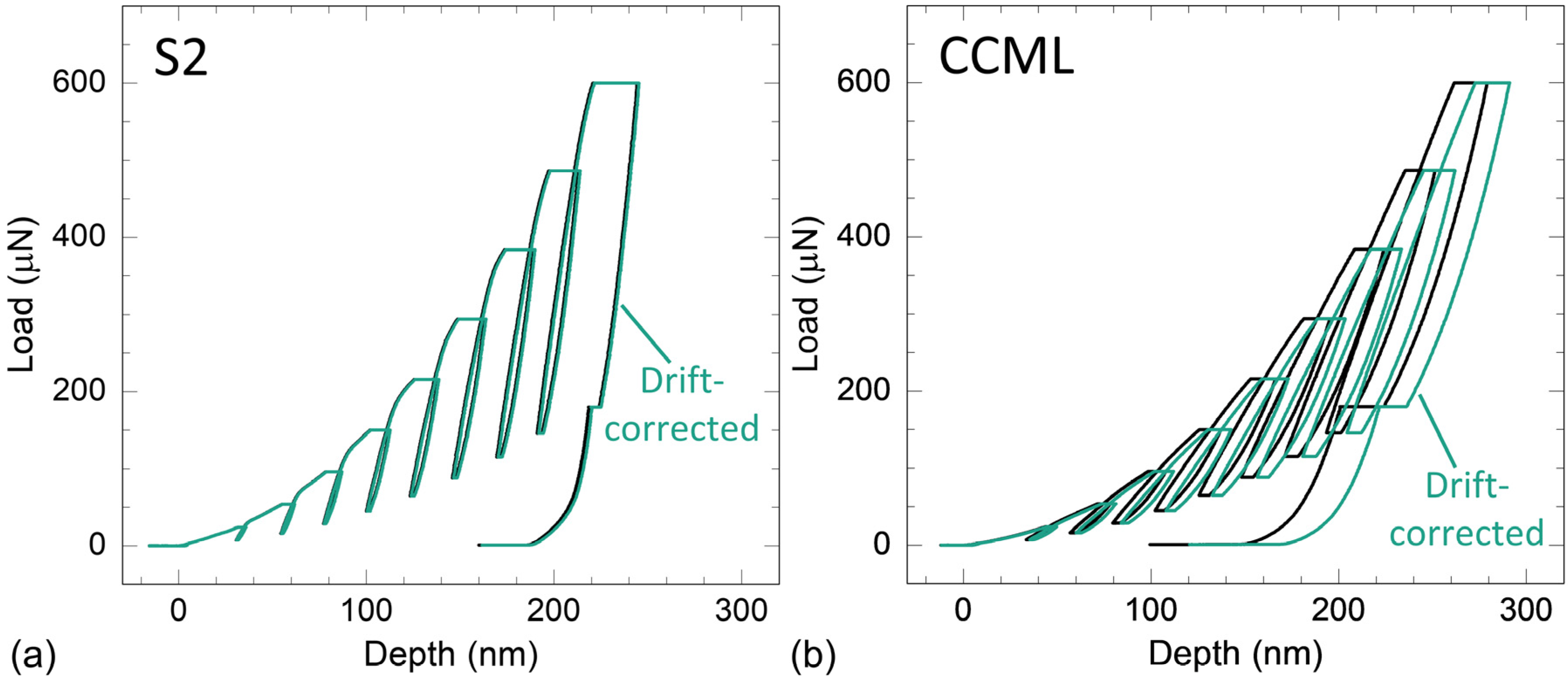
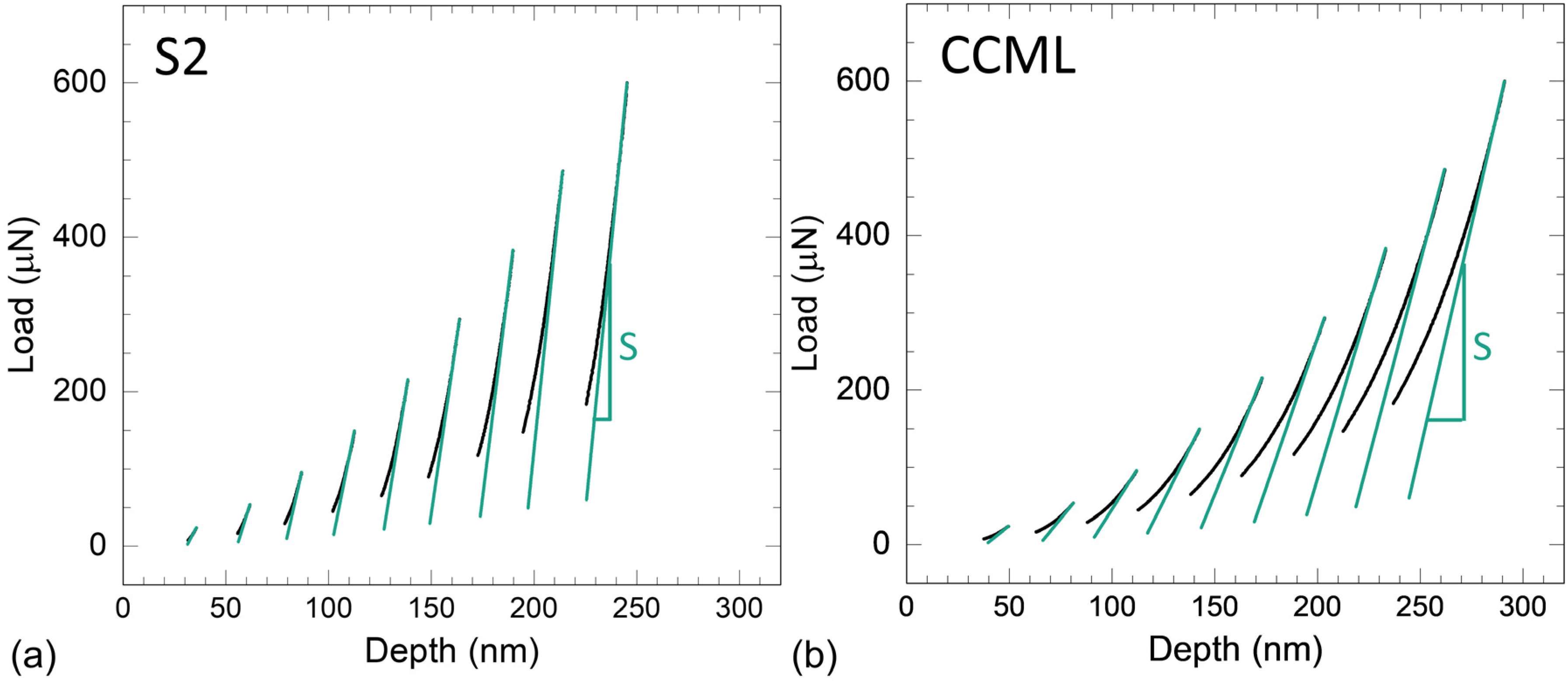
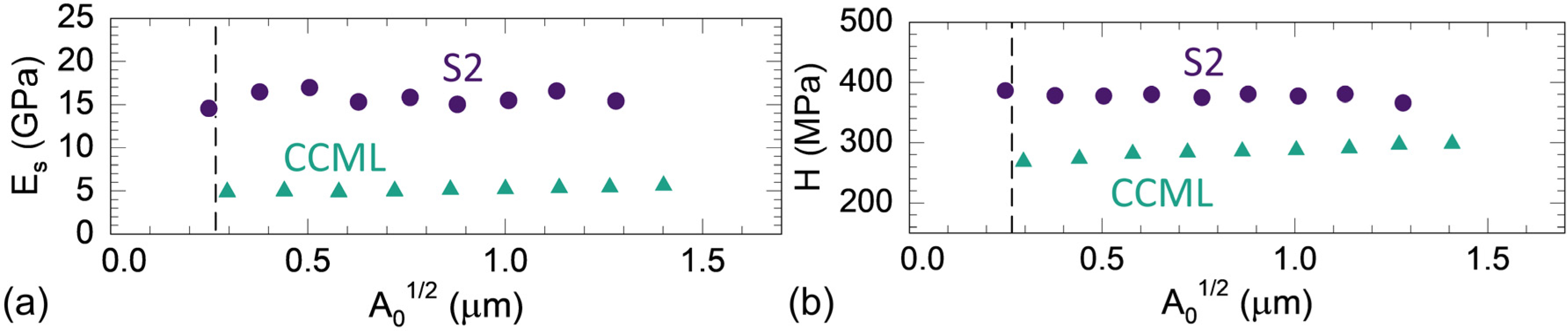
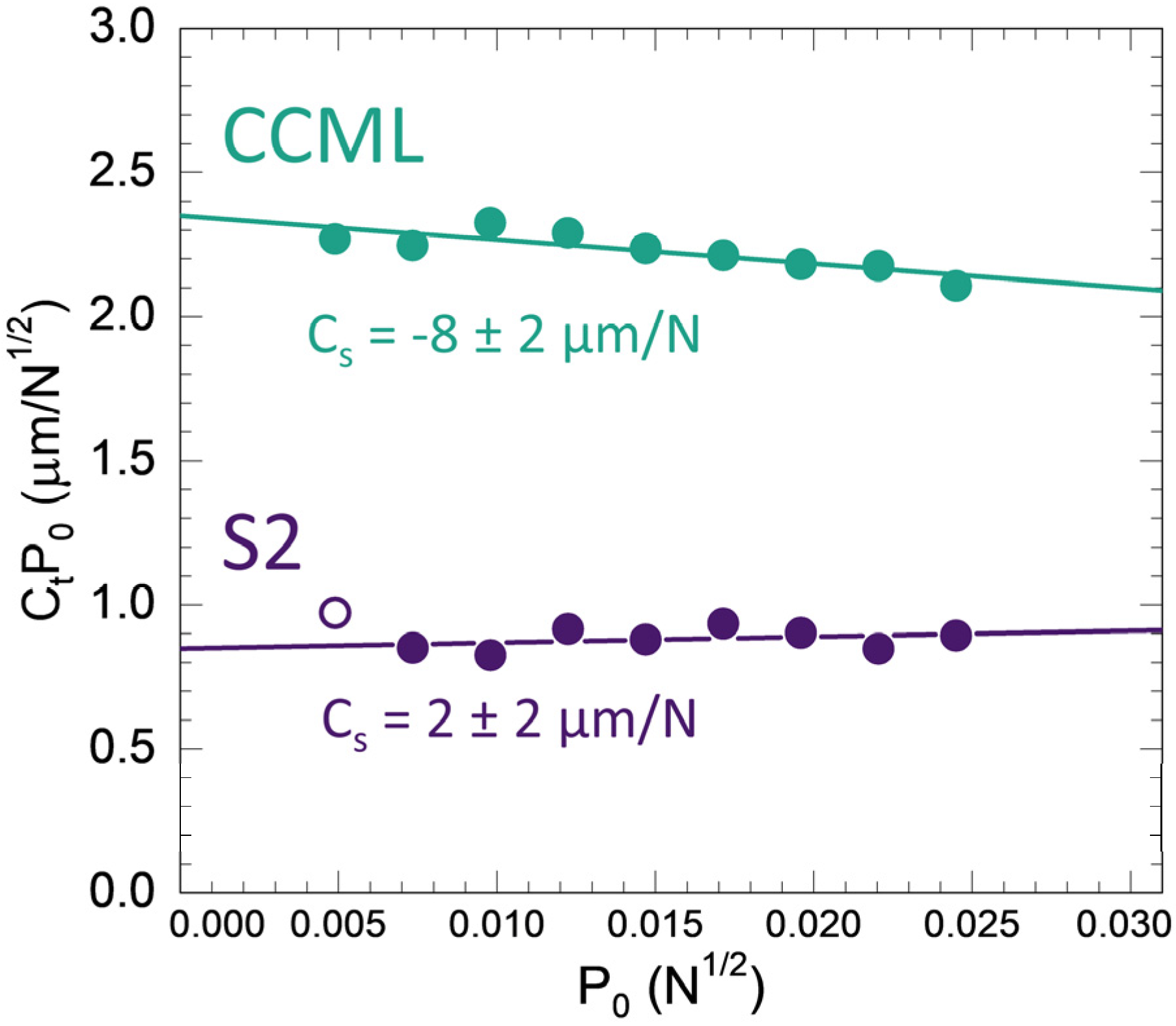
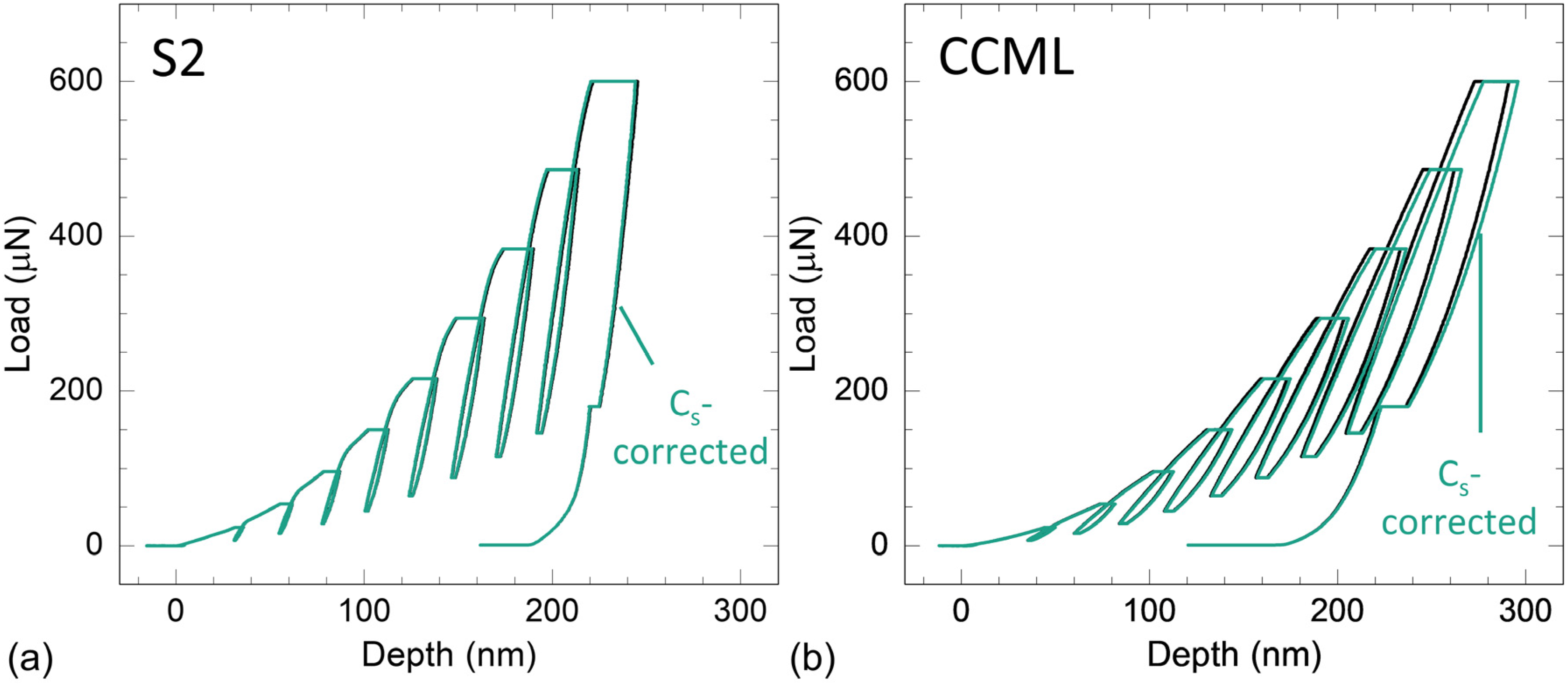
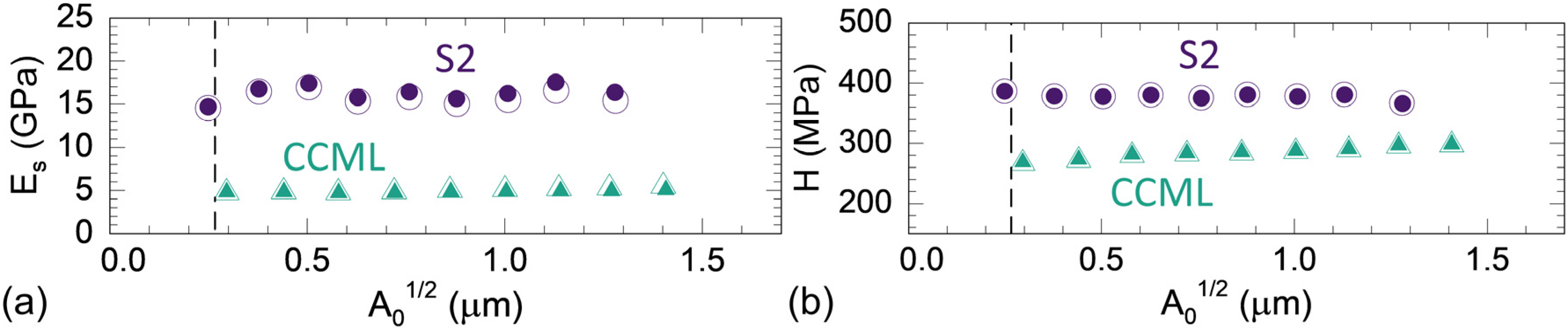
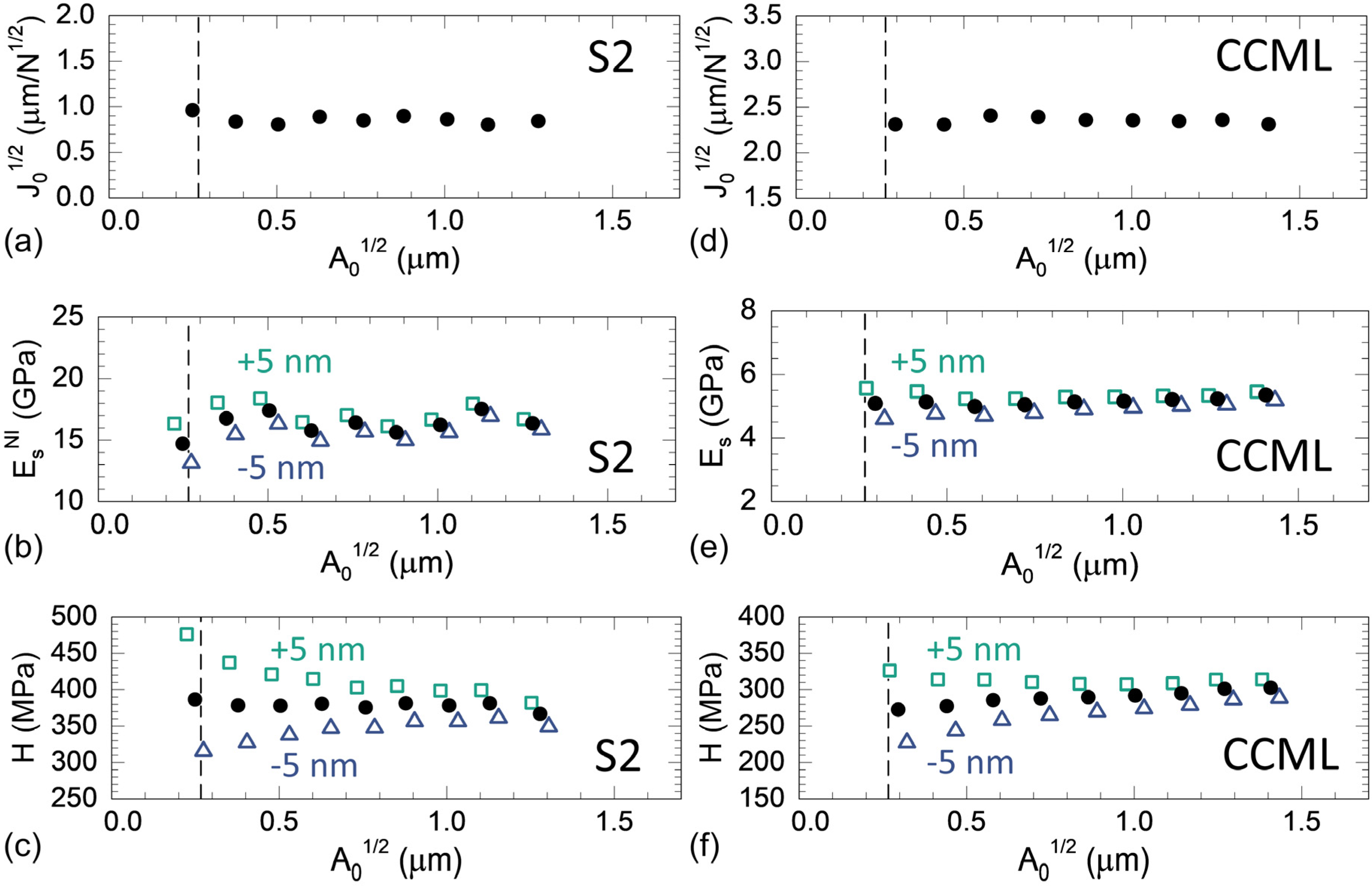
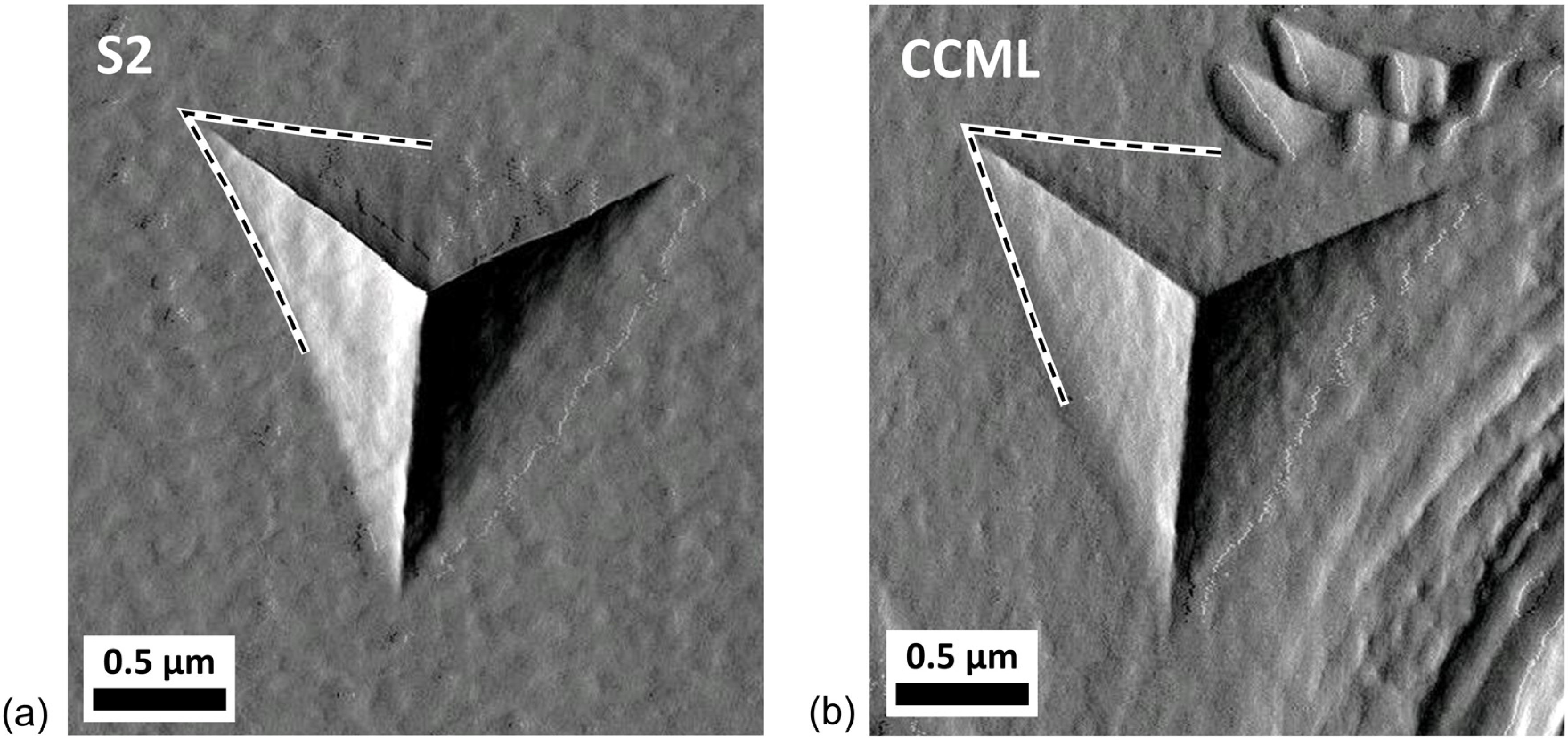
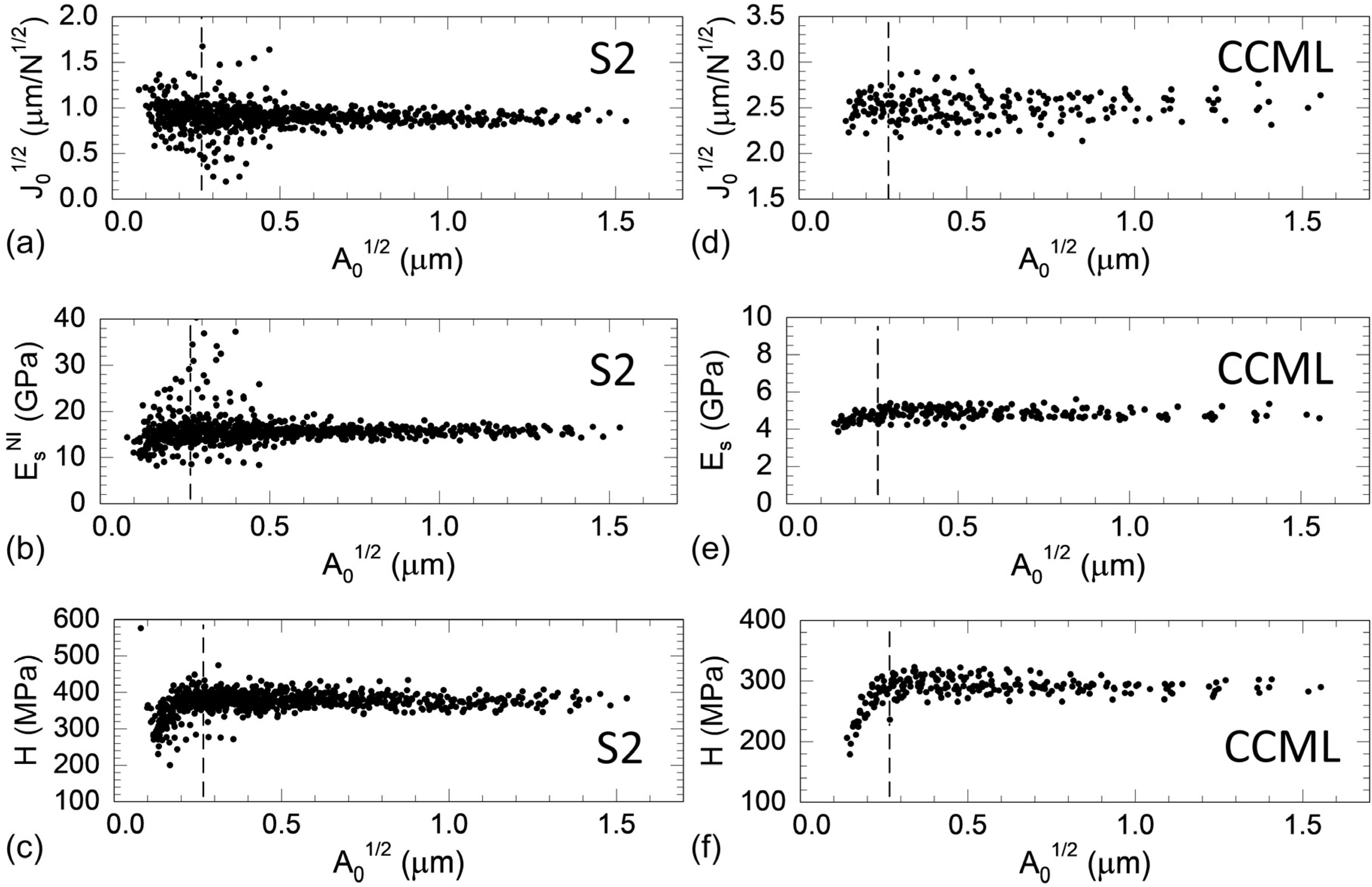
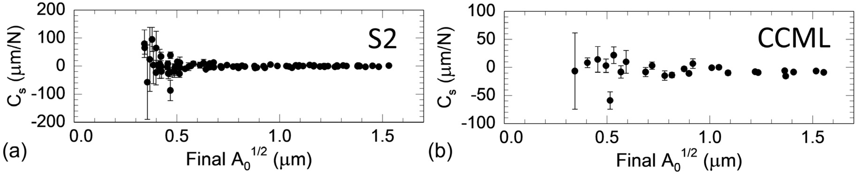
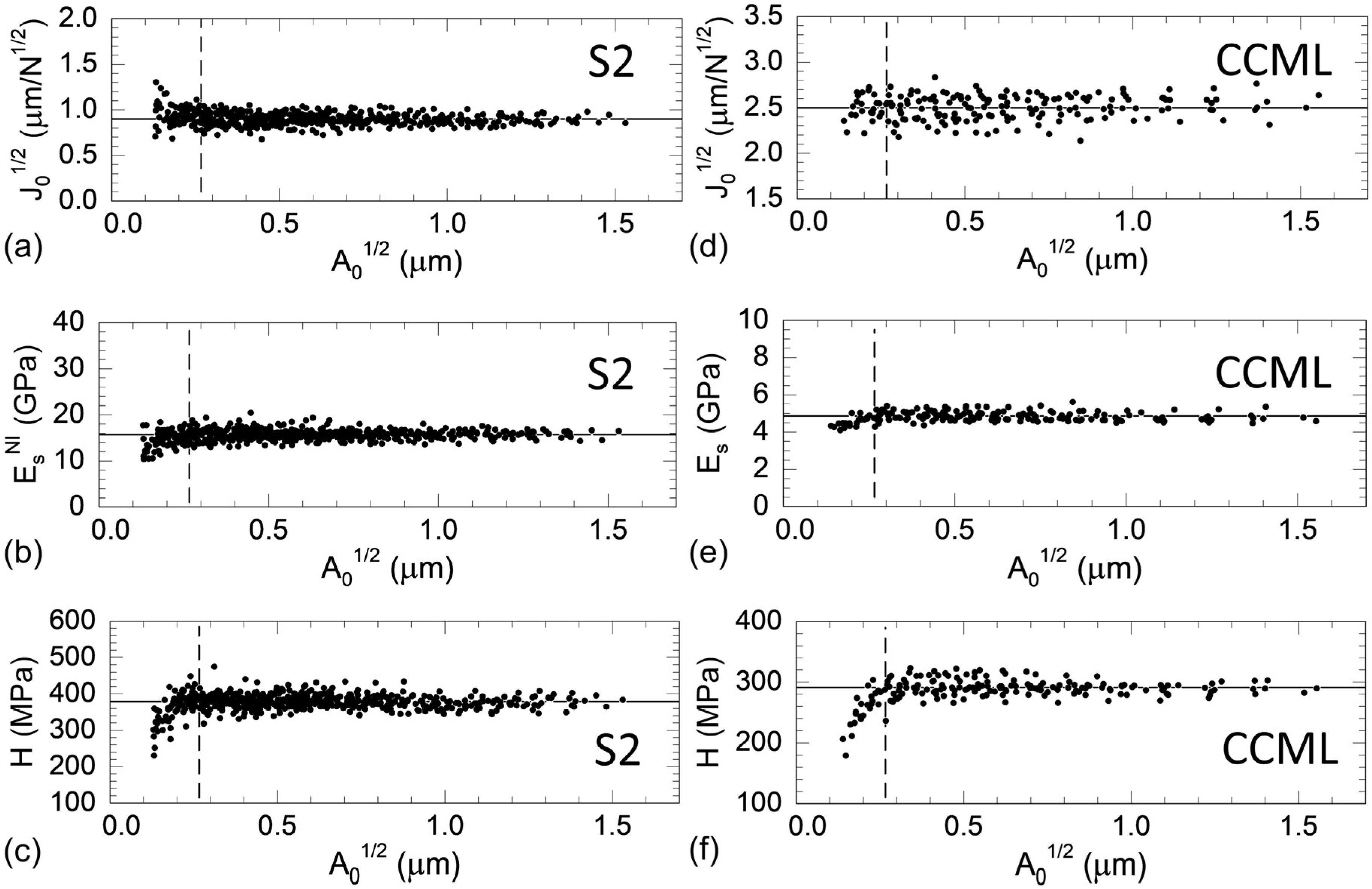
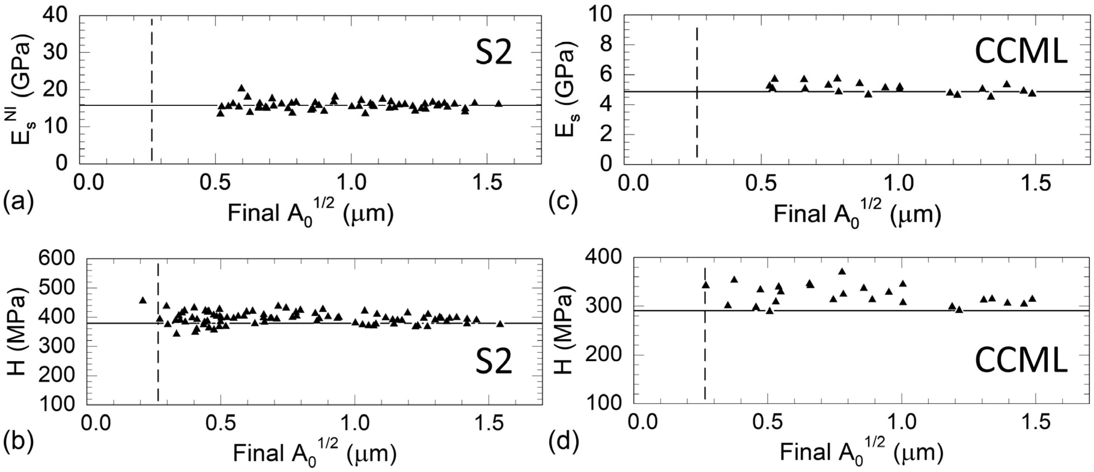
Table 1.
Segment times for each of the nine loading cycles of the multiload load function shown in Figure 5b.
Table 1.
Segment times for each of the nine loading cycles of the multiload load function shown in Figure 5b.
| Loading Cycle | Loading Segment (s) | Hold at P0 Segment (s) | Unloading Segment (s) | Hold at 30% P0 Segment (s) |
|---|---|---|---|---|
| 1 | 2.00 | 5 | 1.4 | 1 |
| 2 | 1.73 | 5 | 1.4 | 1 |
| 3 | 1.66 | 5 | 1.4 | 1 |
| 4 | 1.62 | 5 | 1.4 | 1 |
| 5 | 1.58 | 5 | 1.4 | 1 |
| 6 | 1.56 | 5 | 1.4 | 1 |
| 7 | 1.54 | 5 | 1.4 | 1 |
| 8 | 1.53 | 5 | 1.4 | 1 |
| 9 | 1.51 | 5 | 1.4 | 1 |
Table 2.
Nanoindentation elastic modulus (Es) and hardness (H) results binned into groups by their final nanoindentation sizes, as defined by the square root of their final contact area (Final A01/2).
Table 2.
Nanoindentation elastic modulus (Es) and hardness (H) results binned into groups by their final nanoindentation sizes, as defined by the square root of their final contact area (Final A01/2).
| S2 | ||||||||||
| Final A01/2 Range | Number of Unloading Segments 3 | Es | H | |||||||
| Ave 4 | Std 5 | Ste 6 | Ave | Std | Ste | |||||
| Bin | (μm) | N 1 | n 2 | (GPa) | (GPa) | (GPa) | (MPa) | (MPa) | (MPa) | |
| 1 | 0.33–0.5 | 25 | 100 | 3 to 5 | 18.9 | 11.0 | 1.15 | 376 | 28 | 3 |
| 2 | 0.5–0.75 | 20 | 128 | 5 to 7 | 15.7 | 1.7 | 0.15 | 375 | 19 | 2 |
| 3 | 0.75–1.0 | 12 | 88 | 7 to 8 | 15.6 | 1.2 | 0.12 | 391 | 21 | 2 |
| 4 | 1.0–1.25 | 13 | 112 | 8 | 15.9 | 0.8 | 0.08 | 381 | 17 | 2 |
| 5 | 1.25–1.53 | 15 | 129 | 8 to 9 | 15.7 | 0.8 | 0.07 | 375 | 15 | 1 |
| CCML | ||||||||||
| Final A01/2 Range | Number of Unloading Segments | Es | H | |||||||
| Ave | Std | Ste | Ave | Std | Ste | |||||
| Bin | (μm) | N | n | (GPa) | (GPa) | (GPa) | (MPa) | (MPa) | (MPa) | |
| 1 | 0.31–0.5 | 5 | 18 | 3 to 5 | 5.1 | 0.2 | 0.04 | 305 | 6 | 2 |
| 2 | 0.5–0.75 | 6 | 37 | 5 to 7 | 4.9 | 0.3 | 0.06 | 300 | 14 | 2 |
| 3 | 0.75–1.0 | 6 | 45 | 7 to 8 | 5.0 | 0.2 | 0.04 | 294 | 11 | 2 |
| 4 | 1.0–1.25 | 4 | 33 | 8 to 9 | 4.7 | 0.2 | 0.03 | 286 | 12 | 2 |
| 5 | 1.25–1.58 | 5 | 45 | 9 | 4.8 | 0.2 | 0.04 | 284 | 11 | 2 |
1 N—number of multiload nanoindentations in the bin. 2 n—number of unloading segments in the bin that met the A01/2 > 0.266 μm size criteria. 3 Number of unloading segments—Range for the number of unloading segments that met the A01/2 > 0.266 μm size criteria for the multiload nanoindentations within the bin. 4 Ave—Average. 5 Std—Standard deviation. 6 Ste—Standard error.
Publisher’s Note: MDPI stays neutral with regard to jurisdictional claims in published maps and institutional affiliations. |
© 2021 by the authors. Licensee MDPI, Basel, Switzerland. This article is an open access article distributed under the terms and conditions of the Creative Commons Attribution (CC BY) license (https://creativecommons.org/licenses/by/4.0/).
Share and Cite
MDPI and ACS Style
Jakes, J.E.; Stone, D.S. Best Practices for Quasistatic Berkovich Nanoindentation of Wood Cell Walls. Forests 2021, 12, 1696. https://0-doi-org.brum.beds.ac.uk/10.3390/f12121696
AMA Style
Jakes JE, Stone DS. Best Practices for Quasistatic Berkovich Nanoindentation of Wood Cell Walls. Forests. 2021; 12(12):1696. https://0-doi-org.brum.beds.ac.uk/10.3390/f12121696
Chicago/Turabian StyleJakes, Joseph E., and Donald S. Stone. 2021. "Best Practices for Quasistatic Berkovich Nanoindentation of Wood Cell Walls" Forests 12, no. 12: 1696. https://0-doi-org.brum.beds.ac.uk/10.3390/f12121696
Note that from the first issue of 2016, this journal uses article numbers instead of page numbers. See further details here.