Spatial Agglomeration of China’s Forest Products Manufacturing Industry: Measurement, Characteristics and Determinants

Abstract

China’s forest products manufacturing industry is experiencing the dual pressure of forest protection policies and wood scarcity and, therefore, it is of great significance to reveal the spatial agglomeration characteristics and evolution drivers of this industry to enhance its sustainable development. Based on the perspective of large-scale agglomeration in a continuous space, in this study, we used the spatial Gini coefficient and standard deviation ellipse method to investigate the spatial agglomeration degree and location distribution characteristics of China’s forest products manufacturing industry, and we used exploratory spatial data analysis to investigate its spatial agglomeration pattern. The results show that: (1) From 1988 to 2018, the degree of spatial agglomeration of China’s forest products manufacturing industry was relatively low, and the industry was characterized by a very pronounced imbalance in its spatial distribution. (2) The industry has a very clear core–periphery structure, the spatial distribution exhibits a “northeast-southwest” pattern, and the barycenter of the industrial distribution has tended to move south. (3) The industry mainly has a high–high and low–low spatial agglomeration pattern. The provinces with high–high agglomeration are few and concentrated in the southeast coastal area. (4) The spatial agglomeration and evolution characteristics of China’s forest products manufacturing industry may be simultaneously affected by forest protection policies, sources of raw materials, international trade and the degree of marketization. In the future, China’s forest products manufacturing industry should further increase the level of spatial agglomeration to fully realize the economies of scale.

1. Introduction

The forest products manufacturing industry is an important part of China’s national economy and plays a key role in providing raw materials for production, promoting economic growth and increasing employment [1]. China has become the world’s largest country in the forest products trade, as well as the world’s largest producer and consumer of forest products [2]. In 2018, China’s total imports and exports of forest products reached USD 83.7 billion and USD 81.6 billion, respectively, a total value of USD 165.3 billion [3]. According to statistics from the National Forestry and Grassland Administration (NFGA), the import trade volume of logs, wood pulp and paper products accounted for 56.2% of China’s total forest product imports, while wooden furniture and plywood accounted for 66.8% of the total forest product exports. However, China’s forest products manufacturing industry is facing several problems: it is large but weak, and there is still a large gap in product quality and added value compared with developed countries [4]. Furthermore, more than 50% of China’s forest products manufacturing industry is dependent on imported raw materials, and almost 40% of product sales are dependent on overseas markets. The forest product export market is mainly concentrated in a few countries, such as the United States, Japan and members of the European Union [5]. In 2017, the Chinese government announced the full implementation of the prohibition of the commercial cutting of natural forests in the country, which further aggravated the imbalance between supply and demand of Chinese timber [2]. In order to enhance the international competitiveness and sustainable development ability of the forest products manufacturing industry, the Chinese government proposed to optimize the layout of wood processing, furniture, paper and other industries, and give play to the agglomeration effect of key industries and competitive advantages of regional industries in the “13th Five-Year Forestry Development Plan (2016–2020)”. As a typical resource-based industry, it is a topic worthy of in-depth study to accurately grasp the spatial agglomeration characteristics and determinants of the forest products manufacturing industry in China.

The role of industrial spatial agglomeration in economic and regional development has long been a focus of academics and policy makers [6,7]. In terms of economic policy, industrial spatial agglomeration inevitably arises during the industrialization process in developing countries, and it is also an important mechanism for the formation of growth poles or growth zones in regional economic development [8,9]. From the perspective of theoretical development, many related studies have recognized that the concept of sustainable development requires the coordinated development of ecology and the economy [10], and industrial spatial agglomeration can promote ecologically sustainable development [11]. Similar to environmental sustainability, spatial economic sustainability reflects the spatial structure and dynamics of regional economic production and consumption activities. Spatial economic sustainability depends on the pattern (agglomeration or diffusion pattern) and degree of economic agglomeration, both of which significantly affect the level of negative environmental externalities [12]. Although some studies have emphasized the importance of sustainable development in the forest products manufacturing industry, the systematic analysis of this issue from a spatial perspective is still lacking [13]. In addition, the characteristics of spatial agglomeration evolution in forest products manufacturing have not been fully explored, because previous studies have focused on either the overall manufacturing industry [14] or the impact of spatial agglomeration on forest products trade [1,15]. What is the degree of spatial agglomeration in China’s forest products manufacturing industry? Where does spatial agglomeration occur? How have the characteristics of spatial agglomeration changed? What are the determinants of the spatial agglomeration location distribution? Answering these questions will help to provide a scientific basis for the formulation of sustainable development policies for China’s forest products manufacturing industry.

Since the 1980s, the spatial agglomeration of manufacturing has gradually received increasing attention from scholars in the fields of industrial, spatial and regional economics. Industrial spatial agglomeration is usually defined as the geographical concentration of companies and institutions with common or complementary properties in a specific field [16]. As a global economic phenomenon, industrial spatial agglomeration is also considered the most prominent geographical feature of economic activities [17]. The agglomeration economy originated from the exploration of industrial agglomeration by economist Marshall (1895). Labor market sharing, intermediate product trade and knowledge information spillover were determined to be important forces in promoting the formation of industrial agglomeration, which laid the foundation for the construction of the industrial agglomeration theory [18]. After that, economists in different periods further developed the theory of industrial spatial agglomeration from the perspectives of spatial competition [19], the external economy [20], polarization effects [21], resource scarcity [22], etc. In the 1990s, with the emergence of the new economic geography theory, a new direction opened up for exploring the formation mechanism of industrial spatial agglomeration. Under the framework of the new economic geography, economist Krugman (1991) revealed how transportation costs, factor flows and economies of scale affect the spatial agglomeration of economic activities through market transmission mechanisms, which solved problems that could not be answered by the traditional location advantage theory [23,24]. Since entering the 21st century, with the active participation of developing countries in the division of labor in the global manufacturing value chain, scholars have focused on the trends and determinants of industrial spatial agglomeration [25,26,27,28], the relationship between spatial agglomeration and economic development [29,30] and the impact of spatial agglomeration on environmental pollution [31,32,33] and productivity [34,35,36]. Many studies have confirmed the positive effect of industrial spatial agglomeration on economic development, productivity and technological innovation, but the degree of influence has been found to vary among different regions [37,38]. However, other studies have reported that excessive agglomeration has negative effects, such as lock-in effects on the industry, rising fixed costs, increasing market barriers and a deteriorating ecological environment [39,40,41]. Thus, the results of existing studies provide inconsistent evidence on the economic impact of industrial spatial agglomeration. Because of these discrepancies in theoretical and empirical results, despite more than 100 years of research, there is still much debate among scholars over the causes of industrial agglomeration; similar controversies about the measurement method of industrial agglomeration are also prevalent [42]. For example, disagreement arises over whether to use enterprise-level data or macro statistical data for research and whether to use traditional indicators (location entropy, Gini coefficient, etc.) or emerging indicators (Ellison–Glaeser localization index (EG index), etc.) [42,43]. Some researchers argue that traditional indicators do not account for the impact of industrial structure [44], but emerging indicators cannot be used for dynamic measurements over a long time span. In addition, enterprise-level data are rarely used because they are difficult to collect and process [45,46]. From a practical point of view, both types of indicators are currently widely used by researchers, and the measurement methods depend on the type of data used in the research. For example, the spatial agglomeration of China’s manufacturing industry was measured using the Gini coefficient and the EG index by He and Wang [47] and He et al. [48], respectively. Generally speaking, although the phenomenon of spatial agglomeration is an extensively researched issue in academia, inconsistencies in the study areas and the methods of agglomeration measurement have led to great academic controversy over the economic spillover effects of spatial agglomeration.

In addition, similar academic disputes are also pervasive in the field of forest products manufacturing. Although a few studies have analyzed the spatial agglomeration of China’s forest products manufacturing industry and its sub-industries, they have yielded conflicting results on the characteristics of this phenomenon [1,15,49,50,51,52,53,54]. For example, in these studies, the agglomeration of China’s wood processing industry has been characterized as moderate [51,53], high [49] and excessive [52]. The spatial agglomeration of the furniture manufacturing industry was concluded to be low [54] and moderate [51]. The spatial agglomeration of the paper industry has also been categorized as low [51] and moderate [50]. In most of these studies, scholars used only one method to measure the degree of spatial agglomeration of China’s forest products manufacturing industry. However, a single research perspective is insufficient to accurately describe the spatial agglomeration characteristics of this industry in China. These phenomena indicate that, compared with the spatial agglomeration effect of the industry, its spatial agglomeration characteristics have not been fully explored and evaluated. Previous studies provide a valuable research basis for this article, but they have some limitations: on the one hand, previous studies have overemphasized the role of micro data, so the scope of research has been limited to the analysis of the short-term characteristics of the spatial agglomeration of the forest products manufacturing industry; on the other hand, the relevant literature includes almost no in-depth discussion on the reasons for the evolution of industrial spatial agglomeration, and there is still confusion in academic circles on how to realize the sustainable development of China’s forest products manufacturing industry. In contrast to previous studies, the research in this paper combined multiple methods: the spatial Gini coefficient, standard deviation ellipse and exploratory spatial data analysis. In addition, the research was based on provincial-level data that can reflect the development status of China’s forest product manufacturing and its sub-industries. Finally, the spatial agglomeration of China’s forest products manufacturing industry and its evolution were carefully investigated from the perspectives of the spatial agglomeration degree, spatial location distribution characteristics and spatial agglomeration pattern. This study may help to solve the academic controversy in related research, encourage Chinese local governments to re-examine local economic development planning and industrial policies and provide a decision-making reference for the optimization of the spatial layout of the forest products manufacturing industry.

The remainder of the paper is structured as follows. Section 2 describes the research methods and data sets. In Section 3, firstly, the industrial spatial distribution of China’s forest products manufacturing industry is described, and the spatial agglomeration degree of the industry is analyzed based on the spatial Gini coefficient. Secondly, the evolution of the spatial agglomeration of the forest products manufacturing industry is analyzed, for which the standard deviation ellipse method is used; then, the local Moran’s I index of spatial econometrics is used to identify the spatial agglomeration areas of forest products manufacturing in different periods. Section 4 discusses the theoretical and policy significance, limitations and future research directions of this paper. Finally, the main conclusions of this study are summarized in Section 5.

2. Materials and Methods

2.1. Research Methods

In previous literature, the measurement methods of industrial spatial agglomeration include the Hoover index, Gini coefficient, Herfindahl index, Theil index, Entropy index and EG index, among others [43,48]. In order to more comprehensively investigate the spatial agglomeration characteristics and evolution trends of China’s forest products manufacturing industry, an empirical analysis was carried out from three perspectives: the degree of industrial agglomeration, spatial location distribution characteristics and the spatial agglomeration pattern. For this purpose, a variety of methods were used: the spatial Gini coefficient, standard deviation ellipse technique and exploratory spatial data analysis. Specifically, the spatial Gini coefficient can measure the spatial agglomeration degree of China’s forest products manufacturing industry, and the standard deviation ellipse technique can accurately characterize the spatial location distribution of the industry. The exploratory spatial data analysis enables the detailed investigation of the spatial agglomeration pattern and its evolutionary trend in China’s forest products manufacturing industry. For the purpose of this paper, these methods cannot be substituted for each other, and each research perspective necessitates a specific research method. For example, the global Moran’s I index can reflect the spatial agglomeration trend of China’s forest products manufacturing industry, but it cannot reflect the spatial agglomeration degree.

2.1.1. Spatial Gini Coefficient

According to a review of the relevant research on China’s forest products manufacturing industry, scholars usually use one of three methods, namely, the EG index, industry concentration ratio or spatial Gini coefficient, to measure the degree of spatial agglomeration of the industry. For example, Li et al. [1,50], Tao et al. [15,49] and Xia and Shen [51,53] applied the EG index, whereas Yang et al. [52] and Zeng and Nie [54] used the industry concentration ratio and spatial Gini coefficient, respectively. The disadvantage of using the EG index is that micro data are difficult to obtain, the research period is short and it is impossible to analyze the spatial agglomeration degree of China’s forest product manufacturing industry from a long-term perspective. For this reason, scholars have chosen 1998–2013 as the research period. Although the industry concentration ratio is simple and intuitive, the number of regions is set subjectively, and the calculation result must have random volatility. The spatial Gini coefficient does not need to rely on micro data, and it uses the geographic distribution of all industries as a benchmark, allowing the spatial agglomeration degree of different industries to be compared in the long term. Compared with the EG index and the industry concentration ratio, it has distinct advantages. The spatial Gini coefficient is also a widely used index in empirical research on manufacturing agglomeration. For example, Krugman (1991) proposed the concept of the spatial Gini coefficient by combining the Lorentz curve with the traditional Gini coefficient when examining the agglomeration degree of the American manufacturing industry [17]. Aiginger and Rossi-Hansberg (2006) used the spatial Gini coefficient to analyze manufacturing agglomeration in the United States and the EU; they found that lower transportation costs increase the degree of manufacturing specialization but reduce the degree of industrial spatial agglomeration [55]. Following the above research approaches, the spatial Gini coefficient was used in this study to measure the spatial agglomeration degree of China’s forest products manufacturing industry. The specific expression of the spatial Gini coefficient is shown in Formula (1) [42,44]:

$$G={\displaystyle \sum _{i=1}^n{{\displaystyle (s_i-x_i)}}^2}$$

(1)

where G is the spatial Gini coefficient (0 ≤ G ≤ 1), S_i represents the proportion of the forest products manufacturing industry of province i in the output value of the national forest products manufacturing industry and x_i represents the proportion of the manufacturing industry of province i in the output value of the national manufacturing industry. The closer the value of the spatial Gini coefficient to 0, the lower the degree of spatial agglomeration of the industry; the closer the value of the spatial Gini coefficient to 1, the higher the degree of spatial agglomeration of the industry. It is emphasized that the spatial Gini coefficient is not only a simplified form of the EG index but also an important part of it. In essence, it accounts for the impact of geographical area on the geographical concentration of industries. It is more accurate than the Herfindahl index in describing the degree of spatial agglomeration. The calculation process of the spatial Gini coefficient can be realized by Stata 16.1 software, and this article provides the corresponding software code (Appendix A). Of course, if readers are interested, it can also be calculated by other software, but it may take more time.

2.1.2. Standard Deviation Ellipse

In this study, the standard deviation ellipse (SDE) method was used to investigate the location characteristics of the spatial agglomeration of China’s forest products manufacturing industry. SDE was first proposed by Lefever (1926) to reveal the spatial distribution range of geographic elements [56], and it is currently widely used in economics, sociology, geography, ecology and other fields. For example, Yang et al. analyzed the change in the trajectory of the SDE barycenter to determine whether port transportation was shifting from Hong Kong, China, to mainland China [57]. Du et al. used SDE to explore the spatial evolution of carbon emissions and the economy in China’s construction industry, and their results indicate that carbon decoupling in the industry showed a certain spatial agglomeration phenomenon [58]. As a typical geospatial statistical analysis tool, SDE can accurately explain the spatial distribution characteristics of research objects, such as the degree of dispersion, the degree of agglomeration and the evolution trend [59]. This method calculates the standard distance of a series of points in major and minor axis directions and produces calculation results in the form of ellipses on the map. The dynamic trend of economic activities can be described more intuitively by the length and direction of the ellipse axis [60,61]. The parameters of SDE usually include its barycenter, the standard deviation of the major and minor axes and the azimuth angle, among other factors [58,60,61], and the details are as follows.

$${\overline{X}}_w=\frac{{\displaystyle \sum _1^n{\omega }_i{x}_i}}{{\displaystyle \sum _1^n{\omega }_i}}{\overline{Y}}_w=\frac{{\displaystyle \sum _1^n{\omega }_i{y}_i}}{{\displaystyle \sum _1^n{\omega }_i}}$$

(2)

$${\sigma }_x=\sqrt{\frac{{\displaystyle \sum _1^n{\left({\omega }_i{\overline{x}}_i\cos \theta -{\omega }_i{\overline{y}}_i\sin \theta \right)}^2}}{{\displaystyle \sum _1^n{\omega }_i^2}}}$$

(3)

$${\sigma }_y=\sqrt{\frac{{\displaystyle \sum _1^n{\left({\omega }_i{\overline{x}}_i\sin \theta -{\omega }_i{\overline{y}}_i\cos \theta \right)}^2}}{{\displaystyle \sum _1^n{\omega }_i^2}}}$$

(4)

$$\tan \theta =\frac{\left({\displaystyle \sum _1^n{\omega }_i^2{\overline{x}}_i^2-{\displaystyle \sum _1^n{\omega }_i^2{\overline{x}}_i^2}}\right)+\sqrt{{\left({\displaystyle \sum _1^n{\omega }_i^2{\overline{x}}_i^2-{\displaystyle \sum _1^n{\omega }_i^2{\overline{y}}_i^2}}\right)}^2+4{\displaystyle \sum _1^n{\omega }_i{\overline{x}}_i^2{\overline{y}}_i^2}}}{2{\displaystyle \sum _{i=1}^n{\omega }_i^2{\overline{x}}_i{\overline{y}}_i}}$$

(5)

Among the above formulas, Formula (2) represents the relative coordinates of the spatial location (x_i, y_i) from the barycenter, where ω_i represents the regional weight, and the development level (output value or profit) of a certain industry can be used as the weight. In Formulas (3) and (4), θ is the azimuth angle of SDE, representing the angle formed by clockwise rotation from true north and the major axis of SDE, and σ_x and σ_y represent the standard deviations on the major and minor axes, respectively. The lengths of the major and minor axes of the ellipse represent the contraction and expansion of the industry in a specific spatial direction. A smooth ellipse represents a small gap between the major and minor axes, indicating that the geographical distribution of the industry is more concentrated. The SDE method can be realized by the Arc Toolbox function in ArcGIS 10.5 by choosing Arc Toolbox → spatial statistics tools → measure geographic distribution → direction distribution (standard deviation ellipse).

2.1.3. Exploratory Spatial Data Analysis

Exploratory spatial data analysis (ESDA) is the basis of general spatial data statistical analysis. It primarily uses geographic visualization techniques to reveal the characteristics of spatial data. It is often used in the literature to identify spatial data distribution patterns, aggregation hotspots and spatial heterogeneity [27]. As a descriptive step before the estimation of the spatial measurement model, ESDA has the advantage of being able to extract complex spatial phenomena that cannot be identified by other methods and lays the foundation for discovering new research problems [62]. The most commonly used ESDA is spatial autocorrelation analysis, which reflects the possible interdependence of observation data in a specific space. Spatial autocorrelation methods can be divided into two categories: global spatial autocorrelation (GSA) and local spatial autocorrelation (LSA) [31]. The GSA coefficient estimates the similarity degree of the observed values of the forest products manufacturing industry in spatially adjacent regional units, which can reveal whether there is a spatial agglomeration trend in the industry as a whole [60]. When the study area is large, GSA ignores the existence of spatial heterogeneity in the industry, and as a result, it cannot reflect the local spatial correlation within the geographical unit. Therefore, it is necessary to use the LSA coefficient to determine the specific agglomeration area of the forest products manufacturing industry [31]. Because Moran’s I index does not deviate from the normal distribution, in contrast to other methods, this metric was used in this study to measure the spatial autocorrelation of the forest products manufacturing industry. The formulas for calculating the index are as follows [63]:

$$\mathrm{Moran}’\mathrm{s} I=\frac{n{\displaystyle \sum _{i=1}^n{\displaystyle \sum _{j=1}^n{\omega }_{ij}(x_i-\overline{x})(x_j-\overline{x})}}}{{\displaystyle \sum _{i=1}^n{(x_i-\overline{x})}^2{\displaystyle \sum _{i=1}^n{\displaystyle \sum _{j=1}^n{\omega }_{ij}}}}}$$

(6)

$$\mathrm{Moran}’\mathrm{s} I=\frac{n(x_i-\overline{x}){\displaystyle \sum _{j=1}^n{\omega }_{ij}(x_i-\overline{x})}}{{\displaystyle \sum _{i=1}^n(x_i-\overline{x})}}$$

(7)

In the above two formulas, Formula (6) is the GSA coefficient, and Formula (7) is the LSA coefficient. In the formulas, n represents the number of spatial units being evaluated, which, in this paper, is 31 provinces, autonomous regions and municipalities in China. x_i and x_j represent the observed values of forest products manufacturing in different provinces, and $\overline{x}$ is the average of the observed values of the industry in each province. ω_ij represents a binary adjacency spatial weight matrix: when province i is adjacent to province j, ω_ij is 1, and it is 0 otherwise. Moran’s I index ranges from −1 to 1. When Moran’s I index is greater than 0, the spatial distribution of the observed value attributes of forest products manufacturing shows an agglomeration pattern; that is, high (low) values tend to cluster near other high (low) values. When Moran’s I index is less than 0, the spatial distribution of the observed value attributes of the industry is discrete; that is, high (low) values tend to cluster near low (high) values. When Moran’s I index is equal to 0, the observed value attributes of the industry are randomly distributed in space [27,31,60]. The larger the absolute value of Moran’s I index, the more pronounced the agglomeration (dispersion) characteristics of the observed value attributes of the forest products manufacturing industry. Furthermore, the Moran scatter plot was used to further investigate the local spatial agglomeration pattern of China’s forest products manufacturing industry. In the Moran scatter plot, the first (third) quadrant represents provinces with high (low) development levels of the industry, which indicates high–high (low–low) agglomeration. The second (fourth) quadrant indicates that the provinces with low (high) development levels of the forest products manufacturing industry are surrounded by provinces with high (low) development levels, representing low–high (high–low) agglomeration. The global and local Moran’s I indexes can be computed using Stata 16.1 software, and we also provide the corresponding software code (Appendix B). However, although the Moran scatter plot can be drawn with the spatlsa command, the resulting picture cannot be edited. Therefore, we developed the moranplot command based on Stata 16.1, and Appendix C provides the detailed code.

2.2. Data Sources

The definition of forest products manufacturing in this article is mainly based on the latest “Industrial Classification For National Economic Activities (2019 modified version)” promulgated by the National Bureau of Statistics of China; wood processing and wood, bamboo, rattan, palm and grass products industries (C20) (referred to as the wood processing industry), the furniture manufacturing industry (C21) and the papermaking and paper products industry (C22) (referred to as the paper industry) are the three analyzed sub-industries of the forest product manufacturing industry. This classification standard has been commonly used in previous studies; for example, Lin et al. [64] and Su et al. [65] divided forest products manufacturing according to the above classification. More specifically, the wood processing industry includes the lumber, panel and other solid-wood products manufacturing; the furniture manufacturing industry includes the wooden, bamboo, rattan, metal and plastic furniture manufacturing; and the paper industry includes pulp, papermaking and paper products manufacturing. It should be emphasized that this study used macro-level statistical data, because the National Bureau of Statistics of China does not provide more detailed data on the sub-industries of the furniture manufacturing industry, and so it is difficult to use the data of the wooden furniture industry for research. In addition, from 1984 to 2019, “Industrial Classification for National Economic Activities” underwent four adjustments, but for forest products manufacturing, the revisions mainly involved the merger or decomposition of three-digit subdivision industry codes. Therefore, this study adopted the classification standard of the two-digit industry code, which does not involve the statistical caliber of relevant data. It can facilitate comparative analysis of the data of the forest products manufacturing industry in the long term.

The research area in this study comprises 31 provinces in mainland China. Due to data availability, Hong Kong, Macao and Taiwan were not included in the study. We used product sales revenue to measure the development level of the forest products manufacturing industry. In order to ensure the robustness of the research conclusions, we also used the total profits of the forest products manufacturing industry as an alternative indicator to explore the spatial agglomeration and evolution of the industry from both business status and profitability. The product sales revenue refers to the business income obtained by the enterprise in a certain period of time through the production and operation activities of the industry, and the total profits are the final financial results achieved by the enterprise in a certain period of time through these activities [66]. We did not consider the number of establishments to measure the development level of the China’s forest products manufacturing industry, because the data of this indicator have serious missing values in the China Industrial Statistical Yearbook. The study period in the analyses is 1988–2018, and data on product sales revenue and total profits are derived from the China Industrial Statistics Yearbook, as well as the China Economic Census Yearbook as a supplementary source of data. It should be emphasized that it is very difficult to collect data on the forest products manufacturing industry, and the collection of data for a particular year is not always straightforward. For example, in the China Industrial Statistical Yearbook, wood processing industry data are not published for the periods 1995–1996, 1998–2003, 2005–2007 and 2009–2011. Considering that industrial spatial agglomeration is a long-term and gradual economic process, rather than an economic phenomenon that suddenly appears in a certain region, we used data from every three or four years for comparative analysis, which is the best alternative for addressing a lack of data. Finally, we used data from 1988, 1991, 1994, 1997, 2004, 2008, 2012, 2015 and 2018 for a total of 9 years, and the time span of the sample data was still 31 years.

Table 1. Descriptive statistics of development indicators of China’s forest products manufacturing industry (unit: CNY 100 million).

Variable	Obs	Mean	Std.Dev.	Min	Max
y	276	434.105	899.410	0.070	5904.330
y1	276	145.279	323.772	0.010	2465.710
y2	276	92.570	237.203	0.010	2171.370
y3	276	196.256	415.518	0.000	2584.090
x	276	25.610	56.116	−5.870	350.140
x1	276	8.898	22.068	−1.250	168.400
x2	276	5.692	14.588	−0.910	130.220
x3	276	11.019	24.495	−5.520	151.190

Note: y, y1, y2 and y3 represent the sales revenue of the overall forest products manufacturing industry, wood processing industry, furniture manufacturing industry and paper industry, respectively; x, x1, x2 and x3, respectively, represent the total profits of the above industries. The same meanings apply to all tables.

provides descriptive statistics on the development indicators of the forest products manufacturing industry and its sub-industries. In this table, the symbols y, y1, y2 and y3 represent the sales revenue of the overall forest products manufacturing industry, wood processing industry, furniture manufacturing industry and paper industry, respectively. Similarly, x, x1, x2 and x3, respectively, represent the total profits of the above industries. The data show that the average sales revenue of the forest products manufacturing industry is CNY 43.411 billion, and the average total profit is CNY 2.561 billion. Among sub-industries, based on the average and maximum values of sales revenue, the paper industry ranks first, the wood processing industry ranks second and the furniture manufacturing industry ranks last. From the perspective of total profits, the average value of the paper industry ranks first, the maximum value of the wood processing industry ranks first and the average and maximum values of the furniture manufacturing industry rank last. In addition, in all of China’s forest products manufacturing sub-industries, the gap between the minimum and maximum values of both product sales revenue and total profits is very large, indicating that the development of this industry has been extremely unbalanced. This suggests that the spatial distribution may have a prominent core–periphery structure.

3. Results

3.1. The Spatial Agglomeration Degree of China’s Forest Products Manufacturing Industry

3.1.1. Spatial Distribution of Forest Products Manufacturing Industry

ArcGIS 10.5 was used to perform geographic visualization analysis on the product sales revenue and total profits of China’s forest products manufacturing industry. Figure 1 and Figure 2 present the spatial distribution of the industry in China for 1988, 1997, 2008 and 2018, respectively. It can be seen that, on the basis of both product sales revenue and total profits, the development of this industry in China is characterized by a significant imbalance in spatial distribution. The overall performance of the industry in China has a very noticeable gradient distribution that decreases from east to west, from south to north and from the coast to inland. In 1988, Northeast China (Heilongjiang, Jilin, Liaoning) and North China (Beijing, Tianjin, Hebei) were both important areas of China’s forest products manufacturing industry. The product sales revenue of these regions was very close to that of China’s southeast coastal provinces, and in terms of total profits, they even outperformed the southeast coastal provinces. In 1997, the industry began to show signs of decline in Northeast China. Jilin Province had completely withdrawn from the important areas of forest products manufacturing, but the development of this sector remained stable in North China. By 2008, the previous downward development trend observed in Northeast China was also occurring in North China, and the development of the forest products manufacturing industry was in a state of overall decline. In 2018, in terms of both product sales revenue and total profits, the development level of the industry in southeast coastal provinces was significantly higher than that in inland provinces. The best industrial development was occurring in coastal provinces such as Guangdong, Shandong, Jiangsu and Zhejiang, while western inland provinces such as Xinjiang, Gansu, Inner Mongolia, Shaanxi and Tibet lagged behind for a long time.

Figure 3 compares the ranking of the development level of China’s forest products manufacturing industry by province in 1988 and 2018. The data show that after more than 30 years of development, the industrial scale of China’s forest products manufacturing industry expanded rapidly, and the industrial spatial pattern underwent a disruptive change. In order to facilitate the comparison of industrial development in different periods, China’s industrial producer price index was used to deflate sales revenue and total profits and adjust them to constant price data using 1988 as the base period. In 1988, Guangdong, Heilongjiang, Shandong, Jiangsu and Shanghai were the top five in terms of sales revenue, while Xinjiang, Ningxia, Qinghai, Hainan and Tibet were the bottom five. In 2018, the top five provinces in terms of product sales revenue changed to Guangdong, Shandong, Zhejiang, Fujian and Jiangsu, and the bottom five provinces were Xinjiang, Ningxia, Gansu, Tibet and Qinghai. In 1988, the range of sales revenue of the forest products manufacturing industry was CNY 3.935 billion, while in 2018, the range increased to CNY 174.711 billion, which means that in the past 30 years, the regional gap in the development of China’s forest products manufacturing industry has been expanding, and the unbalanced development trend of the whole industry has become increasingly severe. From the perspective of total profits, the top five provinces in 1988 were Jilin, Shanghai, Heilongjiang, Shandong and Fujian, while the bottom five provinces were Xinjiang, Ningxia, Qinghai, Hainan and Tibet. In 2018, Guangdong, Fujian, Jiangsu, Shandong and Henan were the top five provinces in total profits, while Jilin, Ningxia, Qinghai, Tibet and Gansu were the bottom five. Similarly, in 1988, the total profit range in the forest products manufacturing industry was CNY 344 million, while in 2018, the range increased to CNY 10.372 billion. From the perspective of profitability, the results further support the view that the unbalanced development trend of China’s forest products manufacturing industry has been expanding. Furthermore, the sales revenue of the forest products manufacturing industry in 2018 was 20.93 times that in 1988, and the total profits in the same period were 15.85 times those in 1988, indicating that the scale of China’s forest products manufacturing industry has expanded rapidly in the past 30 years, and the industrial development is evolving from a growth period to a mature stage.

3.1.2. Spatial Gini Coefficient of Forest Products Manufacturing Industry

Table 2. Spatial Gini coefficient of China’s forest products manufacturing industry.

Year	Product Sales Revenue			Total Profits
	y1	y2	y3	x1	x2	x3
1988	0.032	0.008	0.004	0.021	0.008	0.014
1991	0.026	0.015	0.005	0.038	0.036	0.033
1994	0.012	0.015	0.008	0.030	0.020	0.023
1997	0.011	0.006	0.007	0.016	0.016	0.014
2004	0.008	0.035	0.016	0.012	0.022	0.015
2008	0.013	0.035	0.012	0.013	0.019	0.018
2012	0.015	0.027	0.010	0.016	0.027	0.005
2015	0.015	0.028	0.007	0.016	0.026	0.009
2018	0.029	0.048	0.011	0.023	0.043	0.012
mean	0.018	0.024	0.009	0.020	0.024	0.016

reports the spatial Gini coefficient results of China’s forest products manufacturing industry. The spatial Gini coefficients of product sales revenue and total profits of the industry are between 0 and 0.1, which indicates that the industry initially experienced the phenomenon of spatial agglomeration, but the spatial agglomeration degree of the overall industry is still low. At the same time, the spatial agglomeration degree of forest products manufacturing sub-industries is quite heterogeneous. The furniture manufacturing industry has the most pronounced spatial agglomeration characteristics, and the average value of the spatial Gini coefficient based on product sales revenue and total profits from 1988 to 2018 is 0.024. The second is the wood processing industry, whose average values of the spatial Gini coefficient based on product sales revenue and total profits are approximately 0.018 and 0.020, respectively. The paper industry has the lowest degree of spatial agglomeration, with an average spatial Gini coefficient of 0.009 based on product sales revenue and 0.016 based on total profits. Combining the two indicators of product sales revenue and total profits with the descriptive statistical results in Table 1, we derive the following findings: firstly, although the industrial scale of the paper industry ranks first among all forest products manufacturing sub-industries, its spatial agglomeration degree ranks last. Secondly, although the industrial scale of China’s furniture manufacturing industry ranks last among sub-industries, its spatial agglomeration degree is the highest. Finally, the industrial scale of the wood processing industry is between those of the two other sub-industries, and its spatial agglomeration degree is also relatively intermediate. In summary, the spatial agglomeration degree of China’s forest products manufacturing industry clearly varies, and there is an apparent “upside down” phenomenon between the industrial scale and the spatial agglomeration degree; that is, the development of the whole industry may not have had the expected economic effect of agglomeration, which is an important reason why China’s forest products manufacturing industry remains large but weak.

Figure 4 shows the evolution trend of the spatial Gini coefficient of China’s forest products manufacturing industry. The data show that the spatial Gini coefficient of both product sales revenue and total profits had high volatility during the study period, and China’s forest products manufacturing sub-industries showed different agglomeration characteristics and evolution trends. In terms of sales revenue, the spatial agglomeration degree of the wood processing industry experienced a development process characterized by agglomeration, dispersion and re-aggregation, in that order. Although the spatial agglomeration degree of the furniture manufacturing industry fluctuated the most, it had a gradually increasing trend in the sample period. The degree of spatial agglomeration of the paper industry varied within a small range and generally fluctuated at a level of 0.01. From the perspective of total profits, the forest products manufacturing sub-industries showed a trend from dispersion to agglomeration from 1988 to 1991, but after 1991, the three sub-industries showed a consistent trend of spatial diffusion. The degree of spatial agglomeration of the wood processing industry began to increase after 2004, while inflection points appeared in the increasing spatial agglomeration of the furniture manufacturing industry in 1997, and the paper industry only began to shift from diffusion to agglomeration in 2012. This comprehensive analysis indicates that the forest products manufacturing sub-industries generally shifted to a trend of accelerating agglomeration after 2015. The wood processing industry showed a trend of agglomeration, diffusion and re-agglomeration, the furniture manufacturing industry shifted from diffusion to agglomeration and the development of the paper industry shifted from agglomeration to diffusion. This means that the development of China’s forest products manufacturing industry experienced not only the prosperity stage of the late 1980s but also a long industry downturn, and then the entire industry shifted to an overall revitalization stage. In conclusion, the evolution trend of the spatial Gini coefficient of China’s forest products manufacturing industry is characterized by the coexistence of spatial agglomeration and spatial diffusion.

3.2. Location Distribution of Spatial Agglomeration of China’s Forest Products Manufacturing Industry

3.2.1. The Characteristics of Spatial Agglomeration of Forest Products Manufacturing Industry Evolution

In order to show the location distribution of spatial agglomeration more intuitively, in this part, we use SDE to explore the location characteristics and evolution trend of the spatial agglomeration of China’s forest products manufacturing industry. Compared with traditional methods such as the spatial Gini coefficient or EG index, SDE can more clearly and intuitively reflect the spatial agglomeration trend of elements on the map, and by comparing the temporal changes in the SDE area, it can more completely describe the dynamic process of industrial spatial agglomeration [67]. According to the research of Liu et al. [66] and Zhao and Zhao [68], if the SDE area shrinks, then the location distribution of forest products manufacturing has a trend of agglomeration development; if the SDE area expands, then the trend is diffusion development. If the SDE area does not show a significant change, then then the location distribution of forest products manufacturing is relatively stable. In ArcGIS 10.5, the product sales revenue and total profits of each region were used as the weight variables of SDE.

Figure 5 shows the location characteristics and evolution of spatial agglomeration in China’s forest products manufacturing industry. We use 1988, 1997, 2008 and 2018 as representative years. As shown in Figure 5, on the basis of both product sales revenue and total profits, China’s forest products manufacturing industry showed a very clear trend of spatial agglomeration during the study period. Specifically, in 1988, the SDE coverage of the industry extended from Northeast China to southeast coastal provinces, but with the passage of time, it showed a trend of gradual contraction. In 2018, it was completely limited to the southeast coastal provinces of China. This means that the location distribution of China’s forest products manufacturing industry has a very pronounced core–periphery structure. Currently, the eastern coastal area is the core area of the spatial agglomeration of the industry, which is mainly distributed in Shanghai, Nanjing, Hangzhou and the middle and lower reaches of the Yangtze River. The northern boundary of the SDE coverage area reaches the Shandong Peninsula, the southern boundary reaches Guangdong Province, the western boundary reaches Chongqing and the eastern boundary reaches the eastern coastline of China. Comparing the forest products manufacturing sub-industries, we find that the time-series evolution trends of SDE in the wood processing industry, furniture manufacturing industry and paper industry are largely the same; that is, the SDE area has shrunk to the southeast coastal provinces of China over time, with just a slight difference in the size of the area.

We believe that the above conclusions are not contradictory to the previous results provided by the spatial Gini coefficient. However, it is more accurate to use SDE to describe the spatial agglomeration evolution characteristics of China’s forest products manufacturing industry. This is because, in the calculation process of the spatial Gini coefficient, we consider not only the changes in the forest products manufacturing industry itself but also those in overall manufacturing industry development in the region, which introduces a small number of interference factors to the spatial Gini coefficient results. However, the calculation of SDE is completely dependent on the industry data, excluding the interference of additional factors, and the results are more accurate and reliable. Nevertheless, the spatial Gini coefficient is consistent with the results provided by SDE to a certain extent. For example, if we summarize the average values of the spatial Gini coefficient of the forest products manufacturing industry by year, we find a trend of increasing fluctuation from 1988 to 2018, which is completely consistent with the results provided by SDE. In addition, Liu et al. further highlighted that the key factors for changes in industrial spatial agglomeration also depend on the uniformity of the spatial distribution of an industry in the agglomeration area [66]. Specifically, when the development levels of the forest products manufacturing industry and the overall manufacturing industry in the agglomeration area are close (the spatial distribution of the industry is more uniform), regardless of whether the agglomeration area changes or not, the results based on the spatial Gini coefficient will show the phenomenon of regional agglomeration but internal diffusion.

Table 3. Elliptical parameters of standard deviation ellipse (SDE) in China’s forest products manufacturing industry.

Industry	1988			2018			Area Ratio	Barycenter Moving Direction
	Semi-Minor/km	Semi-Major/km	Azimuth/°	Semi-Minor/km	Semi-Major/km	Azimuth/°
y	695.909	1237.512	29.171	579.677	847.909	26.242	1.752	Southwest
y1	712.845	1460.632	27.308	553.724	847.984	33.928	2.217	Southwest
y2	714.674	1108.199	24.748	594.594	794.975	23.314	1.676	Southwest
y3	683.712	1177.118	30.969	578.533	866.854	23.588	1.605	Southwest
x	726.653	1275.323	31.884	583.598	778.271	22.632	2.040	Southwest
x1	808.508	1365.055	31.340	578.930	711.389	39.539	2.680	Southwest
x2	802.372	1067.393	29.590	603.821	719.165	21.210	1.972	Southwest
x3	688.255	1276.837	32.127	563.721	843.187	19.505	1.849	Southwest

uses 1988 and 2018 as representative years to report the detailed parameters of the SDE of product sales revenue and total profits of China’s forest products manufacturing industry and its sub-industries. The average shape index reflects the smoothness of SDE, which is defined as the ratio of the length of its semi-minor axis to the length of its semi-major axis. For the forest products manufacturing industry, the average shape indexes of the SDE of product sales revenue in 1988 and 2018 were 0.562 and 0.684, respectively, while those of total profits in the same period were 0.570 and 0.750, respectively. The indexes showed an increasing trend over time, and the shape of SDE gradually tended toward a standard circle, which means that the distribution of the industry was more concentrated in geographical space, and the development level of forest products manufacturing in the agglomeration area was more balanced. Comparing the changes in the SDE area in different years, we find that, from 1988 to 2018, the SDE area of product sales revenue contracted by 1.752 times, while that of total profits contracted by 2.040 times, which means that the spatial agglomeration characteristics of the forest products manufacturing industry changed significantly from dispersion to agglomeration. From the perspective of the average shape index and the area ratio of SDE of the sub-industries, the average shape indexes of product sales revenue and total profits all showed an increasing trend. In particular, the average shape index of product sales revenue of the furniture manufacturing industry was 0.748 in 2018, and that of total profits was as high as 0.840, which is very close to the standard circle. From 1988 to 2018, the spatial shrinkage of the SDE area in the wood processing industry was the greatest, and the shrinkage ratios based on product sales revenue and total profits were 2.217 and 2.680 times, respectively. On the whole, the average shape indexes and SDE area ratios of the forest products manufacturing industry showed the same trend, and the SDE shape of all industries approached the standard circle. This means that one or more new sub-industrial growth poles may be emerging in the agglomeration area of the forest products manufacturing industry in the southeast coastal provinces of China, and the phenomenon in which the overall industry is aggregated while its sub-industries are internally re-aggregated will be evident in the future.

3.2.2. The Movement of the Barycenter of the Agglomeration of Forest Products Manufacturing Industry

In Table 3 and

Table 4. Changes in the barycenter of China’s forest products manufacturing industry.

Industry	Year	Product Sales Revenue		Industry	Year	Total Profits
		Barycenter Coordinates	Distance/km			Barycenter Coordinates	Distance/km
y	1988	116.508° N, 34.180° E		x	1988	116.967° N, 35.061° E
	1997	116.144° N, 32.613° E	109.799		1997	116.534° N, 33.119° E	505.871
	2008	116.501° N, 31.979° E	144.337		2008	116.429° N, 32.716° E	193.750
	2018	115.246° N, 29.954° E	135.688		2018	115.172° N, 29.826° E	157.198
y1	1988	117.634° N, 35.363° E		x1	1988	116.766° N, 34.950° E
	1997	117.135° N, 32.935° E	181.459		1997	116.643° N, 31.415° E	651.812
	2008	117.160° N, 33.263° E	245.333		2008	117.064° N, 33.356° E	178.286
	2018	115.008° N, 30.347° E	186.127		2018	114.948° N, 30.420° E	310.279
y2	1988	115.912° N, 33.391° E		x2	1988	115.919° N, 34.429° E
	1997	116.160° N, 32.592° E	19.756		1997	115.902° N, 35.472° E	125.495
	2008	116.390° N, 30.868° E	109.667		2008	116.223° N, 31.870° E	399.848
	2018	115.136° N, 28.820° E	222.664		2018	114.872° N, 28.858° E	286.924
y3	1988	116.282° N, 33.970° E		x3	1988	117.188° N, 35.189° E
	1997	115.661° N, 32.458° E	132.928		1997	116.348° N, 33.395° E	499.253
	2008	116.147° N, 31.622° E	129.743		2008	116.010° N, 32.552° E	280.530
	2018	115.450° N, 30.289° E	47.959		2018	115.475° N, 30.034° E	67.059

, the SDE azimuth angle and barycenter (BC) coordinate information of the forest products manufacturing industry and its sub-sectors are reported (based on the WGS 1984 coordinate system). Through these parameters, the movement trajectory of the industrial spatial agglomeration area can be accurately described. Based on the azimuth angle rotation of the industry, the SDE of product sales revenue rotated by 2.929° from “northeast-southwest” to “north-south”, while the SDE of total profits rotated by 9.252° from “northeast-southwest” to “north-south”. Among the sub-industries, the rotation directions of the azimuth angles of the furniture manufacturing industry and the paper industry are largely consistent with the overall trend of the industry, with a rotation from “northeast-southwest” to “north-south”. However, the wood processing industry turned from “northeast-southwest” to “west-east”, and the azimuth angles of its product sales revenue and total profit shifted by 6.620° and 8.199°, respectively. It can be observed that the azimuth rotation direction of SDE is not exactly the same between different sub-industries, but its amplitude is less than 13°. The results show that the change trend of the spatial distribution pattern of the forest products manufacturing industry is not substantial, and the industrial spatial pattern still maintains the “northeast-southwest” pattern. The semi-major axis of the SDE of product sales revenue shortened from 1237.512 km in 1988 to 847.909 km in 2018, and that of the total profits was shortened from 1275.323 km in 1988 to 778.271 km in 2018, which means that the spatial agglomeration characteristics of the forest products manufacturing industry were more pronounced in the “northeast-southwest” direction. The semi-minor axis of the SDE of product sales revenue shortened from 695.909 km in 1988 to 579.677 km in 2018, and that of total profits shortened from 726.653 km in 1988 to 583.598 km in 2018, which indicates that the spatial agglomeration degree of the forest products manufacturing industry in the “northwest-southeast” direction also presented an upward trend. The trend of semi-major and semi-minor changes in the SDE in the sub-industries over time is completely consistent with the overall trend of the industry, and the detailed change parameters are shown in Table 3. The above results show that the spatial agglomeration area of China’s forest products manufacturing industry has the distinctive feature of “two-way agglomeration”; that is, the industry shrinks from the peripheral area to the core agglomeration area in two geographical directions, “northeast-southwest” and “northwest-southeast”, at the same time.

The analysis of the barycenter location shows that, based on both product sales revenue and total profits, the SDE barycenter of the forest products manufacturing industry in 2018 was near the junction of Hubei and Jiangxi (Figure 5), which indicates that the overall development level of the industry in the eastern region was higher than that in the western region in the “East-West” direction. In terms of the movement trajectory of forest products manufacturing, the barycenter of the overall industry moved to southwest China from 1988 to 2018 (Table 3). According to the results in Table 4, the barycenter of the sales revenue of the industry moved 109.799 km southwest from 1988 to 1997, moving from Henan Province to Anhui Province. Subsequently, the barycenter remained in Anhui Province from 1997 to 2008, but it moved southwest by 135.688 km from 2008 to 2018, moving from Anhui Province to the border of Hubei and Jiangxi. The barycenter of the total profits moved 505.871 km southwest from 1988 to 1997, from near the junction of Shandong and Jiangsu to Anhui. Afterward, the trajectory of the barycenter did not change significantly until 2008. From 2008 to 2018, the barycenter moved 157.198 km southwest, from Anhui Province to the border of Hubei and Jiangxi province. Although the movement trajectories of the forest products manufacturing industry and sub-industries generally followed the same trend, some sub-industries differed in the direction of barycenter movement in some years. For example, although the barycenter of the timber processing industry remained within the boundary of Anhui from 1997 to 2008, the barycenter of product sales revenue moved 245.333 km northeast, and that of total profits moved 178.286 km northeast. A similar situation also arose in the furniture manufacturing industry. The barycenter of its total profits moved 125.495 km north from 1988 to 1997, from Henan Province to Shandong Province. This shows that, in the long-term development process of China’s forest products manufacturing industry, spatial agglomeration and spatial diffusion typically coexist. Generally speaking, the barycenter of the forest products manufacturing industry is located in Hubei, in Jiangxi and at the junction of the two provinces, and the industrial barycenter of the development of forest products manufacturing is generally moving south.

3.3. Spatial Agglomeration Pattern of China’s Forest Products Manufacturing Industry

According to Anselin (1995), the global Moran’s I index is used to determine whether global spatial agglomeration is statistically significant, and the Moran scatter plot provided by the local Moran’s I index is an important means to explore local spatial agglomeration patterns; however, Getis–Ord Gi* statistics cannot effectively capture such spatial correlation information [69]. Therefore, in this part, we use the global and local Moran’s I indexes in the exploratory spatial data analysis to analyze the spatial agglomeration pattern and regional evolution of China’s forest products manufacturing industry.

3.3.1. Global Spatial Agglomeration Pattern of Forest Products Manufacturing Industry

Table 5. Global Moran’s I index of China’s forest products manufacturing industry.

Year	Product Sales Revenue				Total Profits
	y	y1	y2	y3	x	x1	x2	x3
1988	0.207 *	0.246 ***	0.058	0.191 *	0.292 ***	0.330 ***	0.163	0.253 ***
1991	0.124	0.225 **	−0.058	0.139	0.137	0.103 **	−0.069	0.105
1994	0.152	0.358 ***	−0.027	0.112	0.214 **	0.442 ***	−0.026	0.107
1997	0.203 **	0.316 ***	0.100	0.152 *	0.119	0.322 ***	0.048	0.029
2004	0.195 ***	0.426 ***	0.074	0.158 *	0.181 **	0.351 ***	0.287 ***	0.111
2008	0.198 **	0.315 ***	−0.004	0.192 **	0.255 ***	0.262 ***	0.017	0.273 ***
2012	0.245 **	0.298 ***	0.010	0.220 **	0.271 ***	0.244 **	0.017	0.270 ***
2015	0.268 ***	0.280 ***	0.035	0.253 ***	0.287 ***	0.255 ***	0.089	0.281 ***
2018	0.325 ***	0.351 ***	0.106 *	0.239 **	0.372 ***	0.437 ***	0.131 *	0.327 ***

Note: *, ** and *** represent the significance at the 10%, 5% and 1% levels, respectively.

reports the global Moran’s I index of China’s forest products manufacturing industry and its sub-industries from the perspective of product sales revenue and total profits. The results indicate that, for the overall industry, the global Moran’s I indexes of product sales revenue and total profits are both positive. Specifically, the global Moran’s I index of product sales revenue was significant at the 10% level in all years except for 1991 and 1994, and that of total profits was significant at the 5% level in all years except for 1991 and 1997. Nevertheless, these results still mean that the forest products manufacturing industry has a positive spatial correlation, and the industry has significant spatial agglomeration rather than a random distribution. In sub-industries, on the basis of both product sales revenue and total profits, global Moran’s I indexes are significantly greater than 0 in most industries, which shows that the sub-industries are also characterized by spatial agglomeration. In particular, the global Moran’s I index of the wood processing industry was significant at the 5% level in the overall sample period, and it was also significantly higher than that of the other industries, which shows that the spatial agglomeration characteristics of the industry are the most prominent. Of course, some industries do not show a significant positive spatial correlation in the whole sample period or certain years, indicating that the industry does not show significant spatial agglomeration characteristics. For example, the global Moran’s I indexes of product sales revenue of the furniture manufacturing industry in 1991, 1994 and 2008 were −0.058, −0.027 and −0.004, respectively, while those of total profits in 1991 and 1994 were −0.069 and −0.026, respectively. The global Moran’s I index of the industry was only significant at the 10% level in 2018. The above results indicate that, although a few industries do not show marked spatial dependence characteristics, the majority generally have a positive spatial correlation, which means that forest product manufacturing industries with similar development levels (high or low value) are more inclined to adopt a spatial agglomeration pattern. In other words, the overall industry will tend to be increasingly geographically concentrated, which is consistent with the SDE results.

3.3.2. Local Spatial Agglomeration Pattern of Forest Products Manufacturing

In order to further reveal the local spatial agglomeration pattern of the forest products manufacturing industry, we drew Moran scatter plots for the overall industry and sub-industries with Stata 16.1, and 1988 and 2018 were used as representative years for comparative analysis to study the regional evolution of the spatial agglomeration of the industry on the basis of product sales revenue and total profits. The horizontal axis of the Moran scatter plot is the sales revenue or total profits of the industry after standardization, and its vertical axis represents the spatial lag value of sales revenue or total profits of the industry based on the adjacent spatial weight matrix. Drawing on the analysis of Liu et al. [66], because the global Moran’s I index of the forest products manufacturing industry generally shows positive spatial autocorrelation, the first and third quadrants, representing positive spatial correlation in the Moran scatter plot, are regarded as the key observation areas in this study, and the second and fourth quadrants, representing negative spatial correlation, are designated as non-key observation areas [66]. In addition, referring to the classification criteria of the four quadrants of the Moran scatter plot reported by Li et al. [27] and Meng et al. [70], the first and third quadrants are classified as high–high (HH) and low–low (LL) agglomeration, respectively, and the second and fourth quadrants are classified as high–low (HL) and low–high (LH) agglomeration, respectively. As shown in Figure 6 and Figure 7, the number of scattered points in the second and fourth quadrants decreases with time. In 2018, most of the provinces are distributed in the first and third quadrants (key observation areas); of course, a small number of provinces are distributed in the second and fourth quadrants (non-key observation areas), which further illustrates the spatial imbalance and spatial positive correlation characteristics of the development of the forest products manufacturing industry. For the provinces that belong to the low–low (LL) agglomeration “club”, not only is the development level of their own forest products manufacturing industry low, but the industrial development levels of the adjacent areas are also relatively limited. For the provinces that belong to the high–high (HH) agglomeration “club”, although the number of scattered points is small, the industrial development levels of these provinces and adjacent areas are in leading positions.

Table 6. Regional evolution of spatial agglomeration in China’s forest products manufacturing industry.

Industry	Product Sales Revenue		Total Profits
	1988	2018	1988	2018
y (x)	Shanghai, Jiangsu, Zhejiang, Hebei, Shandong, Jilin, Liaoning, Hunan, Fujian	Jiangsu, Zhejiang, Jiangxi, Shandong, Anhui, Henan, Hunan, Hubei, Guangxi, Fujian, Guangdong	Shanghai, Jiangsu, Zhejiang, Beijing, Hebei, Heilongjiang, Jilin, Liaoning, Fujian	Jiangsu, Zhejiang, Jiangxi, Shandong, Anhui, Henan, Hunan, Hubei, Fujian, Guangdong
y1(x1)	Shanghai, Jiangsu, Zhejiang, Jiangxi, Jilin, Heilongjiang, Hunan, Fujian, Guangdong	Jiangsu, Zhejiang, Jiangxi, Shandong, Anhui, Henan, Hunan, Hubei, Guangxi, Fujian, Guangdong	Shanghai, Jiangsu, Zhejiang, Jiangxi, Heilongjiang, Jilin, Tianjin, Fujian	Jiangsu, Zhejiang, Jiangxi, Shandong, Anhui, Henan, Hunan, Hubei, Guangxi, Fujian, Guangdong
y2(x2)	Shanghai, Jiangsu, Zhejiang, Hebei, Shandong	Jiangsu, Zhejiang, Jiangxi, Anhui, Hunan, Shanghai, Fujian, Guangdong	Shanghai, Jiangsu, Zhejiang, Beijing, Hebei, Shandong, Liaoning	Jiangsu, Zhejiang, Jiangxi, Anhui, Hubei, Shanghai, Fujian, Guangdong
y3(x3)	Shanghai, Jiangsu, Zhejiang, Hebei, Henan, Shandong, Jilin, Liaoning, Hunan, Fujian	Jiangsu, Zhejiang, Henan, Shandong, Hunan, Fujian, Guangdong	Shanghai, Jiangsu, Zhejiang, Hebei, Shandong, Heilongjiang, Jilin, Liaoning, Fujian	Jiangsu, Zhejiang, Henan, Shandong, Anhui, Hunan, Fujian, Guangdong

reports a detailed list of the regional evolution of China’s forest products manufacturing industry in 1988 and 2018. Similarly, in order to reveal the regional evolution trend of industrial agglomeration in more detail, this article examines the changes in high–high (HH) agglomeration provinces during the sample period using two factors: product sales revenue and total profits. Regardless of the factor, there is a very clear finding: the provinces located in the high–high (HH) agglomeration area in 2018 were located in the eastern coastal areas of China or inland provinces that are closely adjacent to the coastal areas, such as Jiangsu, Zhejiang, Jiangxi, Fujian and Guangdong. However, in 1988, members located in the high–high (HH) agglomeration region also included some provinces in North China, such as Heilongjiang, Jilin, Liaoning, Hebei and Tianjin. From the perspective of product sales revenue, Jiangxi, Anhui, Henan, Hubei, Guangxi and Guangdong replaced Shanghai, Hebei, Jilin and Liaoning as new members of the high–high (HH) agglomeration region, while Jiangsu, Zhejiang, Shandong, Hunan and Fujian have been traditionally strong provinces of forest products manufacturing. From the perspective of total profits, Jiangxi, Shandong, Anhui, Henan, Hunan, Hubei and Guangdong replaced Shanghai, Beijing, Hebei, Heilongjiang, Jilin and Liaoning as new members of the high–high (HH) agglomeration region, and Jiangsu, Zhejiang and Fujian maintained leading positions in industrial development. The turnover of members in the high–high (HH) aggregation region of product sales revenue and total profit is slightly different; however, the provinces in the high–high (HH) aggregation region of forest products manufacturing and its sub-industries were highly consistent in 2018. For the sake of simplicity, we only describe these results for the forest products manufacturing industry as an illustrative case, and the detailed information of its sub-industries are presented in Table 6. Another interesting result is the comparison of the number of provinces. Except for the paper industry, the number of provinces in which sub-industries were operating in 2018 was larger than that in 1988. This situation does not imply spatial diffusion of the industry, because these provinces are geographically closer, but it leads to greater spatial agglomeration of the overall industry.

The above results show that most of the new members of the high–high (HH) agglomeration “club” in China’s forest products manufacturing industry are located in the southeast coastal areas, such as Jiangxi, Anhui, Henan, Hubei, Guangxi and Guangdong, while northern provinces such as Heilongjiang, Jilin, Liaoning, Hebei, Tianjin and Liaoning have withdrawn from the high–high (HH) agglomeration “club”. In other words, the provinces in the high–high (HH) agglomeration region as a whole show a trend of moving southward, which is consistent with the trend of moving the barycenter of SDE. These phenomena indicate that China’s forest products manufacturing industry has undergone a large-scale interregional industrial transfer from north to south in the past 30 years.

4. Discussion

The main objective of our paper is to explore the spatial agglomeration evolution characteristics of China’s forest products manufacturing industry and its sub-industries from three aspects: spatial agglomeration degree, spatial agglomeration location distribution and spatial agglomeration pattern. For this reason, we referred to the analytical framework of Li et al. [27], Liu et al. [66], Zhao and Zhao [68] and Meng et al. [70] and used relatively new spatial statistical analysis approaches to study the above problems. The results confirm that China’s forest products manufacturing industry has a low level of spatial agglomeration in the southeast coastal areas, and the three northeast provinces of China and their neighboring provinces have completely withdrawn from the high–high (HH) agglomeration “club”. The results of this paper are generally consistent with the findings of the early literature on the trend of spatial agglomeration of China’s manufacturing. For example, Zhao and Zhao found that the core area of spatial agglomeration of China’s manufacturing tended to be on the eastern coast [68], and Lu and Tao reported that the overall industrial agglomeration level of China’s manufacturing industry was low [43]. In addition, previous scholars have also discussed the spatial agglomeration of China’s forest products manufacturing industry, covering the subject of the forest products manufacturing industry as a whole [1,51], the wood processing industry [15,49,52,53], furniture manufacturing [54] and the paper industry [50], which provided a valuable basis for this paper. As expected, the empirical results showing that the spatial agglomeration core region of the forest products manufacturing industry is in Jiangsu, Zhejiang, Jiangxi, Fujian and Guangdong provinces are completely consistent with the research conclusions of the above-mentioned scholars. However, the results on the changing trend of industrial spatial agglomeration in this paper are notably different from those of previous studies. For example, Xia and Shen reported that the agglomeration degree of the wood processing industry in China was on the rise from 2003 to 2016, while that of the furniture manufacturing industry and paper industry was on the decline [51]. However, our results only support their findings with respect to the paper industry. The reason for the inconsistency of the results may be that the previous literature generally used short-term data; the spatial agglomeration of the forest products manufacturing industry is characterized by complexity and changeability in the short term, and it is difficult to predict the long-term trend of industrial agglomeration based on short-term fluctuations. This is the reason why the analyses in this article used long-term sample data and multiple analysis methods and analyzed two aspects: product sales revenue and total profit. The purpose of these methodological details was to enhance the robustness of the research conclusions. To be precise, in the short term, China’s forest products manufacturing industry is characterized by the coexistence of spatial agglomeration and spatial diffusion, while in the long term, it is characterized by the gradual transformation from spatial diffusion to spatial agglomeration.

During the past 30 years, China’s forest products manufacturing industry has experienced a large-scale interregional industrial transfer from north to south, accompanied by the replacement of provinces in the high–high (HH) agglomeration “club”. What are the reasons for the change in the spatial agglomeration location of the forest products manufacturing industry? Previous studies have rarely explained this phenomenon in depth. This paper suggests that the reasons may originate from the following aspects. Firstly, the forest protection policy has led to a sharp decline in wood production in Northeast China. Wood is an important raw material for forest products manufacturing, but China is a country with scarce forest resources [71]. Before 1998, 98.5% of the commercial timber produced by the forest products manufacturing industry came from natural forests [72]. The Northeast region was an important timber production base in China at that time due to abundant natural forest resources, and 28.9% of China’s timber output came from this region in 1996 [72,73]. However, timber production has led to severe forest degradation. In order to completely protect forest resources, the Chinese government launched the Natural Forest Protection Program (NFPP) and new logging ban policy in natural forests (LBNF) in 1998 and 2015, respectively. In 2018, the proportion of Northeast China’s timber output in the total national timber output dropped to 5.47%. Due to the lack of raw materials to maintain production, a large number of forest products manufacturing enterprises have had to stop production or relocate to the south. Secondly, the artificial forests in the south have gradually become an important source of wood supply. Experience has shown that artificial forests can effectively meet the growing timber demand to a certain extent [74]. In order to meet the needs of economic development, China’s timber supply source began to gradually shift from natural forests to artificial forests after 1998 [71]. More than 50% of China’s artificial forests are distributed in the southern region. These artificial forests are mainly composed of poplar, eucalyptus, larch, fir and mason pine, among other tree species [74]. Compared with the cold weather in the northeast, the warm and humid climate in the south is more conducive to the rapid growth of trees, and Guangxi, Guangdong and other provinces are benefitting from their natural advantages to promote the “fast-growing and high-yielding timber forest base construction project”. According to the China Forestry Statistical Yearbook, 98.22% of China’s total timber output in 2018 came from artificial forests, of which Guangxi’s timber output accounted for 36.03% of China’s total timber output. Therefore, the concentration of the forest products manufacturing industry in the southeast region can slow the impact of the “raw material crisis”. In addition, industrial agglomeration in coastal areas may be affected by international trade. On the one hand, the southeast coastal area has the transportation cost advantage of timber imports. Studies have shown that artificial forests cannot fully meet the domestic timber supply gap, and 50% of China’s timber supply currently comes from imports [75]. These timber imports are mainly from Russia, Oceania, North America and Southeast Asia and are transported by land to inland factories through southeast coastal ports. This means that the closer the company is to the port, the lower the transportation cost, which in turn provides a product price advantage. On the other hand, the southeast coastal area has the advantage of lower transportation costs of product exports. The main export markets of China’s forest products manufacturing industry are the United States, the European Union, Japan and the United Kingdom, among other countries. The location of enterprises in coastal areas can make it more convenient to transport products to the target market by sea, and the transportation cost is generally lower than that of land transportation and air transportation [49]. Finally, the change in the location of industrial spatial agglomeration may also influence the degree of marketization. In southeast coastal areas, as the leading area of Reform and Opening Up, the degree of marketization is much higher than in inland areas. The market plays a decisive role in the allocation of resources, and a higher degree of marketization means a better business environment and lower information costs. Previous studies have also proved that marketization and economic globalization have accelerated the shift of China’s best industrial locations to coastal areas because these areas have the best international market access conditions and institutional advantages [47].

The contributions of this article are reflected in the following aspects. Firstly, it enriches and complements the previous research on the spatial agglomeration of the forest products manufacturing industry. Previous studies on the spatial agglomeration trend of the forest products manufacturing industry and its sub-industries have arrived at different conclusions; this study will be helpful in solving these disputes. Secondly, this paper provides a new perspective for exploring the spatial agglomeration of forest products manufacturing. We analyzed the causes underlying the change in the spatial agglomeration location of the forest products manufacturing industry. Although these explanations may be subjective, a large number of empirical studies can be conducted in the future. Thirdly, the research paradigm of this paper can provide a reference for similar research in other industries. The SDE method used in this study is not affected by spatial segmentation or spatial scale. The limitations of this article include the discontinuity in the sample period and without using more precise data of the wooden furniture industry, but this does not affect the generalization of the conclusions. This study can provide a reference for international enterprises preparing to invest in or export to China and can also provide decision-making information for Chinese local governments to formulate industrial policies. In future research, we plan to obtain three-digit industry-level data from the micro database, which will allow us to empirically study the determinants of the spatial agglomeration of China’s forest products manufacturing industry.

5. Conclusions

In this study, the spatial Gini coefficient, SDE and exploratory spatial data analysis were used to investigate the spatial agglomeration and evolution characteristics of China’s forest products manufacturing industry from the aspects of the spatial agglomeration degree, agglomeration location and agglomeration pattern.

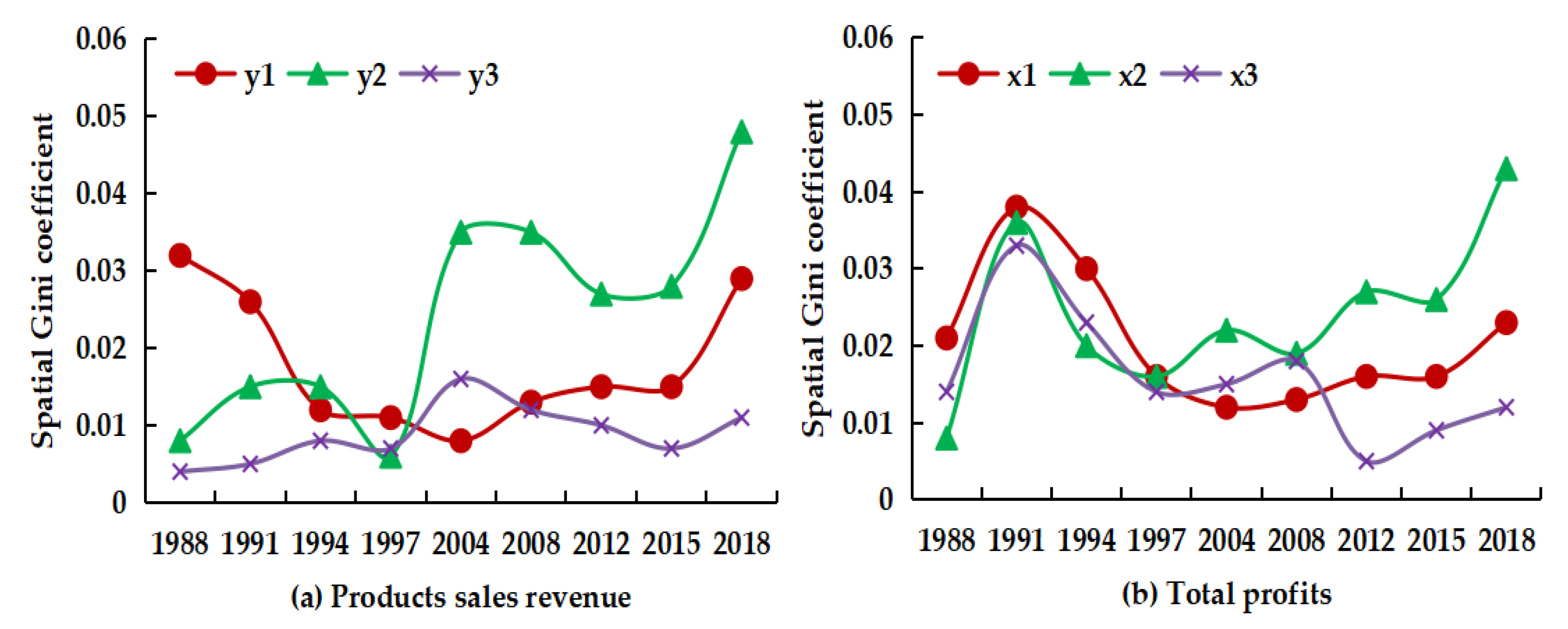
The conclusions are as follows. Firstly, the spatial agglomeration degree of China’s forest products manufacturing industry was not high between 1988 and 2018. The spatial Gini coefficients of the wood processing industry, furniture manufacturing industry and paper industry did not exceed 0.024. Secondly, the core regions of the spatial agglomeration of China’s forest products manufacturing industry are Jiangsu, Zhejiang, Jiangxi, Shandong, Anhui, Henan, Hunan, Hubei, Guangxi, Fujian and Guangdong, 11 provinces that are mainly located in the southeast coastal areas of China. Thirdly, the spatial agglomeration direction of the forest products manufacturing industry has a “two-way agglomeration” trend of “northeast to southwest” and “northwest to southeast”, and the barycenter of industrial distribution in the sample period shows a trend of moving south. In addition, the forest products manufacturing industry is mainly characterized by a high–high and low–low spatial agglomeration pattern. The high–high-type agglomeration provinces are mainly distributed in the eastern coastal area, and the number is relatively small. Finally, the spatial agglomeration location of the forest products manufacturing industry may be simultaneously affected by multiple factors, such as forest protection policies, raw material sources, international trade and the degree of marketization.

Based on the above research conclusions, the policy implications are as follows. Firstly, the scale economic effect of China’s forest products manufacturing industry has not been fully realized. Chinese government departments should establish a modern national forestry industry demonstration park and a timber-processing trade zone in Jiangsu, Zhejiang, Jiangxi, Shandong, Anhui, Henan, Hunan, Hubei, Guangxi, Fujian, Guangdong and other provinces, reduce taxes and fees for small and medium-sized forest products manufacturing enterprises and incentivize enterprises from other regions to continue congregating in southeast coastal areas. Large-scale forest products manufacturing enterprises can also continue to expand their production scale through mergers, reorganization and acquisition [65] to form 3–5 world-class large-scale furniture, wood-based panels, wood pulp and paper enterprises.

Secondly, the Chinese government should strengthen trade ties with overseas timber-exporting countries, such as Russia, New Zealand, Canada, the United States and Australia, and also develop high-quality artificial forests to broaden timber supply channels [65]. At present, the quality of artificial forests in China is poor, which is reflected not only in the scarcity of large-diameter timber and precious tree species, such as Juglans mandshurica, Fraxinus mandshurica, Pinus koraiensis and Phoebe bourneii, but also in the single structure of artificial forest species [2,74]. In the future, government departments should combine the development of artificial forests with the processing trade of forest products and scientifically plan and manage artificial forests to meet the development needs of forest products manufacturing [65].

Thirdly, the southeastern coastal provinces should optimize the regional industrial layout, and encourage three wood-based industries to form a co-agglomeration in Fujian, Shandong, Jiangsu, Zhejiang and Guangdong, and other provinces. Chinese local governments should take the initiative to guide the wood processing, the furniture manufacturing and the paper enterprises to avoid going alone individually, and use the industrial chain as a link to strengthen business cooperation between them. At the same time, export and non-export enterprises should cooperate. China Timber and Wood Products Distribution Association, China National Furniture Association and China Paper Association can strengthen guidance and promote the sharing of market information and coordination of production activities within the association. The spatial agglomeration of export-oriented enterprises is conducive to saving trade-related production costs and information costs [47,48]. The co-agglomeration of export-oriented and non-export-oriented enterprises is more convenient for exchanging international and local market information, and it is also conducive to the circumvention of horizontal competition to a large extent, allowing enterprises to adjust to the target market quickly.

References

1. Li, L.; Li, F.; Tao, C.; Cheng, B. The impact of spatial agglomeration on export of forest products manufacturing in China: Evidence from enterprises’ data. J. Sustain. For. 2019, 38, 743–754. [Google Scholar] [CrossRef]
2. Ke, S.; Qiao, D.; Zhang, X.; Feng, Q. Changes of China’s forestry and forest products industry over the past 40 years and challenges lying ahead. For. Policy Econ. 2021, 123, 102352. [Google Scholar] [CrossRef]
3. 2018 China Forestry and Grassland Development Statistical Bulletin. Available online: http://www.forestry.gov.cn/main/62/index.html (accessed on 8 March 2021).
4. Jiang, Y.; Chen, S. Trade Competitiveness of China’s Forest Products Manufacturing Analysis Based on Domestic Value Added. For. Econ. 2016, 38, 54–61. (In Chinese) [Google Scholar]
5. Qian, X. Current Status and Development Trends of China’s Forest Products Industry. Wood Ind. 2009, 23, 1–4. (In Chinese) [Google Scholar]
6. Quah, D. Spatial Agglomeration Dynamics. Am. Econ. Rev. 2002, 92, 247–252. [Google Scholar] [CrossRef]
7. Mori, T.; Smith, T.E. On the spatial scale of industrial agglomerations. J. Urban Econ. 2015, 89, 1–20. [Google Scholar] [CrossRef] [Green Version]
8. Cainelli, G.; Ganau, R.; Giunta, A. Spatial agglomeration, Global Value Chains, and productivity. Micro-evidence from Italy and Spain. Econ. Lett. 2018, 169, 43–46. [Google Scholar] [CrossRef]
9. Athukorala, P.; Narayanan, S. Economic corridors and regional development: The Malaysian experience. World Dev. 2018, 106, 1–14. [Google Scholar] [CrossRef] [Green Version]
10. Labuschagne, C.; Brent, A.C.; van Erck, R.P.G. Assessing the sustainability performances of industries. J. Clean Prod. 2005, 13, 373–385. [Google Scholar] [CrossRef] [Green Version]
11. Gao, L.; Li, F.; Zhang, J.; Wang, X.; Hao, Y.; Li, C.; Tian, Y.; Yang, C.; Song, W.; Wang, T. Study on the Impact of Industrial Agglomeration on Ecological Sustainable Development in Southwest China. Sustainability 2021, 13, 1301. [Google Scholar] [CrossRef]
12. Grazi, F.; Waisman, H.; Bergh, J.C.J.M. Agglomeration economies and spatial sustainability. IOP Conf. Ser. Earth Environ. Sci. 2009, 6, 432004. [Google Scholar] [CrossRef]
13. Daian, G.; Ozarska, B. Wood waste management practices and strategies to increase sustainability standards in the Australian wooden furniture manufacturing sector. J. Clean Prod. 2009, 17, 1594–1602. [Google Scholar] [CrossRef]
14. Krugman, P. Increasing Returns and Economic Geography. J. Polit. Econ. 1991, 99, 483–499. [Google Scholar] [CrossRef]
15. Tao, C.; Zhang, J.; Cheng, B.; Liu, Y. An Assessment of the Impact of Spatial Agglomeration on the Quality of China’s Wood Processing Industry Products. Sustainability 2019, 11, 3961. [Google Scholar] [CrossRef] [Green Version]
16. Porter, M.E. Clusters and the new economics of competition. Harv. Bus. Rev. 1998, 76, 77–90. [Google Scholar] [PubMed]
17. Krugman, P. Geography and Trade; Leuven University Press: Leuven, Belgium, 1991. [Google Scholar]
18. Marshall, A. Principles of Economics; Macmillan: London, UK, 1895. [Google Scholar]
19. Hotelling, H. Stability in Competition. Econ. J. 1929, 39, 41–57. [Google Scholar] [CrossRef]
20. Hoover, E.M. Location Theory and the Shoe Leather Industries; Harvard University Press: Cambridge, MA, USA, 1936. [Google Scholar]
21. Perroux, F. The Theory of Monopolistic Competition: A General Theory of Economic Activity. Indian Econ. Rev. 1955, 2, 134–143. [Google Scholar]
22. Hirschman, A.O. The Strategy of Economic Development; Yale University Press: New Haven, CT, USA, 1958; Volume 10. [Google Scholar]
23. Krugman, P. First Nature, Second Nature and Metropolitan Location. J. Reg. Sci. 1993, 33, 129–144. [Google Scholar] [CrossRef] [Green Version]
24. Fujita, M.; Krugman, P. The new economic geography: Past, present and the future. Pap. Reg. Sci. 2003, 83, 139–164. [Google Scholar] [CrossRef]
25. Alkay, E.; Hewings, G.J.D. The determinants of agglomeration for the manufacturing sector in the Istanbul metropolitan area. Ann. Reg. Sci. 2012, 48, 225–245. [Google Scholar] [CrossRef]
26. LI, L.M.Y. Spatial-temporal Pattern Evolution of Manufacturing Geographical Agglomeration and Influencing Factors of Old Industrial Base: A Case of Jilin Province, China. Chin. Geogr. Sci. 2015, 25, 486–497. [Google Scholar] [CrossRef]
27. Li, C.; Wu, K.; Gao, X. Manufacturing industry agglomeration and spatial clustering: Evidence from Hebei Province, China. Environ. Dev. Sustain. 2020, 22, 2941–2965. [Google Scholar] [CrossRef]
28. Luo, L.; Zheng, Z.; Luo, J.; Jia, Y.; Zhang, Q.; Wu, C.; Zhang, Y.; Sun, J. Spatial Agglomeration of Manufacturing in the Wuhan Metropolitan Area: An Analysis of Sectoral Patterns and Determinants. Sustainability 2020, 12, 8005. [Google Scholar] [CrossRef]
29. Jordaan, J.A.; Roiguez-Oreggia, E. Regional growth in Mexico under trade liberalization: How important are agglomeration and FDI? Ann. Reg. Sci. 2012, 48, 179–202. [Google Scholar] [CrossRef] [Green Version]
30. Brunello, G.; Langella, M. Local agglomeration, entrepreneurship and the 2008 recession: Evidence from Italian industrial districts. Reg. Sci. Urban Econ. 2016, 58, 104–114. [Google Scholar] [CrossRef] [Green Version]
31. Cheng, Z. The spatial correlation and interaction between manufacturing agglomeration and environmental pollution. Ecol. Indic. 2016, 61, 1024–1032. [Google Scholar] [CrossRef]
32. Fang, J.; Tang, X.; Xie, R.; Han, F. The effect of manufacturing agglomerations on smog pollution. Struct. Chang. Econ. Dyn. 2020, 54, 92–101. [Google Scholar] [CrossRef]
33. Zhao, H.; Cao, X.; Ma, T. A spatial econometric empirical research on the impact of industrial agglomeration on haze pollution in China. Air Qual. Atmos. Health 2020, 13, 1305–1312. [Google Scholar] [CrossRef]
34. Fukao, K.; Kravtsova, V.; Nakajima, K. How important is geographical agglomeration to factory efficiency in Japan’s manufacturing sector? Ann. Reg. Sci. 2014, 52, 659–696. [Google Scholar] [CrossRef] [Green Version]
35. Azari, M.; Kim, H.; Kim, J.Y.; Ryu, D. The effect of agglomeration on the productivity of urban manufacturing sectors in a leading emerging economy. Econ. Syst. 2016, 40, 422–432. [Google Scholar] [CrossRef]
36. Yuan, H.; Feng, Y.; Lee, C.; Cen, Y. How does manufacturing agglomeration affect green economic efficiency? Energy Econ. 2020, 92, 104944. [Google Scholar] [CrossRef]
37. Antonietti, R.; Antonietti, R.; Cainelli, G.; Cainelli, G. The role of spatial agglomeration in a structural model of innovation, productivity and export: A firm-level analysis. Ann. Reg. Sci. 2011, 46, 577–600. [Google Scholar] [CrossRef]
38. Liang, J.; Goetz, S.J. Technology intensity and agglomeration economies. Res. Policy 2018, 47, 1990–1995. [Google Scholar] [CrossRef]
39. Henderson, J.V. Marshall’s scale economies. J. Urban Econ. 2003, 53, 1–28. [Google Scholar] [CrossRef]
40. Brülhart, M.; Mathys, N.A. Sectoral agglomeration economies in a panel of European regions. Reg. Sci. Urban Econ. 2008, 38, 348–362. [Google Scholar] [CrossRef] [Green Version]
41. Stojčić, N.; Anić, I.; Aralica, Z. Do firms in clusters perform better? Lessons from wood-processing industries in new EU member states. For. Policy Econ. 2019, 109, 102043. [Google Scholar] [CrossRef]
42. Hu, S.; Song, W.; Li, C.; Zhang, C.H. The Evolution of Industrial Agglomerations and Specialization in the Yangtze River Delta from 1990–2018: An Analysis Based on Firm-Level Big Data. Sustainability 2019, 11, 5811. [Google Scholar] [CrossRef] [Green Version]
43. Lu, J.; Tao, Z. Trends and determinants of China’s industrial agglomeration. J. Urban Econ. 2009, 65, 167–180. [Google Scholar] [CrossRef] [Green Version]
44. Ellison, G.; Glaeser, E.L. Geographic Concentration in U.S. Manufacturing Industries: A Dartboard Approach. J. Polit. Econ. 1997, 105, 889–927. [Google Scholar] [CrossRef] [Green Version]
45. Arbia, G.; Espa, G.; Giuliani, D.; Dickson, M.M. Spatio-temporal clustering in the pharmaceutical and medical device manufacturing industry: A geographical micro-level analysis. Reg. Sci. Urban Econ. 2014, 49, 298–304. [Google Scholar] [CrossRef]
46. Behrens, K.; Bougna, T. An anatomy of the geographical concentration of Canadian manufacturing industries. Reg. Sci. Urban Econ. 2015, 51, 47–69. [Google Scholar] [CrossRef] [Green Version]
47. He, C.; Wang, J. Geographical agglomeration and co-agglomeration of foreign and domestic enterprises: A case study of Chinese manufacturing industries. Post-Communist Econ. 2010, 22, 323–343. [Google Scholar] [CrossRef]
48. He, C.; Guo, Q.; Ye, X. Geographical agglomeration and co-agglomeration of exporters and nonexplorers in China. GeoJournal 2016, 81, 947–964. [Google Scholar] [CrossRef]
49. Tao, C.; Li, L.; Cheng, B. An Empirical Study on the Spatial Agglomeration Level of China’s Wood-Processing Industry. J. Beijing For. Univ. Soc. Sci. 2017, 16, 61–68. (In Chinese) [Google Scholar]
50. Li, L.; Tao, C.; Cheng, B. Empirical Study on Spatial Agglomeration of Paper-making Industry in China. For. Econ. 2017, 39, 40–44. (In Chinese) [Google Scholar]
51. Xia, Y.; Shen, W. Agglomeration Level Measurement, Evolution Trend and Industrial Economic Growth of China’s Forest Products Industry: An Empirical Study Based on 2003–2016 Data. World For. Res. 2018, 31, 42–46. (In Chinese) [Google Scholar]
52. Yang, C.; Song, W.; Cheng, B. Study on Industrial Transfer and Agglomeration: Is Wood-processing Industry Agglomeration Excessive? For. Econ. 2018, 40, 16–21. (In Chinese) [Google Scholar]
53. Xia, Y.; Shen, W. Agglomeration, coagglomeration and labor productivity effects of wood processing industry. J. Nanjing For. Univ. Nat. Sci. Ed. 2019, 43, 131–136. (In Chinese) [Google Scholar]
54. Zeng, J.; Nie, Y. Panel Data Identification of Convergent and Divergent Power in Regional Furniture Industry Cluster: Empirical Analysis on Second Natural Factor. World For. Res. 2012, 25, 51–56. (In Chinese) [Google Scholar]
55. Aiginger, K.; Rossi-Hansberg, E. Specialization and concentration: A note on theory and evidence. Empirica 2006, 33, 255–266. [Google Scholar] [CrossRef]
56. Lefever, D.W. Measuring Geographic Concentration by Means of the Standard Deviational Ellipse. Am. J. Sociol. 1926, 32, 88–94. [Google Scholar] [CrossRef]
57. Yang, Z.; Xiu, Q.; Chen, D. Historical changes in the port and shipping industry in Hong Kong and the underlying policies. Transp. Policy 2019, 82, 138–147. [Google Scholar] [CrossRef]
58. Du, Q.; Zhou, J.; Pan, T.; Sun, Q.; Wu, M. Relationship of carbon emissions and economic growth in China’s construction industry. J. Clean Prod. 2019, 220, 99–109. [Google Scholar] [CrossRef]
59. Wachowicz, M.; Liu, T. Finding spatial outliers in collective mobility patterns coupled with social ties. Int. J. Geogr. Inf. Sci. 2016, 30, 1806–1831. [Google Scholar] [CrossRef]
60. Xu, F.; Li, H.; Bao, H. Performance comparisons of land institution and land regulation systems on water area decrease. Habitat Int. 2018, 77, 12–20. [Google Scholar] [CrossRef]
61. Richter, A.; Ng, K.T.W.; Karimi, N.; Chang, W. Developing a novel proximity analysis approach for assessment of waste management cost efficiency in low population density regions. Sustain. Cities Soc. 2021, 65, 102583. [Google Scholar] [CrossRef]
62. Ye, X.; Wu, L. Analyzing the dynamics of homicide patterns in Chicago: ESDA and spatial panel approaches. Appl. Geogr. 2011, 31, 800–807. [Google Scholar] [CrossRef]
63. Dou, Y.; Luo, X.; Dong, L.; Wu, C.; Liang, H.; Ren, J. An empirical study on transit-oriented low-carbon urban land use planning: Exploratory Spatial Data Analysis (ESDA) on Shanghai, China. Habitat Int. 2016, 53, 379–389. [Google Scholar] [CrossRef]
64. Lin, B.; Du, R.; Dong, Z.; Jin, S.; Liu, W. The impact of foreign direct investment on the productivity of the Chinese forest products industry. For. Policy Econ. 2020, 111, 102035. [Google Scholar] [CrossRef]
65. Su, H.; Hou, F.; Yang, Y.; Han, Z.; Liu, C. An assessment of the international competitiveness of China’s forest products industry. For. Policy Econ. 2020, 119, 102256. [Google Scholar] [CrossRef]
66. Liu, H.; Wang, Y.; Lei, M. Spatial agglomeration of strategic emerging industries in China. J. Quant. Tech. Econ. 2019, 36, 99–116. (In Chinese) [Google Scholar]
67. Peng, J.; Chen, S.; Lü, H.; Liu, Y.; Wu, J. Spatiotemporal patterns of remotely sensed PM2.5 concentration in China from 1999 to 2011. Remote Sens. Environ. 2016, 174, 109–121. [Google Scholar] [CrossRef]
68. Zhao, L.; Zhao, Z. Spatial Agglomeration of the Manufacturing Industry in China. J. Quant. Tech. Econ. 2014, 31, 110–121. (In Chinese) [Google Scholar]
69. Anselin, L. Local Indicators of Spatial Association—LISA. Geogr. Anal. 1995, 27, 93–115. [Google Scholar] [CrossRef]
70. Meng, D.; Wei, G.; Sun, P.; Li, H. Analyzing the Characteristics and Causes of Location Spatial Agglomeration of Listed Companies: An Empirical Study of China’s Yangtze River Economic Belt. Complexity 2020, 2020, 8859706. [Google Scholar] [CrossRef]
71. Démurger, S.; Yuanzhao, H.; Weiyong, Y. Forest Management Policies and Resource Balance in China: An Assessment of the Current Situation. J. Environ. Dev. 2009, 18, 17–41. [Google Scholar] [CrossRef] [Green Version]
72. Delang, C.O.; Wang, W. Chinese Forest Policy Reforms after 1998: The Case of the Natural Forest Protection Program and the Slope Land Conversion Program. Int. For. Rev. 2013, 15, 290–304. [Google Scholar] [CrossRef]
73. Yu, D.; Zhou, L.; Zhou, W.; Ding, H.; Wang, Q.; Wang, Y.; Wu, X.; Dai, L.; He, H.S.; Shifley, S.R.; et al. Forest Management in Northeast China: History, Problems, and Challenges. Environ. Manag. 2011, 48, 1122–1135. [Google Scholar] [CrossRef]
74. Hou, J.; Yin, R.; Wu, W. Intensifying Forest Management in China: What does it mean, why, and how? For. Policy Econ. 2019, 98, 82–89. [Google Scholar] [CrossRef]
75. Dai, L.; Li, S.; Zhou, W.; Qi, L.; Zhou, L.; Wei, Y.; Li, J.; Shao, G.; Yu, D. Opportunities and challenges for the protection and ecological functions promotion of natural forests in China. For. Ecol. Manag. 2018, 410, 187–192. [Google Scholar] [CrossRef]
Figure 1. Spatial distribution of forest products manufacturing industry (product sales revenue).
Forests 12 01006 g001aForests 12 01006 g001b
Figure 2. Spatial distribution of forest products manufacturing industry (total profits).
Forests 12 01006 g002
Figure 3. Development of China’s forest products manufacturing industry by province.
Forests 12 01006 g003
Figure 4. Spatial Gini coefficient of China’s forest products manufacturing industry.
Forests 12 01006 g004
Figure 5. Standard deviation ellipse (SDE) of China’s forest products manufacturing industry.
Forests 12 01006 g005
Figure 6. Moran scatter plot of China’s forest products manufacturing industry (product sales revenue).
Forests 12 01006 g006
Figure 7. Moran scatter plot of China’s forest products manufacturing industry (total profits).
Forests 12 01006 g007