
Spatially Explicit Kirtland’s Warbler Habitat Management Scheduling in Michigan’s Upper Peninsula †


1
USDA Forest Service Northern Region, 26 Fort Missoula Road, Missoula, MT 59804, USA
2
Department of Forest Resources and NC Research and Outreach Center, University of Minnesota, Grand Rapids, MN 55744, USA
*
Author to whom correspondence should be addressed.
†
This work was part of a dissertation of the corresponding author Eric Henderson, PhD program at the University of Minnesota, St. Paul, MN, USA.
Forests 2021, 12(8), 1065; https://0-doi-org.brum.beds.ac.uk/10.3390/f12081065
Submission received: 30 April 2021
/
Revised: 10 June 2021
/
Accepted: 4 August 2021
/
Published: 10 August 2021
(This article belongs to the Special Issue Forest Management and Economics: Integrating Objectives Using Harvest Scheduling and Operations Research)
Abstract
:A spatially explicit management strategy is presented for Kirtland’s Warbler (Setophaga kirtlandii) habitat on the Hiawatha National Forest in Michigan’s Upper Peninsula. The Hiawatha National Forest has a goal of continuously providing large patches of dense young jack pine for Kirtland’s warbler breeding habitat. The problem is challenging as patches of suitable habitat are relatively short lived, forcing large shifts in the location of large patches in the future. In this study, alternative management strategies for providing habitat are described, explicitly mapped, and compared on a 70,600 ha landscape in the context of implementing many desired conditions of the forest’s land management plan. Strategies are developed by using two interacting scheduling models. Comparisons address overall habitat levels, habitat spatial arrangement through time, and financial trade-offs. The financial cost of managing habitat is high and there are further financial trade-offs associated with aggregating habitat into large patches. Furthermore, the marginal cost of habitat increases as more habitat is added to the management system. Managers may use information about the added costs of spatially explicit habitat management to help evaluate the added benefits to the species. It is often expensive to establish wildlife habitat and desirable ecological conditions, but results show that there are potential benefits from using detailed computer-aided management scheduling tools to support the decision-making process.
1. Introduction
1.1. Kirtland’s Warbler Habitat Management
The Kirtland’s warbler (Setophaga kirtlandii) breeding range is one of the smallest regions of any mainland bird in the continental United States [1]. Since monitoring began in 1951, over 98% of the population has been detected in jack pine (Pinus banksiana) stands in Lower Michigan, and since 2000, 86% of the population has been detected in just five counties [2]. The Kirtland’s warbler was listed as endangered in 1973 on the initial list of the Federal Endangered Species Act (16 U.S.C. 1531 et seq) until it was delisted in 2019. Active habitat management has proven to be an effective recovery strategy. A Recovery Plan drafted in 1976 recommended creation of 15,379 ha of warbler breeding habitat in northern Lower Michigan, and has resulted in the warbler’s recovery from a low of 167 singing males in 1974 to 2365 singing males recorded in 2015 [3,4]. Kirtland’s warbler is a conservation reliant species, as continued active management is necessary to maintain a stable population [5]. Brown et al. [6] simulated active management into the future, consisting of both habitat management and parasitic control. They projected long-term persistence and stability of the species so long as active management continued on the landscape. The delisting from the Endangered Species Act, however, requires a monitoring plan which includes a tabulation of the amount and proximity of available habitat and population levels for at least five years [7]. Additionally, the Kirtland’s warbler conservation plan specifies future contributions to breeding habitat from various land management agencies to support persistent population levels [4].
Kirtland’s warbler population increases have resulted in the expansion of the its breeding range. Before 1995, the Kirtland’s warbler had been sighted outside of the Lower Peninsula of Michigan but breeding activity had not been detected. Since 1995, breeding activity has been detected with consistency in Michigan’s Upper Peninsula, and in 2007 the first nests were recorded in Wisconsin and Canada [8,9,10]. Thus, the warbler’s recovery appears to have resulted in population levels that have saturated the Lower Peninsula breeding habitat and facilitated colonization in geographic areas outside the Lower Peninsula. This also indicates that dispersal of the species both within and between breeding seasons does not seem to be inhibited by distance or large water bodies [8]. There may be a temporal lag, however, in habitat occupation when population levels are low relative to the amount of available habitat and the distance to the nearest occupied patch is high [11]. To visualize the extent of colonization, the Kirtland’s Warbler Breeding Range Conservation Plan shows the extent and magnitude of the singing male population from 2005 to 2012 detected in Wisconsin and Michigan [4].
Expansion into new geographic ranges presents both an opportunity and a challenge to forest managers who are concerned about the persistence or expansion of the species but are not poised to execute management strategies to create and maintain suitable warbler breeding habitat. Establishing habitat in a landscape can be challenging due to the biological conditions it requires. Suitable habitat characteristics have been described by Probst [12] and Kashian, Barnes and Walker [13]. The desired habitat occurs in young jack pine (Pinus banksiana), has a short tenure (10–20 years depending on site characteristics), relatively high stocking densities in patchy distributions, and a generally cited minimum patch size of 32 ha (e.g., Probst and Weinrich [14]). Small patches, however, are not all that efficient in maintaining a breeding population. Probst and Weinrich [14] cite that 77% of the singing males were found in patches larger than 200 ha from 1979 to 1989. Donner, Ribic, and Probst [15] found that larger, non-isolated patches were associated with earlier colonization and later abandonment. Larger patches tended to have a longer duration of occupancy, and patches close to currently occupied habitat were colonized earlier. Historically, a 80.9 ha patch size standard has been used to establish Kirtland’s warbler breeding areas [12]. Management guidance has more recently been adopted by public agencies in Michigan and Wisconsin that are capable of maintaining warbler habitat [11]. This guidance includes recommendations to design habitat treatment blocks 120 ha or greater in size and at least 400 m wide.
A complicating factor in designing habitat in a newly colonized geographic area arises when there is existing management plan guidance for the landowner, as is the case for National Forests. While areas in Michigan’s Lower Peninsula are dedicated to the production and maintenance of Kirtland’s warbler habitat, management in newly colonized areas typically must consider additional management objectives for other ecological conditions such as a mix of forest cover types [13]. Flexibility in where and when to create habitat within the larger context of forest management planning priorities adds substantial complexity to the problem, i.e., analyzing forest cover type conversion options, spatial arrangement of those options, associated habitat through time, and impacts on other forest cover type objectives.
Another factor complicating the design of habitat is the financial investment required to create suitable habitat. Financial investments can be substantial due to increased stocking densities that require planting more seedlings. Financial costs can also be indirect; for instance, compromising the optimal timber rotation age or converting a more valuable tree species to the less valuable jack pine. While timber revenues can help offset the costs of implementation activities, they are prone to fluctuating market conditions [4]. Consequently, limited resources have historically impeded the full implementation of habitat creation objectives [16]. Earlier studies have emphasized minimizing the costs of management necessary to increase the likelihood of species’ persistence and minimum population sizes [17,18]. Since population increases have resulted in the species being delisted, habitat management appears effective, and arguably helps justify past investments [2,4,19]. Yet, as the species is conservation-reliant, additional large and reoccurring investments are needed to maintain the relatively short-lived suitable habitat [5]. With fire suppression limiting natural forest fire activity in the Lake States [4], establishing dense jack pine stands with mechanical means can be expensive.
1.2. Operations Research-Based Methods to Address Spatial and Temporal Complexities
Operations research based models can be used to analyze forest management problems with spatial and temporal complexity such as Kirtland’s warbler habitat planning. Historically, exact mathematical formulations were often too large to solve with standard mathematical programming. In response, solutions relied on metaheuristics such as genetic algorithms, simulated annealing, and tabu search [20]. For forestry applications, Kangas et al. [20] provide a review of heuristic optimization including metaheuristics that have been linked with optimization models.
Simplifying the temporal or spatial resolution of a planning problem is another approach to feasibly solving complex forestry problems with exact methods. Andersson and Eriksson [21] evaluated temporal simplification and found that five-year planning periods were generally adequate for representing financial returns from timber production. Yet, temporal and spatial simplification in planning problems does not always result in desirable outcomes. Rau et al. [22] reviewed 295 studies on ecosystem services and found that only 2% of those studies considered changes over time. They emphasized that future studies should: (1) more explicitly consider fine-grain temporal patterns, (2) analyze trade-offs and synergies between services over time, and (3) integrate changes in supply and demand through time.
Dynamic programming (DP) is a problem structure from operations research that has been useful in analyzing temporally and spatially complex forestry problems. DP decomposes large problems into a series of smaller, linked problems that can result in a problem of reasonable size [23]. A notable challenge with forestry-based DP formulations is they grow rapidly in size with moderate increases in the number of management options recognized for each stand, also known as the “curse of dimensionality” [23]. To address DP size concerns, Hoganson and Borges [24] and Borges, Hoganson, and Rose [25] developed a heuristic model that solved large DP problems with a series of overlapping subproblems, or “moving windows”. They called this heuristic model DPSpace. The first DPSpace applications were to address forestry problems with adjacency constraints. Later, Hoganson et al. [26] applied DPSpace to solve a core area problem to aggregate stands and minimize influences from stand edges. The model was used operationally as part of the USDA Forest Service planning process for the two National Forests in Minnesota [27]. Wei and Hoganson [28] investigated DPSpace parameter settings with the goal of quickly solving problems with minimal effects on quality. Their main tests specific to window design showed that while smaller window sizes resulted in shorter solution times, they also yielded inferior solution values. Some of these challenges were addressed by Henderson and Hoganson [29] who developed a heuristic method to quickly identify high quality solutions by comparing and learning from solutions to multiple DPSpace formulations. Later stages of this process allow analyses to focus on areas of the forest where optimal solutions are more difficult to identify, such as where multiple proximal stands have similar management opportunities that result in a large number of spatial permutations.
Another challenge with dynamic programming formulations is they do not directly consider forest-wide resource constraints such as even-flow of timber, harvest limits, or minimum levels of wildlife habitat. To accommodate this limitation, marginal values (also known as shadow prices or dual prices) can be estimated and included in the value of each management option in the DP formulation. Marginal values are the foregone financial revenues from choosing a management schedule to meet a vegetation constraint instead of the timber-optimal schedule. One such tool to estimate these values is the DualPlan model, first described by Hoganson and Rose [30]. The DualPlan model iteratively adjusts marginal value estimates based on whether the current solution is in either the infeasible or suboptimal regions relative to forest-wide constraints.
These two models (DualPlan and DPSpace) were linked and utilized in forest planning in Minnesota to address core area of mature forest [31,32,33]. Wei and Hoganson [28] found that near-optimal solutions could be found for situations in Minnesota involving tens of thousands of stands. For these studies core area was scheduled by explicitly testing different valuations of core area of older forest, but did not explicitly constrain the desired level of core area. The time dimension of the Minnesota studies was simplified to 10-year planning periods, which may not be ideally situated for Kirtland’s warbler management planning based on their use of habitat.
1.3. Study Application Area
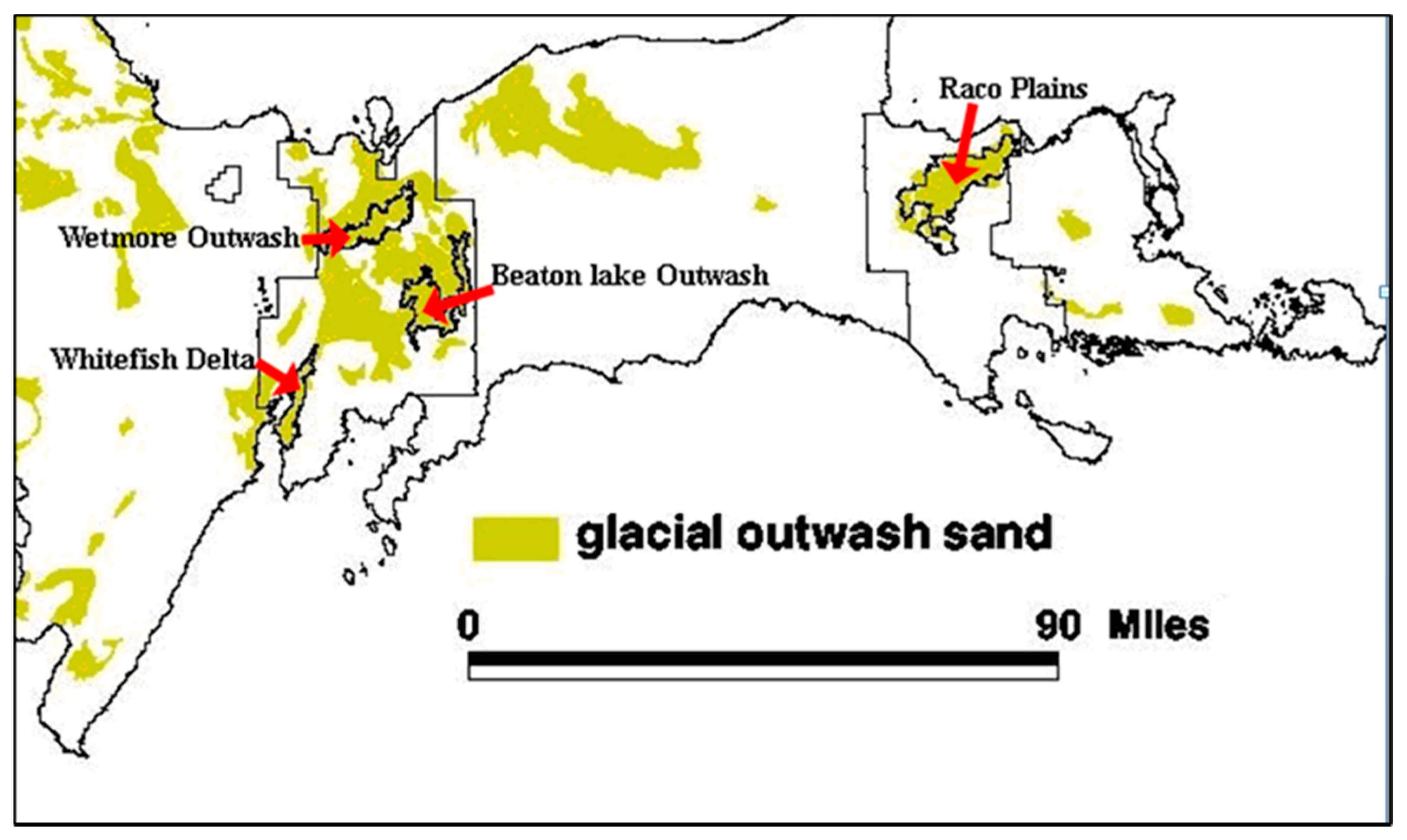
The Hiawatha National Forest in Michigan’s Upper Peninsula is a geographic area colonized by the Kirtland’s warbler since recovery efforts began (Figure 1). The forest is comprised of approximately 362,200 ha in two distinct ownership units of comparable size. The 2006 Hiawatha National Forest Plan [34] has made a commitment to manage for Kirtland’s warbler breeding habitat within these boundaries. Ecological conditions for suitable breeding habitat can be found on four distinct glacial outwash plains of the Hiawatha National Forest (Figure 1). These four outwash plains are delineated into approximately 12,300 management units (stands) representing 70,600 ha. Of this total area, the Forest has agreed to manage 13,600 ha (20%) in a Kirtland’s warbler habitat system consisting of jack pine stands between 0 and 50 years of age, of which 2711 ha are targeted to be suitable breeding habitat (age 6–16 years) at any given time [35]. The 6–16 age range is based on better site conditions of the forest, and thus shorter suitable conditions, than studies in Lower Michigan where the maximum age of occupancy was 23 [14,35]. The desire to maintain a consistent amount of breeding habitat through time is consistent with the direction of the original recovery plan and the existing conservation plan [3,11]. The stem densities of these habitat blocks are to correspond with the latest science provided by the U.S. Fish and Wildlife Service. The plan specifies that patches of habitat can be generated in blocks of up to 445 ha with a single management activity. The specific stands managed as suitable breeding habitat and the spatial arrangement or patch shape of the habitat, however, have not been explicitly identified. For each point in time, the Hiawatha National Forest has discretion in where it places the 2711 ha of breeding habitat within the 70,600 ha available, and therefore can design a financially efficient management system that is effective for producing both Kirtland’s warbler habitat and other desired forest conditions.
The Hiawatha National Forest Plan [35] identifies an array of desired future conditions that describe diverse forest cover types and size classes in addition to warbler habitat, including red pine (Pinus resinosa), aspen (Populus tremuloides), mixed pine (Pinus spp.) and oak (Quercus spp.) cover types, and maintained forest openings. Management direction does not identify Kirtland’s warbler habitat as more (or less) important than the other desired conditions, and therefore should not be prioritized above other desired conditions. The intent of this study is to provide forest managers with information about the spatial opportunities where habitat could be managed through time. Additionally, this study will explore the trade-offs and impacts on other desired conditions that may occur when meeting spatial goals for Kirtland’s warbler habitat.
1.4. Objectives
The objective of this study was to explore the opportunity and trade-offs associated with spatially explicit management schedules for Kirtland’s warbler breeding habitat through time. Specifically, the study sought to provide insight to the following questions:
- How well does the modeling system used in this study perform in identifying a spatially explicit management strategy for arranging breeding habitat?
- In the context of multiple forest objectives, what are the trade-offs associated with managing for large habitat patches compared to managing habitat without spatial consideration?
- What are the financial trade-offs between alternative spatial management intensities?
2. Materials and Methods
2.1. Operations Research-Based Scheduling Methods for Spatial Arrangement
Management schedules for the forest were developed by linking and expanding two planning models described above: DualPlan [30] and DPSpace [24,34]. DualPlan was used to estimate the marginal value of desired conditions (or constraints), and DPSpace used these values to schedule stands in a spatial context, in this instance to achieve the core area constraints for Kirtland’s warbler habitat. The forest-wide modeling process is an iterative one; that is, the DPSpace solution is used to evaluate how well all constraint levels are met, both spatial (core area levels) and non-spatial (other forest-wide desired conditions). If the solution does not meet constraint levels, DualPlan is called again to re-estimate marginal values, and the process continues until an acceptable solution is reached. Specifics of the DPSpace formulation used in this study are described in Henderson and Hoganson [29].
In this study, the desired level of Kirtland’s warbler habitat was defined as either the total amount of habitat area or the amount of habitat in core area. Total habitat is simply the sum of all hectares of habitat that meet the appropriate age and vegetation conditions, regardless of patch size or arrangement on the landscape. Core area was the habitat at least 37 m from the nearest edge [36]. Core area calculation was simplified by partitioning the landscape into 0.81 ha hexagons and using the centers of the surrounding six hexagons to define the 37 m buffer (Figure 2). We acknowledge that the buffer distance around the center cell is slightly irregular, but the simplification is consistent throughout the forest and is unlikely to bias results in any particular area. The stand boundaries and the associated buffers are approximations of spatial realities, much like raster squares and irregular polygons. Hexagons, however, have regular spatial relationships with all six adjacent hexagon cells, which is not the case for maps based on squares or irregular polygons [37]. The forest’s vector-based stand layer was intersected with a hexagon grid to assign a vegetation condition to each hexagon. To illustrate the difference between total habitat and core area habitat, consider stands 1, 3, and 4 in Figure 2, each represented as a single hexagon. If these three stands meet habitat requirements in period t, the resulting core area in period t would be the area inside the triangle, and the total amount of habitat would be the total area of the three stands.
2.2. Planning Horizon and Time Periods
The planning horizon in this study was 60 years, modeled as a series of 30 two-year time periods. Sixty years was chosen to examine a planning horizon longer than the recommended jack pine rotation length of 50 years, as well as to allow other cover types with longer rotations, such as red pine (Pinus resinosa), to convert to the Kirtland’s warbler habitat system where appropriate. Using short, two-year planning periods allows one to better refine timing options, thus recognizing more potential management coordination with neighboring stands over time. Finer temporal resolution helps refine the timing of when managers should create the habitat. With two-year planning periods, each regeneration activity produces habitat in five periods when it is aged 6–16 years old. The narrow temporal window for suitable habitat conditions paired with the concern that breeding is an annual event with even a single year of limited breeding habitat could have implications to the overall species population. Coarser time periods, such as 5 years, result in more ambiguity in important temporal detail. For instance, two adjacent stands regenerated in consecutive 5 year time periods could jointly produce habitat for either 9 years (stand 1 regenerates at the end of period 1 and stand 2 regenerates at the beginning of period 2), 1 year (stand 1 regenerates at beginning of period 1 and stand 2 regenerates at end of period 2) or any length of time in between.
2.3. Stand Management Options and Costs
A wide range of management timing choices and forest cover type conversion options were considered for most stands in the forest. The outwash plains ecosystem in the Upper Peninsula of Michigan where Kirtland’s warbler habitat is found has historically supported a mix of short- and long-lived species, open savannahs, and small inclusions of broad-leafed species [38]. The spatial arrangement of these different cover types and age classes is dynamic, and the current arrangement is a function of past management and disturbance.
The many management options available with two-year planning periods adds substantial complexity to the management situation. Not only do the potential harvest timings of an existing stand increase, but so do the timings and cover type options for future rotations and for neighboring stands. Most existing upland forest cover types were considered feasible for converting to Kirtland’s warbler habitat. For the 12,307 stands recognized in this study, there were a total of 1.08 million management options considered, an average of 88 per stand.
Each stand-level management option had an associated set of economic inputs and outputs that included costs, revenues, and timber volumes. These metrics were included to help examine trade-offs between alternative management strategies and were consistent with data used in the 2006 Forest Plan analysis. Costs included sale administration, planting, and site preparation activities. Generally, Kirtland’s warbler habitat regeneration is expensive due to increased site preparation and planting costs associated with higher stocking densities. The Hiawatha National Forest identified the average cost of regenerating jack pine at $968/ha and the cost of regenerating jack pine at Kirtland’s warbler stocking levels at $1879/ha.
2.4. Objective Function, Ending Inventory, and Forest-Wide Constraints
The management objective of the model was to maximize financial net present value (NPV) of the forest, calculated as net revenue discounted 4% annually. Spatial interactions between stands were considered beyond the sixty-year planning horizon by projecting conditions over an additional 120 years, using the same management interval scheduled during the first 60 years. Value was given to forest conditions and Kirtland’s warbler habitat beyond the end of the planning horizon to help ensure that ending inventory values do not assume atypical harvesting near the end of the planning horizon.
Forest-wide constraints were used to achieve the desired vegetation conditions described in the Hiawatha National Forest Management Plan [35] (Table 1). In the table, each constraint set is used for all 30 planning periods. Lower constraint types indicate a minimum desired level and upper constraint types indicate a maximum desired level. Additionally, several core area constraint levels were examined, described in the next section. Constraints on core are not enforced until period 6 (year 12) to allow the model sufficient time to adjust the current situation on the landscape. Specifically, at the start of the planning horizon there are 2544 ha of age 6–16 stands on the forest and an additional 2508 ha that will become suitable habitat within the next six years. The model has no control over creating more habitat until period 4—when jack pine regenerated in period 1 reaches the minimum stand age for suitable breeding habitat.
2.5. Model Benchmarks and Scenarios
Several benchmarks and scenarios were evaluated to provide information about model performance and trade-offs associated with Kirtland’s warbler habitat management. Benchmarks are incomplete model formulations intended to provide information about the impacts and costs of model constraints. Additionally, three scenarios varied the core area constraints to give managers insights into the trade-offs and costs of managing for breeding habitat at different forest-wide levels.
Benchmark 1 (B1: No habitat requirements) solves the forest management problem with all constraints except Kirtland’s warbler habitat constraints. This benchmark provides a basis for the financial value of the forest when only non-habitat desired conditions are considered and can subsequently be used to help estimate the total opportunity cost of habitat management.
Benchmark 2 (B2: Total Habitat) used a minimum constraint of 2711 ha of total Kirtland’s warbler habitat each period but did not constrain the amount of core area. All constraints from Table 1 were used. The benchmark provides a baseline for estimating the cost of arranging habitat spatially on the landscape. All hectares of jack pine stocked at appropriate habitat levels in the 6–16-year age range are considered as breeding habitat, regardless of patch size. The solution represents the expectations of the Hiawatha National forest at the time the plan was written.
Benchmark 3 (B3: Core area requirements only) uses a minimum constraint of 2226 ha of Kirtland’s warbler habitat core area as well as constraints to ensure a consistent timber harvest level through time (the final 2 constraint sets of Table 1). The other constraint sets in Table 1 are not used for Benchmark 3. This benchmark represents the maximum net financial value of the forest if core area habitat was the only management consideration other than financial value. This benchmark provides a basis for estimating the financial and spatial impacts of providing other cover type desired conditions on habitat patch and core area potential.
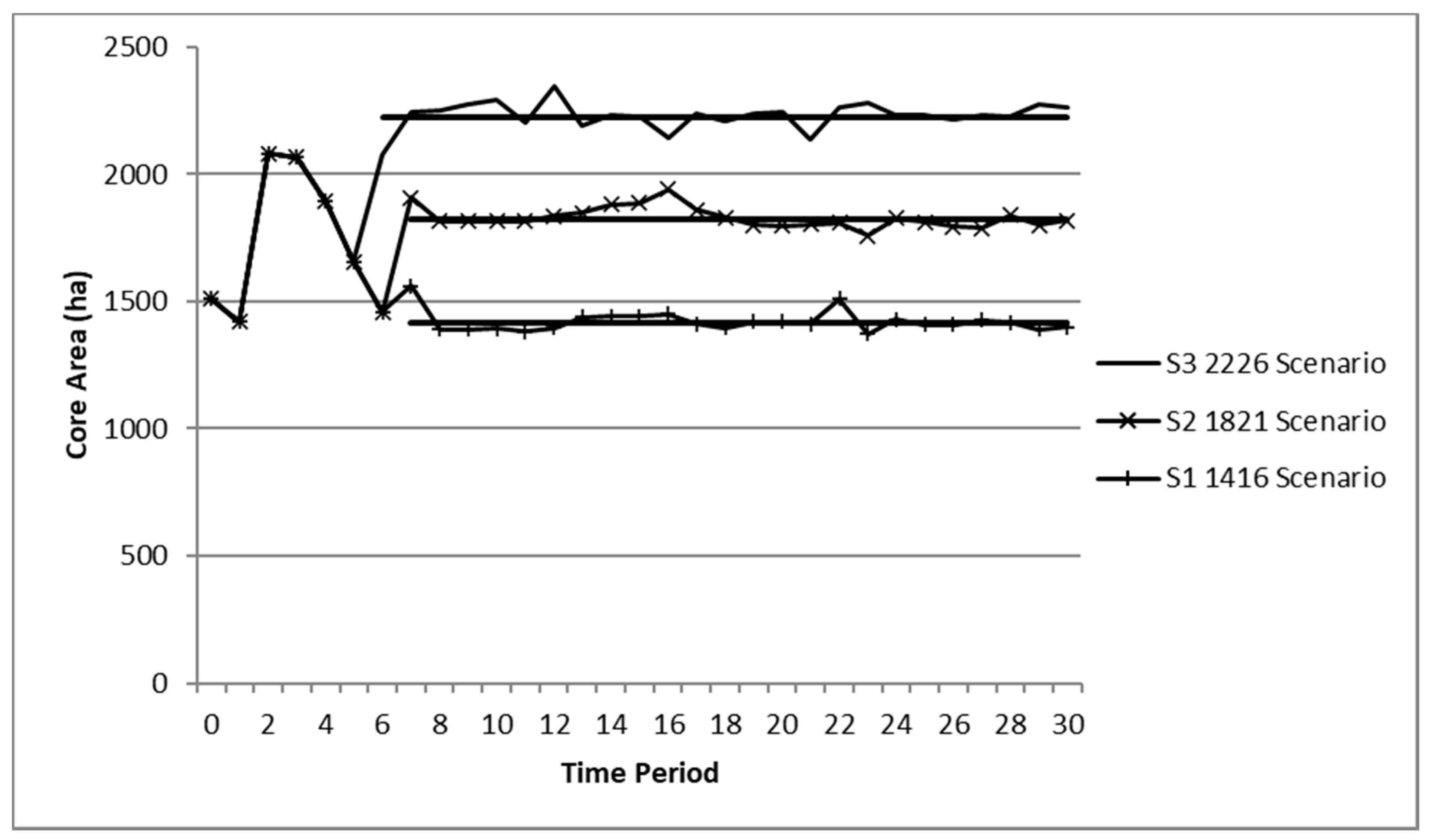
Three scenarios were evaluated with the forest-wide constraints described in Table 1. These scenarios varied the core area habitat constraints at 1416 ha (S1), 1821 ha (S2) and 2226 ha (S3). The total area of habitat (including area not satisfying core area requirements) was also calculated for these scenarios. These scenarios provide a basis for a trade-off analysis between managing for different amounts of Kirtland’s warbler habitat.
2.6. Identifying Acceptable Solutions
One phenomenon of the solution method presented here is the potential imprecision in satisfying the forest-wide constraints. There are usually small deviations in how well the accepted solution meets the desired constraint levels. Most often, these deviations can be attributed to the whole-stand scheduling nature of the problem, which may prevent fine-tuning to achieve exact constraint satisfaction. For the solutions presented here, each constraint was within 1% of the desired level cumulatively over all 30 planning periods.
One other challenge of a spatial problem is measuring the quality of the spatial arrangement in a solution. Ideally, habitat patches would be large and round to reduce the amount of buffering needed to produce the desired levels of core area. One common metric for measuring patch compactness is an edge to area ratio. A limitation with this metric is that its value changes with the relative size of the patch. For example, a small circle will have a high edge to area ratio relative to a larger circle [39]. Fortunately, compact patches are a natural result of valuing core area since a circular patch has the greatest amount of core area for any shape with the same area. Potential compactness of patches in practice is limited by the age and cover type heterogeneity of contiguous stands, as well as non-ownership, non-forested stands, or features such as roads, lakes, or lowland areas. Wei and Hoganson [33] used a combination of maximum patch size, mean patch size, and edge density to compare patch dynamics of results that modeled core area. Here, a core area efficiency ratio (CR) metric is presented to indicate habitat patch shape. The metric is the ratio of core area to total habitat at a point in time. Greater ratio values indicate more compact patches with proportionally less area in the buffer around the patches.
3. Results
3.1. Kirtland’s Warbler Core Area by Scenario
The DualPlan/DPSpace modeling system was successful in scheduling the core area habitat through time for all three scenarios (Figure 3). Recall that the constraints are not enforced until period 6 to allow the model time to adjust to current and previously regenerated Kirtland’s warbler habitat. As noted, it is difficult to identify a solution that exactly meets all constraints, and solutions often have small deviations from constraint levels. Specifically, the core area constraints are within 1% (400 ha) cumulatively over the 30 planning periods.
3.2. Total Kirtland’s Warbler Habitat by Scenario
The total amount of suitable habitat for each scenario was higher than the amount of habitat in core area. Total habitat includes both the core area and the area in the buffer zone between the core and the edge of each patch. The S1 1416 scenario had a long-term total habitat level of about 1700 ha and the S2 1821 scenario had a long-term total habitat level of approximately 2300 ha. The S3 2226 scenario resulted in a total amount of habitat closest to the desired 2711 ha in each time period, represented by the horizontal “Desired” line (Figure 4). In this scenario, the time period with the least amount of habitat was period 11, which resulted in only 2535 ha of habitat. Another observation about the S3 2226 scenario is that there are some inefficiencies, most notably in period 6. In period 6, the total amount of habitat produced was 3244 ha, 533 ha more than required by the management plan. This indicates that in this time period there is a large amount of area in the buffer zones associated with smaller patches. This result is mainly a holdover from the design of existing habitat that could not be effectively augmented. As a result, new patches were created to meet the period 6 core area constraint. The S3 2226 scenario best represents the desired conditions of the forest plan and is used as the basis for analyses below unless otherwise noted.
3.3. Habitat Location and Regeneration
The modeling system identified 13,856 ha of Kirtland’s warbler habitat to manage in perpetuity starting in period 8 (Figure 5). Note that the long-term habitat locations exclude some of the habitat currently on the landscape. Specifically, there are 2819 ha of existing or planned habitat not included in the long-term solution. Areas excluded from the long-term solution tend to be relatively small and more isolated. These excluded patches may be unplanned; a relic of natural disturbance or successful natural seeding from forest management activity not explicitly designed to create habitat. They do not necessarily reflect explicit management decisions in the recent past to create habitat. Data to distinguish planned from unplanned habitat presently on the landscape were not available for this study.
Kirtland’s warbler habitat regeneration by time period is cyclical, with peaks every 10 years, or five time periods (Figure 6). The cycle in the regeneration schedule corresponds to the ten year duration of suitable habitat (age 6–16). The model first schedules habitat regeneration in time period 3, in response to a large amount of similarly-aged habitat currently on the ground that does not need to be replaced for several time periods. Also note that at the end of the planning horizon, there is sufficient habitat regeneration scheduled to ensure that habitat is maintained well beyond the end of the planning horizon.
3.4. Patch and Core Area Efficiency Results
Patches were smallest in periods 0–6, largest in periods 7–12, and reached a long-term equilibrium size starting at about period 17. Changes in patch shape and location through time are displayed for select time periods in Figure 7. Period 3 (a) shows the small patches of the existing landscape condition and includes the first regeneration treatment scheduled by the model. Period 11 (b) corresponds to arguably the best single period patch design, and period 16 (c) has the poorest single-period patch design. Finally, period 28 (d) is shown to contrast the spatial arrangement on the landscape one full 50 year rotation after period 3 (a) and is representative of the long-term landscape condition.
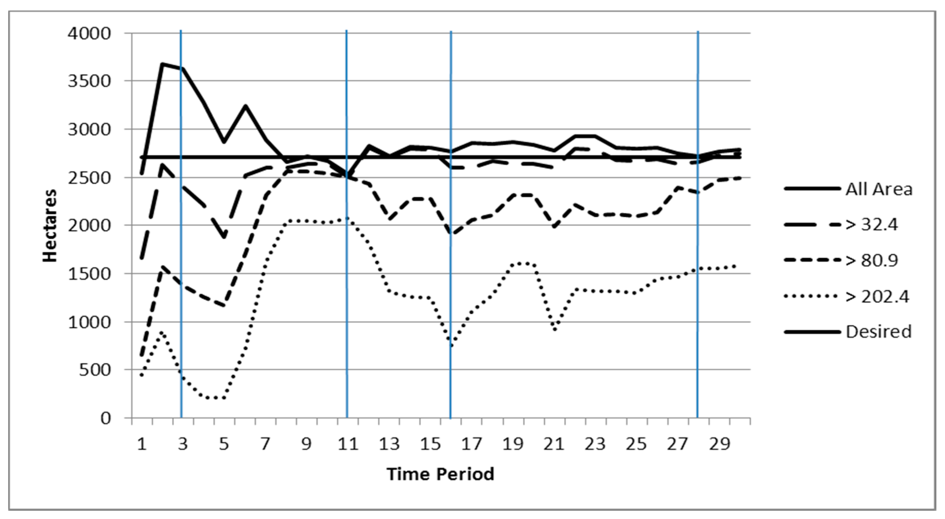
Patches are also measured relative to the total area of habitat in patches of varying sizes, chosen to correspond with sizes cited in past studies. Total area in patches greater than 32.4 ha is the minimum suitable size described by Probst and Weinrich [14]. The 80.9 ha patch size is the management standard suggested by Probst [12]. Finally, the 202.4 ha patch size is the historic occupation described by Probst and Weinrich [14], where 77% of the singing males were found in patches larger than 200 ha from 1979 to 1989.
Early periods have the most amount of habitat in patches less than the minimum suitable size (area between the “All Area” and “32.4” lines in Figure 8). The period 1–5 amounts are heavily influenced by the current habitat arrangement on the landscape. In these periods, 33% of the habitat in patches less than 32.4 ha patches. Later periods have less total habitat, but the area in patches greater than 32.4 ha is increased to 91% or more in periods 7–30 (Figure 8). Arguably the best performing period of the 2226 scenario is period 11. Period 11 has the highest level of area in patches greater than 202.4 ha in both absolute and percentage terms (2077 ha, or 82% of the period 11 total). Notably, period 11 also has the least amount of total habitat of the constrained periods (6–30). Period 16 appears to have the poorest performance as it has the least amount of area in patches greater than 80.9 ha (69%) and 202.4 ha (28%) over periods 6–30.
Core area efficiency ratio (CR) is correlated with patch size. Higher core area efficiency ratios are associated with fewer, larger patches with more core area in each patch. The S3 2226 scenario has the smallest ratios in periods 1–6, the largest ratios in periods 7–12 and a long-term ratio that is lower than the maximum (Figure 9). The current CR on the landscape is 58%. After the influence of current habitat wanes beyond period 7, the ratio reaches a maximum of 87% in period 11 before dipping to a minimum of 77% in period 16. The long-term ratio (periods 25–30) generally stabilizes at about 81%. Contrast this with the B2 Total Habitat benchmark, where core area is not considered. In this Benchmark, the resulting CR is between 52% and 65%, similar to the current condition of the landscape.
The B3 Core Only benchmark indicates whether the presence of other desired conditions (constraints) of the forest plan negatively affect the ability to manage for core area. In this benchmark, the CR is higher than the S3 scenario in periods 7–16, but is lower in the longer term (periods 17–30). This may be explained by financial discounting that recognizes lower production costs in the short term. Stated another way, the increased CR of B3 in early periods is associated with less habitat overall arranged in larger patches, which is financially less costly than the S3 scenario. The advantages of higher CR become less pronounced in later decades. Both the S3 and B3 model runs outperform the B2 Total Habitat benchmark, which accounts only for the financial costs of habitat management without considering spatial arrangement (Figure 9). Figure 10 is included to show a visual contrast between the S3 and B2 runs at period 16.
3.5. Financial Costs of Kirtland’s Warbler Habitat
The third objective of this study was to explore the financial trade-offs associated with Kirtland’s warbler management. The net present value (NPV) cost of managing the 2711 ha of Kirtland’s warbler habitat described in the Hiawatha National forest Land Management Plan is approximately $4.82 million, a 46% reduction in value (the difference between the B1 and B2 scenarios, Table 2). Arranging the habitat into large patches costs an additional $1.18 million, a 12% reduction in value (the difference between S3 and B2, Table 2). This study also shows the financial costs of managing different levels of habitat core area. The additional 405 ha of core area between S1 and S2 comes at a cost of $1.65 million and the 405 ha between S2 and S3 costs $1.77 million. This suggests the per-area marginal cost of habitat is greater with more core area management.
One other note is that the B3 Core Only benchmark has the highest NPV estimate. Recall that this benchmark includes timber and core area constraints, but does not have constraints on other forest desired conditions for cover type and size. The B3 Core Only benchmark is useful for showing the spatial potential of the landscape for suitable habitat but is not particularly useful for comparing financial value since it does not adequately implement forest plan desired conditions.
4. Discussion
The financial costs of Kirtland’s warbler habitat management are large. This is not surprising given the forest’s assumption that habitat regeneration is nearly two times the cost of normal jack pine regeneration. The long-term financial cost of habitat is measured as the difference between the B1 and B2 benchmarks, which results in a 46% reduction in NPV (Table 2). Spatially arranging habitat into large blocks incurs an additional $1.18 million reduction in NPV (Table 2 B2 vs. S3) While this may seem to be a large trade-off in absolute terms, percentage wise, the S3 2226 scenario NPV is 88% of the B2 Total Habitat benchmark. Thus, most of the cost associated with total habitat ($6.82 million between B1 and B2) appears to be the actual costs of management activity (site preparation and planting), rather than the trade-offs associated with the spatial arrangement of that habitat. However, the $1.18 million cost incurred from the spatial arrangement of the activity is generally foregone timber value. Foregone timber value might have resulted from managing sites before or after their age of maximum value, managing low value sites that would have otherwise been left unmanaged, or from converting sites that would have generated better revenues as a different cover type. Another phenomenon encountered in this study is the increased marginal costs of managing additional habitat. The cost of the additional 405 ha of core area in S3 relative to S2 was more expensive than the additional 405 ha of S2 relative to S1. This indicates that the model is working efficiently to first identify the best habitat opportunities before scheduling more costly areas. This information can also be used by managers when deciding the level of habitat to include in a management plan. One metric this study does not explicitly explore is the impact on the expected species population associated with the habitats in these benchmarks and scenarios. While the local population is likely dependent on larger population trends and even wintering habitat [6], site or landscape-specific predictive models such as those of Nelson and Buech [40] could provide information to balance the population trade-offs with the financial trade-offs of spatially arranging that habitat on the landscape.
One facet of the forest-wide problem to potentially explore in the future is the broader spatial distribution of patches by planning period. This might address the observed phenomenon that new patches close to occupied patches are colonized at younger ages [15]. One might consider addressing this using proximity constraints where specific subforest areas have core area goals in each planning period. Subforests could be defined as planning areas that are small enough to allow early colonization between patches contained in each subforest, but they would likely be larger than planning areas for less mobile species or species in which physical connectivity between patches is a key concern. For example, the four outwash plains in this study could be subforests. One way to maintain flexibility in year-to-year habitat levels within a subforest without explicit constraints would be to use downward-sloping demand curves to define the value at each time period. Specifically, a low habitat production level for a subforest has a higher per unit value for core area to recognize the concept of scarcity. This type of approach is described and was applied successfully by DePellegrin et al. [41].
Another factor our study does not directly address is the risk of low habitat levels on the persistence of the species in the planning area. Two key assumptions in this study are that management is the only factor contributing to Kirtland’s warbler habitat creation and that the management schedule determined by the model will be implemented exactly as prescribed. In reality, it is likely even the best management strategy will be disrupted by natural disturbance, economic fluctuations, or other complicating factors that prevent full implementation. If the disruption is large enough, it could result in habitat levels that negatively impact the endemic species population on the Hiawatha National Forest. There are at least two possible responses to a potential disruption—over-compensate by creating more habitat than necessary or re-analyze the management response after the disruption occurs. Each of these has its trade-offs; over-compensation has an increased financial cost, and re-analysis results could take years before habitat recovers to desired levels. However, for the Hiawatha National Forest, which is outside the core range of the species, it is unlikely that time periods with low levels of suitable habitat will significantly affect the persistence of the species.
Properly functioning ecosystems can be a challenge to manage in contemporary settings. Naturally occurring fires are not as prominent on the landscape as they were historically, largely due to fire suppression [11]. Mechanical regeneration in the jack pine ecosystem can mimic the ecological function fires, but they should consider not only scale (total area), but also landscape pattern. While we did not explicitly compare the pattern produced by the core area model runs to natural landscape pattern, it stands to reason that Kirtland’s warbler population responds favorably to conditions that mimic natural patterns. Those conditions result in earlier and longer residence times and include larger patch size and proximity to occupied habitat [12,14]. Again, it is not explicitly part of this study, but it is also common for other species to benefit from landscapes arranged in natural patterns.
5. Conclusions
Results of this study indicate that using computer-aided management scheduling tools can be an effective way to evaluate the landscape potential and financial trade-offs associated with the spatial objectives of habitat management. Specifically, the 2226 scenario that considered core area in management design created similar amounts of total habitat with substantially larger, more compact patches than when core area was not considered. Clearly, developing and sustaining management schedules with large Kirtland’s warbler habitat patches like those developed using the model would be a challenge to forest managers. Furthermore, the planning horizon and management options used in this study helped identify existing areas of present or planned habitat that should be considered for conversion to cover types other than warbler habitat in the long-term. These opportunities are not always apparent or easy to conceptualize without the assistance of scheduling tools.
Results show that there are large costs incurred for managing for warbler habitat regardless of its spatial arrangement. Aggregating habitat into large, compact patches (patches that have associated core area) incurs more costs, but the increase is marginal relative to the straight financial investment of site preparation and planting to increased stocking levels. The reality of the large cost of Kirtland’s warbler breeding habitat only further emphasizes the importance that should be placed on making informed management decisions regarding where and when to invest in habitat management. When the cost of the habitat is high, perhaps managers should emphasize the quality of the habitat (e.g., amount of core area) just as much, if not more so, than the overall quantity of the habitat. With solid analysis, better investment decisions can be made that benefit the landowner, wildlife, and stakeholders.
Author Contributions
Conceptualization, E.H. and H.H.; methodology, E.H. and H.H.; software, E.H. and H.H.; formal analysis, E.H.; investigation, E.H.; resources, E.H. and H.H.; data curation, E.H.; writing—original draft preparation, E.H.; writing—review and editing, H.H.; visualization, E.H.; supervision, H.H.; project administration, E.H. All authors have read and agreed to the published version of the manuscript.
Funding
This research received no external funding.
Institutional Review Board Statement
Not applicable.
Informed Consent Statement
Not applicable.
Data Availability Statement
No data provided by this study.
Acknowledgments
Personnel and staff of the Hiawatha National Forest for data resources, model assumption information, and expertise on Kirtland’s Warbler management.
Conflicts of Interest
The authors declare no conflict of interest.
References
- Mayfield, H. The Kirtland’s Warbler; Cranbrook Institute of Science: Bloomfield Hills, MI, USA, 1960. [Google Scholar]
- US Fish and Wildlife Service. Kirtland’s Warbler (Dendroica kirtlandii) 5 Year Review: Summary and Evaluation; US Fish and Wildlife Service East Lansing Field Office: East Lansing, MI, USA, 2012.
- Byelich, J.; DeCapita, M.E.; Irvine, G.W.; Radtke, R.E.; Johnson, N.I.; Jones, W.R.; Mayfield, H.; Mahalak, W.J. Kirtland’s Warbler Recovery Plan; US Fish and Wildlife Service: Mio, MI, USA, 1976.
- Michigan Department of Natural Resources; US Fish and Wildlife Service; US Forest Service. Kirtland’s Warbler Breeding Range Conservation Plan; Michigan Department of Natural Resources: Lansing, MI, USA, 2015.
- Scott, M.J.; Goble, D.D.; Haines, A.M.; Wiens, J.A.; Neel, M.C. Conservation-reliant species and the future of conservation. Conserv. Lett. 2010, 3, 91–97. [Google Scholar] [CrossRef]
- Brown, D.J.; Ribic, C.A.; Donner, D.M.; Nelson, M.D.; Bocetti, C.I.; Sheffield, C.M.D. Using a full annual cycle model to evaluate long-term population viability of the conservation-reliant Kirtland’s warbler after successful recovery. J. Appl. Ecol. 2016, 54, 439–449. [Google Scholar] [CrossRef]
- US Fish and Wildlife Service. Final Post-Delisting Monitoring Plan for the Kirtland’s Warbler (Setophaga Kirtlandii); Michigan Ecological Services Field Office: East Lansing, MI, USA, 2019.
- Probst, J.R.; Bocetti, C.; Sjogren, S. Population increase in Kirtland’s warbler and summer range expansion to Wisconsin and Michigan’s Upper Peninsula, USA. Oryx 2003, 37, 365–373. [Google Scholar] [CrossRef] [Green Version]
- Richard, T. Confirmed occurrence and nesting of the Kirtland’s warbler at CFB Petawawa, Ontario: A first for Canada. Ont. Bird 2008, 26, 2–15. [Google Scholar]
- Trick, J.A.; Greveles, K.; Ditomasso, D.; Robaidek, J. The first Wisconsin nesting record of Kirtland’s warbler (Dendroica kirtlandii). Passeng. Pigeon 2008, 70, 93–102. [Google Scholar]
- Donner, D.M.; Ribic, C.A.; Probst, J.R. Male Kirtland’s Warblers’ patch-level response to landscape structure during periods of varying population size and habitat amounts. Forest Ecol. Manag. 2009, 258, 1093–1101. [Google Scholar] [CrossRef]
- Probst, J.R. Kirtland’s warbler breeding biology and habitat management. In Integrating Forest Management for Wildlife and Fish; North Central Forest Experiment Station: Minneapolis, MN, USA, 1988. [Google Scholar]
- Kashian, D.M.; Barnes, B.V.; Walker, W.S. Landscape ecosystems of northern Lower Michigan and the occurrence and management of the Kirtland’s warbler. For. Sci. 2003, 20, 140–159. [Google Scholar]
- Probst, J.R.; Weinrich, J. Relating Kirtland’s Warbler population to changing landscape composition and structure. Landsc. Ecol. 1993, 8, 257–271. [Google Scholar] [CrossRef]
- Donner, D.M.; Ribic, C.A.; Probst, J.R. Patch dynamics and the timing of colonization-abandonment events by male Kirtland’s Warblers in an early succession habitat. Biol. Conserv. 2010, 143, 1159–1167. [Google Scholar] [CrossRef]
- Kepler, C.B.; Irvine, G.W.; DeCapita, M.E.; Weinrich, J. The Conservation Management of Kirtland’s Warbler Dendroica kirtlandii. Bird Conserv. Intern. 1996, 6, 11–22. [Google Scholar] [CrossRef] [Green Version]
- Marshall, E.; Haight, R.; Homans, F. Incorporating Environmental Uncertainty into Species Management Decisions: Kirtland’s Warbler Habitat Management as a Case Study. Conserv. Biol. 1998, 76, 975–985. [Google Scholar] [CrossRef]
- Marshall, E.; Homans, F.; Haight, R. Exploring Strategies for Improving the Cost Effectiveness of Endangered Species Management: The Kirtland’s Warbler as a Case Study. Land Econ. 2000, 76, 462–473. [Google Scholar] [CrossRef]
- Donner, D.M.; Probst, J.R.; Ribic, C.A. Influence of habitat amount, arrangement, and use on population trend estimates of male Kirtland’s warblers. Landsc. Ecol. 2008, 23, 467–480. [Google Scholar] [CrossRef]
- Kangas, M.; Kurtilla, T.; Eyvindson, H.; Kangas, J. Decision Support for Forest Management, 2nd ed.; Springer Ingernational Publishing: Berlin, Germany, 2015; Volume 30, pp. 1–307. [Google Scholar]
- Andersson, D.; Eriksson, L.O. Effects of temporal aggregation in integrated strategic/tactical forest planning. For. Policy Econ. 2007, 9, 965–981. [Google Scholar] [CrossRef]
- Rau, V.; Burkhardt, C.; Dorninger, C.; Hjort, L.; Ibe, L.; Kebler, J.; Kristensen, A.; McRobert, W.; Holm, H.S.; Zimmerman, D.; et al. Temporal patterns in ecosystem services research: A review and three recommendations. Ambio 2019, 49, 1377–1393. [Google Scholar] [CrossRef]
- Bellman, R. The theory of dynamic programming. Bull. Am. Math.Soc. 1954, 60, 503–515. [Google Scholar] [CrossRef] [Green Version]
- Hoganson, H.M.; Borges, J.G. Using dynamic programming and overlapping subproblems to address adjacency in large harvest scheduling problems. For. Sci. 1998, 44, 526–538. [Google Scholar]
- Borges, J.; Hoganson, H.; Rose, D. Combining a decomposition strategy with dynamic programming to solve spatially constrained forest management scheduling problems. For. Sci. 1999, 45, 201–212. [Google Scholar]
- Hoganson, H.M.; Bixby, J.; Bergmann, S.; Borges, J.G. Large scale planning to address interior space production studies from northern minnesota. Silva Lusit. 2004, 12, 35–47. [Google Scholar]
- USDA Forest Service. Final Environmental Impact Statement for Forest Plan Revision; Chippewa National Forest Superior National Forest: Duluth, MN, USA, 2004.
- Wei, Y.; Hoganson, H.M. Tests of a Dynamic Programming-Based Heuristic for Scheduling Forest Core Area Production over Large Landscapes. For. Sci. 2008, 54, 367–380. [Google Scholar]
- Henderson, E.B.; Hoganson, H.M. A learning heuristic for integrating spatial and temporal detail in forest planning. Nat. Resour. Model. 2021, 34, e12299. [Google Scholar] [CrossRef]
- Hoganson, H.M.; Rose, D.W. A Simulation Approach for Optimal Timber Management Scheduling. For. Sci. 1984, 30, 220–238. [Google Scholar]
- Hoganson, H.M.; Bixby, J.; Bergmann, S. Scheduling Old Forest Interior Space and Timber Production: Three Large-Scale Test Cases Using the DPSpace Model to Integrate Economic and Ecological Objectives; Minnesota Forest Resources Council: St. Paul, MN, USA, 2003.
- Hoganson, H.M.; Wei, Y.; Hokans, R.H. Integrating spatial objectives into forest plans for Minnesota’s National Forests. In Systems Analysis in Forest Resources: Proceedings of the 2003 Symposium; Pacific Northwest Research Station: Seattle, WA, USA, 2005. [Google Scholar]
- Wei, Y.; Hoganson, H. Landscape impacts from valuing core area in national forest planning. For. Ecol. Manag. 2005, 218, 89–106. [Google Scholar] [CrossRef]
- Hoganson, H.; Borges, J.G.; Wei, Y. Coordinating Management Decisions of Neighboring Stands with Dynamic Programming. In Designing Green Landscapes; Springer: Berlin/Heidelberg, Germany, 2008; pp. 187–213. [Google Scholar]
- USDA Forest Service. Hiawatha National Forest 2006 Forest Plan; USDA Forest Service: Escanaba, MI, USA, 2006.
- Baskent, E.Z.; Jordan, G.A. Characterizing spatial structure of forest landscapes. Can. J. For. Res. 1995, 25, 1830–1849. [Google Scholar] [CrossRef]
- Heinonen, T.; Kurttila, M.; Pukkala, T. Possibilities to aggregate raster cells through spatial optimization in forest planning. Silve Fenn. 2007, 41, 89–103. [Google Scholar] [CrossRef] [Green Version]
- USDA Forest Service. Hiawatha National Forest Final Environmental Impact Statement Appendix I; Forest Service: Escanaba, MI, USA, 2006.
- McGarigal, K.; Marks, B.J. FRAGSTATS: Spatial Pattern Analysis Program for Quantifying Landscape Structure; Gen. Tech. Rep. PNW-GTR-351; U.S. Department of Agriculture, Forest Service, Pacific Northwest Research Station: Portland, OR, USA, 1995; 122p.
- Nelson, M.D.; Buech, R.R. A test of 3 models of Kirtland’s warbler habitat suitability. Wildl. Soc. Bull. 1996, 24, 89–97. [Google Scholar]
- Llorente, D.P.; Hoganson, H.; Campione, M.W.; Miller, S. Using a marginal value approach to integrate ecological and economic objectives across the Minnesota landscape. Forest 2018, 9, 434. [Google Scholar] [CrossRef] [Green Version]
Figure 1.
Michigan’s Upper Peninsula (eastern portion) including the Hiawatha National Forest proclamation boundary and glacial outwash plains with potential Kirtland’s warbler habitat.
Figure 1.
Michigan’s Upper Peninsula (eastern portion) including the Hiawatha National Forest proclamation boundary and glacial outwash plains with potential Kirtland’s warbler habitat.

Figure 2.
Buffering used to define core area. The area within the triangle will provide core area only when stands 1, 3 and 4 all meet the requirements for Kirtland’s warbler breeding habitat. Area within larger hexagon surrounding stand 1 depends on condition of stand 1 for producing core area. The 0.81 ha hexagons used in this study have an average buffer distance of 37 m; the distance between the boundary of stand 1 and the larger hexagon around it.

Figure 3.
Core area constraint satisfaction for the three scenarios in this study. Horizontal lines are the core area constraint levels.
Figure 3.
Core area constraint satisfaction for the three scenarios in this study. Horizontal lines are the core area constraint levels.

Figure 4.
Total Kirtland’s warbler habitat resulting from constraints on core area. The horizontal line represents 2711 ha of desired habitat as described by the forest plan. Vertical lines at periods 6 and 11 indicate extreme values of the S3 2226 scenario solution.
Figure 4.
Total Kirtland’s warbler habitat resulting from constraints on core area. The horizontal line represents 2711 ha of desired habitat as described by the forest plan. Vertical lines at periods 6 and 11 indicate extreme values of the S3 2226 scenario solution.

Figure 5.
Core habitat areas scheduled in all time periods of the S3 2226 scenario (13,856 ha) and existing habitat not scheduled (2819 ha) for long-term persistence. This Figure represents the habitat potential of the four outwash plains of the Hiawatha National forest (Figure 1), rearranged spatially to better fit in the figure.

Figure 6.
Area of Kirtland’s warbler habitat regeneration by time period in the S3 2226 scenario. The cyclical pattern largely corresponds with the large amount of similarly aged habitat currently on the landscape that does not need to be replaced for several time periods.
Figure 6.
Area of Kirtland’s warbler habitat regeneration by time period in the S3 2226 scenario. The cyclical pattern largely corresponds with the large amount of similarly aged habitat currently on the landscape that does not need to be replaced for several time periods.

Figure 7.
Results from S3 2226 scenario (2226 ha core area constraint) for select time periods. KW Habitat is currently at appropriate stocking levels between the ages of 6 and 16, and Future Habitat is currently between ages 0 and 6.
Figure 7.
Results from S3 2226 scenario (2226 ha core area constraint) for select time periods. KW Habitat is currently at appropriate stocking levels between the ages of 6 and 16, and Future Habitat is currently between ages 0 and 6.

Figure 8.
S3 2226 scenario—Kirtland’s warbler habitat area in patches of various minimum sizes relative to total area of habitat (desired and modeled). Vertical lines correspond to the time periods depicted in Figure 7.
Figure 8.
S3 2226 scenario—Kirtland’s warbler habitat area in patches of various minimum sizes relative to total area of habitat (desired and modeled). Vertical lines correspond to the time periods depicted in Figure 7.

Figure 9.
Core area efficiency ratios (CR) for the S3 2226 scenario and the B2 and B3 benchmark scenarios.
Figure 9.
Core area efficiency ratios (CR) for the S3 2226 scenario and the B2 and B3 benchmark scenarios.

Figure 10.
Period 16 core area efficiency ratios for S3 2226 scenario (77%) and B2 Total Habitat benchmark (56%).
Figure 10.
Period 16 core area efficiency ratios for S3 2226 scenario (77%) and B2 Total Habitat benchmark (56%).


Table 1.
Starting condition and general constraint levels used to represent multiple management objectives of the Hiawatha National Forest.
Table 1.
Starting condition and general constraint levels used to represent multiple management objectives of the Hiawatha National Forest.
| Constraint Set | Constraint Type | Constraint Level (ha) | Starting Condition (ha) |
|---|---|---|---|
| Red Pine all ages | Lower | 16,593 | 21,272 |
| Mature red pine | Lower | 11,129 | 11,162 |
| Openings | Lower | 4027 | 3937 |
| Openings | Upper | 4512 | 3937 |
| Regeneration < 10 | Upper | 8033 | 8107 * |
| Non-KW Age 0–2 | Upper | 809 | 1177 * |
* The first period constraint is not violated due to growth out of the age class.
Table 2.
Net present value (NPV) estimates for benchmarks and scenarios.
| Benchmark/ Scenario | Financial Value of Solution ($MM) | Forest-Wide Constraints | |||
|---|---|---|---|---|---|
| Non-KW Type and Size by Period | Timber Even-Flow | Total KW Age 6–16, 2711 ha by Period | KW Age 6–16, Core Area by Period | ||
| B1: No Habitat | 14.92 | X | X | ||
| B2: Total Habitat | 8.10 | X | X | X | |
| B3: Core Only | 16.33 | X | 2226 | ||
| S1: 1416 Core | 10.34 | X | X | 1416 | |
| S2: 1821 Core | 8.69 | X | X | 1821 | |
| S3: 2226 Core | 6.92 | X | X | 2226 | |
Publisher’s Note: MDPI stays neutral with regard to jurisdictional claims in published maps and institutional affiliations. |
© 2021 by the authors. Licensee MDPI, Basel, Switzerland. This article is an open access article distributed under the terms and conditions of the Creative Commons Attribution (CC BY) license (https://creativecommons.org/licenses/by/4.0/).
Share and Cite
MDPI and ACS Style
Henderson, E.; Hoganson, H. Spatially Explicit Kirtland’s Warbler Habitat Management Scheduling in Michigan’s Upper Peninsula. Forests 2021, 12, 1065. https://0-doi-org.brum.beds.ac.uk/10.3390/f12081065
AMA Style
Henderson E, Hoganson H. Spatially Explicit Kirtland’s Warbler Habitat Management Scheduling in Michigan’s Upper Peninsula. Forests. 2021; 12(8):1065. https://0-doi-org.brum.beds.ac.uk/10.3390/f12081065
Chicago/Turabian StyleHenderson, Eric, and Howard Hoganson. 2021. "Spatially Explicit Kirtland’s Warbler Habitat Management Scheduling in Michigan’s Upper Peninsula" Forests 12, no. 8: 1065. https://0-doi-org.brum.beds.ac.uk/10.3390/f12081065
Note that from the first issue of 2016, this journal uses article numbers instead of page numbers. See further details here.