Temporal and Spatial Characteristics of Soundscape Ecology in Urban Forest Areas and Its Landscape Spatial Influencing Factors

Abstract

We explored the spatial and temporal characteristics of the urban forest area soundscape by setting up monitoring points (70 × 70 m grid) covering the study area, recorded a total of 52 sound sources, and the results showed that: (1) The soundscape composition of the park is dominated by natural sounds and recreational sounds. (2) The diurnal variation of sound sources is opposite to that of temperature, 6:00–9:00 is the best time for the public to perceive birdsong, and after 18:00, the park is dominated by insect chirps. (3) The PSD (power spectral density) and the SDI (soundscape diversity index) of the park are greatly affected by public recreation behaviors, and some recreation behaviors may affect the vocal behavior of organisms such as birds. (4) Spaces with high canopy density can attract more birdsong and recreational sounds in summer, and the combination of “tree + lake” can attract more birdsong. Vegetation has a significant dampening effect on traffic sound. (5) Landscape spatial elements, such as the proportion of hard ground, sky, trees, and shrubs, have a significant impact on changes in the PSD, the SDI and different kinds of sound sources. The research results provide effective data support for improving the soundscape of urban forests.

1. Introduction

Urban forests are important places for the public to get a close experience with nature, and the ways to improve the quality of urban forest recreation have received increasing attention and become the focus of many scholars [1,2]. As the construction of urban forests has entered the stage of quality improvement, managers have shifted from the creation of visual landscapes to a comprehensive improvement of the sensory experience [3,4,5,6], and soundscape is an important part of the senses. Ecosystem sounds create a soundscape comprised of acoustic periodicities and frequencies emitted from the ecosystem’s biophysical entities. These sounds are acoustic signals that reflect the dynamics of biological, social, and physical systems of a landscape. Soundscape ecology is “the study of systematic relationships between humans, organisms, and their sonic environment”. As an important resource ranked only second to the visual landscape, the soundscape has gradually received attention in the optimization design of urban forests [7,8]. Understanding and making proper use of the sounds in the environment around us are directly related to the livability of living environments and the quality of life of residents.

The soundscape varies in different landscape spaces. Scholars have conducted various studies on urban forests and other public open spaces, which mainly focused on soundscape changes [9,10,11,12,13] and quality evaluation [14,15,16,17,18,19,20]. Ali Jahani et al. assessed the role of birdsong components in the psychological recovery of urban visitors and developed a decision support system as a practical tool [21]. Hong Xinchen et al. explored the impact of soundscape-driving factors on the perception of birdsong and established a perceived birdsongs model (PBM) that effectively simulated the process from soundscape information to perceived birdsongs in urban forests. The methodology developed could be useful for soundscape assessment and conservation in urban forests [22]. Liu Jiang et al. showed that landscape features greatly affect the public’s perception of soundscapes and human-made sounds dominate urban soundscapes in the time-space dimension, but birdsongs and certain geophysical sounds also play an important role in soundscape [23]. Hao Zezhou et al. studied the variation characteristics and influencing factors of birdsongs and insect chirps in urban forests, as well as analyzed the activity patterns of urban biomes based on soundscape records [24]. Scholars have achieved fruitful achievements in the protection of green space biodiversity, improvement of public recreational benefits, and the reduction in noise; however, the existing research mainly uses the soundwalk method or sets up monitoring points in typical recreational areas to collect and analyze the acoustic data, and therefore, the results of studies are of weak guiding significance to the whole park.

We record sounds autonomously at multiple places in the park throughout the day and providing a window on the ecological spatiotemporal continuum, thereby provide a tool to capture the data needed to assess ecological integrity over time. This survey was able to visualize temporal patterns of landscape acoustic signals throughout the day to examine changes in the soundscape over time. Our study uses Hot Spring Park, located in the core area of Fuzhou city, during the summer as an example. To provide references for the management and optimization of the public space soundscape in urban core areas, monitoring sites in Hot Spring Park were selected by dividing grids and we focused on solving the following problems: (1) identify the structural features of urban forest sound sources, (2) analyze the spatial and temporal variation characteristics of the park soundscape, and (3) explore the differences in soundscape characteristics and influencing factors of various landscape spaces.

2. Materials and Methods

2.1. Study Location

Fuzhou was awarded the title of the “Chinese National Forest City” in 2017 and the “National Forest Tourism Model City” in 2018. Hot Spring Park is located in the city center of the intersection of “Riding Greenway” and “Inner River Greenway” in Fuzhou, which belongs to the core of urban forest [25]. The Hot Spring Park covers an area of about 10 hm²(119°18′34″ E~119°18′55″ E, 26°5′43″ N~26°5′59″ N). The park contains high species richness, with over 2000 big trees and 200 kinds of plants being planted here, and contains dozens of plant community structures, such as palm forest, evergreen coniferous forest, evergreen broad-leaved forest and deciduous broad-leaved forest [26]. With the increase in development in the city, Hot Spring Park has become a place for exercise, leisure, and entertainment for the public. In recent years, Hot Spring Park has undergone continuous upgrades and transformations, which provides the possibility for future soundscape integration.

2.2. Soundscape Monitoring and Data Acquisition

2.2.1. Soundscape Monitoring

According to previous studies, the feasible distance between recording equipment is 100 m [27,28,29]. We divided Hot Spring Park into grids that were equally distanced at 70 × 70 m [27] and selected 31 monitoring points (Figure 1). After our pre-experiment in July 2021, we randomly selected 3 sunny and breezy days for acoustic data collection (contains the weekend) so that our experiment would be more consistent with the actual situation of the park soundscape. Monitoring points were collected by placing a Sony PCM-D100 recording device in the center of a grid; if the monitoring point was inaccessible, an appropriate offset was made. Sampling occurred between 6:00 and 22:00 (park opening hours), and the sampling frequency was set to 44,100 Hz. The data resolution is set to 16 bit and the audio format was WAV. After sampling, we randomly intercepted 2 min of sound files within one hour [11], and had an average of 992 min of sound clips per day.

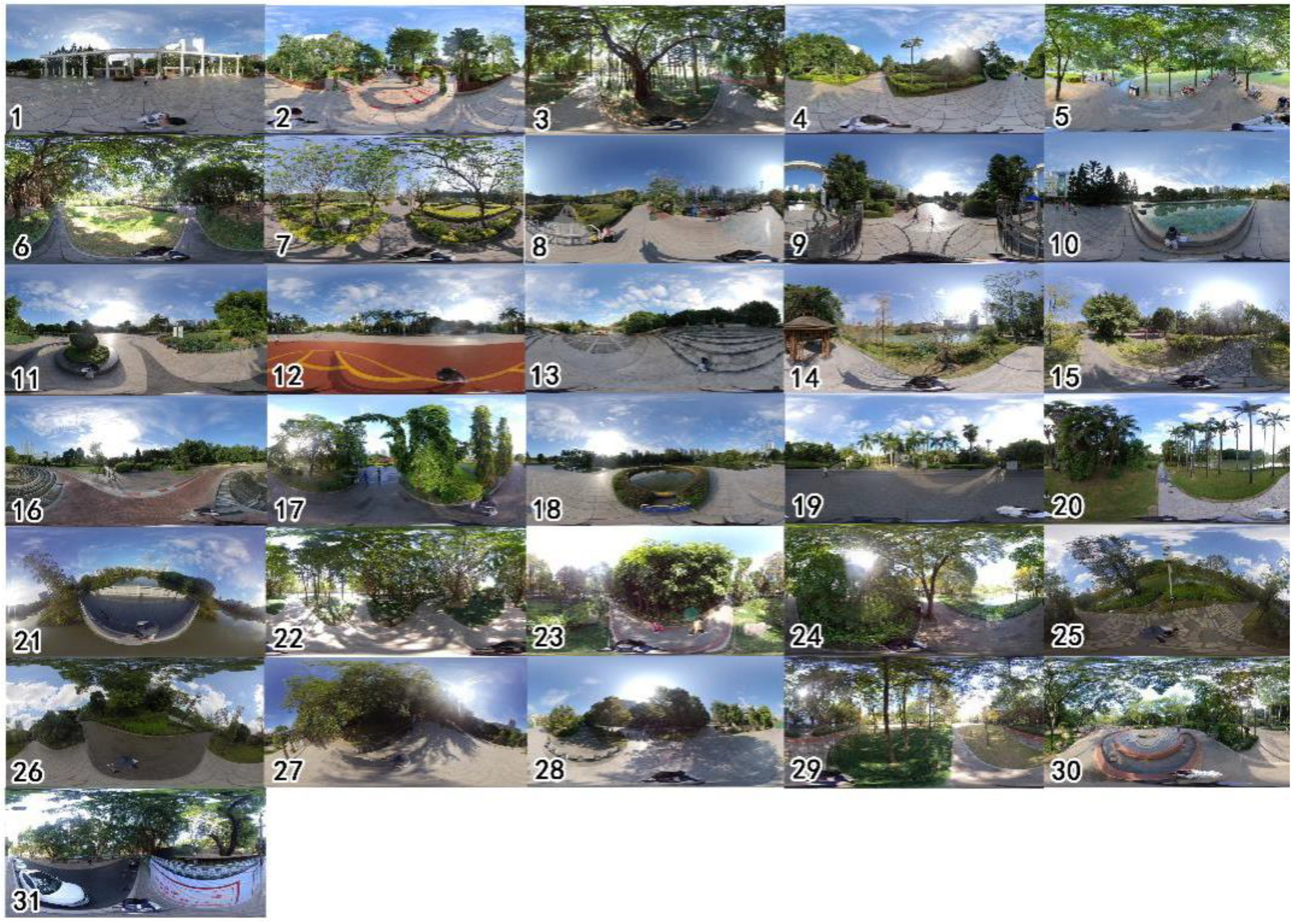
2.2.2. Panoramic Photos Collection

To analyze the landscape spatial characteristics of the monitoring site, a panoramic camera (Insta360 One X, panoramic image example shown in Figure 2) was placed during sound collection.

2.3. Data Processing and Analysis

2.3.1. Sound Source Analysis

To identify and classify the types of sound sources in urban parks, Adobe Audition was used in combination with spectrograms. Sound events can be visualized through the spectrogram, where brighter and more intense colors indicate a sound with greater power [30]. In our experiment, each acoustic signal appeared at the end of vocalization as one vocalization event [31] (Figure 3). In the statistics of audio, different kinds of sound sources in the same audio can be counted separately in frequency and time length, and sound types can overlap with each other.

2.3.2. Power Spectral Density

Different entities in the soundscape produce sounds at different frequencies [11]. Sound signals depict frequency on the vertical axis of the spectrum and time on the horizontal axis. The shading indicates the intensity (the power spectral density, PSD) of the sound signal at a particular frequency and time. Calculating the power spectral density can reflect the intensity of all the collected sound signals more objectively, and can also calculate the intensity of sound signals in different frequency intervals. The PSD, measured in w/kHz, was created by Welch in 1967 and represents the physical quantity of the power of an acoustic signal in relation to its frequency [32]. It is usually used to study acoustic signals of random vibration. The power of the sound can reflect the change of sound amplitude; that is, the greater the power, the greater the amplitude, the greater the amplitude, the greater the loudness, the greater the loudness, the stronger the sound is perceived by people [33]. Matlab was used to calculate the PSD in the range of 1–11 kHz to explore its temporal and spatial variations. In this study, the frequency of the sound sources observed was concentrated above 1 kHz, and data in the lowest interval, 0–1 kHz, was excluded as this can be largely attributed to human operation.

2.3.3. The Soundscape Diversity Index

The soundscape diversity index (SDI), used to evaluate the diversity of sound elements in the environment, was developed as an improved Simpson Diversity Index by scholars [34,35]. The main expression is as follows:

$$SDI=1-{\displaystyle \sum }_{i=1}^S{(\frac{n}{N})}^2$$

(1)

where n and N are the total number of perceived occurrences of a particular sound, I, and all sounds, S, in the soundscape sample, respectively. The SDI ranges between 0 and 1, and the greater the value, the more diverse the soundscape.

The SDI could “objectively” reflect soundscape characteristics and illustrates the overall soundscape perception characteristics [34], we calculated the SDI of each monitoring point to explore the spatial and temporal variation characteristics of park soundscape diversity.

2.3.4. Image Semantic Segmentation

To begin image semantic segmentation, a total of 770 pictures of Fuzhou city park were collected by camera (Contains both regular and panoramic photos) and randomly divided into training and test set according to the ratio of 10:1. Based on the classification of ADE20K dataset, images (including ordinary images and panoramic images) were manually annotated and input into DeeplabV3+ for training. The segmentation accuracy of the model reached 66.022% (MIoU = 66.022%), among which the segmentation accuracy of the water surface reached 84.53%. DeeplabV3+ is a mainstream network model in the field of image semantic segmentation, with multi-scale convolution layer and encoding-decoding dual modules [36]. It can achieve fine segmentation of the structure contained in the images [37]. As an encoding module, the DeeplabV3+ network can achieve hierarchical nested extraction of target features and multi-scale context information extraction, whereas the decoding module can integrate the low-level features and high-level abstract features generated in the DeeplabV3⁺ backbone network, and its structure is shown in Figure 4 [38]. Based on the DeepLabV3⁺ network structure, the urban park landscape labels are divided into 9 categories: water, trees, shrubs, ground cover, people, garden sketches, buildings, hard ground, and sky.

3. Results

3.1. Composition Characteristics of the Urban Forest Soundscape in Summer

Through the discrimination of audio files by manually listening combined with Adobe Audition software. A total of 52 types of sound sources were identified and then, based on the methods of previous studies, divided into four primary classifications: natural sound, traffic sound, management sound, and recreation sound (

Table 1. Classification of park sound source types.

Primary Classification	Expound	Secondary Classification	Sound Element
natural sound	produced by natural elements, and no interference from human activities.	plant sound	leaves
		animal sounds	birdsong, insects, pets, birds flapping wings, frogs
		natural phenomenon sound	wind
traffic sound	traffic sound around the park	traffic sound	car driving, car engine, tram driving, horn, airplane roaring, motorcycle, bus arrival, bus announcement, brake, siren, ambulance, bicycle bell
management sound	The sound of park management	maintenance sound	engine, steel plate, digging, electric drill, sweeping, door opening, trailer, beat, shovel, weed, fountain machinery, sprinkler
		device sound	park radio
recreation sound	sound from park activities and social interactions	activity sound	play badminton, clap and stomp, skateboard, jump rope, key shaking, slap the ball, portable radio, music, run and jump, walk,
		social sound	conversation, children playing, sing, reunion, cry, laugh, sneeze, cough, whistle, shout

.) [2,39,40,41]. The data of sound source types (including frequency and duration of different types of sound sources) in the monitoring points were averaged to represent the composition of sound sources in the park. A total of 60,527.6 s of sound source data were counted, with a total of 11,202 times. In terms of duration, natural sounds accounted for 28.51% of the overall, with birdsong and insect chirps being the majority (87.94%). Traffic sounds accounted for 9.63%, and consisted mainly of car driving sounds (78.49%). Management sounds accounted for 19.99%, with engine, fountain machinery and park radio sounds being the majority (88.90%). Recreational sounds accounted for 41.87%, and consisted mainly of music and conversation (70.13%). In terms of frequency, natural sounds accounted for 43.29% of the overall, with birdsong being the majority (96.74%); traffic sounds accounted for 5.27%; management sounds accounted for 10.40%; and recreational sounds accounted for 41.04%.

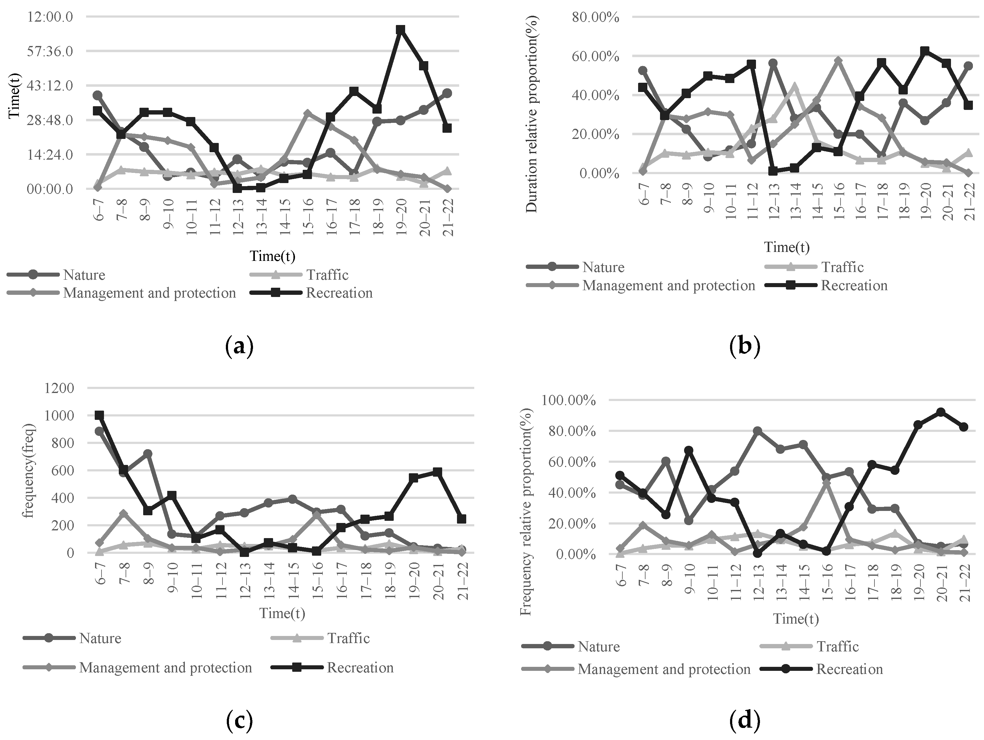
3.2. Diurnal Variation Characteristics of the Soundscape

3.2.1. Diurnal Variation Characteristics of Sound Sources

Overall, the soundscape presented a “U”-shaped change feature (Figure 5). Natural sounds occurred more frequently between 6:00 and 9:00 and lasted for a long time. Birdsong dominated the park soundscape, with Heron calls being the main bird soundscape present at noon. Natural sounds lasted longer at night and consisted mainly of insect chirps. Traffic sound dominated the park soundscape between 12:00 and 14:00 in duration. From 15:00 to 16:00, management sounds occupied a dominant position in the park soundscape, with the sounds of engines, park radio, sweeping, and mechanical fountains accounting for a large proportion. The sound of recreation appeared more frequently and lasted longer before 12:00 and after 16:00. The sounds of music and conversation in the morning made a greater contribution to the duration, and the sounds of people clapping, stomping, playing badminton, and walking made a greater contribution to the frequency. The sound of children playing, running and jumping accounted for a considerable proportion after 16:00.

3.2.2. Diurnal Variation Characteristics of the PSD

The PSD of the soundscape during the summer in Hot Spring Park were distributed between 0 and 1.2 w/kHz (Figure 6). Except for the sounds from birds, insects, horns, and brakes, most of the sound sources were included in the range of 1–3 kHz, mainly management and recreation sound. We found that power of the sound in the range of 1–3 kHz fluctuated and rose after sunrise. The peak in power between 16:00 and 17:00 and was greatly affected by the sounds of children playing, running, jumping, engine and wind. Between 20:00 and 22:00, the PSD decreased and gradually stabilized. The sound of birds, insects, and frogs were mainly in the 3–9 kHz frequency band. Some artificial sounds, such as horns, music, people playing badminton, clapping and stomping, would also reach frequencies above 3 kHz. Sound power in the 3–9 kHz band exhibited a very similar pattern to 1–3 kHz.

The relative proportion and diurnal variation characteristics of each frequency sound are shown in Figure 7. Sound power decreases with the increase in the frequency. The sound power of 1–3 kHz, mainly from recreation and management sound, accounted for more than 50% of the park’s power. The relative proportion of sound power fluctuated and rose after sunrise, and gradually decreased after reaching the maximum between 13:00 and 14:00 noon. However, the proportion of sound power above 3 kHz showed the opposite trend.

3.2.3. Diurnal Variation Characteristics of the SDI

The SDI was relatively high during the morning and night, and reached a low level between 12:00 and 15:00. After 15:00, the SDI gradually increased, and reached a peak of 0.827 between 17:00 and 18:00, and then gradually decreased once again (Figure 8).

3.3. Spatial Variation Characteristics of the Soundscape

3.3.1. Spatial Variation Characteristics of Soundscape Composition

The spatial variation characteristics of soundscape composition are shown in Figure 9. Natural sounds were evenly distributed in the park between 6:00 and 8:00. The frequency and duration of natural sounds were relatively low at monitoring points 12, 13, 27, 28 (square), and 29 (lawn along the street), these monitoring points experienced more recreational sounds during this period. Between 8:00 and 10:00, natural sounds were concentrated in the southeast area of the park, with monitoring point 14 near the lake experiencing the most sounds. Between 10:00 and 16:00, the frequency of natural sounds were highest in the children’s activity area, Ficus microcarpa by the lake, and the monitoring points with high canopy closure around them, mainly birdsong. The natural sound at the relatively open lakeside promenade in the southern part of the park and the monitoring points in the northern bamboo garden had a longer duration and consisted of mainly insect chirps. Between 16:00 and 18:00, the natural sounds at monitoring point 13 (Ficus microcarpa by the lake) and the southern lakeside promenade had high frequency and long duration. After 18:00, the frequency of natural sounds in most areas of the park decreased, and the vocal behavior of birds decreased., mainly insect chirps.

The frequency of traffic sound was higher at the park boundary. These monitoring points were mostly open spaces with single vegetation structure, were close to the main road and were greatly affected by traffic sound. The Aquarius Square had a high frequency of traffic sounds due to the entry of an external tram. Traffic sound affected an area up to 140 m from the park boundary, and the sound of horns could reach up to 210 m in the park. Monitoring points 16, 30, 26, and 27 were separated from surrounding roads by buildings or complex vegetation structure, even though the road was closer, the monitoring points were less affected by traffic sound.

Management sound was relatively random in the park. Between 6:00 and 12:00, the monitoring sites of the arched fountains have a longer sound duration, the sound of fountain machinery accounted for a large proportion. Between 14:00 and 18:00, the sound duration in the central square and the surrounding lake area was longer and consisted mainly of the engine. After 18:00, the main sound at the entrance of the park was the sound of the park radio.

Recreation sound was relatively evenly distributed between 6:00 and 8:00, and was either concentrated in the central square or a large hard area of the node. Areas that had a higher frequency of sound from badminton being played or the sound of clapping and stomping were Ficus microcarpa Garden, the south entrance square, the central Vase Square, and the north Bamboo Garden. Sound from the boulevard and children’s activity area lasted for a long time and mainly included the sound of music, children’s playing, and conversation. Between 8:00 and 16:00, the sound of music and conversation accounted for a large proportion, and their distribution was concentrated in a certain hard ground and tree covered environment. After 18:00, the sound of recreation covered the entire park again. The duration of the recreational sound increased significantly. The water features in the park did not play a significant role in attracting recreational sound.

3.3.2. Distribution Characteristics of the PSD

Figure 10 shows the distribution of the PSD in Hot Spring Park during the summer. The maximum sound power of the park (PSD = 1.09 w/kHz) was located at the riverside promenade on the east side of the park, which was affected by the beating sound of the external residential area, the sound of electric drills and the sound of traffic. Meanwhile, due to the open space, the monitoring point was located at the tuyere, which was greatly affected by the wind. The entrance on the north side of the park was close to the main road and was affected by traffic sounds such as cars driving and horns, the sound of park radio in entrance, and the sound of children playing during school closing time at dusk. The sounds of children playing also contributed a large amount of power, with a PSD of 0.8 w/kHz.

The PSD of monitoring point 12—Aquarius square, monitoring point 18—circular fountain and monitoring point 5—shady path were relatively high. In Aquarius square and circular fountain, the landscape space had the following characteristics: low basal plants, high basal constructions, without covering, both open space, plant enclosure was relatively low, and greatly affected by the sounds of engine and various recreational activities. Shady path in the basement of higher plants, the basal construction surface of low, high degree of vegetation cover, it is a semi-enclosed space, where the sound of children playing is of high power. In the southern part of the park, the sound energy was less than 0.2 W/kHz, and was mainly from the sounds of footsteps and conversation.

3.3.3. Distribution Characteristics of the SDI

As shown in Figure 10, monitoring points 12 and 13 were in open spaces with a large proportion of the basal construction and no coverage, which created a diverse sound environment for recreation. Monitoring points 2 and 4 were close to the north entrance of the park and were in the main passage for the public to enter the park. The sound of recreation was abundant at monitoring points 2 and 4. In addition, management sounds such as floor sweeping, were incorporated due to the daily management of the park. Monitoring point 24 was close to the lake, with complex vegetation and a superior natural acoustic environment. Monitoring point 31 was an open entrance plaza on the south side of the park, which was rich in recreational sound. Monitoring points 28 and 29 were close to the road and the traffic sound was rich. Meanwhile, monitoring point 28 was located next to the running track in the park, so the recreational sound was relatively rich and the SDI was high.

Monitoring point 14 was at the lakeside rest node based on the construction and water. The surrounding vegetation structure was simple, contained less area for movement, and the attraction of natural sound and recreational sound was insufficient. There was an artificial bird’s nest with prominent bird singing at monitoring point 17, and most of the public gathered to bird watch. The lack of other recreational behaviors led to a low SDI.

3.4. Influencing Factors of Landscape Space of the Soundscape

SPSS 26.0 software was used for correlation analysis and regression analysis to explore the relationship between landscape elements and the SDI, the PSD, and the frequency and duration of various sounds.

As shown in

Table 2. Correlation between the PSD, the SDI and the proportion of landscape spatial elements.

Indicators	Hard Ground Ratio	Building Ratio	Sky Ratio	Arbor Ratio	Tourists Ratio	Shrub Ratio	Ground Cover Ratio	garden Ornaments Ratio	Water Ratio
SDI	0.364 *	0.008	−0.069	0.147	−0.160	0.136	−0.002	0.233	−0.227
PSD	0.361 *	0.133	0.084	−0.272	0.032	−0.362 *	−0.062	0.122	0.008

* At the 0.05 level (two tailed), the correlation is significant.

., the proportion of hard ground had a significant positive correlation with the SDI and the PSD, while the proportion of shrubs had a significant negative correlation with the PSD. Through linear regression analysis, the listed landscape factors can explain 55.5% of the change in the PSD (R² = 0.555), and there was no collinearity between variables (VIF < 10), and the samples are independent of each other (DW = 2.336) (

Table 3. Summary of multiple linear regression models of the PSD and proportion of landscape elements.

Model	R	R2	Adjusted R2	Estimated Standard Error	Durbin-Watson
1	0.745 a	0.555	0.355	0.16873	2.336

R² reflects the variance explained by the regression equation as a percentage of the variance of the dependent variable. Durbin-Watson reflects autocorrelation of independent variables.

). Our results showed that the proportion of hard ground, sky, trees, and shrubs had a significant impact on the change in the PSD (p < 0.05) (

Table 4. Analysis of landscape elements affecting the PSD.

Model		Unstandardized Coefficients		Standardized Coefficients	t	Significance	Collinearity Statistics
		B	Standard Error	Beta			Tolerance	VIF
1	(constant)	0.766	0.355		2.157	0.043
	X1 Hard ground ratio	0.010	0.005	0.520	2.123	0.046	0.371	2.698
	X2 Building ratio	0.001	0.012	0.012	0.068	0.947	0.680	1.471
	X3 Sky ratio	−0.017	0.006	−1.161	−2.826	0.010	0.132	7.585
	X4 Arbor ratio	−0.015	0.005	−1.153	−3.066	0.006	0.157	6.359
	X5 Tourists ratio	−0.043	0.074	−0.115	−0.585	0.565	0.579	1.727
	X6 Shrub ratio	−0.031	0.013	−0.405	−2.420	0.025	0.793	1.261
	X7 Ground cover ratio	0.009	0.007	0.309	1.237	0.230	0.357	2.804
	X8 Garden ornaments ratio	0.234	0.231	0.187	1.015	0.322	0.657	1.521
	X9 Water ratio	0.012	0.007	0.317	1.670	0.110	0.617	1.620

). The greater the proportion of hard ground, the lower the proportion of sky, trees, and shrubs, the higher the PSD.

$$PSD=0.776+0.01\times X_1-0.031\times X_6$$

(2)

Listed landscape factors can explain 43.2% of the change in the SDI (R2 = 0.432), and the samples were independent of each other and there was no collinearity (VIF < 10, DW = 2.152) (

Table 5. Summary of multiple linear regression models of the SDI and proportion of landscape elements.

Model	R	R2	Adjusted R2	Estimated Standard Erro	Durbin-Watson
1	0.657 a	0.432	0.176	0.152	2.152

R² reflects the variance explained by the regression equation as a percentage of the variance of the dependent variable. Durbin-Watson reflects autocorrelation of independent variables.

). It was found that with the higher proportion of hard ground, the higher the diversity of the spatial soundscape and richer the soundscape (

Table 6. Analysis of landscape elements affecting the SDI.

Indicators	Unstandardized Coefficients		Standardized Coefficients	t	Significance	Collinearity Statistics
	B	Standard Error	Beta			Tolerance	VIF
(constant)	−0.053	0.320		−0.167	0.869
X1 Hard ground ratio	0.013	0.004	0.804	2.905	0.009	0.371	2.698
X2 Building ratio	0.008	0.010	0.167	0.818	0.423	0.680	1.471
X3 Sky ratio	0.005	0.005	0.426	0.917	0.370	0.132	7.585
X4 Arbor ratio	0.008	0.004	0.711	1.672	0.110	0.157	6.359
X5 Tourists ratio	−0.122	0.066	−0.409	−1.847	0.080	0.579	1.727
X6 Shrub ratio	0.013	0.012	0.210	1.110	0.280	0.793	1.261
X7 Ground cover ratio	0.006	0.007	0.280	0.992	0.333	0.357	2.804
X8 Garden ornaments ratio	−0.119	0.208	−0.119	−0.574	0.572	0.657	1.521
X9 Water ratio	0.000	0.006	0.017	0.079	0.938	0.617	1.620

).

$$SDI=-0.053+0.013\times X_1$$

(3)

Table 7. Correlation between various sound sources and the proportion of landscape space elements.

Indicators	Hard Ground Ratio	Building Ratio	Sky Ratio	Arbor Ratio	Tourists Ratio	Shrub Ratio	Ground Cover Ratio	Garden Ornaments Ratio	Water Ratio
Natural frequency	−0.537 **	−0.043	−0.109	0.157	−0.191	−0.079	0.318	0.018	0.287
Traffic frequency	−0.007	0.330	−0.301	0.217	0.154	0.023	0.249	−0.058	−0.233
Management frequency	−0.099	−0.213	−0.295	0.366 *	−0.030	0.521 **	0.173	0.413*	−0.060
Recreational frequency	−0.023	−0.427 *	−0.208	0.381 *	−0.299	−0.146	0.236	0.161	−0.032
Natural duration	−0.574 **	−0.432 *	−0.156	0.252	−0.443 *	0.002	0.572 **	−0.086	0.233
Traffic duration	−0.047	0.637 **	−0.370 *	0.314	0.218	−0.248	0.227	−0.243	−0.155
Management duration	0.285	0.193	0.424 *	−0.619 **	0.276	−0.190	−0.456 *	−0.203	−0.026
Recreational duration	−0.021	−0.250	−0.540 **	0.503 **	0.066	0.050	0.402 *	0.195	−0.305

* At the 0.05 level (two tailed), the correlation is significant; ** at the 0.01 level (two tailed), the correlation is significant.

further explores the relationship between the proportion of each landscape space element and various sound sources. Our results showed that, in terms of sound frequency, the proportion of hard ground had an extremely significant negative correlation with the frequency of natural sound. There was a significant negative correlation between the proportion of buildings and the frequency of recreational sound, while the proportion of trees has a significant positive correlation with the frequency of recreational sound. There was a significant positive correlation between the proportion of trees, shrubs, garden sketches and the frequency of management sound.

In terms of duration of vocalization, the proportion of hard ground, buildings, and people had a significant negative correlation with the duration of natural sound. Likewise, the proportion of ground cover had a significant positive correlation with the duration of natural sound. There was a significant positive correlation between the proportion of buildings and the duration of traffic sound, and a significant negative correlation between the proportion of sky and the duration of traffic sound. There was a significant positive correlation between the proportion of sky and the duration of the sound of management and protection, while the proportion of trees and ground cover had a significant negative correlation with the duration of the sound of management and protection. There was a significant negative correlation between the proportion of sky and the duration of recreational sound, but the proportion of trees and ground cover had a significant positive correlation with the duration of recreational sound.

4. Discussion

4.1. Diurnal Characteristics of the Soundscape

We found that natural sounds appeared most frequently between 6:00 and 9:00 and mainly consisted of birdsong. This verified the dawn chorus behavior of birds after sunrise [11,42]. However, the dusk chorus was not found in our monitoring, which may have been related to the different urban environments where the monitoring site was located. The increase in sound of recreation at dusk may also impact on the vocalization of birds. The long duration of nocturnal insect chirping was consistent with previous studies [43]. Traffic sounds dominated the park soundscape at noon as the high temperatures limited the frequency of natural and recreational sounds. Recreational sounds dominated the park soundscape before 12:00 and after 16:00, which was consistent with previous studies [44], and showed that the summer temperatures had a great influence on the recreational behavior of the public.

In the summer park, sounds in the 1–3 kHz frequency band accounted for more than 50% of the overall sound power of the park. The overall daily change was in the shape of “U”, with the valley appearing between 14:00 and 15:00 at noon. The diurnal variation characteristics of sound power were in good agreement with the temperature variation characteristics. In this study, playing, running, and jumping in the park during the late afternoon, when children were walking through or staying in the park after school, resulted in high levels of sound power in the park, and increased levels of sound power at dusk when the park engine and wind were affected. We found that the nighttime sound power of urban parks was lower, which was different from previous research results [31]. This could possibly be due to the prohibition of activities such as square dancing during the epidemic period, as well as children’s activities at night were distributed in fewer areas (mostly concentrated in children’s activity areas), the frequency and duration of children playing sound are low, and the power presented is small, which lead to lower sound power at night. Similarly, previous studies found that biological sounds were mainly distributed above 2 kHz [45,46], with vocal peaks appearing in the early morning [13]. We found that high-frequency and low-frequency sounds exhibited a similar diurnal variation pattern, we also found that many recreational sounds, such as the sound of people playing badminton, clapping, stomping, the sound of children playing, occupied the high-frequency band of biological sound and showed previously unseen higher power on the spectrogram, these recreational behaviors may have an impact on biological vocalizations. It was speculated that previous studies were mostly in the suburban forest and the sound of recreation had less influence on it. In terms of park soundscape diversity, the SDI showed a trend of higher in the morning and evening and lower in the noon, which was the same as the time distribution trend of recreational sound. The recreational behavior of the public had a great impact on the diversity of the park soundscape. Therefore, the SDI can be used as one of the indicators to measure the diversity of recreation behaviors in urban parks, and can be used as the basis for the evaluation of park recreation activities in subsequent studies.

4.2. Spatial Variation Characteristics of the Soundscape

The frequency and duration of natural sounds were lower in squares and parks along the street, but higher in forests with high canopy closure and lakeside forest areas. Our results confirmed that trees are an important factor in determining urban biodiversity [47,48,49], and that the physical attributes of tree, such as larger canopies and side branches, make big trees more attractive to birds [50]. Therefore, areas with high vegetation canopy closure and the combination of “big trees + lake water” can contribute to a suitable habitats for birds in summer, also enables the public to hear birdsong at noon in summer (such as egret and ardeola bacchus).

Traffic sounds had a higher frequency and longer duration at the park boundary. Most areas within 140 m from the park boundary were affected by traffic sounds, and vehicle horns were able to reach as far as 210 m in the park. The relatively open area close to the traffic road was influenced by the traffic sounds, and the open terrain was conducive to sound transmission, so the sound power is higher. By comparing monitoring points close to the road, we found that multi-layered plant configuration (especially shrub layer construction and utilization of plants with low branching points) and increased density of vegetation and structures can help reduce the noise of traffic outside. At the same time, previous studies have shown that structures can also affect the transmission of traffic sound, and the impact of traffic can be effectively reduced by placing structures on the side closest to the traffic road [51]. Increasing the density of façade elements near the road area helps to reduce the impact of traffic sound on the interior of the park.

The sounds of recreation during the day were mainly distributed at monitoring sites with high canopy closure. Since summer is different from the other seasons, light intensity and temperature were higher, and the spaces with higher canopy closure were most suitable for public activities [52]. Our study found that fountains and other water features did not bring significant attraction to recreational sounds during the opening hours of park’s water features. However, past studies have shown that the public has higher expectations for water sound [2], and it is speculated that the waterscape at the node does not produce pleasant soundscapes, such as water flow sound and water droplet sound [15]. At the same time, the waterscape in the park did not have hydrophilic functions, and the area of the venue provided for public activities was reduced. There were also fewer recreational facilities in the surrounding areas, which resulted in the lower frequency and duration of recreational sounds and the mechanical sound of the fountain in the square muffled the sound of water, therefore making the area less attractive to the public.

The SDI in the open space and the park entrance is higher, the recreational sounds in the two types of spaces is diverse, and the vegetation structure is rich around the lake to attract more natural sound. If the facilities in the site are strongly attractive to the public, there will be fewer recreational activities in the site, and the types of recreational sounds will be reduced. For example, the public will be attracted by the artificial bird nest in the field, and conduct birdwatching behavior, and only generate conversation sounds

4.3. Influence of Landscape Space Elements on the Soundscape

Among all landscape spatial elements, the larger the proportion of hard ground, the larger the soundscape power (the higher the PSD) and the higher the soundscape diversity (the higher the SDI). In parks, there are more types of recreational sounds than natural sounds, management sounds and traffic sounds, and the size of hard ground is an important factor related to public activities. In the two types of spaces with low proportion of trees and shrubs and low proportion of sky, the soundscape power is larger and the PSD is higher. It is found that spaces with low sky coverage (mostly covered by vegetation) will attract more recreational activities in summer, resulting in more recreational sounds and greater sound power. At the same time, in open spaces with large hard ground and low enclosed degree of trees and shrubs, it is more conducive to the public to carry out various activities and sound transmission, and the public will have a stronger perception of sound in this type of space. However, areas with large amounts of hard ground faced a reduction in natural sounds, and the increase in number of buildings and tourists will cause a decrease in natural sounds, especially birdsong. The lager the ground cover, the longer the natural, this kind of space was conducive to insect vocalizations. It was areas that were rich in ground-covering plants and shrubs that were conducive to insect habitat [39], and, as the park restricted visitors from entering the grassland, recreational behavior had less impact on insects. We found that recreation sounds increase when the proportion of trees and ground cover were larger, and the proportion of sky was smaller. We also found that the proportion of hard ground had no significant effect on the duration and frequency of recreational sounds, which further indicated that shaded environments and ventilation of the site were the main factors for the public to consider during summer recreation. We noticed that buildings, vegetation, and sky were commonly ignored factors in previous studies, but they, especially the proportion of sky, should be considered as key factors for future soundscape construction [23]. More space enclosed by buildings will reduce the frequency of recreational sound, and such space will be distributed in the boundary area of the park, which will restrict the recreation behavior of the public.

5. Conclusions

Our study drew the following main conclusions: (1) a total of 52 types of sound sources were identified in the forest environment of the urban core area in summer, and the park soundscape was dominated by natural sounds and recreational sounds. (2) Sound sources presented a “U”-shaped diurnal variation characteristic, and the variation characteristic was opposite to the temperature change. The best time for the public to perceive bird song is between 6:00 and 9:00; and after 18:00, the natural sound of the park is dominated by insect chirps. (3) The soundscape power and the soundscape diversity of the park are greatly affected by public recreation behaviors, and some recreation behaviors occupy the high-frequency band of biological vocalations, which may affect the vocal behavior of organisms such as birds (4) Building spaces with high canopy density can attract more birdsong and recreational sounds in summer, and the combination of “tree + lake” can attract more birdsong. As a negative sound, traffic sound can affect the space within 140 m, while horn sound can reach a further area. Enriching vegetation structure and increasing vegetation width can effectively shorten the influence range of traffic sound in urban forest. (5) In all kinds of landscape space, spaces with large hard ground and low degree of containment will attract public recreation, in such space the public perception of the soundscape will be more intense. In summer, the shade and ventilation condition of site is the main factor of public leisure to consider, this kind of space will attract more birds, at the same time, increase the cover area as well as forbid public access to the lawn is also conducive to insect habitat, increasing the proportion of insects chirping in the park. Compared to previous studies, the grid method was used to set monitoring points to refine the spatial variation characteristics of the soundscape in urban parks. The landscape spatial factors that affected the soundscape were determined based on factor analysis, and our research results provided effective data support for improving the soundscape of urban forests.

References

1. Liu, J.; Yan, Z.F.; Zhao, X. The Research of Soundscape Ecological Creativing Wisdom in Urban Relics Park. Chin. Landsc. Archit. 2018, 34, 73–75. [Google Scholar]
2. Zhang, Q.Y.; Hu, Y.; Li, D.D. Research on Soundscape of Tianjin Water Park Based on Soundwalls. Chin. Landsc. Archit. 2019, 35, 48–52. [Google Scholar]
3. Wang, Y.P.; Yin, C.H.; Ji, X.R.; Wang, Y. Experimental study on soundscape and audio-visual perception of urban historic district. J. Appl. Acoust. 2020, 39, 104–111. [Google Scholar]
4. Adams, M.; Cox, T.; Moore, G.; Croxford, B.; Refaee, M.; Sharples, S. Sustainable soundscapes: Noise policy and the urban experience. Urban Stud. 2006, 43, 2385–2398. [Google Scholar] [CrossRef]
5. Kang, J.; Zhang, M. Semantic differential analysis of the soundscape in urban open public spaces. Build. Environ. 2010, 45, 150–157. [Google Scholar] [CrossRef]
6. Pijanowski, B.C.; Villanueva-Rivera, L.J.; Dumyahn, S.L.; Farina, A.; Krause, B.L.; Napoletano, B.M.; Gage, S.H.; Nadia, P. Soundscape ecology: The science of sound in the landscape. BioScience 2011, 61, 203–216. [Google Scholar] [CrossRef] [Green Version]
7. Zhu, X.; Gao, M.; Zhao, W.; Ge, T. Does the presence of birdsongs improve perceived levels of mental restoration from park use? Experiments on parkways of Harbin Sun Island in China. Int. J. Environ. Res. Public Health 2020, 17, 2271. [Google Scholar] [CrossRef] [Green Version]
8. Ratcliffe, E.; Gatersleben, B.; Sowden, P.T. Associations with bird sounds: How do they relate to perceived restorative potential? J. Environ. Psychol. 2016, 47, 136–144. [Google Scholar] [CrossRef]
9. Joo, W.; Gage, S.H.; Kasten, E.P. Analysis and interpretation of variability in soundscapes along an urban–rural gradient. Landsc. Urban Plan. 2011, 103, 259–276. [Google Scholar] [CrossRef]
10. Alexandra, R.; Amandine, G.; Sandrine, P.; Philippe, G.; Philippe, G.; Jérôme, S. Temporal and spatial variability of animal sound within a neotropical forest. Ecol. Inform. 2014, 21, 133–143. [Google Scholar]
11. Stuart, H.G.; Anne, C.A. Visualization of temporal change in soundscape power of a Michigan lake habitat over a 4-year period. Ecol. Inform. 2014, 21, 100–109. [Google Scholar]
12. de Camargo, U.; Roslin, T.; Ovaskainen, O. Spatio-temporal scaling of biodiversity in acoustic tropical bird communities. Ecography 2019, 42, 1936–1947. [Google Scholar] [CrossRef] [Green Version]
13. Zhao, Y.L.; Bai, Z.T.; Wang, C.; Yin, L.Q.; Sun, Z.K.; Zhang, C.; Sun, R.L.; Xu, S.; Bian, Q.; Sun, B.Q. Urban parks soundscape and its relationship with vegetation structure: A pilot study. Acta Ecol. Sin. 2021, 41, 8040–8051. [Google Scholar]
14. Hong, X.C.; Wang, X.; Duan, R.; Zhang, H.; Chi, M.W.; Lan, S.R. Evaluation of soundscape preference in forest park based on soundwalk approach. Tech. Acoust. 2018, 37, 584–588. [Google Scholar]
15. Hong, X.C.; Lin, Z.Y.; Zhu, L.Y.; Lan, S.R. Research on Evaluation Index Selection of the Acoustic Environment of Suburban Forest Parks. For. Resour. Manag. 2016, 28, 116–120. [Google Scholar]
16. Guo, X.; Liu, J.; Christian, A.; Hong, X.C. Audio-visual interaction and visitor characteristics affect perceived soundscape restorativeness: Case study in five parks in China. Urban For. Urban Green. 2022, 77, 127738. [Google Scholar] [CrossRef]
17. Liu, J.; Yang, L.; Zhang, X.W. Research on the Relationship between Soundscape Perception and Landscape Evaluation in Historical Block: A Case Study in the Three Lanes and Seven Alleys in Fuzhou. Chin. Landsc. Archit. 2019, 35, 35–39. [Google Scholar]
18. Hong, X.C.; Wang, G.Y.; Liu, J.; Dang, E. Perceived Loudness Sensitivity Influenced by Brightness in Urban Forests: A Comparison When Eyes Were Opened and Closed. Forests 2020, 11, 1242. [Google Scholar] [CrossRef]
19. Hong, X.C.; Zhu, Z.P.; Liu, J.; Geng, D.H.; Wang, G.Y.; Lan, S.R. Perceived Occurrences of Soundscape Influencing Pleasantness in Urban Forests: A Comparison of Broad-Leaved and Coniferous Forests. Sustainability 2019, 11, 4789. [Google Scholar] [CrossRef]
20. Xu, X.Q.; Wu, H. Audio-visual interactions enhance soundscape perception in China’s protected areas. Urban For. Urban Green. 2021, 61, 127090. [Google Scholar] [CrossRef]
21. Jahani, A.; Kalantary, S.; Alitavoli, A. An Application of Artificial Intelligence Techniques in Prediction of Birds Soundscape Impact on Tourists’ Mental Restoration in Natural Urban Areas. Urban For. Urban Green. 2021, 61, 127088. [Google Scholar] [CrossRef]
22. Hong, X.C.; Wang, G.Y.; Liu, J.; Song, L.; Wu, E.T.Y. Modeling the impact of soundscape drivers on perceived birdsongs in urban forests. J. Clean. Prod. 2021, 292, 125315. [Google Scholar] [CrossRef]
23. Liu, J.; Kang, J.; Luo, T.; Behm, H.; Coppack, T. Spatiotemporal variability of soundscapes in a multiple functional urban area. Landsc. Urban Plan 2013, 115, 1–9. [Google Scholar] [CrossRef]
24. Hao, Z.Z.; Wang, C.; Pei, C.N.; Xu, X.H.; Zhang, C.; Duan, W.J.; Wang, Z.Y. Diversity of Soundscape in Three Urban Forests in Spring, Shenzhen. Sci. Silvae Sin. 2020, 56, 184–192. [Google Scholar]
25. Zhang, Y.Q. The Study on the Hot Spring Park Soundscape Design in Fuzhou; Fujian Agriculture and Forestry University: Fuzhou, China, 2017. [Google Scholar]
26. Lin, Z. Characters of Communities and Ecological Evaluation in Fuzhou Park Greenlands—Taking Five Parks for Example; Fujian Agriculture and Forestry University: Fuzhou, China, 2010. [Google Scholar]
27. Hao, Z.; Wang, C.; Sun, Z.; van den Bosch, C.K.; Zhao, D.; Sun, B.; Xu, X.; Bian, Q.; Bai, Z.; Wei, K.; et al. Soundscape mapping for spatial-temporal estimate on bird activities in urban forests. Urban For. Urban Green. 2020, 57, 126822. [Google Scholar] [CrossRef]
28. Zhang, G.Y. Application of Soundscape Mapping Technology in Soundscape Optimization of Urban Open Space: A Case Study in Beijing Park; Shenyang Jianzhu University: Shenyang, China, 2020. [Google Scholar]
29. Hu, J.; Ge, J.; Li, D.H. Analysis and construction of soundscape mapping based on GIS—A case of orioles singing in willows parks, Hangzhou. J. Zhejiang Univ. (Eng. Sicence) 2015, 49, 1295–1304. [Google Scholar]
30. Timothy, C.M.; Stuart, H.G.; John, M.M.; Falk, H. Temporal and spatial variation of a winter soundscape in south-central Alaska. Landsc. Ecol. 2016, 31, 1117–1137. [Google Scholar]
31. Bai, Z.T. Study of Characteristics of Anthrophony in Urban Parks in Beijing, China; Chinese Academy of Forestry: Beijing, China, 2020. [Google Scholar]
32. Welch, P. The use of fast Fourier transform for the estimation of power spectra: A method based on time averaging over short, modified periodograms. IEEE Trans. Audio Electroacoust. 1967, 15, 70–73. [Google Scholar] [CrossRef] [Green Version]
33. Bai, Z.T.; Wang, C.; Zhao, Y.L.; Hao, Z.Z.; Sun, Z.K. Characteristics and Temporal Variation of Spring Anthrophony in Urban Parks in Beijing. Chin. Landsc. Archit. 2021, 37, 99–104. [Google Scholar]
34. Liu, J.; Kang, J.; Behm, H.; Luo, T. Effects of landscape on soundscape perception: Soundwalks in city parks. Landsc. Urban Plan 2014, 123, 30–40. [Google Scholar] [CrossRef] [Green Version]
35. McGarigal, K.; Marks, B.J. Spatial pattern analysis program for quantifying landscape structure. In General Technical Report. PNW-GTR-351; US Department of Agriculture, Forest Service, Pacific Northwest Research Station: Corvallis, OR, USA, 1995; pp. 1–122. [Google Scholar]
36. Chen, L.C.; Zhu, Y.; Papandreou, G.; Schroff, F.; Adam, H. Encoder-Decoder with Atrous Separable Convolution for Semantic image Segmentation. In Proceedings of the European conference on computer vision (ECCV), Munich, Germany, 8–14 September 2018; pp. 801–818. [Google Scholar]
37. Li, L.; Wu, H.Y.; Zhang, T.Y. Constructing Semantic Map of Mobile Robots Based on Improved DeepLab V3+. Laser Optoelectron. Prog. 2022, 59, 255–265. [Google Scholar]
38. Liu, M.Y.; Liu, R.H.; Yao, Y.J.; Yu, Q.; Gao, Y.H.; Wang, R.; Sheng, B.; Jiang, L.X. Application of DeeplabV3+ network in ultrasonic image recognition of pediatric hip joint. Tech. Acoust. 2022, 41, 235–239. [Google Scholar]
39. Zhao, X.Z.; Mao, Y.; Hu, A. The characteristics of acoustic landscape in different landscape spaces of Huanhuaxi Park. J. Appl. Acoust. 2022, 41, 359–372. [Google Scholar]
40. Ge, J.; Lu, J.; Guo, H.F.; Li, H. Research on structure of soundscape in urban open spaces and its design method. J. Zhejiang Univ. (Eng. Sicence) 2006, 40, 1569–1573. [Google Scholar]
41. Hong, X.C.; Zhang, W.; Zhu, L.Y.; Lan, S.R. Soundscape risk degree evaluation in urban park. J. Appl. Acoust. 2016, 35, 539–546. [Google Scholar]
42. Depraetere, M.; Pavoine, S.; Jiguet, F.; Gasc, A.; Duvail, S.; Sueur, J. Monitoring animal diversity using acoustic indices: Implementation in a temperate woodland. Ecol. Indic. 2012, 13, 46–54. [Google Scholar] [CrossRef]
43. Hao, Z.Z. Dynamic Characteristics of Forest Soundscape in Three kinds of Urban Forest in Shenzhen Yuanshan Scenic Spot; Chinese Academy of Forestry: Beijing, China, 2017. [Google Scholar]
44. Yang, Y.J.; Sun, T.M.; Niu, X.K.; Sun, L.Q.; Wang, P.F. An SOPARC-Based Study of Summer Park Recreation Behavior—Taking Shuanglong Health Theme Park in Biyang County as an Example. J. Southwest Univ. (Nat. Sci. Ed.) 2021, 43, 173–180. [Google Scholar]
45. Sueur, J.; Farina, A.; Gasc, A.; Pieretti, N.; Pavoine, S. Acoustic indices for biodiversity assessment and landscape investigation. Acta Acust. United Acust. 2014, 100, 772–781. [Google Scholar] [CrossRef] [Green Version]
46. Mammides, C.; Goodale, E.; Dayananda, S.K.; Kang, L.; Chen, J. Do acoustic indices correlate with bird diversity? Insights from two biodiverse regions in Yunnan Province, south China. Ecol. Indic. 2017, 82, 470–477. [Google Scholar] [CrossRef]
47. Filazzola, A.; Shrestha, N.; MacIvor, J.S. The contribution of constructed green infrastructure to urban biodiversity: A synthesis and meta-analysis. J. Appl. Ecol. 2019, 56, 2131–2143. [Google Scholar] [CrossRef]
48. Stagoll, K.; Lindenmayer, D.B.; Knight, E.; Fischer, J.; Manning, A.D. Large trees are keystone structures in urban parks. Conserv. Lett. 2012, 5, 115–122. [Google Scholar] [CrossRef]
49. Yang, G.; Wang, Y.; Xu, J.; Ding, Y.Z.; Wu, S.Y.; Tang, H.M.; Li, H.Q.; Wang, X.M.; Ma, B.; Wang, Z.H. The influence of habitat types on bird community in urban parks. Acta Ecol. Sin. 2015, 35, 4186–4195. [Google Scholar]
50. Le Roux, D.S.; Ikin, K.; Lindenmayer, D.B.; Manning, A.D.; Gibbons, P. Single large or several small? Applying biogeographic principles to tree-level conservation and biodiversity offsets. Biol. Conserv. 2015, 191, 558–566. [Google Scholar] [CrossRef]
51. Meng, Q.; Kang, J. Study on Soundscapes in Urban Fringe Areas: Taking Tangchang Community Planning as an Example. City Plan. Rev. 2018, 42, 94–99. [Google Scholar]
52. Zhang, R.N.; Zhang, Y.; Liu, Y. Relationship between the landscape characteristics and the distribution of the soundscape in community parks: A case study of Lu Xun Park, Shenyang. J. Appl. Acoust. 2022, 41, 207–215. [Google Scholar]
Figure 1. Grid and location of monitoring points (the numbers represent our monitoring points).
Forests 13 01751 g001
Figure 2. Panoramic overview of 31 monitoring point.
Forests 13 01751 g002
Figure 3. Schematic diagram of sound spectrum recognition in each frequency band.
Forests 13 01751 g003
Figure 4. DeepLab V3+ model structure diagram [36].
Forests 13 01751 g004
Figure 5. Diurnal variation characteristics of duration, frequency and relative proportion of various sound sources; (a) diurnal variation of sound duration; (b) diurnal variation characteristics of relative proportion of sound duration; (c) diurnal variation of sound frequency; (d) diurnal variation characteristics of relative proportion of sound frequency.
Forests 13 01751 g005
Figure 6. Diurnal variation of acoustic power spectral density in 10 frequency ranges.
Forests 13 01751 g006
Figure 7. Daily variation of the relative proportion of sound power in each frequency band.
Forests 13 01751 g007
Figure 8. Characteristics of daily variation of the SDI.
Forests 13 01751 g008
Figure 9. Spatial distribution of natural, traffic, management, and recreational sounds.
Forests 13 01751 g009
Figure 10. (a) Spatial distribution characteristics of the PSD; (b) spatial distribution characteristics of the SDI.
Forests 13 01751 g010