Assessment of NO₂ Purification by Urban Forests Based on the i-Tree Eco Model: Case Study in Beijing, China

Abstract

Air quality issues caused by nitrogen dioxide (NO₂) have become increasingly serious in Chinese cities in recent years. As important urban green infrastructure, urban forests can mitigate gaseous nitrogen pollution by absorbing NO₂ through leaf gas exchange. This study investigated spatiotemporal variations in the NO₂ removal capacity of urban forests in Beijing city from 2014–2019, based on the i-Tree Eco deposition model. The results show that the annual removal capacity of administrative districts within Beijing city ranged from 14,910 to 17,747 tons, and the largest capacity (2684 tons) was found in the Fangshan district. The annual removal rate of NO₂ by urban forests in administrative districts within Beijing was estimated at between 0.50–1.60 g/m², reaching the highest (1.47 g/m²) in the Mengtougou district. The annual average absorption of NO₂ by urban forests can account for 0.14–2.60% of annual total atmospheric NO₂ and potentially reduce the NO₂ concentration by 0.10–0.34 µg/m³ on average. The results of a principal component analysis suggest that the distribution of urban forests in Beijing is not optimized to maximize their NO₂ removal capacity, being higher in suburban areas and lower in urban areas. This study provides insights into botanical NO₂ removal capacity in Beijing city to mitigate atmospheric N pollution, addressing the key role of urban forests in improving human wellbeing.

1. Introduction

China’s rapid urbanization has been accompanied by severe air pollution, particularly by nitrogen oxides (NO_x), which have become a major concern [1,2]. At the same time, the concentrations of typical air pollutants, including fine particulate matter (PM_2.5) and sulfur dioxide (SO₂), have been significantly reduced [3,4,5]. In some large cities, such as Beijing, the concentrations of NO_x and ground-surface ozone still remain at high levels due to the emission of traffic-related exhaust, thermal power generation, and regional atmospheric pollutant transport [6]. Large amounts of NO_x emissions may not only contribute to the photochemical production of aerosol and excessive atmospheric nitrogen deposition but may also induce the photochemical formation of ground-surface ozone [7,8]. Several studies have demonstrated that long-term exposure to NO_x and O₃ may increase the risk of respiratory and vascular disease in urban populations [9]. Therefore, exploring the sustainable mitigation of air pollutants in the urban environment is an urgent issue.

Terrestrial ecosystems are the most important N pools on the earth’s surface. The leaves of active plant organs are the main nitrogen sinks to store atmospheric nitrogen deposition [10]. Green infrastructures in urban environments, especially urban forests and green spaces, are widely recognized as providing ecological service functions to purify air pollutants [11,12,13]. Therefore, using green infrastructure in cities can be considered a cost-effective and nature-based approach to improve air quality. Previous studies have measured the uptake capacity of vegetation for NO₂ in indoor experiments based on a dynamic gas chamber method [14,15]. However, the uptake of NO₂ by urban forests in the urban environment is influenced by a combination of factors, including air pollutants concentrations, meteorological conditions, and the physiological features of plants [16]. Therefore, indoor measurements are difficult to extrapolate to represent the air pollutant uptake capacity of large-scale urban forests. Most studies have applied the UFORE model (urban forest effects model), and its enhanced version, the i-Tree Eco deposition model, to assess the air purification service supplied by urban forests [17,18,19]. The UFORE/i-Tree Eco model considers the removal of air pollutants by urban forests as a foliar deposition process of gaseous pollutants in multiple different boundary layers [19]. Several studies have quantified the NO₂ removal capacity of urban forests using the UFORE/i-Tree Eco model [19,20,21]. Studies using the UFORE/i-Tree Eco model have mostly focused on comparing differences in the purification capacity of urban forests in different cities and at different spatial scales. Most of these studies chose the growing season of trees in a year as the study’s period. However, fewer studies focused both on the spatial and temporal variability of the purification services of urban forests over a time series (Table S1).

Concentrations of NO_x in Beijing, the capital city of China, remain at high levels annually. Fuel combustion is the main source of gaseous nitrogen pollutants (mainly NO_x) emissions [6,22]. Yang, McBride, Zhou, and Sun [23] quantified air pollutant removal by urban forests in urban districts in Beijing and provided a cost-benefit analysis. They found that the species composition and canopy structure of trees in these urbanized areas are not conducive to maximizing NO₂ removal. The green cover in the city has increased from 47.4% to 48.5% during the period of 2014–2019 [24]. It is crucial to reappraise the potential NO₂ removal by urban forests in Beijing after significant green planting and tree replacement. The canopy growth of urban forests with artificial cultivation may theoretically contribute to biological NO₂ absorption [20]. However, few studies have examined how the social, economic, and ecological condition of sub-regions may affect the mitigation of NO₂ pollution by urban forests.

In this study, we addressed the questions above using ground-based monitoring datasets of daily NO₂ recordings between 2014 and 2019, focusing on all administrative districts (16 in total) in Beijing city. We first explored the spatial and temporal variations in NO₂ removal by urban forests in these districts during the period of 2014–2019, and then examined the relationships between socioeconomic factors and regional NO₂ removal by urban forests, finally assessing the NO₂ removal capacity in Beijing city by urban forests and their potential to mitigate atmospheric N pollution. By combining the socio-economic factors with the result of the i-Tree Eco deposition model, we can account for variations in urban activities and the absorption capacity of urban forest in different socioeconomic subregions [16]. This study attempts to provide information for city managers to optimize urban forest planning to maximize their NO₂ removal capacities.

2. Materials and Methods

2.1. Site Description

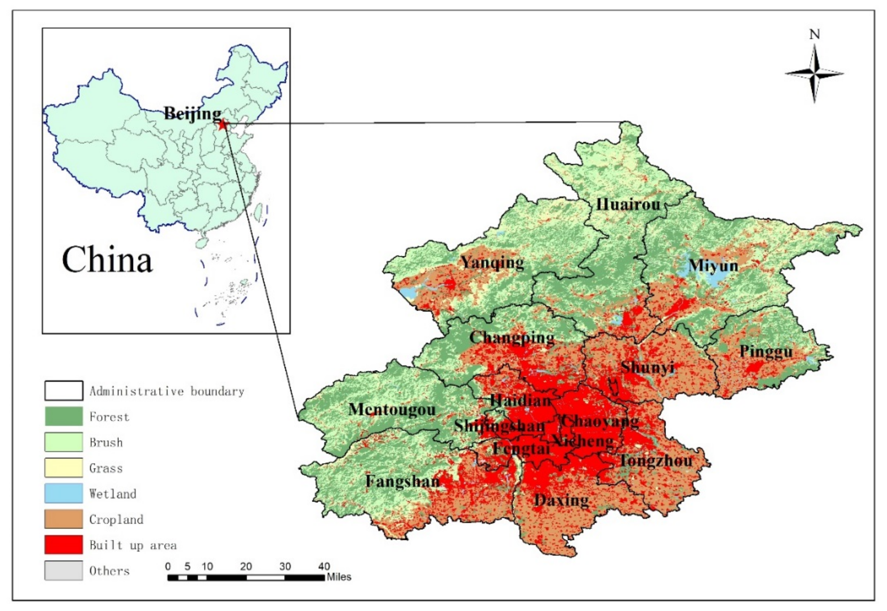
Beijing, with a total population of around 21 million, is located at the northwest of the North China Plain (39°56′ N, 116°20′ E), covering an area of approximately 16,411 km² and encompassing 16 administrative districts (Figure 1, Table S2) [25]. In recent years, the annual concentration of NO₂ in Beijing has increased and has reached concentrations ranging from 22.0 to 66.9 µg/m³ [26]. This increase is mainly attributed to the growth of NO₂ emissions from transportation and domestic sources [27].

There are around 55 species of trees planted in Beijing, and the main functional group of urban trees are deciduous broadleaf species and evergreen coniferous species, such as Populus tomentosa Carrière, Sophora japonica L., Fraxinus chinensis Roxb., Sabina chinensis L., and Pinus tabuliformis Carrière [28]. The green cover rate in Beijing has steadily increased from 47.4% to 48.5% during the period of 2014–2019 [24]. There is a gradient pattern for urban forests in Beijing, with significant differences in species and functional traits between urban and suburban districts [28,29].

2.2. Data Sources

Three types of data are used in this study. (1) Environmental and meteorological monitoring data. Hourly NO₂ concentration data from 2014–2019 were obtained from 34 air pollution monitoring stations. Most monitoring stations are located in the districts of central Beijing, and a few are located in the suburban area of the city (Figure S1). Five-minute meteorological data (wind speed, precipitation, and air temperature) from 2014–2019 were obtained from the meteorological stations located in the Beijing city area. (2) Remote sensing data. Leaf area index (LAI) data were acquired using the Landsat 8LAI remote sensing product at a spatial resolution of 30 m for the year 2019. Monthly LAI images from May to October (i.e., the common growing seasons for urban trees) in Beijing were aggregated and yielded a map of the average LAI values for the year 2019. Annual LAI for the period of 2014–2018 were estimated based on the ratio of regional green cover rate each year to that of 2019. (3) A large number of socioeconomic factors were used to examine the impact of urban development on NO₂ removal by urban trees, including green cover rate (Green), NO₂ concentrations (NO₂), particulate matter concentration (PM), fine particulate matter concentration (PM_2.5), SO₂ concentration (SO₂), environmental protection expenditure (Exp-Envir, log transformed), per capita disposable income (PCDI), total retail sales of consumer goods (TVSRC), gross domestic product (GDP), GDP of industry (GDPI), GDP of construction (GDPB), car ownership (CARS), total electricity consumption (ELC), total energy consumption (TEC), population (Pop), and population density (Pop-Den, log transformed). The data for most factors were obtained from the Beijing Municipal Bureau Statistics [25].

2.3. i-Tree Eco Deposition Model

To estimate the amount of NO₂ deposition on leaf canopy, we applied the spatial i-Tree Eco deposition model. We input the spatial distribution of pollutant concentrations and meteorological conditions, and then calculated NO₂ deposition flux F_d combined with hourly air pollutant concentrations as follows [19]:

F_d = V_d × C

(1)

where V_d (m/s) is the deposition velocity of NO₂ onto the leaves or within the vegetation canopy and C is the hourly concentration of NO₂. Deposition velocity was defined as the inverse of the sum of the aerodynamic (R_a), quasi-laminar boundary layer (R_b), and canopy resistance (R_c). The equation of the deposition velocity is shown below [30]:

V_d = 1/(R_a + R_b + R_c)

(2)

The aerodynamic resistance (R_a) is a function of windspeed under neutral conditions [31]:

$${\mathrm{R}}_{\mathrm{a}}=\mathrm{u}\left(\mathrm{z}\right)/{\mathrm{u}}_{*}^2$$

(3)

where u(z) is windspeed at height z and u_* is friction velocity. Friction velocity data were obtained from the previous study [32]. The quasi-laminar boundary layer resistance (R_b) is introduced to describe the resistance between fluid and deposition surface; it can be written as [33]:

$${\mathrm{R}}_{\mathrm{b}}=\frac{1}{{\mathrm{u}}_{*}}{\left(\frac{\mathrm{v}}{{\mathrm{D}}_{\mathrm{j}}}\right)}^{2/3}$$

(4)

where D_j is the diffusivity of air pollutants, v is the viscosity of air, and u_* is friction velocity. Canopy resistance R_c is introduced to describe the resistance effect of stomata gas exchange (R_st), leaf cuticle resistance (R_cut), and leaf mesophyll resistance (R_m) and can be expressed as [31,32]:

1/R_c = 1/(R_st + R_m) + 1/R_cu

(5)

Stomatal resistance depends on various factors such as canopy stomatal conductance, photosynthetically active radiation, air temperature, leaf water potential, etc. For simplicity of the calculation, the average stomatal resistance for different forest types was obtained from the published literature [14,15,32]. Leaf mesophyll resistance is related to the diffusion rate of pollutant gas in the mesophyll layer, the resistance value of leaf mesophyll for NO₂ was set to 100 s/m [34]. The cuticle resistance of evergreen coniferous forest, deciduous broadleaf forest, and mix forest was set to 5000 s/m, 7500 s/m, and 6250 m/s, respectively [34]. Based on Equations (2)–(5), the hourly NO₂ deposition velocity (Vd, m/s) was calculated for deciduous forests, evergreen coniferous forests, and mix forests (Table S3). For deciduous forests, the deposition velocity was set to 0 during the deciduous season. Finally, the spatial distribution of hourly NO₂ concentration was obtained from the interpolation of concentration data from the monitoring stations, and the hourly deposition flux per unit of leaf area calculated according to Equation (1) and Table S3. The annual removal rate Q_i and total NO₂ absorption capacity for each district over the whole year could be estimated from the hourly deposition flux and LAI of each district [35]:

$${\mathrm{Q}}_{\mathrm{i}}={\sum }_{\mathrm{j}=1}^{365}{ \mathrm{F}}_{\mathrm{ij}}\times {\mathrm{LAI}}_{\mathrm{i}}\times {\mathrm{T}}_{\mathrm{ij}}$$

(6)

Total NO₂ absorption capacity = Q_i × S_i

(7)

where F_ij is the hourly pollution removal flux for district i in day j, LAI_i is the average LAI value for district i, and T_ij is the sunlight hours for district i in day j. S_i is the area of district i.

To estimate the improvement effect of NO₂ removal by urban forests in Beijing, the hourly contribution of forests to NO₂ removal (ΔP_i) and the hourly air quality improvement (ΔC_i) were calculated as follows [35]:

$$\Delta P_t\left(\mathsf{\mu }\mathrm{g}\right)=\frac{{\mathrm{total} \mathrm{NO}}_2{ \mathrm{absorption} \mathrm{capacity}}_{\mathrm{i}}}{24\times 365}$$

(8)

$$\Delta C_i\left(\mathsf{\mu }\mathrm{g}/{\mathrm{m}}^3\right)=\frac{\Delta P_t}{BL\times A}$$

(9)

$$\Delta P_i\left(\%\right)=\frac{\Delta P_t}{C\times BL\times A}$$

(10)

$$\Delta C_i\left(\%\right)=\frac{\Delta P_t}{\Delta P_t+C\times BL\times A}$$

(11)

where ΔP_t (µg) is the hourly NO₂ removal by urban forests, ΔC_i ($\mathsf{\mu }\mathrm{g}/{\mathrm{m}}^3$) is the change in the NO₂ concentration due to the absorption effect of urban forests in district i, and ΔP_i (%) is the removal proportion of atmospheric NO₂ by vegetation absorption. ΔC_i (%) is the annual air quality improvement, C ($\mathsf{\mu }\mathrm{g}/{\mathrm{m}}^3$) is the measured annual concentration of NO₂, A (m²) is the area of the vegetation cover, and BL (m) is the annual mean boundary-layer height of Beijing, which was acquired from Climate Data Store (https://cds.climate.copernicus.eu/), with a temporal resolution of 1 month and a spatial resolution of 0.5° × 0.5°.

2.4. NO₂ Purification Deficit

The concept of ecological deficit has been widely applied to reflect the equilibrium of supply and demand of ecosystem services in a region. An ecological deficit occurs when the ecological capacity of a region is smaller than its ecological footprint [36,37]. To reflect whether the NO₂ emissions of 16 districts in Beijing exceed the removal capacity of urban forests, we propose the NO₂ purification deficit, which is calculated as follows:

$${\mathrm{NO}}_2{ \mathrm{Emissions}}_{\mathrm{i}}=\mathrm{Total} \mathrm{Emission} \times \frac{{\mathrm{Car}}_{\mathrm{i}}}{{\mathrm{Car}}_{\mathrm{total}}}$$

(12)

$$D_i={\mathrm{NO}}_2 {\mathrm{Emissions}}_{\mathrm{i}}-{\mathrm{Total} \mathrm{NO}}_2 {\mathrm{removal}}_{\mathrm{i}}$$

(13)

Total NO₂ emissions in Beijing are estimated as the total amount of nitrogen oxide emissions (since the nitric oxide is chemically instable) obtained from the Beijing Ecological-Environmental Statistical Annual Reports (Beijing Municipal Ecology and Environment Bureau, 2019). Traffic-related exhaust is the main NO₂ source and represents eight times the total amount from industrial, residential, and waste-treatment sources combined [27]. Therefore, we can calculate the approximate NO₂ emission of each district based on the regional proportions of motor vehicles. D_i is the NO₂ purification deficit of district i, estimated as the difference between traffic NO₂ emissions and NO₂ removal by trees in district i.

2.5. Statistical Analysis

Spatial heterogeneity of urban forest cover and of socioeconomic factors in the urban area may lead to large differences in the amount of NO₂ removal by urban forests in different socioeconomic regions [16]. To explore the variations of annual NO₂ absorption under different gradients of socioeconomic factors, we built a multiple regression model to capture the relationships between the amount of annual NO₂ absorption and relevant socioeconomic factors. We first built five competing models considering an increasing number of explanatory factors, following Garcia-Palacios, Gross, Gaitan, and Maestre [38]. The modeling process is as follows: (i) a “green only” model (only includes forest cover and NO₂ concentrations); (ii) an “environmental” model (includes all environmental factors); (iii) an “economic” model (the “environmental” model plus economic factors); (iv) an “energy” model (the “economic” model plus energy consumption factors); and (v) a “full” model (the “energy” model plus population factors, which includes all explanatory factors). We first used a model selection procedure based on corrected Akaike’s information criterion (AICc) and adjusted R² and variance inflation factor (VIF) to select the best-fitting model. For models i–v, factors with strong collinearity (VIF > 5) and factors that strongly influenced the AICc were removed during model selection. For the best model, a model-averaging procedure was performed based on the AICc and variance inflation factor (∆AICc < 5) to determine the parameter coefficients for the best final set of explanatory factors. We also evaluated the relative importance of explanatory factors in the final models. To calculate the relative effectiveness of each factor, all the parameters were standardized using Z-scores transformation before the analysis. The relative importance of four types of explanatory factors was calculated as follows: (1) population factors, (2) environmental factors, (3) economic factors, and (4) energy consumption. Assumptions of linear models (residual normality and variance homogeneity) were tested before model building. Some of the predictors were log-transformed to meet the linear assumptions of models. Then, we conducted a principal component analysis (PCA) to further characterize the gradient of NO₂ absorption by forests in the 16 districts. All the statistical analyses were performed using R 3.6.3 [39]. Model selection procedures were applied using the package ‘MuMIn’ [40]. We used the ‘vegan’ package to perform the PCA [41]. All the statistical graphs and maps were produced using ‘ggplot2’ [42] and ‘tmap’ packages [43].

3. Results

3.1. NO₂ Absorption Trends by Urban Forests during the Period of 2014–2019

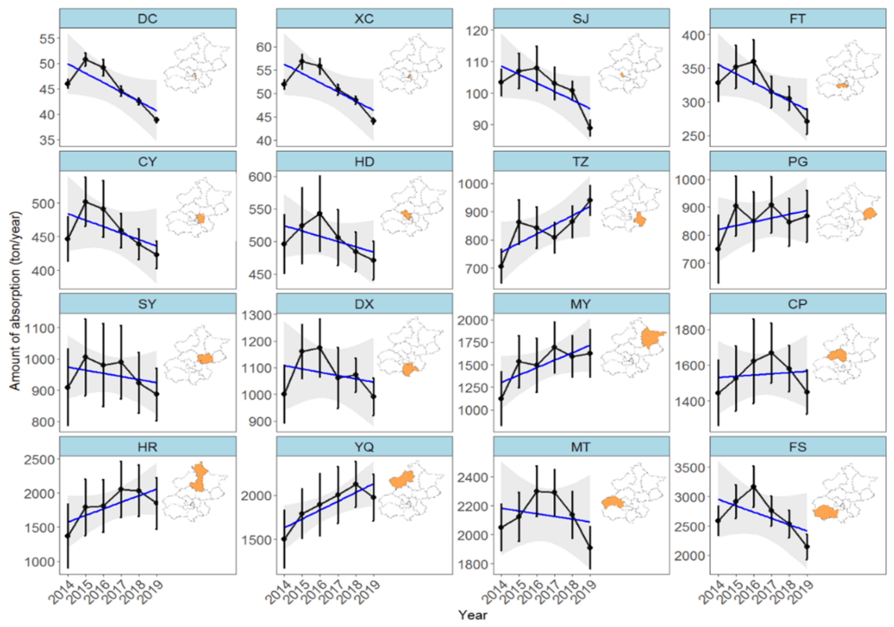
The variances in NO₂ absorptions by urban forests during the period of 2014–2019 based on the results of the i-Tree Eco deposition model are presented in Figure 2. The absorption amounts of six urban districts showed a decreasing trend during the period of 2014–2019, with some fluctuations. For the Dongcheng district (DC), Xicheng District (XC), and Chaoyang District (CY), the absorption of NO₂ by urban forests reached its highest value in 2015 in the following order: ZY = 501.9 tons (465.2–538.8 tons) > XC = 56.8 tons (55.3–58.5 tons) > DC = 50.8 tons (49.5–52.1 tons). Urban forests in the other three central urban districts reached their highest absorption values in 2016, in the following order: Haidian (HD) = 543.0 tons (485.5–600.6 tons) > Fengtai (FT) = 359.8 tons (327.2–392.4 tons) > Shijingshan (SJ) = 107.9 tons (100.9–114.8 tons). The absorption of NO₂ by urban forests was the lowest in 2019. The Haidian District (HD) had the highest absorption among the six urban districts, with a total of 471.2 tons (441.4–501.0 tons) in 2019. The lowest NO₂ absorption by urban forests among the six urban districts was the Dongcheng District (DC), with 38.9 tons (38.4–39.4 tons) in 2019. There were no consistent trends of NO₂ absorption by forests in the 10 districts located in the suburban area during the period of 2014–2019. An increasing trend of NO₂ absorption was found in the Tongzhou District (TZ, slope = 32.5, p = 0.26), Pinggu District (PG, slope = 13.6, p = 0.64), Miyun district (MY, slope = 82.9, p < 0.01), Huairou District (HR, slope = 96.7, p < 0.05), Yanqing District (YQ, slope = 99.6, p < 0.01), and Changping District (CP, slope = 6.8, p < 0.81). In contrast, for the Shunyi District (SY, slope = −9.9, p = 0.73), Daxing District (DX, slope = −12.3, p = 0.67), Mentougou District (MT, slope = −18.8, p = 0.51), and Fangshan District (FS, slope = −107.1, p < 0.01), the total absorption amount of NO₂ displayed a decreasing trend.

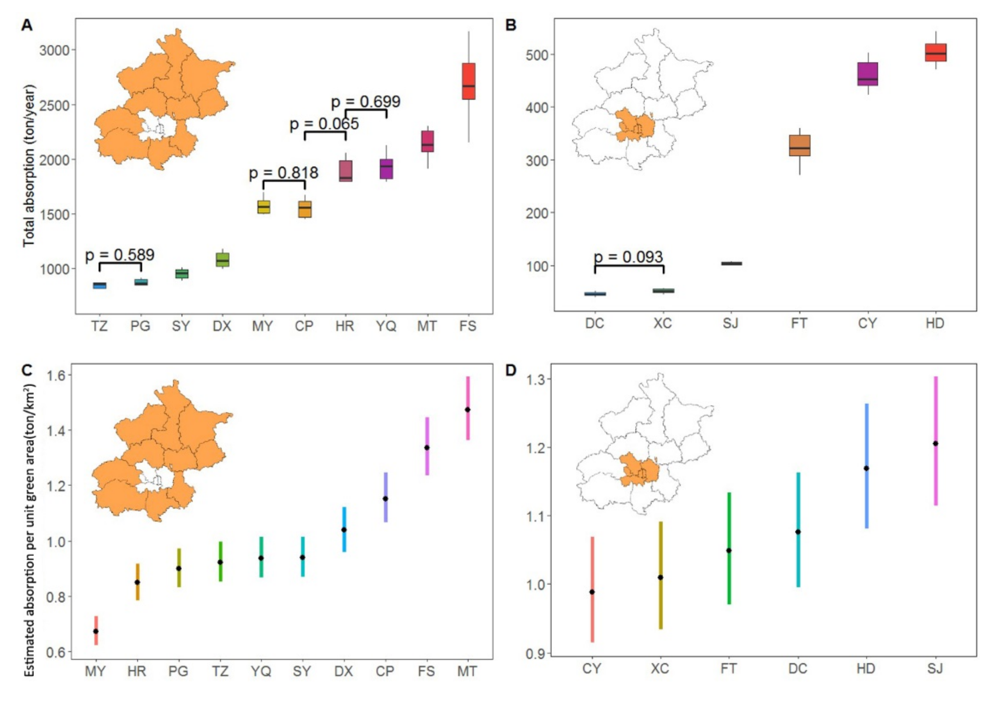
The average annual absorption in the 16 districts of Beijing over the study period varied greatly between suburban (10 districts) and urban areas (six districts), the average annual absorption in urban areas being significantly lower than in suburban areas (Figure 3A,B). The Haidian District had the highest average annual absorption (mean = 500.9 tons/year). The Dongcheng District had the lowest absorption, with an average 45.3 tons/year over the 6 years. The average annual absorption in the 10 suburban districts varied greatly in the following order: The Fangshan District (FS, 2684 tons/year) > Mentougou district (MT, 2136 tons/year) > Yanqing District (YQ, 1883 tons/year) > Huairou District (HR, 1818 tons/year) > Changping District (CP, 1549 tons/year) > Miyun District (MY, 1510 tons/year) > Daxing District (DX, 1077 tons/year) > Shunyi District (SY, 949 tons/year) > Pinggu District (PG, 855 tons/year) > Tongzhou District (TZ, 837 tons/year). There were also large differences in the absorption per unit of green area in 16 districts (Figure 3C,D), with the average absorption per unit of green area in the six urban districts being significantly higher than in the 10 suburban districts (urban districts = 1.08 ± 0.09 ton/km², suburban districts = 1.02 ± 0.24 ton/km², and p < 0.01). For the suburban areas, the highest NO₂ absorption rate of 1.47 ton/km² was found in the Mengtougou District (MT), while the Miyun (MY) District had the lowest absorption rate with 0.67 ton/km². The Shijingshan District had the highest absorption rate for urban districts, with 1.21 ton/km². The Chaoyang district (CY) had the lowest NO₂ absorption rate (0.99 ton/km²). In general, there was no consistent trend in the change in NO₂ absorption in the 16 districts of Beijing from 2014 to 2019. Annual absorption in the six urban districts showed a decreasing trend, and among the 10 suburban districts, six districts showed an increasing trend in absorption, while the annual total NO₂ absorption in the other four districts was decreasing. From the perspective of spatial distribution of NO₂ absorption, a large imbalance was found between the urban and suburban areas.

3.2. NO₂ Absorption Gradient between Urban Districts and Suburban Districts

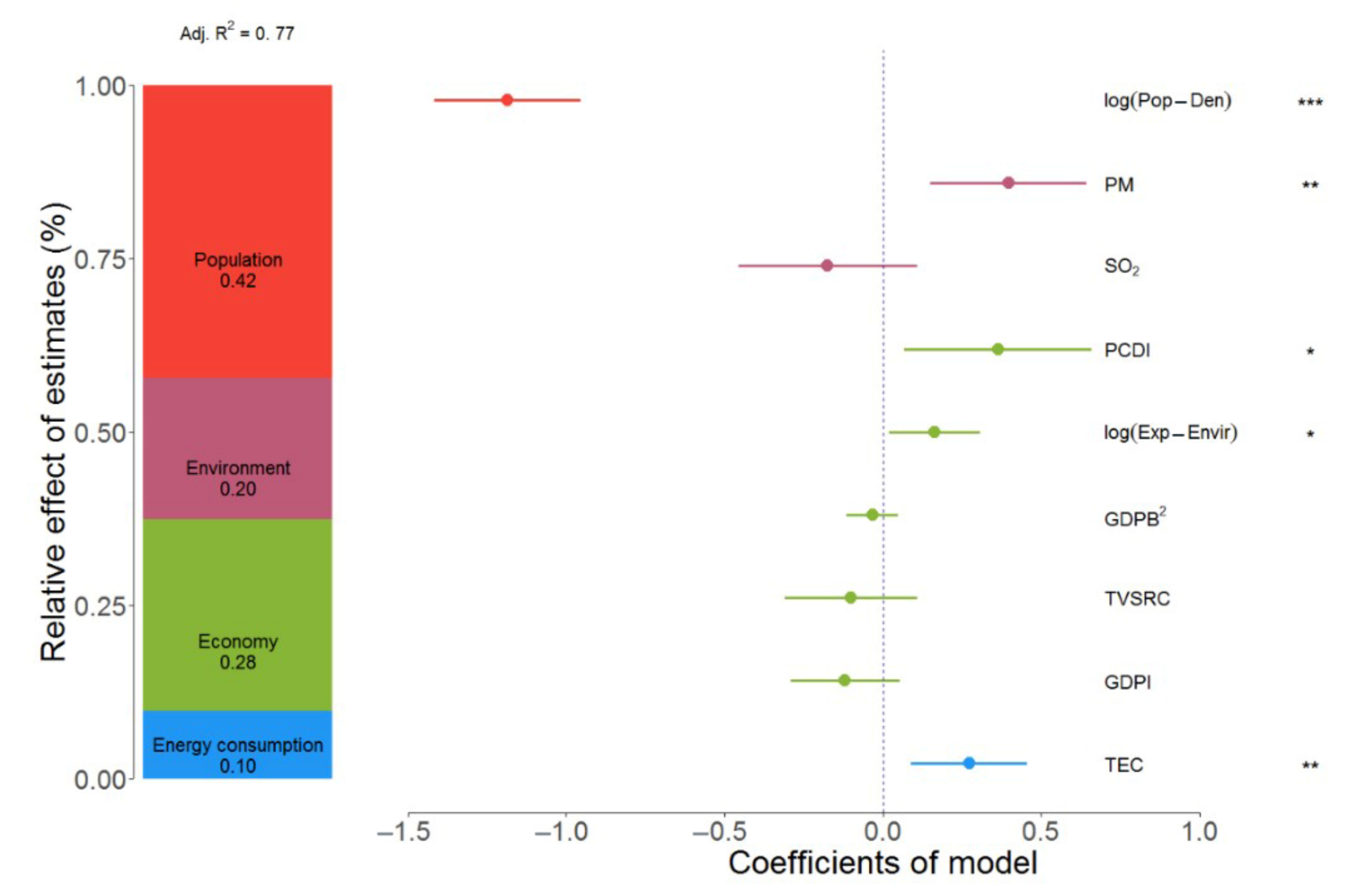
To explore the relationship between total annual NO₂ absorption and other factors in the 16 districts from 2014 to 2019, we selected 16 potential explanatory factors to build the regression models (Table S4, Table S5). These explanatory factors can be divided into four categories: environmental factors, economic factors, energy consumption factors, and population factors. After applying the model selection procedure, the final models included nine parameters. The coefficients of the parameters and their relative importance are displayed in Figure 4. The adjusted R² of the final model is 0.77, which explains a high proportion of the variance of annual NO₂ absorption. Among the four types of explanatory factors, the population factors were responsible for 42% of explained variance, followed by economic factors (28%), environmental factors (20%), and energy consumption factors (10%). We observed that the coefficients of population density (Pop-Den, log-transformed), PM concentration (PM), total retail sales of consumer goods (TVSRC), environmental protection expenditure (Exp-Env, log-transformed), and total energy consumption (TEC) were significant. The coefficient of population density was negative (−1.19, 95% confidence interval: −1.42 ~ −0.95), indicating that urban forests in high population density areas have a lower NO₂ absorption capacity than urban forests in low population density areas. This negative effect implies that urban areas with high population density may have lower NO₂ absorption due to lower green cover. We found positive coefficients for PM concentrations (0.40, 95% confidence interval: 0.15–0.64), indicating a positive correlation between PM concentration and NO₂ absorption, which may be explained by the existence of a positive correlation between PM concentration and NO₂ concentration (Spearman correlation = 0.84, p < 0.001). For the economic factors, the coefficient of environmental protection expenditures was positive (0.16, 95% CI: 0.02–0.31), suggesting that in those districts with higher environmental protection expenditures, urban forests tend to have a higher NO₂ absorption capacity. We also found that the parameter of total energy consumption (TEC) was positively correlated to annual absorption, which indicates that an increase in energy consumption leads to an increase in NO₂ emissions, and therefore, stimulates the capture of more NO₂ emissions by tree leaves.

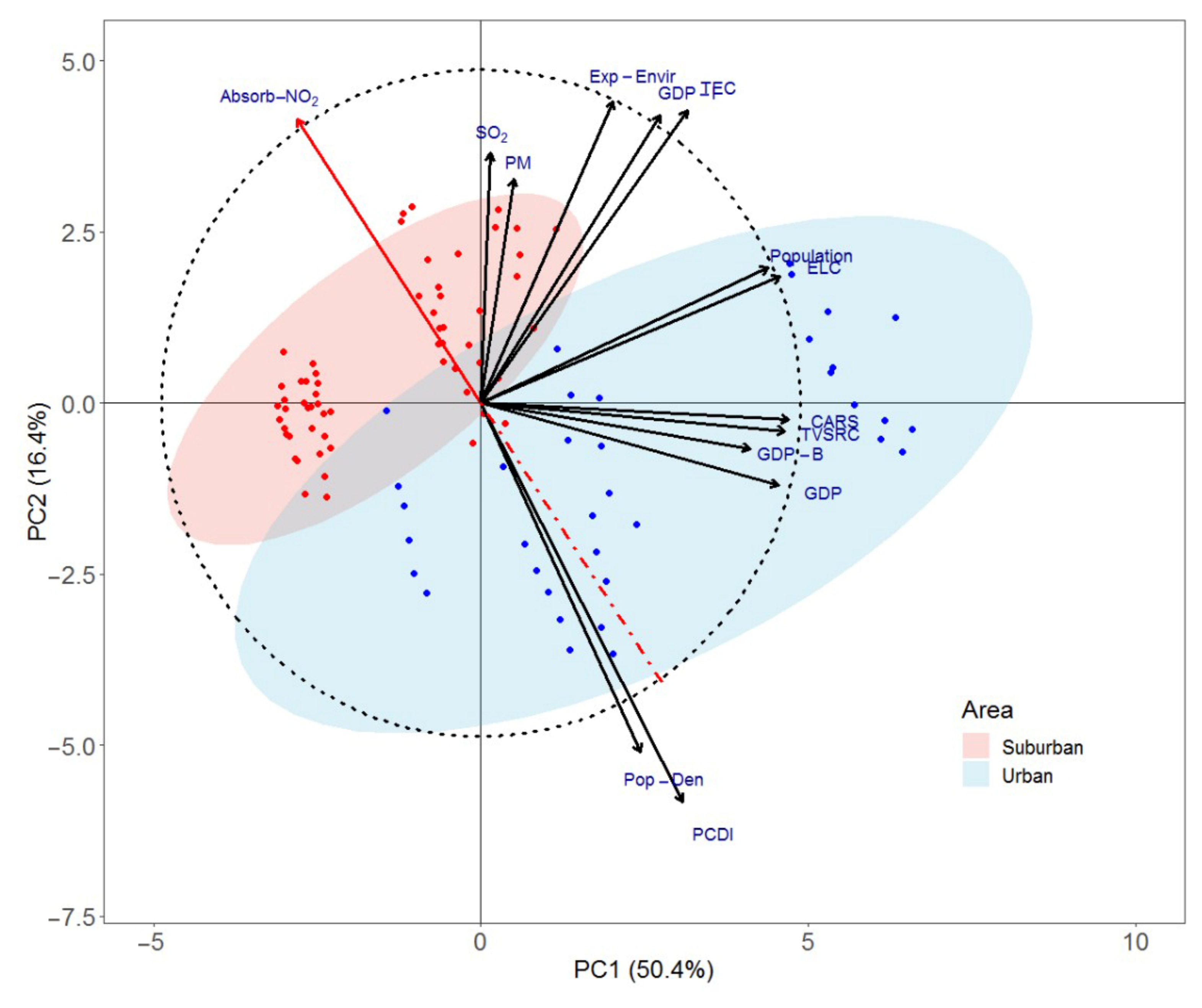
We conducted a principal component analysis (PCA) to further characterize the gradient of NO₂ absorption by forests in the 16 districts. Table S6 presents the top three principal components (PC) in terms of explained variance. The proportion of variance explained by the three principal components is 50.4%, 16.4%, and 14.9%, respectively. The cumulative variance proportion of the first two components is 66.8%, indicating that the variance of the data is mainly explained by the first two PCA components. The economic factors and energy consumption factors have high scores on the first principal component, which suggests that the first components mainly explain the variation of economic level and energy consumption in different districts. The second principal component has high scores for population factors and environmental factors, indicating that the variation of population and environmental factors in 16 districts are responsible for this component. The biplot (Figure 5) displays the ranking of annual NO₂ uptake and explanatory factors in the two principal components. From the perspective of correlations between explanatory factors and annual absorption amount, the correlation between annual NO₂ absorption (Absorb_NO₂) and SO₂ concentration and PM concentration and environmental protection expenditure is positive. However, the correlations between annual absorption amount and population density (Pop-Den), TVSRC, GDP, and car ownership are negative. From the perspective of results ranking, there is a clear clustering pattern between suburban districts (red points) and urban districts (blue points). The suburban districts with a high absorption amount are mostly clustered in the ranking axis area with low population density and lower per capita income, while the urban districts are mostly clustered in the ranking axis area with lower absorption amount, high population density, and high per capita income. Using the results of the PCA analysis, we further demonstrated the uneven distribution pattern of total NO₂ absorption by urban forests in the 16 districts of Beijing. In the urban area with high population density, urban forests provide much lower NO₂ absorption capacity than forests in suburban areas with lower population density.

3.3. Contribution of NO₂ Absorption by Urban Vegetation to N Pollution Mitigation

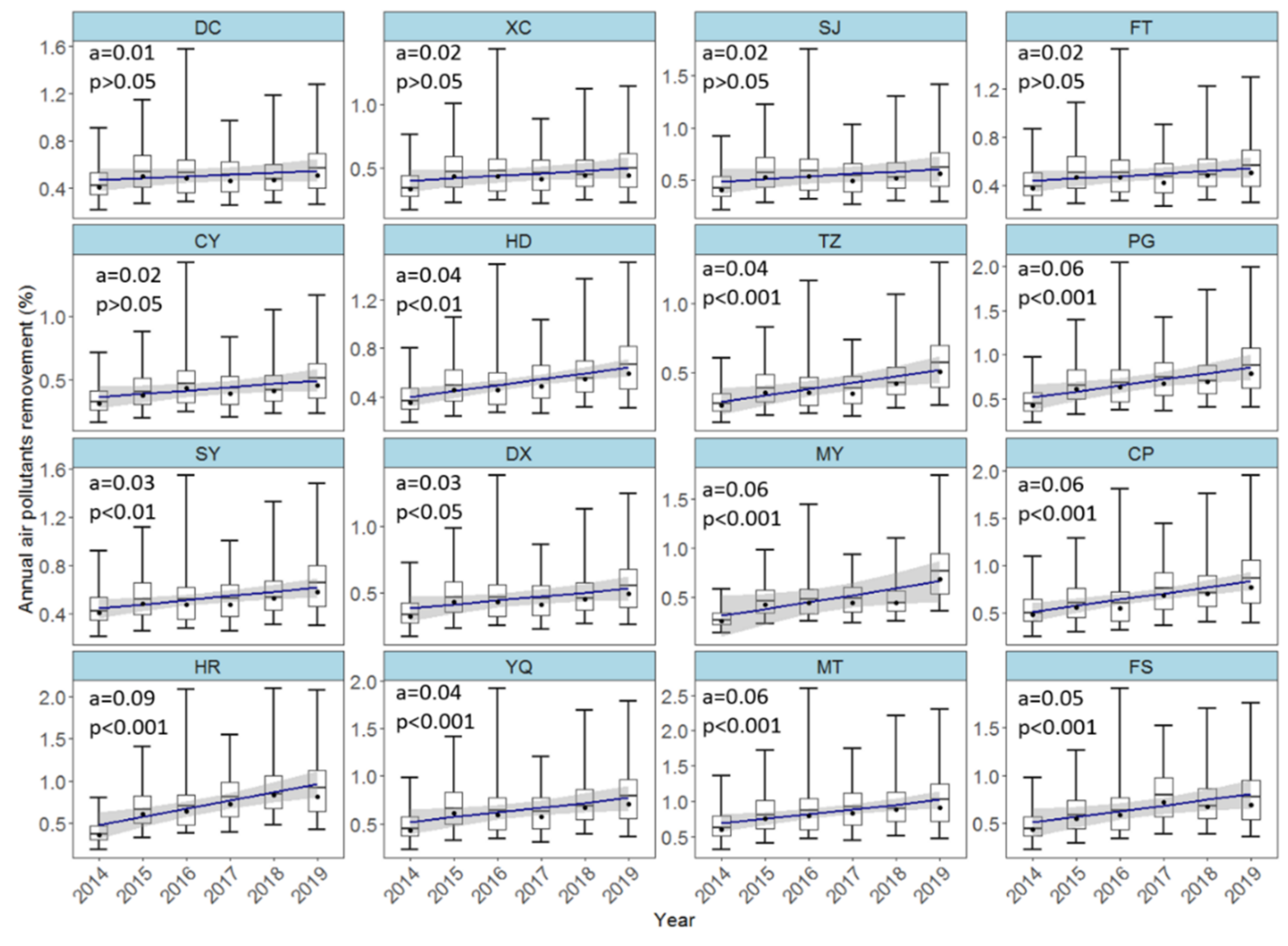
Figure 6 shows the proportion of atmospheric NO₂ removed by urban forests in the 16 districts according to boundary-layer height data. The boundary-layer height in Beijing varied widely between 2014 and 2019, with a maximum of 950 meters and a minimum of 220 meters. Average annual boundary-layer height ranged from 541 to 560 m. In general, annual absorption of NO₂ by urban forests in each district accounts for 0.14–2.60% of the total atmospheric NO₂ of the year. The average proportion of NO₂ removed by urban forests in the six urban districts was 0.46%, while the average proportion of NO₂ removed by forests in the 10 suburban districts was 0.57%. The difference of removal proportion between urban and suburban districts was significant (Wilcoxon signed-rank test, p < 0.001). The Mengtougou District (MT) had the highest average annual NO₂ removal proportion of 0.79% (range: 0.32–2.6%), while the Tongzhou District (TZ) had the lowest annual removal proportion of 0.38% (range: 0.14–1.29%). We found an increasing trend in the NO₂ removal proportion in each district, the mean rate of increase in urban districts was 0.02%, while in suburban districts it was 0.05%. The increasing trend of NO₂ removal proportion in the six urban districts was significantly lower than in the 10 suburban districts (p < 0.001). The increasing rate of removal proportion in the Huairou District (HR) was highest among the 16 districts, reaching 0.09% per year, while the Dongcheng District (DC) had the lowest rate of increase (0.01% per year), and the trend was not significant (p > 0.05).

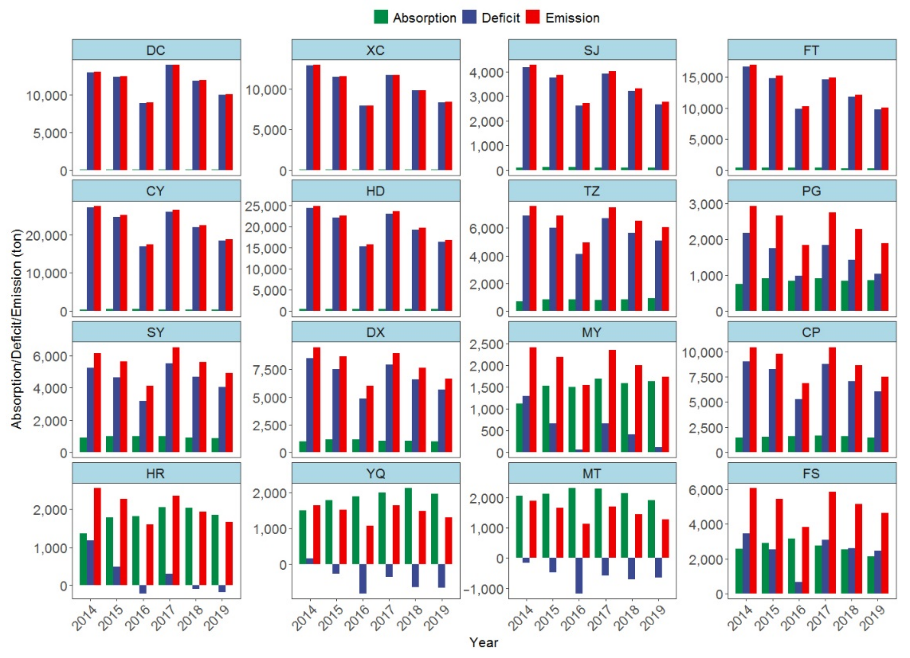
From the perspective of nitrogen neutrality, NO₂ emissions in the six urban districts are substantially higher than the amounts of NO₂ absorbed by urban forests (Figure 7). The supply of NO₂ absorption services provided by urban forests is largely insufficient compared with the emissions. In contrast, the supply of NO₂ absorption services in suburban forests is generally higher than in urban areas, and in some districts, the amount of NO₂ absorbed is higher than emissions. There is a huge difference between absorption and emission of NO₂ in Beijing, and total emissions are greater than absorption in most districts. The purification deficit between absorption and emission of NO₂ in the Chaoyang District (CY) was the largest among the 16 districts, with an average emission of 22,939 tons and average absorption of 460 tons in the period of 2014–2019, yielding a deficit of 22,479 tons. The Mentougou District (MT) and the Yanqing District were the only two districts where NO₂ absorption exceeded NO₂ emissions. For the Mentougou District, average annual emission was 1511 tons, and the average annual absorption was 2136 tons, exceeding emissions by 625 tons. For the Yanqing District, the average annual absorption was 1883 tons, and emission was 1447 tons, with absorption exceeding emissions by 436 tons.

4. Discussion

4.1. Spatial Distribution Pattern of NO₂ Absorption by Urban Forests in 16 Districts

The uneven distribution pattern of NO₂ absorption between urban areas and suburban areas may be influenced by the large differences in population density, building density, forest cover, and the quality of urban forests between the different districts in Beijing [23,28,29]. According to the deposition flux model (Equation (1)) and the total absorption amount model (Equation (6)), it can be inferred that the total absorption of NO₂ by urban forests has a positive linear relationship with atmospheric NO₂ concentration and the effective leaf area of urban forests, while the absorption per unit of green cover is mainly related to the local air pollutant concentration. In general, higher pollution concentrations, green land cover, and LAI lead to more pollutants absorbed by the vegetation, and this positive relationship has been found in many studies related to urban forests’ effects on air pollution removal [13,35,44]. The six urban districts are located in the central area of Beijing, which has a high population density and high fragmentation of urban forests that are mainly located in urban parks [45,46]. According to Yang, McBride, Zhou, and Sun [23], the vegetation in the green area of six urban districts is mostly pruned to maintain aesthetics, and overall effective leaf area is low despite some urban parks forming a large greenbelt. In contrast, the 10 districts located on the outskirts of the city are less densely populated and less densely built up, and the suburban area represented by the Mengtougou District, Miyun District, and Daxing District have large areas of forests [47]. These green areas are dominated by secondary forests with good growth conditions. The LAI of these forests is higher than in forests in urban areas [48]. The large difference in total leaf area between urban forests in urban and suburban areas is probably an important explanation for the differences in total absorption amount among different districts. According to the multiple regression analysis, the explanatory factor that most explains the urban–suburban differences in NO₂ absorption are population (42%) > economy (28%) > environment (20%) > energy consumption (10%) (Figure 3). A PCA analysis suggested that the characteristics of NO₂ absorption patterns of the 16 districts can be described by two principal components axes, respectively, economic–energy gradient variation and population-density–environmental gradient variation. On these two principal component axes, the six urban districts are mainly clustered in the areas with high population density and high per capita income but low NO₂ purification capacity, while the 10 suburban districts are clustered in the areas with lower population density and lower per capital income but higher NO₂ purification capacity (Figure 4). The gradient variation of purification capacity and population density reflects the imbalance in the distribution of air pollutant purification services supplied by urban forests in Beijing. A similar spatial pattern of air purification services characterized by “low center–high periphery” features was observed in studies conducted in centralized development cities [11,16,49].

4.2. Contribution of Urban Forests to Air Quality Improvement

The total NO₂ absorption capacity of urban forests in the 16 districts of Beijing from 2014 to 2019 is 14,910–17,747 tons, including 1338–1607 tons in the six urban districts and 13,438–16,235 tons in the 10 suburban districts. Our calculation of pollution removal in six urban districts in 2019 indicates the total absorption of NO₂ to be 1338 tons, which is comparable to the 1304 tons of NO₂ absorption found in a previous study conducted with a stable isotopic method in the same region [50]. Our results indicate that the annual NO₂ removal rate by urban forests in Beijing city is 0.5–1.6 g/m² for an annual NO₂ concentration within 22.0–66.9 µg/m³ in the 2014–2019 period. Our results compare well with the NO₂ removal rate of 0.5–2.8 g/m₃ by urban forests in Chile, with an annual NO₂ concentration of 48–190 µg/m³ [16]. The average annual absorption of NO₂ by urban forests in each district can neutralize 0.14–2.60% of the atmospheric NO₂ load, which can theoretically improve the air quality by 0.14–2.53% on average based on equation 11. The concentration of atmospheric NO₂ can be reduced by 0.10–0.34 µg/m³ due to the absorption by forests, which compares well with several studies conducted in urban areas [19,21]. The contribution of urban forests to atmospheric NO₂ mitigation under the current forest configuration is, however, not sufficient, and additional measures are currently applied in Beijing to control N pollution. These measures include the control of private car ownership, which significantly decreased domestic emission intensity per capita in the past decade [51]. Our findings address the potential NO₂ removal by trees in terms of atmospheric pollution mitigation, highlighting the role of urban forests as an important green infrastructure providing air purification services. Our results indicate that the urban forests in Beijing absorbed 9.90–15.80% of total NO₂ emissions during the period of 2014–2019, contributing to “nitrogen neutralization”, which is similar to the concept of “carbon neutralization” relying on plant CO₂ absorption. However, the effects of “nitrogen neutralization” are unbalanced between urban and suburban districts, with an overall neutralization ratio in the six urban districts ranging from 1.00 to 1.70%, compared with 11.20 to 14.00% in the suburban districts. This unbalanced pattern suggests that the current configuration of urban forests in Beijing may not be optimally configured for “nitrogen neutralization”.

4.3. Uncertainties and Limitations

In this study, local data for environmental factors (NO₂ concentrations and meteorological conditions) and ecological factors (LAI and deposition velocity) were adopted to ensure the accuracies of the i-Tree Eco deposition model in Beijing. The model estimations compared well with field measurements from a previous study [50]. However, some limitations are still inevitable due to the inherent uncertainties of the i-Tree Eco deposition model and the lack of time series for spatial data. The LAI of the 16 districts before 2019 was estimated based on the LAI product (30 m × 30 m) in 2019 combined with annual forest coverage data. More high-resolution and uniform LAI products should be adopted to improve the spatial resolution of plant NO₂ absorption in future studies. Another factor of uncertainty is the spatial heterogeneity of deposition velocity, which is influenced by local meteorological conditions and forest types [52,53]. This affects the accuracies of the i-Tree Eco model based on the multi-layer deposition model framework [34]. In our study, we calculated the annual average deposition velocity for different forest types based on the proportion of coniferous and broadleaf forests, which may cause uncertainties in the spatial heterogeneity of deposition velocity at fine scales. The spatial distribution of vegetation types based on more field surveys should be considered in future studies to improve the accuracy of deposition velocity.

Besides, the spatial interpolation method was used to obtain the spatial distribution of NO₂ concentration in the 16 districts of Beijing due to fewer monitoring stations located in the suburban areas than those in urban areas, which may result in higher estimated NO₂ concentration in the suburban districts, and therefore overestimation of NO₂ uptake capacity of suburban forests. Furthermore, more scenarios analysis combined with benefit analysis of different forest planting should be included in future studies.

4.4. Suggestions for Urban Forests Management

In this study, we estimated the potential NO₂ absorption by urban forests in Beijing during the period of 2014–2019 based on the i-Tree Eco deposition model, and some results from this study could serve as reference for urban green space planning and air pollution mitigation towards an “N-friendly society” for Beijing, from an “N source” stage to an “N neutrality stage” [22]. To achieve this goal, we propose the following:

• There is a significant imbalance in the distribution of NO₂ purification services by urban forests in Beijing. Although it is difficult to increase the area of urban forests in the central area of the city, the purification capacity of vegetation in urban forests can be improved by more natural management approaches, including reducing tree canopy pruning to increase the total leaf area of urban forests, and increasing the percentage of tree species with stronger NO₂ absorption used for roadside tree planting in urban areas, such as S. japonica [54]. The forest cover should be maintained in urban areas and expanded in suburban areas to contribute to Beijing’s capacity to achieve “carbon sequestration”, as well as advancing “nitrogen sequestration” [55,56].
• Urban forests can absorb atmospheric NO₂ and have a significant “nitrogen emission neutralization” effect. We found that urban forests can absorb 9.9–15.8% of total NO_x emissions, and in some districts, the absorption amount of NO₂ is higher than the total emissions. Plants can absorb NO₂ into their nitrogen pool to reduce the chance of NO₂ photolysis [8], thus reducing the potential of ozone precursor production [57], which are the emerging main air pollutants in most Chinese cities [58]. This suggests that near-ground ozone pollution can be addressed by enhancing NO₂ reduction and improving the “nitrogen emission neutralization” effect of urban forests.

5. Conclusions

The NO₂ absorption capacity of urban forests in the 16 districts of Beijing was assessed using the i-Tree Eco model. The total absorption of NO₂ by urban forests in the 16 districts was 14,910–17,747 tons in 2014–2019, and the removal rate per unit of green area was 0.5–1.6 g/m². The spatial pattern of NO₂ absorption is characterized by an imbalance of low absorption in urban centers and high absorption in suburban areas. The annual average absorption of NO₂ by urban forests in each district can account for 0.14–2.60% of annual total atmospheric NO₂ (ΔP_i(%)), which can improve the air quality by 0.14–2.53% (ΔC_i(%)) and reduce the NO₂ concentration by 0.10–0.34 µg/m³ (ΔC_i(µg/m³)) on average. Urban forests have a positive impact on reducing NO₂ concentrations, and the neutralization effect of NO_x emissions should not be ignored. Based on our estimation, 9.90–15.80% of NO₂ emissions can be absorbed by the forests in the 16 districts of Beijing. The overall neutralization ratio in the six urban districts ranged from 1.0 to 1.7%, while that of 10 suburban districts reached from 11.20 to 14.00%. The results of our study can provide suggestions for future urban forests planning and can also provide ideas for urban NO₂ mitigation based on a nature-based solution (NbS).

References

- Zhao, X.; Zhou, W.; Han, L. Human activities and urban air pollution in Chinese mega city: An insight of ozone weekend effect in Beijing. Phys. Chem. Earth 2019, 110, 109–116. [Google Scholar] [CrossRef]
- Gao, W.; Tie, X.; Xu, J.; Huang, R.; Mao, X.; Zhou, G.; Chang, L. Long-term trend of O-3 in a mega City (Shanghai), China: Characteristics, causes, and interactions with precursors. Sci. Total Environ. 2017, 603, 425–433. [Google Scholar] [CrossRef] [PubMed]
- Chan, C.K.; Yao, X. Air pollution in mega cities in China. Atmos. Environ. 2008, 42, 1–42. [Google Scholar] [CrossRef]
- Li, C.; Hammer, M.S.; Zheng, B.; Cohen, R.C. Accelerated reduction of air pollutants in China, 2017–2020. Sci. Total Environ. 2022, 803, 150011. [Google Scholar] [CrossRef] [PubMed]
- Wang, G.; Deng, J.; Zhang, Y.; Zhang, Q.; Duan, L.; Jiang, J.; Hao, J. Air pollutant emissions from coal-fired power plants in China over the past two decades. Sci. Total Environ. 2020, 741, 140326. [Google Scholar] [CrossRef] [PubMed]
- Xu, M.; Sbihi, H.; Pan, X.; Brauer, M. Local variation of PM2.5 and NO2 concentrations within metropolitan Beijing. Atmos. Environ. 2019, 200, 254–263. [Google Scholar] [CrossRef]
- Calfapietra, C.; Fares, S.; Manes, F.; Morani, A.; Sgrigna, G.; Loreto, F. Role of Biogenic Volatile Organic Compounds (BVOC) emitted by urban trees on ozone concentration in cities: A review. Environ. Pollut. 2013, 183, 71–80. [Google Scholar] [CrossRef]
- Tan, Z.; Lu, K.; Dong, H.; Hu, M.; Li, X.; Liu, Y.; Lu, S.; Shao, M.; Su, R.; Wang, H.; et al. Explicit diagnosis of the local ozone production rate and the ozone-NOx-VOC sensitivities. Sci. Bull. 2018, 63, 1067–1076. [Google Scholar] [CrossRef] [Green Version]
- Kumar, P.; Druckman, A.; Gallagher, J.; Gatersleben, B.; Allison, S.; Eisenman, T.S.; Hoang, U.; Hama, S.; Tiwari, A.; Sharma, A.; et al. The nexus between air pollution, green infrastructure and human health. Environ. Int. 2019, 133, 105181. [Google Scholar] [CrossRef]
- Xu, L.; He, N.; Yu, G. Nitrogen storage in China’s terrestrial ecosystems. Sci. Total Environ. 2020, 709, 136201. [Google Scholar] [CrossRef]
- Baró, F.; Haase, D.; Gómez-Baggethun, E.; Frantzeskaki, N. Mismatches between ecosystem services supply and demand in urban areas: A quantitative assessment in five European cities. Ecol. Indic. 2015, 55, 146–158. [Google Scholar] [CrossRef] [Green Version]
- Song, C.; Lee, W.-K.; Choi, H.-A.; Kim, J.; Jeon, S.W.; Kim, J.S. Spatial assessment of ecosystem functions and services for air purification of forests in South Korea. Environ. Sci. Policy 2016, 63, 27–34. [Google Scholar] [CrossRef]
- Manes, F.; Marando, F.; Capotorti, G.; Blasi, C.; Salvatori, E.; Fusaro, L.; Ciancarella, L.; Mircea, M.; Marchetti, M.; Chirici, G.; et al. Regulating Ecosystem Services of forests in ten Italian Metropolitan Cities: Air quality improvement by PM10 and O3 removal. Ecol. Indic. 2016, 67, 425–440. [Google Scholar] [CrossRef]
- Delaria, E.R.; Place, B.K.; Liu, A.X.; Cohen, R.C. Laboratory measurements of stomatal NO2 deposition to native California trees and the role of forests in the NOx cycle. Atmos. Chem. Phys. 2020, 20, 14023–14041. [Google Scholar] [CrossRef]
- Chen, C.; Wang, Y.; Zhang, Y.; Liu, C.; Lun, X.; Mu, Y.; Zhang, C.; Liu, J. Characteristics and influence factors of NO2 exchange flux between the atmosphere and P. nigra. J. Environ. Sci. 2019, 84, 155–165. [Google Scholar] [CrossRef]
- Escobedo, F.J.; Nowak, D.J. Spatial heterogeneity and air pollution removal by an urban forest. Landsc. Urban Plan. 2009, 90, 102–110. [Google Scholar] [CrossRef]
- Guidolotti, G.; Salviato, M.; Calfapietra, C. Comparing estimates of EMEP MSC-W and UFORE models in air pollutant reduction by urban trees. Environ. Sci. Pollut. Res. 2016, 23, 19541–19550. [Google Scholar] [CrossRef]
- Currie, B.A.; Bass, B. Estimates of air pollution mitigation with green plants and green roofs using the UFORE model. Urban Ecosyst. 2008, 11, 409–422. [Google Scholar] [CrossRef]
- Nowak, D.J.; Crane, D.E.; Stevens, J.C. Air pollution removal by urban trees and shrubs in the United States. Urban For. Urban Green. 2006, 4, 115–123. [Google Scholar] [CrossRef]
- Parsa, V.A.; Salehi, E.; Yavari, A.R.; van Bodegom, P.M. Analyzing temporal changes in urban forest structure and the effect on air quality improvement. Sustain. Cities Soc. 2019, 48, 101548. [Google Scholar] [CrossRef]
- Hirabayashi, S.; Nowak, D.J. Comprehensive national database of tree effects on air quality and human health in the United States. Environ. Pollut. 2016, 215, 48–57. [Google Scholar] [CrossRef] [PubMed]
- Xian, C.; Ouyang, Z.; Lu, F.; Xiao, Y.; Li, Y. Quantitative evaluation of reactive nitrogen emissions with urbanization: A case study in Beijing megacity, China. Environ. Sci. Pollut. Res. 2016, 23, 17689–17701. [Google Scholar] [CrossRef] [PubMed]
- Yang, J.; McBride, J.; Zhou, J.; Sun, Z. The urban forest in Beijing and its role in air pollution reduction. Urban For. Urban Green. 2005, 3, 65–78. [Google Scholar] [CrossRef]
- Beijing Municipal Ecology and Environment Bureau. Annual Report of Beijing Ecological Environment Statement in 2019; China Statistics Press: Beijing, China, 2019. [Google Scholar]
- Beijing Municipal Bureau Statistics. Beijing Statistical Yearbook; China Statistics Press: Beijing, China, 2020. [Google Scholar]
- National Bureau of Statistics of China. China Statistical Yearbook; China Statistics Press: Beijing, China, 2020. [Google Scholar]
- Zhang, Z.; Guan, H.; Xiao, H.; Liang, Y.; Zheng, N.; Luo, L.; Liu, C.; Fang, X.; Xiao, H. Oxidation and sources of atmospheric NOx during winter in Beijing based on δ18O-δ15N space of particulate nitrate. Environ. Pollut. 2021, 276, 116708. [Google Scholar] [CrossRef]
- Su, Y.; Gong, C.; Cui, B.; Guo, P.; Ouyang, Z.; Wang, X. Spatial Heterogeneity of Plant Diversity within and between Neighborhoods and Its Implications for a Plant Diversity Survey in Urban Areas. Forests 2021, 12, 416. [Google Scholar] [CrossRef]
- Su, Y.; Cui, B.; Luo, Y.; Wang, J.; Wang, X.; Ouyang, Z.; Wang, X. Leaf Functional Traits Vary in Urban Environments: Influences of Leaf Age, Land-Use Type, and Urban–Rural Gradient. Front. Ecol. Evol. 2021, 892, 681959. [Google Scholar] [CrossRef]
- Morani, A.; Nowak, D.; Hirabayashi, S.; Guidolotti, G.; Medori, M.; Muzzini, V.; Fares, S.; Mugnozza, G.S.; Calfapietra, C. Comparing i-Tree modeled ozone deposition with field measurements in a periurban Mediterranean forest. Environ. Pollut. 2014, 195, 202–209. [Google Scholar] [CrossRef]
- Emmerichs, T.; Kerkweg, A.; Ouwersloot, H.; Fares, S.; Mammarella, I.; Taraborrelli, D. A revised dry deposition scheme for land-atmosphere exchange of trace gases in ECHAM/MESSy v2.54. Geosci. Model Dev. 2021, 14, 495–519. [Google Scholar] [CrossRef]
- Zhang, L.; Brook, J.R.; Vet, R. A revised parameterization for gaseous dry deposition in air-quality models. Atmos. Chem. Phys. 2003, 3, 2067–2082. [Google Scholar] [CrossRef] [Green Version]
- De Jalon, S.G.; Burgess, P.J.; Yuste, J.C.; Moreno, G.; Graves, A.; Palma, J.H.N.; Crous-Duran, J.; Kay, S.; Chiabai, A. Dry deposition of air pollutants on trees at regional scale: A case study in the Basque Country. Agric. For. Meteorol. 2019, 278, 107648. [Google Scholar] [CrossRef]
- Zhang, L.M.; Moran, M.D.; Makar, P.A.; Brook, J.R.; Gong, S.L. Modelling gaseous dry deposition in AURAMS: A unified regional air-quality modelling system. Atmos. Environ. 2002, 36, 537–560. [Google Scholar] [CrossRef]
- Wu, J.; Wang, Y.; Qiu, S.; Peng, J. Using the modified i-Tree Eco model to quantify air pollution removal by urban vegetation. Sci. Total Environ. 2019, 688, 673–683. [Google Scholar] [CrossRef] [PubMed]
- Fang, K. Footprint family: Concept, classification, theoretical framework and integrated pattern. Acta Ecol. Sin. 2015, 35, 1647–1659. [Google Scholar]
- Feng, D.; Zhao, G. Footprint assessments on organic farming to improve ecological safety in the water source areas of the South-to-North Water Diversion project. J. Clean. Prod. 2020, 254, 120130. [Google Scholar] [CrossRef]
- Garcia-Palacios, P.; Gross, N.; Gaitan, J.; Maestre, F.T. Climate mediates the biodiversity-ecosystem stability relationship globally. Proc. Natl. Acad. Sci. USA 2018, 115, 8400–8405. [Google Scholar] [CrossRef] [PubMed] [Green Version]
- R Core Team. R: A Language and Environment for Statistical Computing; R Foundation for Statistical Computing: Vienna, Austria, 2020. [Google Scholar]
- Bartoń, K. MuMIn: Multi-Model Inference, R Package Version 1.10.5. 2014. Available online: https://r-forge.r-project.org/projects/mumin/ (accessed on 18 January 2022).
- Oksanen, J.; Blanchet, F.G.; Friendly, M.; Kindt, R.; Legendre, P.; McGlinn, D.; Minchin, P.R.; O’Hara, R.B.; Simpson, G.L.; Solymos, P.; et al. Vegan: Community Ecology Package. 2020. Available online: https://cran.ism.ac.jp/web/packages/vegan/vegan.pdf (accessed on 18 January 2022).
- Wickham, H. Ggplot2: Elegant Graphics for Data Analysis; Springer: New York, NY, USA, 2016. [Google Scholar]
- Tennekes, M. Tmap: Thematic Maps in R. J. Stat. Softw. 2018, 84, 1–39. [Google Scholar] [CrossRef] [Green Version]
- Cabaraban, M.T.I.; Kroll, C.N.; Hirabayashi, S.; Nowak, D.J. Modeling of air pollutant removal by dry deposition to urban trees using a WRF/CMAQ/i-Tree Eco coupled system. Environ. Pollut. 2013, 176, 123–133. [Google Scholar] [CrossRef]
- Qian, Y.G.; Zhou, W.Q.; Nytch, C.J.; Han, L.J.; Li, Z.Q. A new index to differentiate tree and grass based on high resolution image and object-based methods. Urban For. Urban Green. 2020, 53, 126661. [Google Scholar] [CrossRef]
- Li, F.; Zheng, W.; Wang, Y.; Liang, J.; Xie, S.; Guo, S.; Li, X.; Yu, C. Urban Green Space Fragmentation and Urbanization: A Spatiotemporal Perspective. Forests 2019, 10, 333. [Google Scholar] [CrossRef] [Green Version]
- Tang, H.; Liu, W.; Yun, W. Spatiotemporal Dynamics of Green Spaces in the Beijing-Tianjin-Hebei Region in the Past 20 Years. Sustainability 2018, 10, 2949. [Google Scholar] [CrossRef] [Green Version]
- Shi, Y.; Yang, G.; Feng, H.; Li, W.; Wang, R. Remote sensing of seasonal variability monitoring of forest LAI over mountain areas in Beijing. Trans. Chin. Soc. Agric. Eng. 2012, 28, 133–139. [Google Scholar]
- Bottalico, F.; Travaglini, D.; Chirici, G.; Garfì, V.; Giannetti, F.; De Marco, A.; Fares, S.; Marchetti, M.; Nocentini, S.; Paoletti, E.; et al. A spatially-explicit method to assess the dry deposition of air pollution by urban forests in the city of Florence, Italy. Urban For. Urban Green. 2017, 27, 221–234. [Google Scholar] [CrossRef]
- Gong, C.; Xian, C.; Cui, B.; He, G.; Wei, M.; Zhang, Z.; Ouyang, Z. Estimating NOx removal capacity of urban trees using stable isotope method: A case study of Beijing, China. Environ. Pollut. 2021, 290, 118004. [Google Scholar] [CrossRef] [PubMed]
- Xian, C.; Zhang, X.; Zhang, J.; Fan, Y.; Zheng, H.; Salzman, J.; Ouyang, Z. Recent patterns of anthropogenic reactive nitrogen emissions with urbanization in China: Dynamics, major problems, and potential solutions. Sci. Total Environ. 2019, 656, 1071–1081. [Google Scholar] [CrossRef]
- Wesely, M.L.; Hicks, B.B. A review of the current status of knowledge on dry deposition. Atmos. Environ. 2000, 34, 2261–2282. [Google Scholar] [CrossRef]
- Lin, J.; Kroll, C.N.; Nowak, D.J.; Greenfield, E.J. A review of urban forest modeling: Implications for management and future research. Urban For. Urban Green. 2019, 43, 126366. [Google Scholar] [CrossRef]
- Gong, C.; Xian, C.; Su, Y.; Ouyang, Z. Estimating the nitrogen source apportionment of Sophora japonica in roadside green spaces using stable isotope. Sci. Total Environ. 2019, 689, 1348–1357. [Google Scholar] [CrossRef]
- Liao, L.; Zhao, C.; Li, X.; Qin, J. Towards low carbon development: The role of forest city constructions in China. Ecol. Indic. 2021, 131, 108199. [Google Scholar] [CrossRef]
- Speak, A.; Escobedo, F.J.; Russo, A.; Zerbe, S. Total urban tree carbon storage and waste management emissions estimated using a combination of LiDAR, field measurements and an end-of-life wood approach. J. Clean. Prod. 2020, 256, 120420. [Google Scholar] [CrossRef]
- Prendez, M.; Carvajal, V.; Corada, K.; Morales, J.; Alarcon, F.; Peralta, H. Biogenic volatile organic compounds from the urban forest of the Metropolitan Region, Chile. Environ. Pollut. 2013, 183, 143–150. [Google Scholar] [CrossRef]
- Lu, X.; Zhang, L.; Chen, Y.; Zhou, M.; Zheng, B.; Li, K.; Liu, Y.; Lin, J.; Fu, T.-M.; Zhang, Q. Exploring 2016–2017 surface ozone pollution over China: Source contributions and meteorological influences. Atmos. Chem. Phys. 2019, 19, 8339–8361. [Google Scholar] [CrossRef] [Green Version]
Figure 1.
Landscape of Beijing city and administrative districts.
Figure 2.
Trend of NO2 absorption by urban forests in 16 districts of Beijing from 2014 to 2019. Mean absorption values are represented by points, max/min absorption is represented by error bars. The regression line was calculated based on the mean values. The 95% confidence interval of fitted mean value is represented by the shaded area.
Figure 3.
Annual total NO2 absorption and absorption of NO2 per unit of green area in 16 districts from 2014 to 2014. (A): annual total absorption in 10 suburban districts. (B): annual total absorption in six urban districts. (C): absorption of NO2 per green area in 10 suburban districts and range. (D): absorption of NO2 per unit of green area in six suburban districts and range. We tested the differences of mean total absorption in subgraph (A) and subgraph (B). For simplicity of the figure, only comparisons that are not significantly different are shown.
Figure 4.
Coefficients and relative effects of parameters of the multiple regression model (N = 96). Left subgraph: relative importance of parameters and adjusted R2 of the model. Right subgraph: average model coefficients based on the selection of AICc and max VIF. Mean coefficients and their 95% confidence interval are shown by points and error bars. The marks of significance are: ***: p < 0.001, **: p < 0.01, *: p < 0.05. Abbreviations: environmental factors: sulfur dioxide concentration (SO2), fine particulate matter concentration (PM); economic factors: industrial production value (GDP-I), GDP of construction, total retail sales of consumer goods (TVSRC), and per capita disposable income (PCDI); environmental protection expenditure (log(Exp-Env), log-transformed); energy consumption factor: total energy consumption (TEC); population factor: population density (POP-Den).
Figure 5.
Biplot of PCA analysis. Annual NO2 absorptions by urban forests of 16 districts are represented by points. Explanatory factor and absorption amount are represented by black and red arrows. The dashed circle is the equilibrium contribution circle, which is used to reflect the average contribution of all explanatory factors on the two principal component axes. Clustering results are represented by the light blue and light red 95% confidence circles.
Figure 6.
Annual removal proportion of atmospheric NO2 in the 16 districts of Beijing. The boxplots represent the range of removal proportion. Annual average removal proportions are represented by dots. Linear regressions were performed on the annual average removal proportion and year.
Figure 7.
Annual NO2 absorption, deficit, and emission in 16 districts. (Green bars: average annual NO2 absorption. Red bars: annual NO2 emission. Blue bar: purification deficit).
Publisher’s Note: MDPI stays neutral with regard to jurisdictional claims in published maps and institutional affiliations. |
© 2022 by the authors. Licensee MDPI, Basel, Switzerland. This article is an open access article distributed under the terms and conditions of the Creative Commons Attribution (CC BY) license (https://creativecommons.org/licenses/by/4.0/).
Share and Cite
MDPI and ACS Style
Gong, C.; Xian, C.; Ouyang, Z. Assessment of NO2 Purification by Urban Forests Based on the i-Tree Eco Model: Case Study in Beijing, China. Forests 2022, 13, 369. https://0-doi-org.brum.beds.ac.uk/10.3390/f13030369
AMA Style
Gong C, Xian C, Ouyang Z. Assessment of NO2 Purification by Urban Forests Based on the i-Tree Eco Model: Case Study in Beijing, China. Forests. 2022; 13(3):369. https://0-doi-org.brum.beds.ac.uk/10.3390/f13030369
Chicago/Turabian StyleGong, Cheng, Chaofan Xian, and Zhiyun Ouyang. 2022. "Assessment of NO2 Purification by Urban Forests Based on the i-Tree Eco Model: Case Study in Beijing, China" Forests 13, no. 3: 369. https://0-doi-org.brum.beds.ac.uk/10.3390/f13030369
Note that from the first issue of 2016, this journal uses article numbers instead of page numbers. See further details here.