Article

Estimating the Annual Above-Ground Biomass Production of Various Species on Sites in Sweden on the Basis of Individual Climate and Productivity Values

1
Department of Forestry and Wood Technology, Linnæus University, SE-351 95 Växjö, Sweden
2
Wood Science and Engineering, Wood Technology, SE-931 87 Skellefteå, Sweden
*
Author to whom correspondence should be addressed.
Forests 2014, 5(10), 2521-2541; https://0-doi-org.brum.beds.ac.uk/10.3390/f5102521
Submission received: 9 July 2014 / Revised: 6 October 2014 / Accepted: 20 October 2014 / Published: 22 October 2014

Abstract

:
The literature contains a large number of bioclimate, climate and biometric models for estimating the production of different species or stands under specific conditions on a defined site or models giving the distribution of a single species. Depending on the model used, the amount of input data required varies considerably and often involves a large investment in time and money. The purpose of this study was to create a model to estimate the annual above-ground biomass production of various species from site conditions defined by mean annual temperature and mean annual precipitation. For this approach, the Miami model of Lieth was used as a base model with some modifications. This first version of the modified model was restricted to sites in Sweden, where changes in the soil and groundwater level were relatively small, and where the growth of land vegetation was mostly dependent on temperature. A validation of this model has shown that it seems possible to use the Miami model to estimate the annual above-ground biomass production of various species, and that it was possible to compare the annual above-ground biomass production of different species on one site, as well as the annual above-ground biomass production of different species on different sites using the modeled data.

1. Introduction

The growth and geographical distribution of species are influenced by both abiotic and biotic factors. Abiotic factors for plants, also known as physical and chemical factors, are light, climate and geology [1,2]. Biotic factors are the effects of living organisms on the environment, such as the competition for resources and space, or natural enemies [3]. It is clear that no single factor affects the survival, development and fitness of plants, but that there is an optimum for each factor where plants grow best [4]. An increased distance from the optimum leads to greater stress, until the limit of tolerance is reached and death occurs. As there is no single optimum, but rather a number of different optima for different factors such as temperature, light, moisture, nutrients, etc., and as they are all available to different extents, there is always at least one factor that limits the growth; the one that is least available. This is in essence “the law of limiting factors”, first presented by Justus von Liebig in 1840 to explain the influence of chemical nutrients on plant growth. This approach can also be used to explain the existence of different ecosystems in different regions due to different climates [2]. The concept that the distribution of a species in any given region depends on the ecological niches available was introduced by Ellenberg, 1986, who designed ecograms for the tree species of Europe according to environmental factors [5,6].
The distribution of a species can be defined by abiotic factors, such as climate and substrate [7,8,9,10], and these factors were also used in models for the potential distribution of species. These models can be designed by a mechanistic or empirical approach as envelope models, climate response surfaces, homoclines, ecological niche models or species distribution models. Mechanistic models use critical climatic values for the physiological tolerance of different species to explain the range of distribution of the species. This means that a model for the distribution of a species is based on the critical physiological values measured in laboratory tests. In empirical models, climatic conditions are measured in the field together with the probability of occurrence of different species. These models result in a distribution pattern of the species and make it possible to predict the distribution under diverse climate scenarios. In contrast to mechanistic models, empirical models also show the biotic influences on the species [11]. An example of a mechanistic model for Northern Europe was STASH, which simulated the biogeographical distribution of individual species on a regional scale for the specific case of lodgepole pine (Pinus contorta Dougl.) in Scandinavia using scenarios from the Hamburg ECHAM3 climate model [12]. This bioclimatic model for the potential distributions of tree species in northern Europe was first published in 1996 [13].
Bioclimatic models on a global scale were used for modeling the carbon cycle. Models estimating the global net primary production (NPP, the difference between the CO2 fixed in plant biomass and the CO2 lost to the atmosphere) in units of bound carbon per unit area per annum are, for example, the Miami model [14], the Schuur model [15] and the National Center for Ecological Analysis and Synthesis (NCEAS) model [16]. The difference between these models is that the Schuur model was based on an extended data-set available for tropical regions, which allowed a better estimation under tropical climatic conditions than the Miami model [15]. For the NCEAS model, datasets were available from the Ecosystem Model Data Intercomparison (EMDI) project, for both grass-dominated and tree-dominated landscapes. Thus it was possible to calculate correlations for both grass- and tree-dominated sites. Furthermore, besides the NPP, the above-ground NPP (ANPP) was estimated [16,17]. By comparing the coefficients of determination for the modeled and observed NPPs of the three models with each other, it was shown that the coefficient of the Miami model lies between the coefficients of the two other models [16]. Nevertheless, these models estimate the NPP and not the ABM (above-ground biomass production of a single species in terms of dry matter).
The NPP, which reflects the gross primary production (GPP) minus the atmospheric loss or respiration (R), can be split into above-ground NPP (ANPP) and below-ground NPP (BNPP). The NPP/GPP ratio is between 0.44 and 0.47, and the ratio ANPP/GPP about 0.29 [18,19], so that a combination of the two results in an ANPP/NPP ratio of 0.62 to 0.66. Furthermore, since a BNPP/NPP ratio of about 0.35 is known [18], it can be suggested that the ANPP/NPP ratio is one minus the BNPP/NPP ratio, which leads to an ANPP/NPP ratio of 0.65. These relations show that it should be possible to use a model developed to estimate the NPP as a basis for estimating the ABM.
When one of the NPP models introduced above is used to estimate the ABM, the limiting factors are climatic factors, particularly the mean annual temperature and the mean annual precipitation. This implies that soil conditions can reduce the growth rate and that fertilization supports an increase towards the maximum growth. This was demonstrated in Norway spruce (Picea abies Karst). The production of Norway spruce in northern Sweden increased by 300% and in southern Sweden by 100% when nutrition and water supply were no longer limiting factors [20]. This result impressively showed the impact of the soil, as well as the strong influence that nutrients have on plant production. For that reason and because of the relatively small differences and exceptions regarding soil conditions in Sweden [21,22], the soil was not considered in this study, and the focus was set on climatic factors. With regard to the climate, it is important to know which factors are considered and how the borders are defined. Temperature, for example, is a limiting factor not only during the growth season but also during the period of dormancy. Miscanthus spp. is a perennial C4 grass, which has a photosynthetic mechanism obviously better adapted to low temperatures than that of various other C4 plants [23]. Tests in Northern Europe showed, however, that especially in the first two years of cultivation, high losses are possible because of too low winter temperatures [24]. In this context, it can be assumed that climate is the limiting factor for distribution, while soil conditions have a strong impact on the growth rate.
Compared to models estimating the potential distribution of a species, the NPP models mentioned above for the production of all species on a site are defined only by the climate variables. A greater specification of a model for a single species has the advantage of providing a more detailed estimate of the productivity or distribution; but the disadvantage is that the model is valid for only one species. As these models are, in general, complex, the adaptation required for further species is quite extensive. In contrast, no method yet exists to transform a NPP model estimating the productivity over all species into a species-specific model estimating the ABM.

2. Objectives

The purpose of this work was to estimate and compare the potential above-ground biomass production of some selected species in terms of dry matter (ABM) on two specific sites in Sweden and to assess whether it is possible to transform a global NPP model—the Miami model—into a species-specific ABM model.

3. Materials and Methods

For modeling the productivity of a species based on climate, a combination of species-specific parameters and climatic factors must be used. The basis of this concept is to find a correlation between productivity and climatic factors and to transform this correlation into a mathematical function. For this work, the mathematical formulation of the Miami model was chosen as a basis; but, since the Miami model estimates NPP, some modifications had to be made. In addition to the transformation of NPP to above-ground biomass production in terms of dry matter (ABM) of a single species, these modifications include the effects of evapotranspiration (E) and species-specific climatic parameters (MATnat).

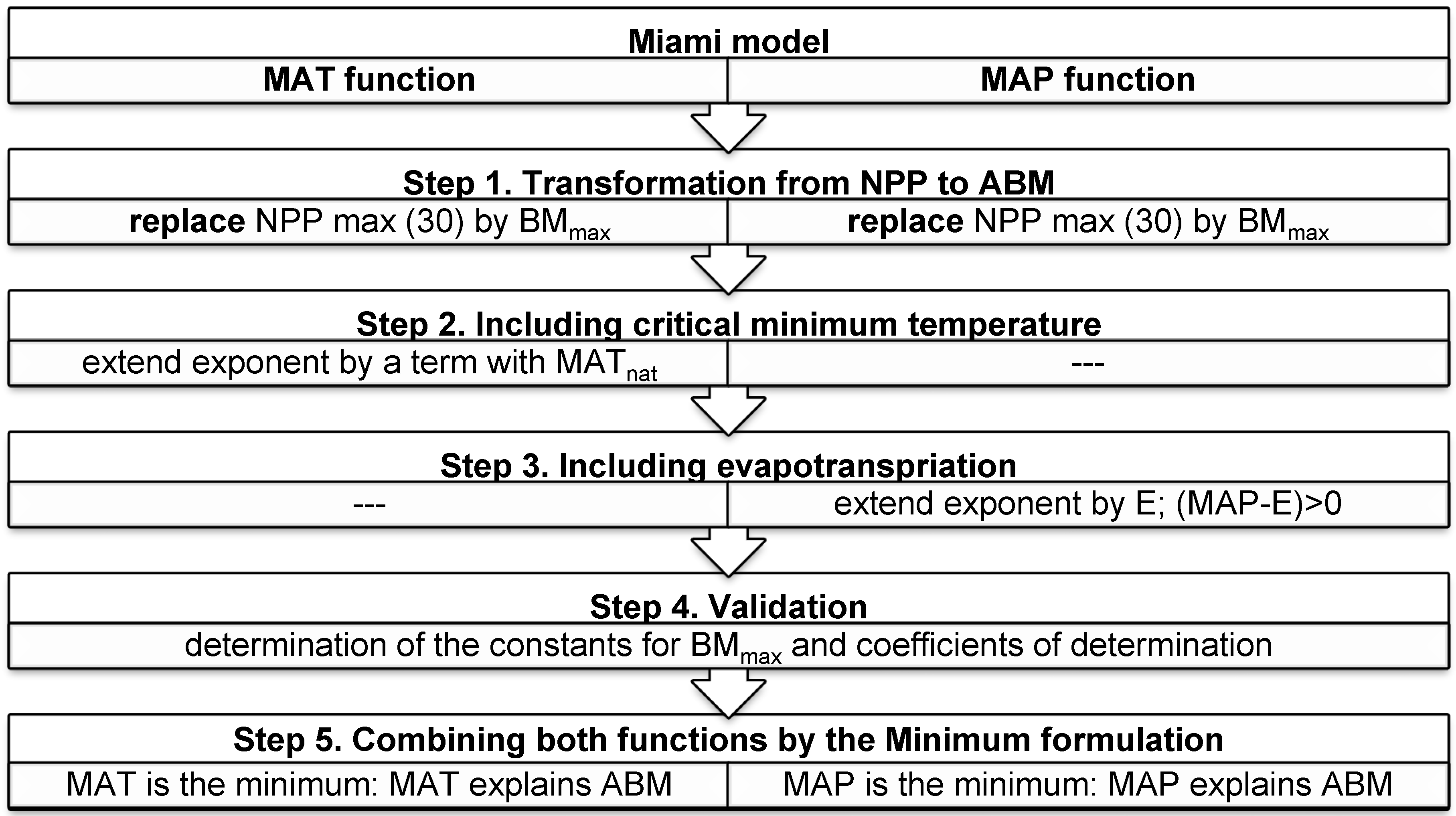
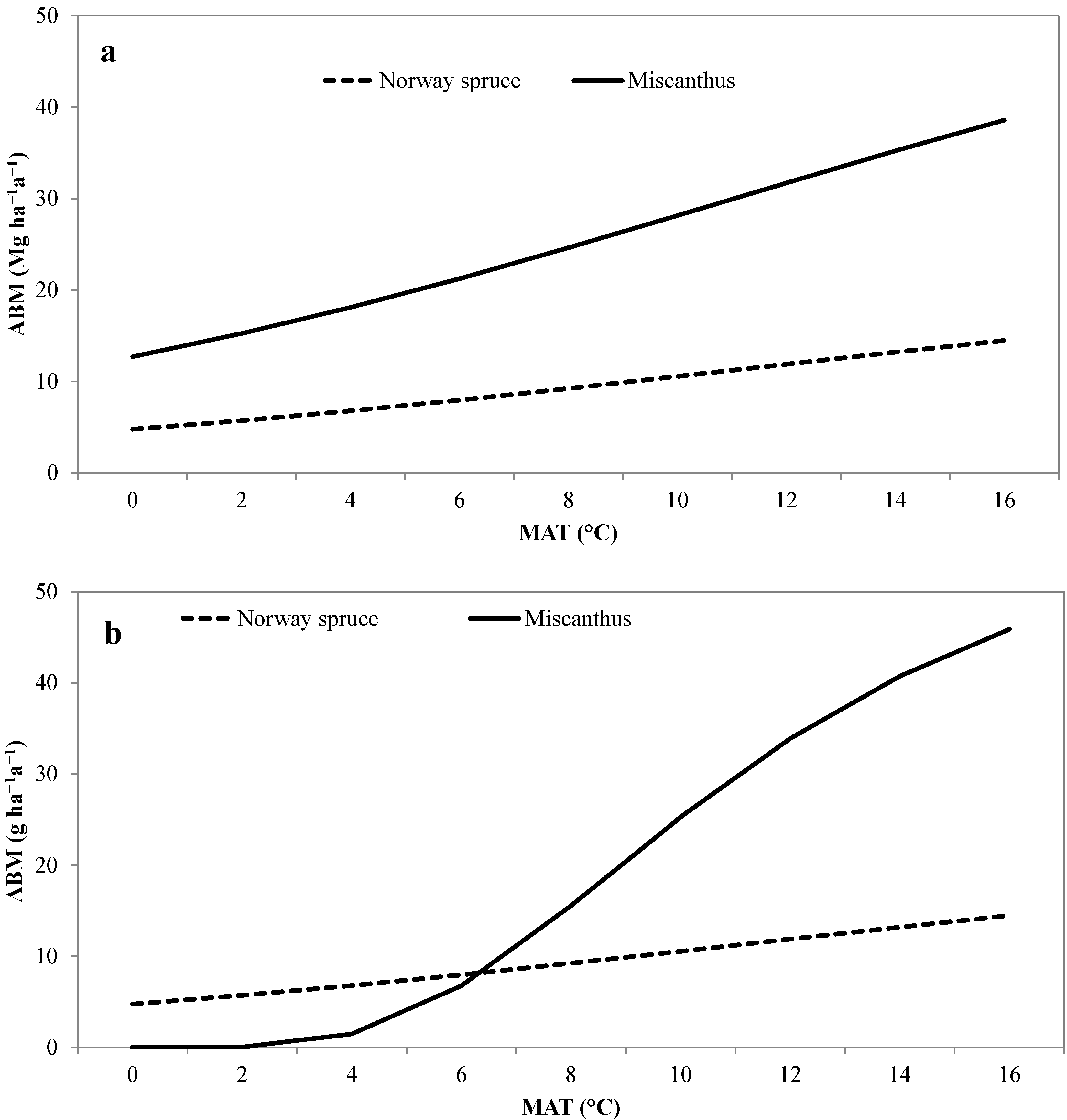
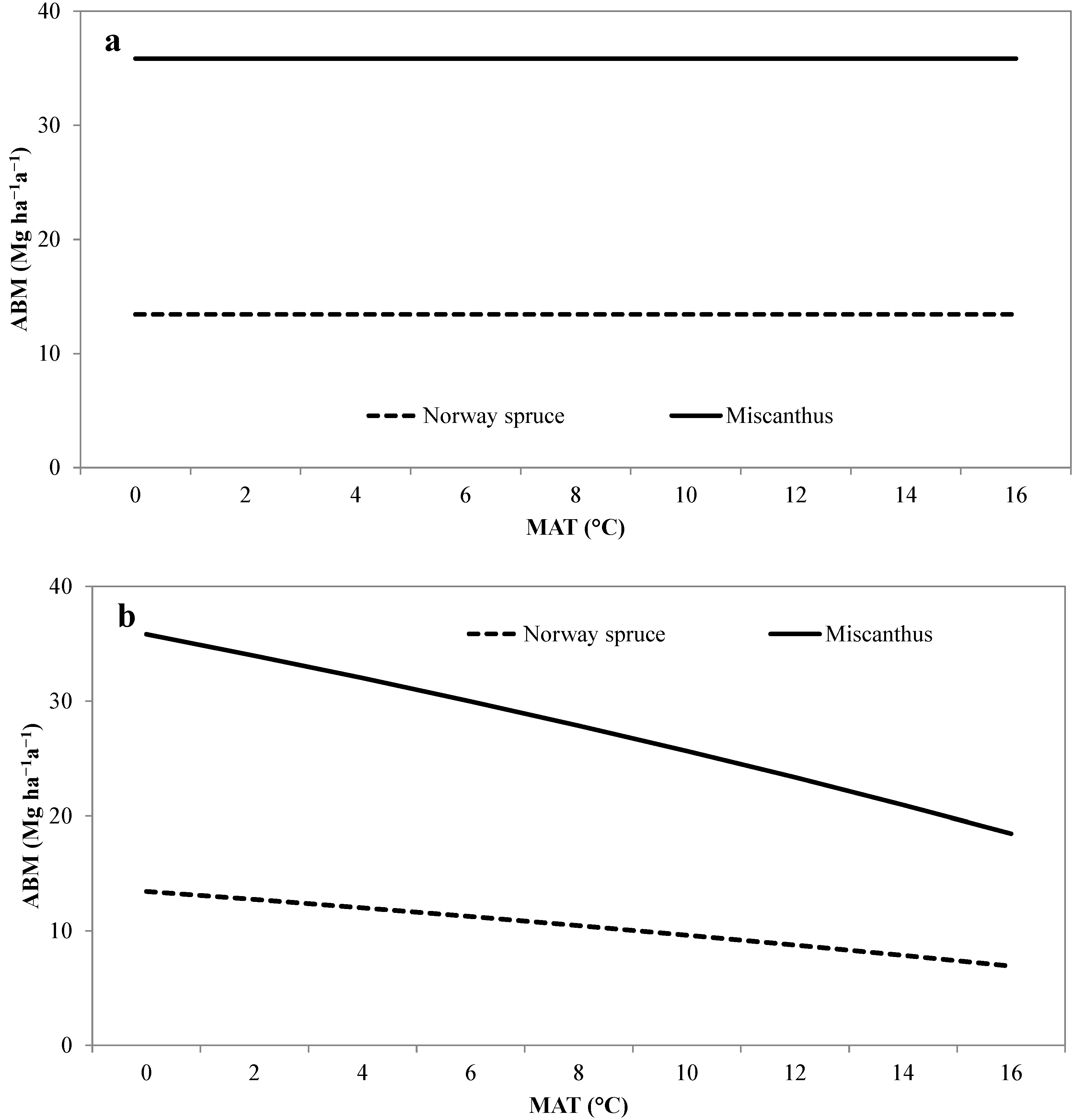
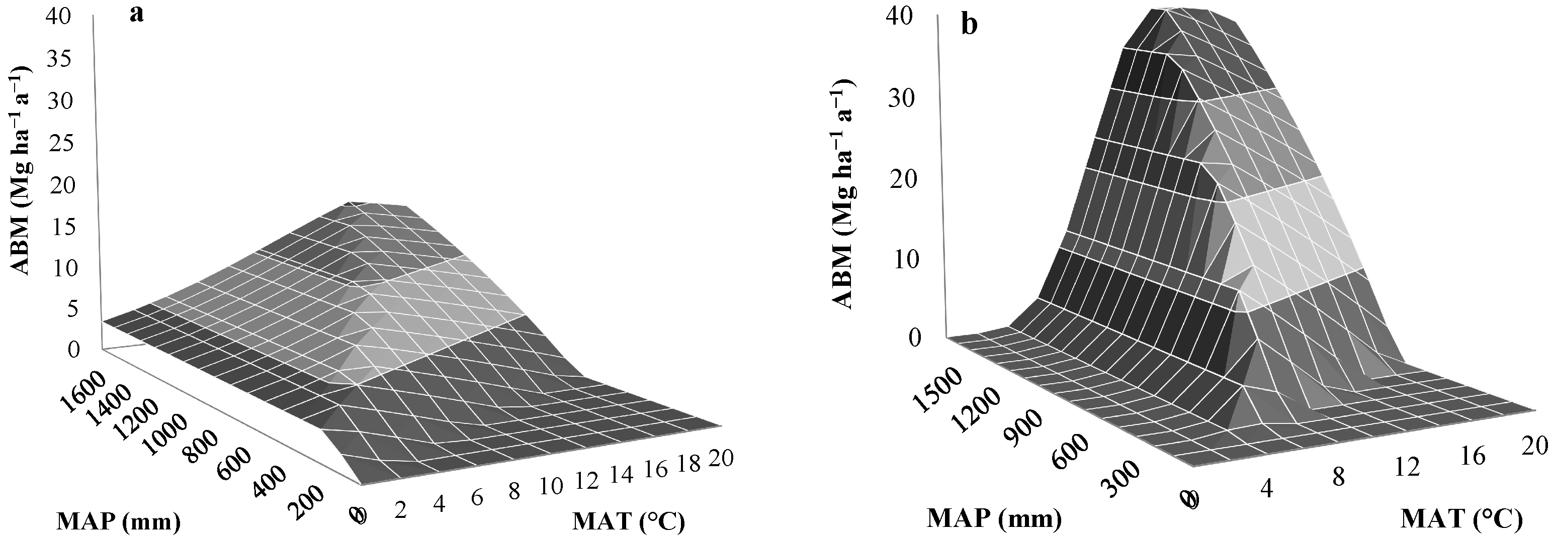
3.1. The Modified Miami Model

In the Miami model, the global net primary production (NPP) is estimated using the limiting productivity level defined either by the mean annual temperature in degrees centigrade (MAT) or the mean annual precipitation in millimeters (MAP). This means that NPP is expressed as:
NPPMAT = 30/(1 + e1.315 − 0.119MAT) (Mg ha−1a−1)
where MAT is the mean annual temperature (°C), or as:
NPPMAP = 30 × (1 − e−0.00066MAP) (Mg ha−1a−1)
where MAP is the mean annual precipitation (mm). Each lower value of NPP is estimated from the two functions:
NPP = Min(NPPMAT; NPPMAP) (Mg ha−1a−1)
Equations 1 and 2 are non-linear functions with a maximum productivity of 30 tons per hectare per year [14]. It is suggested that the NPP model can be transformed into a species-specific model by including two species-specific variables, the “maximum above-ground biomass production in the dry matter of a species” (BMmax) and the “MAT of the native distribution area of a species” (MATnat). Figure 1 gives an overview of the transformation of the Miami model. Moreover, it is supposed that evapotranspiration is linearly related to MAT [25].
The formulations of the two functions of the Miami model (Equations 1 and 2) support this type of modification. The exposed maxima of the two functions can be replaced by the BMmax found in the literature. As the Miami model was not designed for a single species, but for the collectivity of species on a single site, the MBmax has to be multiplied by a constant to avoid systematic underestimation of the biomass production of a single species. This constant is found by approximation of the modeled data to the literature data. Approximation during the validation process showed that for the above-ground biomass production of a species in the dry matter (ABM) modeled by the MAT, multiplication of the BMmax by 1.5 (Equation 4) and for the ABM modeled by the MAP a multiplication of the MBmax by 2 (Equation 5) offer the best estimations by the model. The different BMmax potentials of single species leads to a fan of graphs differing only by a constant expressed by the differences in BMmax. This formulation is problematic for species with a high BMmax and adapted to warmer climates, such as Paulownia spp. [26,27]. Because of their weak frost resistance, such species can hardy survive under cooler conditions, and this leads to very low or no ABM at low MATs. This requirement can be fulfilled without changing the maximal values by extending the exponential MAT function (Equation 1) by MATnat within the exponent (Equation 4). The influence of MATnat expresses itself in an increasing gradient with an increase in MATnat, resulting in a shift of the zero-point in the direction of the inflexion point of the graph (Figure 2). This means that a higher MATnat leads to the start of biomass production at a higher temperature. The exact formulation of the term for MATnat was found by approximation during the validation process.
Figure 1. Illustration of the modification of the Miami model in order to transform the net primary production (NPP) model into a species-specific ABM model. Modification of the MAT function is shown on the left and of the MAP function on the right. MAT, mean annual temperature (°C); MAP, mean annual precipitation (mm); NPP, global net primary production (Mg ha−1a−1); MATnat, mean annual temperature of the native distribution area of a species (°C); ABM, modeled above-ground biomass production of a species in dry matter (Mg ha−1a−1); BMmax, maximal above-ground biomass production in dry matter of a species found in the literature (Mg ha−1a−1); E, mean annual evapotranspiration (mm).
Forests 05 02521 g001
Figure 2. ABM modeled as a function of MAT using the MAT function and showing the influence of MATnat: (a) ABM of Norway spruce and Miscanthus without the influence of MATnat; (b) Norway spruce with a MATnat of 1°C and Miscanthus with a MATnat of 18 °C; ABM, modeled above-ground biomass production of a species in dry matter (Mg ha−1a−1); MAT mean annual temperature (°C); MATnat, mean annual temperature of the native distribution area of a species (°C).
Forests 05 02521 g002
Higher temperatures may not always result in higher biomass production, as the evapotranspiration increases with increasing temperature [28]. This suggests that the ABM at a constant MAP estimated by the MAP function (Equation 2) is not constant over MAT, but rather decreases (Figure 3).
Figure 3. ABM modeled as a function of MAT using the MAP function with MAP = 900 mm and showing the influence of E: (a) ABM of Norway spruce and Miscanthus without E; and (b) after including E in the MAP function. ABM, modeled above-ground biomass production of a species in dry matter (Mg ha−1a−1); MAT, mean annual temperature (°C); MAP, mean annual precipitation (mm); E, mean annual evapotranspiration (mm).
Forests 05 02521 g003
In addition, since the MAP equation is an exponential function, the mean annual evapotranspiration (E) has to be included in the exponent to achieve a change of gradient in the MAP graph (Equation 5). The linear function of E, as E represents the above-ground water loss compared to MAP as water input, suggests that the best formulation is to subtract E from MAP. A restriction in this formulation is that MAP minus E cannot be negative, as there is no negative biomass production. This restriction is solved by the logic formulation “if the term is negative, set it to zero”.
The final formulation of the modified Miami model is: the relationship between the modeled ABM and the MAT, including the MATnat for a single species on a specific site is given by:
ABMMAT = 1.5 × BMmax/(1 + e((MAT+MATnat)/(MAT + 1)) × (1.315 − 0.119MAT)) (Mg ha−1a−1)
In addition, the relationship between ABM and the MAP including the restriction that E ≤ MAP for a species on a specific site is given by:
ABMMAP = 2 × BMmax × (1 − e−0.00066(MAP − E)) (Mg ha−1a−1)
The relationship between E and the MAT is given by:
E = MAT × 31.4 (mm)
The relationship between ABM, MAP and MAT is given by:
ABM = Min (ABMMAT; ABMMAP) (Mg ha−1a−1)
Where BMmax is the maximum above-ground biomass production in the dry matter of a species (Mg ha−1a−1); MATnat is the mean annual temperature of the native distribution area of a species (°C); E is the mean annual evapotranspiration (mm); MAT is the mean annual temperature (°C); MAP is the mean annual precipitation (mm). Furthermore, the model has two restrictions regarding MAT that have to be considered:
(1)
MAT ≥ 0 °C: this model gives an estimate of ABM, starting at a MAT of 0 °C. It is not valid for values below 0 °C.
(2)
MATnat > 0 °C: the MATnat must be positive because of the mathematical formulation.

3.2. Validation of the Modified Miami Model

For approximation and validation of the model, four different species were chosen, two of them adapted to cool climates, Norway spruce and reed canary grass (Phalaris arundinacea L.), and two highly productive species with a low frost resistance, Paulownia spp. and Miscanthus spp. Typical MATnat values and very high BMmax values for the four species were found in the literature as input data for the model. The modeled data (ABM) were compared (r2) with the literature data (BMmax), and the result is presented in Table 1. The species-specific parameters were chosen as follows:
Norway spruce is a native species of taiga and montane forests, but cultivation has extended its area in Northern and Central Europe [29]. As the species is native to the boreal forest, a MATnat of 1 °C was suggested. The BMmax was chosen as 15 Mg ha−1a−1 in accordance with the findings of Bergh, Linderand Bergström [20].
Reed canary grass is native to nearly all of Europe, except above the Arctic Circle and some southern regions. The MATnat for reed canary grass was set at 2 °C, as it grows best under cool and moist conditions [30], and the BMmax was chosen as 14 Mg ha−1a−1 [31].
Paulownia is a species originating from Asia with an average MATnat of about 17 °C [26]. While some species within this genus show frost resistance at about −20°C, others tolerate no frost [27]. Estimations based on growing tests gave values of 35 to 90 Mg ha−1 in two to three years [32]. For this study, 36 Mg ha−1a−1 (90 divided by 2.5) was chosen as BMmax.
Miscanthus is a highly productive species native to Southeast Asia with a MATnat of about 18 °C [23,33]. Growth tests on Miscanthus showed that yields of more than 40 Mg ha−1a−1 could be achieved [34].
Table 1. Literature data, parameters and output of the final modified Miami model. MAT, mean annual temperature; MAP, mean annual precipitation; BMmax, maximal above-ground biomass production of a species in dry matter; MATnat, mean annual temperature of the native distribution area of a species; ABM, modeled above-ground biomass production of a species in dry matter; r2, coefficient of determination for the final model.
Literature dataParametersOutput
SpeciesMATMAPBMmaxBMmaxMATnatABMr2References
°CmmMg ha−1a−1Mg ha−1a−1°CMg ha−1a−1-
Norway spruce0.0718 *4.51514.80.90[20,35,36,37]
2.0718 *6.25.7
4.0718 *7.96.8
6.0718 *9.68.0
8.0718 *11.38.0
10.0718 *13.07.0
Reed canary grass4.66326.41426.00.58[31,38,39,40,41,42]
5.97506.27.0
6.96576.07.1
7.65145.54.7
8.24776.23.8
8.45476.24.8
Miscanthus7.678311.8401813.70.41[23,24,34,43,44]
7.857815.114.6
8.363014.717.0
8.963415.416.7
9.668918.518.1
9.676912.621.2
9.676617.521.1
9.866021.016.6
10.459419.612.9
10.459412.512.9
10.567619.616.3
11.581334.320.6
* Estimated mean values.
Comparison of the BMmax values from the literature with the modeled BMmax shows an underestimation of BMmax, especially at higher MAT. The reason is that the BMmax values from the literature are extremely high values, partly achieved in growing tests. These extreme values can be much higher than average values, because of regional and experimental variation in nutrients and water supply. The difference increases with increasing MAT, because the importance of water as a limiting factor is intensified. The inclusion of MAP and E in the model therefore leads to an underestimation of BMmax by the model compared to the literature data. In the case of Norway spruce, for example, the high BMmax values were achieved by fertilization and irrigation. As modeling was based on a MAP of 718 mm, the impact of the water-limitation increased with increasing MAT.
The values for the coefficient of determination (r2) in Table 1 are between 0.41 and 0.90. Nevertheless, the small amount and small range of data may reduce the representative significance of the coefficient of determination. Therefore, the coefficient of determination for the different species, the paired samples correlation (t-test), was also used to increase the parameters by combining all the literature data presented in Table 1 under a single variable and comparing them to modeled data. For this purpose, the species-specific parameters (MATnat and BMmax) were exchanged either (1) by using the literature data directly as species-specific parameters or (2) by using average variables over all species for the parameters.
(1)
The literature data were compared to modeled data using each single MATnat and BMmax value in the literature directly as a species-specific parameter. The coefficient of determination of this modification was r2 = 0.903 with p < 0.0001.
(2)
The literature data were compared to the modeled data using as parameters the average MATnat and BMmax values from the literature data. The coefficient of determination of this modification was r2 = 0.759 with p < 0.0001.
For the paired sample comparisons (1) and (2), it could not be excluded that the two groups (the literature data and the modeled data) were equal, and this supports the hypothesis that the modified Miami model can be used to estimate the ABM. Thus, the results of the paired sample comparisons support the results of the validation based on the approximation process (Table 1), i.e., that it is possible to estimate the ABM of a single species with the modified Miami model using species-specific variables.
To see the effect of the species-specific variables and the relation between the MAT (Equation 4) and MAP (Equation 5) functions (Equation 7), 3D graphs were drawn for Norway spruce and Miscanthus (Figure 4) using the species-specific parameters introduced above. The effect of the different BMmax and of the MATnat with a later start of biomass production in combination with a higher grade led to strong differences between the graphs for the two species.
Figure 4. ABM of (a) Norway spruce and (b) Miscanthus as functions of MAT and MAP; the species-specific parameters (BMmax, MATnat) result in different starts, different increases and, finally, in different amounts of ABM. ABM, modeled above-ground biomass production of a species in dry matter (Mg ha−1a−1); MAP, mean annual precipitation (mm); MAT, mean annual temperature (°C); BMmax, maximal above-ground biomass production in dry matter of a species in the literature (Mg ha−1a−1); MATnat, mean annual temperature of the native distribution area of a species (°C).
Forests 05 02521 g004

3.3. Choice of Species-Specific Parameters for the Modified MIAMI Model to Estimate the Above-Ground Biomass Production in Dry Matter for Different Selected Species

The modified Miami model was used to estimate the above-ground biomass production of a species in the dry matter (ABM) of different species on the two sites in Sweden. To compare the ABM of different species on different sites using the modified Miami model, the species-specific parameters for all the species and climate data for all the sites were needed. Table 2 shows the species-specific variables (BMmax and MATnat) in the literature for the different species. The climate data for the two sites are (1) for southern Sweden a MAT of 6 °C and MAP of 750 mm and (2) for northern Sweden a MAT of 3 °C and MAP of 601 mm. The site in northern Sweden lies in the fifth hardiness climate zone, and the site in southern Sweden in the seventh climate zone [45]. On both sites, three species, Norway spruce, Scots pine (Pinus sylvestris L.) and birch (Betula spp.), have together more than 90 percent of the standing volume of all land use classes [46]. In the region of the northern site, the total number of different tree species was 10. Of these, the most frequent was Scots pine with 43.1%vol. In the region of the southern site, sixteen species were found, the most frequent species being Norway spruce with 48.5%vol. The mean volume increment, including the growth of felled trees on forest land, was 3.0 and 5.7, respectively [46]. The soil on both sites is brown soil, and the dominant humus layers are duff and mull in the two regions. The regions are further characterized mainly by Podzols with high frequencies of clay [47]. For BMmax, the averages of the relatively higher biomass production values found in the literature were chosen. The MATnat values are either mean annual temperature values for the native region, when available, or averages of the mean annual temperature values from growing tests, plantations and forestry documented in the literature.
Table 2. Literature values of the maximum biomass production of a species in dry matter (BMmax) and the mean annual temperature of the native distribution area or the average mean annual temperature of the reported growing tests (MATnat) for different species.
SpeciesBMmaxMATnatReferences
Mg ha−1a−1°C
Picea abies Karst10.80.5[48,49,50,51,52,53]
Pinus sylvestris L.7.30.1[50,51,52,53,54,55]
Abies alba Mill.9.12.6[50,51,52,53,54,55,56,57]
Larix spp.9.13.9[50,51,52,58,59,60,61,62]
Pseudotsuga menziesii Mirb. Franco14.27.6[52,63,64,65,66]
Betula spp.6.70.3[50,51,53,55,67]
Alnus glutinosa (L.) Gaertn.7.72.7[51,53,68]
Populus nigra L.8.89.1[69,70,71,72,73,74,75]
Populus tremula L.8.81.9[50,53,67,71,76,77,78,79]
P. tremula L. x p. tremuloides Michx.11.41.0[71,76,80,81]
Salix spp. (short rotation)12.55.3[50,71,74,75,82,83]
Fraxinus excelsior L.8.79.6[51,55,75,84,85,86,87]
Fagus sylvatica L.10.09.5[51,52,55,73,84,85,86,87]
Quercus spp.7.49.9[51,52,73,75,84,85,86]
Tilia spp.8.39.4[84,88,89]
Acer platanoides L.7.09.9[51,75,84,85,87]
Paulownia spp.28.316.8[26,32,90,91]
Miscanthus spp.23.518.4[33,34,44,71,92,93]
Phalaris arundinacea L.10.52.0[31,41,42,94,95,96]

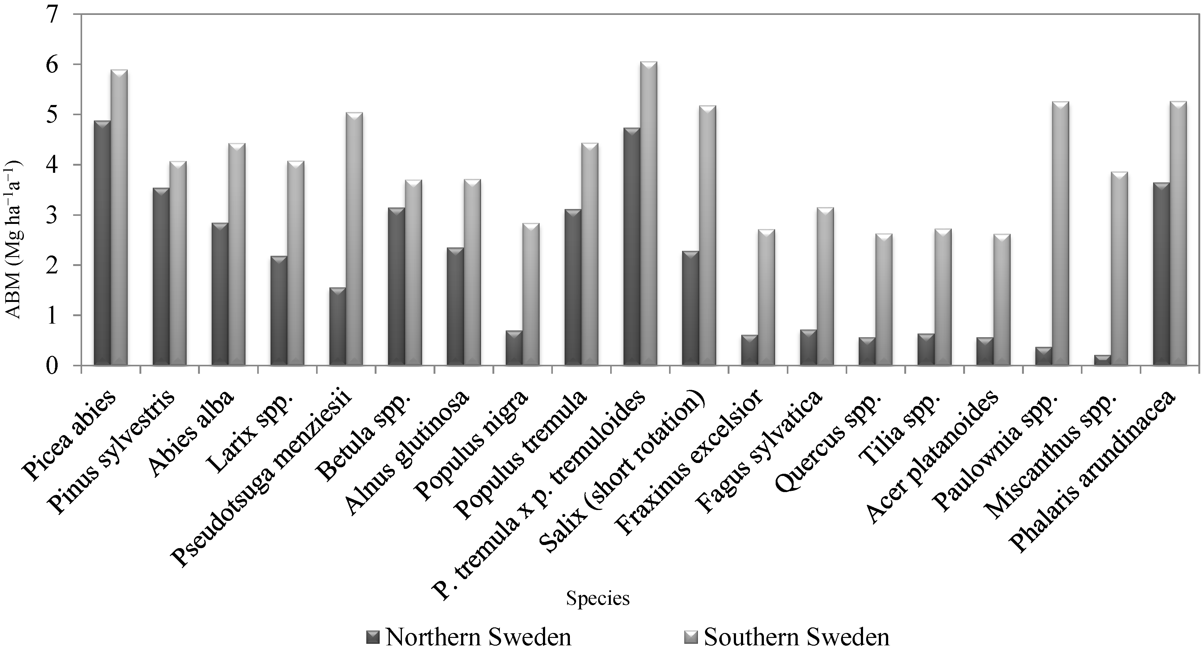
4. Results and Discussion

The species-specific variables presented in Table 2, together with the climate data for the two sites described above, were used as input parameters for the modified Miami model. Figure 5 shows the estimated above-ground biomass production of a species in dry matter (ABM) for the different species in both northern (black) and southern Sweden (grey). Although the absolute values for the different species may include a large variation in ABM for a single site, there is a clear trend in the differences between species at the two sites.
Figure 5. ABM of selected species for two sites in Sweden with a MAT of 3 °C and MAP of 601 mm (northern Sweden); and a MAT of 6 °C and MAP of 750 mm (southern Sweden); ABM, modeled above-ground biomass production of a species in dry matter (Mg ha−1a−1); MAT, mean annual temperature (°C); MAP, mean annual precipitation (mm).
Forests 05 02521 g005
Most of the species have ABM values in the range of 2 to 4 Mg ha−1a−1 for the site in southern Sweden (Figure 5 grey). Eight of the 19 species have an ABM between 4.5 and 6 Mg ha−1a−1. This is often less than half of the maximum biomass production presented in the literature (BMmax). The three species with the highest ABM are hybrid aspen (P. tremula L. × P. tremuloides Michx.), Norway spruce and reed canary grass.
In northern Sweden (Figure 5, black), the only species with a biomass production higher than 4 Mg ha−1a−1 are Norway spruce and hybrid aspen, while Scots pine, birch and aspen (Populus tremula L.) show a production of more than 3 Mg ha−1a−1. Reed canary grass also has a relatively high productivity, which explains why it is cultivated to such an extent in the boreal regions, a fact also supported by literature [38,40,95].
Of the broad-leaved trees, only the pioneer species, such as birch and aspen or alder (Alnus glutinosa (L.) Gaertn.), appear able to survive under boreal climatic conditions, which is also supported by forest inventory data [46]. The findings for other species are also supported by the literature: for Paulownia plantations, a MAT of at least 9 °C [97] or at least the sixth climate zone [98] are recommended, due to the low frost resistance of the fast growing variants of this species [26,27]; for Miscanthus, problems of cultivation in colder climate zones were reported [24]. Silver fir (Abies alba Mill.) and Douglas fir (Pseudotsuga menziesii (Mirb.) Franco) favour not overly cool climates with a relatively high precipitation [6,65,99,100]. For the species native to Sweden, the inventory data, such as the percentages of different species in the forest, support the results of the model [46].
The results, which include (1) a comparison of different species on one site and (2) a comparison of two different sites, show that it is possible to estimate the ABM for different species on different sites using the modified Miami model. This means that this model can be used as a decision support for the plantation of species under different climate conditions, because it shows that the extent of temperature or precipitation are limiting factors for biomass production. The results also demonstrate that both requirements, namely the variation in biomass production and the influence of the minimal temperature for the different species, can be fulfilled.
Nevertheless, it is only a basic formulation to be optimized and validated with a larger quantity of reference data. The most challenging task during the modeling and validation of the model was to find verified data. When data are found, they are generally presented in a more or less wide range, which gives a subjective perspective to the dataset used within the model, even if it was intended to be objective. Most critical for this concept is the use of MAT values from the native distribution area (MATnat) of a species. For some species, it is relatively easy to find plausible values, since they are well documented or native in a relatively limited area, but for others it is quite difficult and this means that mean values estimated over an extended area have to be used. Besides the inclusion of MATnat, the inclusion of evapotranspiration (E) in the MAP function is considered as critical. For this study, the linear correlation between MAT and E according to the findings of Komatsu, Maita and Otsuki [25] was used. However, since E was not allowed to exceed MAP, because this would result in negative biomass production, a logical function had to be included, setting any negative value to zero. Optimization might eliminate this problem. Furthermore, the model has not been verified for higher temperatures, where the MAP function becomes more important. According to the findings of Komatsu, Maita and Otsuki, verification in the range of higher temperatures will show whether it is possible to use the function of E originally developed for mountain forest areas in Japan or whether further adaptation is necessary. However, the best option would be a global formulation for the correlation between MAT and E.
If optimization is carried out for water availability, attempts should be made to manage this via the distribution of precipitation over the year rather than soil water capacity; this approach would further exclude soil data. In general, soil texture and soil structure are critical impact factors, for instance because of water storage capacity and nutrient supply. In Sweden, soil data are quite similar over the entire country, and the factor soil could therefore be treated as a constant in the present study, but this would not be valid for other regions in Europe. On the other hand, topography, even on a small scale, also has a very strong influence on water and nutrient supply, and this would make more general modeling on a larger scale impossible. Furthermore, the exclusion of soil as a separate parameter increases the importance of the choice of the BMmax parameter. Even if soil with poorer conditions would be a reduction factor for the biomass production of the species, this fact should not influence their ranking. An overestimation of above-ground biomass production can be avoided by using average values for BMmax.
The advantage of this model is that the formulation is very easy. The two climate variables (MAT and MAP) necessary for estimating the biomass production for a site can be found quite easily in weather homepages. The challenge in this formulation is to find valid species-specific parameters (BMmax and MATnat). Apart from their effect on ABM, it is simple to demonstrate the influence of climate by changing the values for MAT and MAP.
The model provides some interesting results. Although some of the species listed in Table 2 have an enormous capacity for biomass production, it is not possible to use this potential in Sweden. Paulownia shows a relatively high ABM in southern Sweden, but this must be weighed against high risks, as this species grows on the border of its survival. The situation in northern Sweden seems to be quite different. If the foreign and hybrid species, in particular hybrid aspen, are excluded, only Norway spruce and reed canary grass have a biomass production higher than 4.5 Mg ha−1a−1, which explains and emphasizes the importance of Norway spruce for the forest industry in that region. Considering foreign species, Douglas fir, silver fir and larch (Larix spp.) might be alternatives in southern Sweden, but in northern Sweden hybrid aspen seems to be the only alternative tree species worth considering.
However, it must be noted that this simulation shows only average values for the above-ground biomass production of a species in dry matter (ABM) in the species-specific rotation period. Estimates of productivity in the developing phases of the plantation are not included, and that may result in a very low biomass production. Moreover, it must be considered that the fast-growing species differ from long-living species at a juvenile age in their periodical growth. Management aspects and the loss of biomass due to death have not been included.

5. Conclusions

A modified Miami model was used to estimate the above-ground biomass production of a species in dry matter (ABM) in tons per hectare per annum for different species. Modeling was done for two sites, one in northern and the other in southern Sweden. Results demonstrate that it is possible to compare the biomass production of different species at one site, as well as the biomass production of different sites by modeling the ABM.
Results further illustrate the difficulty of introducing new, highly productive species in Sweden, especially in northern regions. In this study, the only tree species competitive with Norway spruce in northern Sweden in terms of the modeled ABM was hybrid aspen. The warmer climate in southern Sweden provides more opportunities for introducing new species, but since these new species presented in this paper would grow on the border of their distribution and survival area, the risks associated with cultivation are quite high. Other foreign species not included in this study might be more suitable for cultivation.

Conflicts of Interest

The authors declare no conflict of interest.

References

  1. Lévêque, C. Ecology: From Ecosystem to Biosphere; BIOS Scientific Publishers Limited: Milton Park, UK, 2003; p. 472. [Google Scholar]
  2. Nebel, B.J.; Wright, R.T. Environmental Science: The Way the World Works; Prentice Hall: Upper Saddle River, NJ, USA, 1993; p. 630. [Google Scholar]
  3. Hoy, M.A. Classical biological control. In Encyclopedia of Entomology; Capinera, J.L., Ed.; Springer: Gainesville, FL, USA, 2008; Volume 2, pp. 906–923. [Google Scholar]
  4. Orcutt, D.M.; Nilsen, E.T. The Physiology of Plants under Stress: Soil and Biotic Factors; Wiley: Hoboken, NJ, USA, 2000; Volume 2, p. 696. [Google Scholar]
  5. Ellenberg, H. Vegetation Mitteleuropas mit den Alpen: In ökologischer Sicht; Ulmer: Stuttgart, Germany, 1986; p. 989. [Google Scholar]
  6. Burschel, P.; Huss, J. Grundriss des Waldbaus: Ein Leitfaden für Studium und Praxis; Eugen Ulmer Verlag: Stuttgart, Germany, 1987; p. 487. [Google Scholar]
  7. Akhtar, M.; Jaiswal, A.; Taj, G.; Jaiswal, J.P.; Qureshi, M.I.; Singh, N.K. DREB1/CBF transcription factors: Their structure, function and role in abiotic stress tolerance in plants. J. Genet. 2012, 91, 385–395. [Google Scholar] [CrossRef]
  8. Benito-Garzón, M.; Ruiz-Benito, P.; Zavala, M.A. Interspecific differences in tree growth and mortality responses to environmental drivers determine potential species distributional limits in Iberian forests. Glob. Ecol. Biogeogr. 2013, 22, 1141–1151. [Google Scholar] [CrossRef]
  9. Boucher-Lalonde, V.; Morin, A.; Currie, D.J. How are tree species distributed in climatic space? A simple and general pattern. Glob. Ecol. Biogeogr. 2012, 21, 1157–1166. [Google Scholar] [CrossRef]
  10. Pellissier, L.; Anne Bråthen, K.; Pottier, J.; Randin, C.F.; Vittoz, P.; Dubuis, A.; Yoccoz, N.G.; Alm, T.; Zimmermann, N.E.; Guisan, A.; et al. Species distribution models reveal apparent competitive and facilitative effects of a dominant species on the distribution of tundra plants. Ecography 2010, 33, 1004–1014. [Google Scholar] [CrossRef]
  11. Jeschke, J.M.; Strayer, D.L. Usefulness of bioclimatic models for studying climate change and invasive species. In The Year in Ecology and Conservation Biology; Ostfeld, R.S., Schlesinger, W.H., Eds.; Blackwell Scientific Publishing: Boston, MA, USA, 2008; p. 1134. [Google Scholar]
  12. Sykes, M.T. Modelling the potential distribution and community dynamics of lodgepole pine (Pinus contorta Dougl. ex. Loud.) in Scandinavia. For. Ecol. Manag. 2001, 141, 69–84. [Google Scholar] [CrossRef]
  13. Sykes, M.T.; Prentice, I.C.; Cramer, W. A bioclimatic model for the potential distributions of north European tree species under present and future climates. J. Biogeogr. 1996, 23, 203–233. [Google Scholar]
  14. Lieth, H. Modeling the primary productivity of the world. In Primary Productivity of the Biosphere; Lieth, H., Whittaker, R.H., Eds.; Springer-Verlag: New York, NY, USA, 1975; pp. 237–263. [Google Scholar]
  15. Schuur, E.A.G. Productivity and global climate revisited: The sensitivity of tropical forest growth to precipitation. Ecology 2003, 84, 1165–1170. [Google Scholar] [CrossRef]
  16. Grosso, S.D.; Parton, W.; Stohlgren, T.; Zheng, D.; Bachelet, D.; Prince, S.; Hibbard, K.; Olson, R. Global potential net primary production predicted from vegetation class, precipitation, and temperature. Ecology 2008, 89, 2117–2126. [Google Scholar] [CrossRef]
  17. Shoo, L.P.; Ramirez, V.V. Global potential net primary production predicted from vegetation class, precipitation, and temperature: Comment. Ecology 2010, 91, 921–923. [Google Scholar] [CrossRef]
  18. Zha, T.S.; Barr, A.G.; Bernier, P.Y.; Lavigne, M.B.; Trofymow, J.A.; Amiro, B.D.; Arain, M.A.; Bhatti, J.S.; Black, T.A.; Margolis, H.A.; et al. Gross and aboveground net primary production at Canadian forest carbon flux sites. Agric. For. Meteorol. 2013, 174–175, 54–64. [Google Scholar] [CrossRef]
  19. Waring, R.H.; Landsberg, J.J.; Williams, M. Net primary production of forests: A constant fraction of gross primary production? Tree Physiol. 1998, 18, 129–134. [Google Scholar] [CrossRef]
  20. Bergh, J.; Linder, S.; Bergström, J. Potential production of Norway spruce in Sweden. For. Ecol. Manag. 2005, 204, 1–10. [Google Scholar] [CrossRef]
  21. Troedsson, T.; Nykvist, N. Marklära och Markvård; Almqvist & Wiksell: Stockholm, Sweden, 1973; p. 403. [Google Scholar]
  22. Troedsson, T. Mark, Marksligtage och Markhushållning; LTs förlag: Helsingborg, Sweden, 1975; p. 167. [Google Scholar]
  23. McKervey, Z.; Woods, V.B.; Easson, D.L. Miscanthus as an Energy Crop and Its Potential for Northern Ireland: A Review of Current Knowledge; Agri-Food and Biosciences Institute, Global Research Unit: Hillsborough, UK, 2008; p. 72. [Google Scholar]
  24. Greef, J.M.; Deuter, M.; Jung, C.; Schondelmaier, J. Genetic diversity of European Miscanthus species revealed by AFLP fingerprinting. Genet. Resour. Crop Evol. 1997, 44, 185–195. [Google Scholar] [CrossRef]
  25. Komatsu, H.; Maita, E.; Otsuki, K. A model to estimate annual forest evapotranspiration in Japan from mean annual temperature. J. Hydrol. 2008, 348, 330–340. [Google Scholar] [CrossRef]
  26. Zhu, Z.-H.; Chao, C.-J.; Lu, X.-Y.; Xiong, Y.G. Paulownia in China: Cultivation and Utilization; Chinese Academy of Forestry/Asian Network for Biological Sciences/International Development Research Center: Beijing, China, 1986; p. 65. [Google Scholar]
  27. Schröder, B. Paulownien für die Plantagenwirtschaft—Characteristikum der Paulownia Sorten. Available online: http://www.paulownia-baumschule.de/forstpflanzen/ (accessed on 12 April 2013).
  28. Helfer, F.; Lemckert, C.; Zhang, H. Impacts of climate change on temperature and evaporation from a large reservoir in Australia. J. Hydrol. 2012, 475, 365–378. [Google Scholar] [CrossRef]
  29. Spiecker, H. The growth of Norway spruce (Picea abies [L.] Karst.) in Europe within and beyond its natural range. In Forest Ecosystem Restoration, Proceedings of the International Conference, Vienna, Austria, 10–12 April 2000; Hasenauer, H., Ed.; Institute of Forest Growth Research: Wien, Austria, 2000; pp. 247–256. [Google Scholar]
  30. Lavergne, S.; Molofsky, J. Reed canary grass (Phalaris arundinacea) as a biological model in the study of plant invasions. Crit. Rev. Plant Sci. 2004, 23, 415–429. [Google Scholar] [CrossRef]
  31. Strašil, Z. Evaluation of reed canary grass (Phalaris arundinacea L.) grown for energy use. Res. Agric. Eng. 2012, 58, 119–130. [Google Scholar]
  32. Lawrence, J.S. TGG Paulownia Biomass Production; Toad Gully Growers: Melbourne, Australia, 2011; p. 2. [Google Scholar]
  33. Nishiwaki, A.; Mizuguti, A.; Kuwabara, S.; Toma, Y.; Ishigaki, G.; Miyashita, T.; Yamada, T.; Matuura, H.; Yamaguchi, S.; Rayburn, A.L.; et al. Discovery of natural miscanthus (Poaceae) triploid plants in sympatric populations of Miscanthus sacchariflorus and Miscanthus sinensis in southern Japan. Am. J. Bot. 2011, 98, 154–159. [Google Scholar] [CrossRef]
  34. Clifton-Brown, J.C.; Lewandowski, I.; Andersson, B.; Basch, G.; Christian, D.G.; Kjeldsen, J.B.; Jørgensen, U.; Mortensen, J.V.; Riche, A.B.; Schwarz, K.-U.; et al. Performance of 15 miscanthus genotypes at five sites in Europe. Agron. J. 2001, 93, 1013–1019. [Google Scholar] [CrossRef]
  35. Schulze, E.D. Carbon and nitrogen cycling in European forest ecosystems. In Ecological Studies; Schulze, E.D., Ed.; Springer-Verlag: Heidelberg, Germany, 2000; Volume 142, pp. 3–14. [Google Scholar]
  36. Virkesförrådet Fördelat på Trädslag Inom Diameterklasser. Exkl Torra och Vindfällda Träd. Alla Ägoslag. 2006–2010; SLU (Institutionen för skoglig resurshushållning), Sveriges officiella statistik: Umeå, Sweden, 2011; p. 128.
  37. SMHI Årsmedelnederbörden sedan 1860. Available online: http://www.smhi.se/klimatdata/meteorologi/nederbord/1.2887 (accessed on 22 March 2013).
  38. Xiong, S.; Lötjönen, T.; Knuuttila, K. Energiproduktion. från Rörflen: Handbok för el och Värmeproduktion (Energy Conversion with Reed Canary Grass: A Guide for Electricity and Heat Production); Swedish University of Agricultures, Unit of Biomass Technology and Chemistry: Umeå, Sweden, 2008; p. 36. [Google Scholar]
  39. Carlsson, E. Rörflen som Alternativt Strukturfoder och Strömedel—Är Rörflen ett Ekonomiskt Alternativ som Strukturfoder och Strömedel? Sveriges Lantbruksuniversitet, Fakulteten för Lantskapsplanering, Trädgårds-och Jordbruksvetenskap: Alnarp, Sweden, 2012; p. 25. [Google Scholar]
  40. Pahkala, K.; Aalto, M.; Isolahti, M.; Poikola, J.; Jauhiainen, L. Large-scale energy grass farming for power plants—A case study from Ostrobothnia, Finland. Biomass Bioenergy 2008, 32, 1009–1015. [Google Scholar] [CrossRef]
  41. Pahkala, K.; Pihala, M. Different plant parts as raw material for fuel and pulp production. Ind. Crops Prod. 2000, 11, 119–128. [Google Scholar] [CrossRef]
  42. Jansone, B.; Rancane, S.; Berzins, P.; Stesele, V. Reed canary grass (Phalaris Arundinacea L.) in natural biocenosis of Latvia, research experiments and production fields. In Proceedings of the International Scientific Conference: Renewable Energy and Energy Efficiency, Jelgava, Latvia, 28–30 May 2012; Latvia University of Agriculture: Jelgava, Latvia, 2012; pp. 61–65. [Google Scholar]
  43. Lewandowski, I.; Clifton-Brown, J.C.; Andersson, B.; Basch, G.; Christian, D.G.; Jørgensen, U.; Jones, M.B.; Riche, A.B.; Schwarz, K.U.; Tayebi, K.; et al. Environment and harvest time affects the combustion qualities of miscanthus genotypes. Agron. J. 2003, 95, 1274–1280. [Google Scholar] [CrossRef]
  44. Clifton-Brown, J.C.; Stampfl, P.F.; Jones, M.B. Miscanthus biomass production for energy in Europe and its potential contribution to decreasing fossil fuel carbon emissions. Glob. Chang. Biol. 2004, 10, 509–518. [Google Scholar] [CrossRef]
  45. Schulz, B. Average annual minimum temperatures for Europe. In Flora der Gehölze: Bestimmung, Eigenschaften, Verwendung; Roloff, A., Bärtels, A., Eds.; Ulmer Eugen Verlag: Stuttgart, Germany, 2008; p. 1. [Google Scholar]
  46. Skogsdata 2013; SLU: Umeå, Sweden, 2013; p. 157.
  47. Troedsson, T.; Wiberg, M. Sveriges Jordmåner (Soil Map of Sweden); Sveriges Lantbruksuniversitetet, Institutionen för Skoglig Marklära: Uppsala, Sweden, 1986; p. 2. [Google Scholar]
  48. Bergh, J.; Linder, S.; Lundmark, T.; Elfving, B. The effect of water and nutrient availability on the productivity of Norway spruce in northern and southern Sweden. For. Ecol. Manag. 1999, 119, 51–62. [Google Scholar] [CrossRef]
  49. Johansson, T. Biomass production of Norway spruce (Picea abies (L.) Karst.) growing on abandoned farmland. Silva Fenn. 1999, 33, 261–280. [Google Scholar] [CrossRef]
  50. Lässig, R.; Močalov, S.A. Frequency and characteristics of severe storms in the Urals and their influence on the development, structure and management of the boreal forests. For. Ecol. Manag. 2000, 135, 179–194. [Google Scholar] [CrossRef]
  51. Kramer, H.; Gussone, H.A.; Schober, R. Waldwachstumslehre: Ökologische und Anthropogene Einflüsse auf das Wachstum des Waldes, Seine Massen—Und Wertleistung und die Bestandessicherheit; mit 165 Tabellen; Paul Parey: Hamburg, Germany, 1988; p. 374. [Google Scholar]
  52. Kaltschmitt, M.; Hartmann, H.; Hofbauer, H. Energie aus Biomasse: Grundlagen, Techniken und Verfahren; Springer: Heidelberg, Germany, 2009; p. 1032. [Google Scholar]
  53. Schulze, E.D.; Vygodskaya, N.N.; Tchebakova, N.M.; Czimczik, C.I.; Kozlov, D.N.; Lloyd, J.; Mollicone, D.; Parfenova, E.; Sidorov, K.N.; Varlagin, A.V.; et al. The Eurosiberian Transect: An introduction to the experimental region. Tellus B 2002, 54, 421–428. [Google Scholar] [CrossRef]
  54. Xiao, C.-W.; Yuste, J.C.; Janssens, I.A.; Roskams, P.; Nachtergale, L.; Carrara, A.; Sanchez, B.Y.; Ceulemans, R. Above- and belowground biomass and net primary production in a 73-year-old Scots pine forest. Tree Physiol. 2003, 23, 505–516. [Google Scholar] [CrossRef]
  55. Bray, J.R. Root production and the estimation of net productivity. Can. J. Bot. 1963, 41, 65–72. [Google Scholar] [CrossRef]
  56. Becker, M. The role of climate on present and past vitality of silver fir forests in the Vosges mountains of northeastern France. Can. J. For. Res. 1989, 19, 1110–1117. [Google Scholar] [CrossRef]
  57. Macias, M.; Andreu, L.; Bosch, O.; Camarero, J.J.; Gutiérrez, E. Increasing aridity is enhancing Silver fir (Abies Alba Mill.) water stress in its south-western distribution limit. Clim. Chang. 2006, 79, 289–313. [Google Scholar] [CrossRef]
  58. Zavitkovski, J.; Strong, T.F. Biomass Production of 12-Year-Old Intensively Cultured Larix Eurolepis; North Central Forest Experiment Station, Forest Service, USDA: St. Paul, MN, USA, 1984; p. 3. [Google Scholar]
  59. Peeters, A.; Vanbellinghen, C.; Frame, J. Wild and Sown Grasses: Profiles of a Temperate Species Selection: Ecology, Biodiversity and Use; Food and Agriculture Organization of the United Nations/Wiley-Blackwell: Rome, Italy, 2004; p. 328. [Google Scholar]
  60. Fior, C.; Anfodillo, T.; Masotto, G.P.e.A. Biomass Partitioning and Structural Traits in Larix decidua Mill. and Pinus Cembra L. at Different Elevation; Treeline Ecology Research Unit, Dipartimento Territorio e Sistemi Agro Forestali, Università di Padova: Legnaro, Italy, 2005; p. 11. [Google Scholar]
  61. Bollschweiler, M.; Stoffel, M.; Schneuwly, D.M.; Bourqui, K. Traumatic resin ducts in Larix decidua stems impacted by debris flows. Tree Physiol. 2008, 28, 255–263. [Google Scholar] [CrossRef]
  62. Lingua, E.; Cherubini, P.; Motta, R.; Nola, P. Spatial structure along an altitudinal gradient in the Italian central Alps suggests competition and facilitation among coniferous species. J. Veg. Sci. 2008, 19, 425–436. [Google Scholar] [CrossRef]
  63. Grier, C.C.; Logan, R.S. Old-growth Pseudotsuga menziesii communities of a Western Oregon watershed: Biomass distribution and production budgets. Ecol. Monogr. 1977, 47, 373–400. [Google Scholar] [CrossRef]
  64. Kohnle, U. Douglasienanbau in Südwest-Deutschland: Waldbauliche Erfolgsfaktoren. In BFW-Praxisinformationen; Mauser, H., Ed.; Bundesforschungs- und Ausbildungszentrum für Wald, Naturgefahren und Landschaft (BFW): Wien, Austria, 2007; Volume 16, pp. 12–13. [Google Scholar]
  65. Hermann, R.K.; Lavender, D.P. Pseudotsuga menziesii (Mirb.) Franco. Douglas-Fir. Available online: http://www.na.fs.fed.us/pubs/silvics_manual/Volume_1/pseudotsuga/menziesii.htm (accessed on 17 May 2013).
  66. Zhang, Q.-B.; Hebda, R.J. Variation in radial growth patterns of Pseudotsuga menziesii on the central coast of British Columbia, Canada. Can. J. For. Res. 2004, 34, 1946–1954. [Google Scholar] [CrossRef]
  67. Syrjanen, K.; Kalliola, R.; Puolasmaa, A.; Mattsson, J. Landscape structure and forest dynamics in subcontinental russian european taiga. Ann. Zool. Fenn. 1994, 31, 19–34. [Google Scholar]
  68. Johansson, T. Biomass equations for determining fractions of common and grey alders growing on abandoned farmland and some practical implications. Biomass Bioenergy 2000, 18, 147–159. [Google Scholar] [CrossRef]
  69. Laureysens, I.; Deraedt, W.; Indeherberge, T.; Ceulemans, R. Population dynamics in a 6-year old coppice culture of poplar. I. Clonal differences in stool mortality, shoot dynamics and shoot diameter distribution in relation to biomass production. Biomass Bioenergy 2003, 24, 81–95. [Google Scholar] [CrossRef]
  70. Trnka, M.; Fialová, J.; Koutecký, V.; Fajman, M.; Žalud, Z.; Hejduk, S. Biomass production and survival rates of selected poplar clones grown under a short-rotation system on arable land. Plant Soil Environ. 2008, 54, 78–88. [Google Scholar]
  71. Diamantidis, N.D.; Koukios, E.G. Agricultural crops and residues as feedstocks for non-food products in Western Europe. Ind. Crops Prod. 2000, 11, 97–106. [Google Scholar] [CrossRef]
  72. Benetka, V.; Bartáková, I.; Mottl, J. Productivity of Populus nigra L. ssp. nigra under short-rotation culture in marginal areas. Biomass Bioenergy 2002, 23, 327–336. [Google Scholar]
  73. Helle, G.; Schleser, G.H. Beyond CO2-fixation by Rubisco—An interpretation of 13C/12C variations in tree rings from novel intra-seasonal studies on broad-leaf trees. Plant Cell Environ. 2004, 27, 367–380. [Google Scholar] [CrossRef]
  74. Barsoum, N. Relative contributions of sexual and asexual regeneration strategies in Populus nigra and Salix alba during the first years of establishment on a braided gravel bed river. Evol. Ecol. 2001, 15, 255–279. [Google Scholar] [CrossRef]
  75. Deiller, A.-F.; Walter, J.-M.N.; Trémolières, M. Effects of flood interruption on species richness, diversity and floristic composition of woody regeneration in the Upper Rhine alluvial hardwood forest. Regul. Rivers: Res. Manag. 2001, 17, 393–405. [Google Scholar] [CrossRef]
  76. Liesebach, M.; von Wuehlisch, G.; Muhs, H.J. Aspen for short-rotation coppice plantations on agricultural sites in Germany: Effects of spacing and rotation time on growth and biomass production of aspen progenies. For. Ecol. Manag. 1999, 121, 25–39. [Google Scholar] [CrossRef]
  77. Johansson, T. Biomass equations for determining fractions of European aspen growing on abandoned farmland and some practical implications. Biomass Bioenergy 1999, 17, 471–480. [Google Scholar] [CrossRef]
  78. Latva-Karjanmaa, T.; Suvanto, L.; Leinonen, K.; Rita, H. Emergence and survival of Populus tremula seedlings under varying moisture conditions. Can. J. For. Res. 2003, 33, 2081–2088. [Google Scholar] [CrossRef]
  79. Ellis, C.J.; Coppins, B.J. Reproductive strategy and the compositional dynamics of crustose lichen communities on aspen (Populus tremula L.) in Scotland. Lichenologist 2007, 39, 377–391. [Google Scholar] [CrossRef]
  80. Ilstedt, B.; Gullberg, U. Genetic variation in a 26-year old hybrid aspen trial in southern Sweden. Scand. J. For. Res. 1993, 8, 185–192. [Google Scholar] [CrossRef]
  81. Christersson, L. Wood production potential in poplar plantations in Sweden. Biomass Bioenergy 2010, 34, 1289–1299. [Google Scholar] [CrossRef]
  82. Wilkinson, J.M.; Evans, E.J.; Bilsborrow, P.E.; Wright, C.; Hewison, W.O.; Pilbeam, D.J. Yield of willow cultivars at different planting densities in a commercial short rotation coppice in the north of England. Biomass Bioenergy 2007, 31, 469–474. [Google Scholar] [CrossRef]
  83. Buček, A.; Maděra, P.; Úradníček, L. Czech Approach to Implementation of Ecological Network. J. Landsc. Ecol. 2012, 5, 14–28. [Google Scholar]
  84. Neirynck, J.; Mirtcheva, S.; Sioen, G.; Lust, N. Impact of Tilia platyphyllos Scop., Fraxinus excelsior L., Acer pseudoplatanus L., Quercus robur L. and Fagus sylvatica L. on earthworm biomass and physico-chemical properties of a loamy topsoil. For. Ecol. Manag. 2000, 133, 275–286. [Google Scholar] [CrossRef]
  85. Vitasse, Y.; Porté, A.; Kremer, A.; Michalet, R.; Delzon, S. Responses of canopy duration to temperature changes in four temperate tree species: Relative contributions of spring and autumn leaf phenology. Oecologia 2009, 161, 187–198. [Google Scholar] [CrossRef]
  86. Ritter, E.; Dalsgaard, L.; Einhorn, K.S. Light, temperature and soil moisture regimes following gap formation in a semi-natural beech-dominated forest in Denmark. For. Ecol. Manag. 2005, 206, 15–33. [Google Scholar] [CrossRef]
  87. Petritan, A.M.; von Lüpke, B.; Petritan, I.C. Effects of shade on growth and mortality of maple (Acer pseudoplatanus), ash (Fraxinus excelsior) and beech (Fagus sylvatica) saplings. Forestry 2007, 80, 397–412. [Google Scholar] [CrossRef]
  88. Radoglou, K.; Dobrowolska, D.; Spyroglou, G.; Nicolescu, V.N. A review on the ecology and silviculture of limes (Tilia cordata Mill., Tilia platyphyllos Scop. and Tilia tomentosa Moench.) in Europe. Bodenkultur-Wien and München 2009, 60, 9–20. [Google Scholar]
  89. Kirlum, F. Vegetationskundliche Untersuchungen im “Colbitzer Lindenwald”; FH-Eberswalde: Eberswalde, Germany, 1995; p. 35. [Google Scholar]
  90. López, F.; Pérez, A.; Zamudio, M.A.M.; de Alva, H.E.; García, J.C. Paulownia as raw material for solid biofuel and cellulose pulp. Biomass Bioenergy 2012, 45, 77–86. [Google Scholar] [CrossRef]
  91. Cokesa, V.; Koprivica, M.; Markovic, N.; Stajic, S. Production experiments of Paulownia in Vojvodina. In Proceedings of an International Scientific Conference Marking 75 Years of the Forest Research Institute of the Bulgarian Academy of Sciences, Sofia, Bulgaria, 1–5 October 2003; Rossnev, B., Kitanova, S., Alexandrov, A., Raev, I., Tsakov, H., Dimitrov, V., Grozeva, M., Petrova, R., Popov, G., Grigorov, G., Eds.; Forest Research Institute: Sofia, Bulgaria, 2004; Volume 1, pp. 248–255. [Google Scholar]
  92. Hodgson, E.M.; Nowakowski, D.J.; Shield, I.; Riche, A.; Bridgwater, A.V.; Clifton-Brown, J.C.; Donnison, I.S. Variation in miscanthus chemical composition and implications for conversion by pyrolysis and thermo-chemical bio-refining for fuels and chemicals. Bioresour. Technol. 2011, 102, 3411–3418. [Google Scholar] [CrossRef]
  93. Heaton, E.A.; Dohleman, F.G.; Long, S.P. Meeting US biofuel goals with less land: The potential of Miscanthus. Glob. Chang. Biol. 2008, 14, 2000–2014. [Google Scholar] [CrossRef]
  94. Greenhalf, C.E.; Nowakowski, D.J.; Bridgwater, A.V.; Titiloye, J.; Yates, N.; Riche, A.; Shield, I. Thermochemical characterisation of straws and high yielding perennial grasses. Ind. Crops Prod. 2012, 36, 449–459. [Google Scholar] [CrossRef]
  95. Finell, M. The Use of Reed Canary Grass (Phalaris arundinacea) as a Short Fibre Raw Material for the Pulp and Paper Industry. Ph.D. Thesis, Swedish University of Agricultural Sciences, Umeå, Sweden, 2003; p. 53. [Google Scholar]
  96. Casler, M.; Cherney, J.; Brummer, E.C. Biomass yield of naturalized populations and cultivars of reed canary grass. Bioenergy Res. 2009, 2, 165–173. [Google Scholar] [CrossRef]
  97. Paulownia-welt.de Paulownia. Available online: http://www.paulownia-welt.de/paulownia/index.html (accessed on 12 April 2013).
  98. Institute_LLC Paulownia growing zones. Available online: http://www.worldpaulownia.com/html/zones.html (accessed on 12 April 2013).
  99. Bijak, S. Tree-ring chronology of Silver fir and its dependence on climate of the Kaszubskie lakeland (northern Poland). Geochromonetria 2010, 35, 91–94. [Google Scholar]
  100. Peguero-Pina, J.J.; Camarero, J.J.; Abadía, A.; Martín, E.; González-Cascón, R.; Morales, F.; Gil-Pelegrín, E. Physiological performance of silver-fir (Abies alba Mill.) populations under contrasting climates near the south-western distribution limit of the species. Flora Morphol. Distrib. Funct. Ecol. Plants 2007, 202, 226–236. [Google Scholar] [CrossRef]

