Article

Assessing the Minimum Number of Time Since Last Fire Sample-Points Required to Estimate the Fire Cycle: Influences of Fire Rotation Length and Study Area Scale

1
School of Forest Resources, University of Maine, Orono, ME 04469, USA
2
Department of Geography, University at Buffalo, SUNY, Buffalo, NY 14261, USA
*
Author to whom correspondence should be addressed.
Submission received: 30 October 2018 / Revised: 8 November 2018 / Accepted: 12 November 2018 / Published: 14 November 2018
(This article belongs to the Special Issue Fire Effects and Management in Forests)

Abstract

:
Boreal forest fire history is typically reconstructed using tree-ring based time since last fire (TSLF) frequency distributions from across the landscape. We employed stochastic landscape fire simulations to assess how large a study area and how many TSLF sample-points are required to estimate the fire cycle (FC) within a given accuracy, and if those requirements change with length of the simulated fire rotation (FRS). FRS is calculated from simulated fire-year maps used to create the TSLF map, and is the “true” measure of fire history that FC estimates should equal. Fire-year maps were created by (i) using a spatially homogenous landscape, (ii) imposing large variations in annual area burned, and (iii) having no age-related change in the hazard of burning. We found that study areas should be ≥3× the size of largest total annual area burned, with smaller-scale areas having a bias that cannot be fixed by employing more samples. For a study area scale of 3×, a FC estimate with an error <10% was obtained with 187 TSLF samples at 0.81 samples per 100 km2. FC estimates were not biased in study area scales that were ≥3×, but smaller-scale areas with a short FRS had an overestimated FC and smaller-scale areas with a long FRS had an underestimated FC. Site specific variations in environmental- and age-related variations in the hazard of burning may require more sample-points; site specific simulations should thus be conducted to determine sample numbers before conducting a TSLF field study.

1. Introduction

There is concern that fire frequency is increasing globally [1] and that the resulting carbon emissions will enhance climate change [2]. Fire frequency is here defined as the probability that a forest stand burns [3,4]. An understanding of how fire frequency has changed, and the climatic and anthropogenic factors that have driven those changes, can help anticipate future changes in fire frequency. In areas of high fire frequency, the use of decades-long historical and remotely sensed data can indicate temporal changes in wildfire frequency [5], while areas of lower fire frequency require longer-term biophysical records such as provided by fossil charcoal and tree-rings [6].
Fire frequency is equal to the inverse of each of the fire cycle (FC), fire rotation (FR), and mean fire interval (MFI), if the hazard of burning is constant over historical time and forest age [4,7]. FC and FR are both equal to the number of years required to burn an area equal in size to the study area, but they differ in the data employed for their estimation. FR is estimated from a series of annual fire-year maps created using either historical records or tree-ring reconstructions [8]. FC is estimated from a map that displays the times since last fire (TSLF) across the landscape; a frequency distribution of TSLF ages typically displays a negative exponential form and its FC can be obtained using a maximum likelihood estimate (MLE) [3]. MFI is the mean number of years between consecutive fires, as estimated from peaks in fossil charcoal records, fire scars on a tree, or polygons on annual fire maps created using historical records or stand origin maps [7]. This paper will focus on FC estimation, but will use the simulated value of FR (FRS, see below) to evaluate the accuracy of FC estimates.
FC estimation using TSLF data typically has three steps [7]. First, a study area is identified that is ≥3× larger than the largest fire year, a size believed to ensure that individual years do not over-influence the shape of the TSLF frequency distribution. Second, the TSLF at each sample-point is dated using tree-ring pith origins or fire scar data and, if available, historical fire records. While the TSLF usually represents the last stand replacing fire as indicated by tree ages, it could also represent the last sub-lethal fire as indicated by fire scars [7]. Third, the TSLF data from across the landscape is statistically analyzed to estimate the FC. The third step can be conducted using point-sample data, or using a complete TSLF map. However, it has been suggested that TSLF studies should employ point-sample data as the creation of TSLF maps through interpretation of aerial photographs can result in pseudo-replication [9]. Additional methods may be employed, depending on the study area. For example, for study areas with spatial and temporal heterogeneity, methods have been developed to estimate variations in FC over time [10] and space [11]. In other areas, the potential problem of censoring of old TSLF dates due to tree senescence [12] has been addressed [13].
In this study, we focus on three issues related to FC estimation using TSLF data: sample number, study area size, and FR length. First, no research has suggested how many TSLF points should be employed to obtain an accurate estimate of FC. Landscape fire simulation analyses have, however, shown that increased numbers of TSLF samples result in decreased variance in FC estimates and FC estimates closer to the “true,” simulated FR [4,13]. Since the FRS is calculated with all simulated fire-year maps used to create the TSLF map, FRS represents the “true” value that FC estimates should equal. Second, some results [13] appear to show that as FRS lengthens, the variance in FC estimates also lengthens, which may indicate the need for more TSLF samples. Third, the suggestion that the study area should be ≥3× the largest total annual area burned [7] has not been evaluated, though studies have exhibited influences of scaling on related measures. Smaller areas tend to have a greater variance in stand ages [14], and greater variation around the expected negative exponential TSLF distribution [15,16]. Related to this, the capacity to detect relations between historical fire records and environmental drivers was stronger for larger study areas [17]. Two empirical studies whose studied areas were spatially nested indicate that the FC estimate from the smaller area [3] was shorter than the FR estimate from the larger area [8].
Eighteen representative field studies that estimated FC using TSLF sample-points varied greatly in study parameters: study area ranged from 78 to 44,870 km2 (median 2250 km2); ratio of study area to largest total annual area burned that could be calculated for five studies ranged from 1.7 to 16.2 (median 4.1); number of TSLF sample-points ranged from 75 to 3168 (median 197); and sample density ranged from 0.4 to 185.6 per 100 km2 (median 10.3 per 100 km2) [8,9,18,19,20,21,22,23,24,25,26,27,28,29,30,31,32,33]. Variations in study area size were often due to the size of the conservation area that was studied, while variations in sample number were likely due to operational constraints such as time and money. It is possible that if guidelines on TSLF sample number requirements had been available then those studies might have taken more TSLF samples to increase FC accuracy, or perhaps fewer TSLF samples so as to be more cost-effective.
We will use a simulation approach to assess the number of TSLF sample-points required to estimate the FC with a given accuracy in response to study area size and the FRS. Since the FRS is calculated using all simulated fire-year maps used to create the simulated TSLF map, a good FC estimate from the TSLF map should be equal to the value of FRS. Over a dozen computer models simulate landscape fires [34], many of them have been used to simulate TSLF maps, e.g., [35,36], and simulated TSLF maps have been used to assess the influence of number of TSLF samples on FC estimates [4,13]. First, we develop a statistical approach to indicate the minimum number of TSLF samples required for a fire history study to have a FC estimate within a predefined error. Second, we evaluate how the error in the FC estimate and how the number of required TSLF samples varies with the ratio of study area size to largest total annual area burned. Third, we evaluate if error in the FC estimates varies with FRS. To address these issues we simulate fire in a homogenous landscape with no long-term climatic variation, as methods to address spatial and temporal homogeneity have already been developed.

2. Materials and Methods

2.1. Landis-II Model

To simulate fires and develop TSLF maps, we used LANDIS-II (Landscape disturbance and succession model, version 2) [37] and its Dynamic Fire and Fuel System (DFFS) extension [36]. LANDIS-II was designed to simulate broad-scale (>100 km2) forest landscape dynamics [38], including succession, insect disturbance, carbon fluxes, and impacts of climate change, e.g., [39,40,41]. Landscapes contain interacting cells with user defined resolutions, and individual cells have homogenous forest cover and soil conditions [40]. It allows landscape conditions and dynamics to be parameterized using empirical data that reflect historical conditions [42,43]. The DFFS extension allows simulated fire behavior to respond to temporal variations in fire weather [39] thus increasing realism in fire shape.

2.2. Historical Forest Fire Data

The historical fire and weather data used to parameterize LANDIS-II and DFFS were from Wood Buffalo National Park (WBNP), a 44,807 km2 area of boreal forest in Alberta and adjacent Northwest Territories. These data were collected by the WBNP warden service from 1969 to 2012. During that 44-year period there were 1556 forest fires that ranged in size from 0.001 to 1812.5 km2. The largest 10% of the fires caused 99% of the total area burned, exhibiting a fire size distribution similar to other areas [44]. The annual number of fires ranged from 5 to 65, with a mean of 36. The annual burned area ranged from 0.133 to 6519 km2, with a mean of 560 km2. The historical fire rotation (FRH; see Section 2.8) for this 44-year period was thus 80.0 years (i.e., 44,807 km2 divided by 560 km2 per year).
The following fire weather data associated with each historical fire, were obtained for the model fire parameterization (Section 2.3): fire season (spring: March to May; summer: June to August; fall: September to November), leaf status (leaf-on: summer; leaf-off: spring and fall), wind speed velocity (km/h), wind direction (degrees), fine fuel moisture code (unitless), buildup index (unitless), and weather class (moderate to extreme, as related to fire size by LANDIS-II) [36]. As 253 fire records lacked some of that information, only 1303 fire weather records in the 44 years could be used in the weather information table.

2.3. Model Fire Parameterization

In DFFS, fire sizes are assumed to follow a lognormal distribution that is described using the mean and standard deviation of the natural logarithm of fire sizes [36]. Our preliminary simulations were parameterized using the mean and standard deviation of the complete 44-year historical record of fire sizes and annual numbers of fires. However, we found that those simulations predicted much less inter-annual variation in fire numbers and area burned than occurred in the historical record. To allow simulations to predict the full observed range of fire activity, we thus divided the historical record into six groups of years based on natural breaks in a rank-ordering of their total annual area burned (Figure 1). In classes with progressively smaller total annual area burned, the historical record of fire had progressive decreases in the size of the largest individual fire, mean percent of the landscape burned annually, and percent of total annual area burned (Table 1).
For each of those six classes of total annual area burned we calculated the mean and standard deviation of the log-transformed fire sizes and the mean number of fires per year (Table 2). The values in Table 2 differ from the WBNP records in two ways. First, the mean number of fires per year in WBNP was multiplied by 1.88 as the 2900 × 2900 grid simulated area (see Section 2.4) was 1.88 the size of WBNP. Second, the many fires <0.01 km2 (<1 ha) were discarded so as to not over-influence the parameter values obtained for mean and standard deviation of fire sizes. Each of the six sets of fire parameters (Table 2) were used to simulate 200 individual years of fires, for a total of 1200 years of simulated fires.
A size-based, rather than duration-based, fire simulation approach in DFFS was employed using four steps to increase naturalness of the spatial pattern of fires in annual fire-year maps. First, a fire was initiated and its size was randomly selected from our predefined lognormal distribution for one of the six classes of total annual area burned. Second, the fire spread to cells selected using spread equations adapted from the Canadian Fire Behavior Prediction System [45]. The weather parameters for these spread equations were randomly selected from the weather table for the weather class associated with that fire size; those weather conditions were used to simulate the entire fire event. Third, the fire simulation was terminated when either the number of cells selected multiplied by the cell area equaled or exceeded the predetermined fire size, or it reached the edge of the simulated landscape. Fourth, additional fires were simulated until the total number of fires that year was equal to the number determined by a random draw from the Poisson distribution [36] for that class of total annual area burned (Table 2).

2.4. Landscape Conditions Input

LANDIS-II and DFFS require information on landscape size, topography, waterbodies, tree species coverage, and forest age. Our simulated landscape contained 2900 × 2900 cell that were each 100 m × 100 m (0.01 km2). Following the simulation of a fire year, the outer 400 cells (40 km) were clipped from all four edges of the landscape to account for reduced fire occurrence due to the “probability shadow” [46]. By removing that buffer area, all areas have an equal chance to be burned by peripheral fires. The remaining 2100 × 2100 cell landscape was 44,100 km2, similar in size to the 44,807 km2 WBNP from where the fire parameterization data were obtained.
Each of the 1200 years of fire simulations was initiated on a homogenous 60-year-old jack pine (Pinus banksiana Lamb.) forest with no spatial variation in environmental conditions or in the probability of fire ignitions. This was done as all landscapes differ, and thus this simple landscape would serve as a baseline condition. In each of our simulations the same forest age (i.e., 60 years) was used so that multiple simulations could be run at once, and so that each year’s fire map could be used in the creation of multiple TSLF maps (see Section 2.5 ).
While each of the 1200 years of fire simulations was initiated on a 60-year-old forest, the information that we extracted from that simulation was the spatial pattern of fires created in that year. From each of the 1200 simulations we thus obtained one fire-year map of the areas burned in that year, providing a total of 1200 fire-year maps.

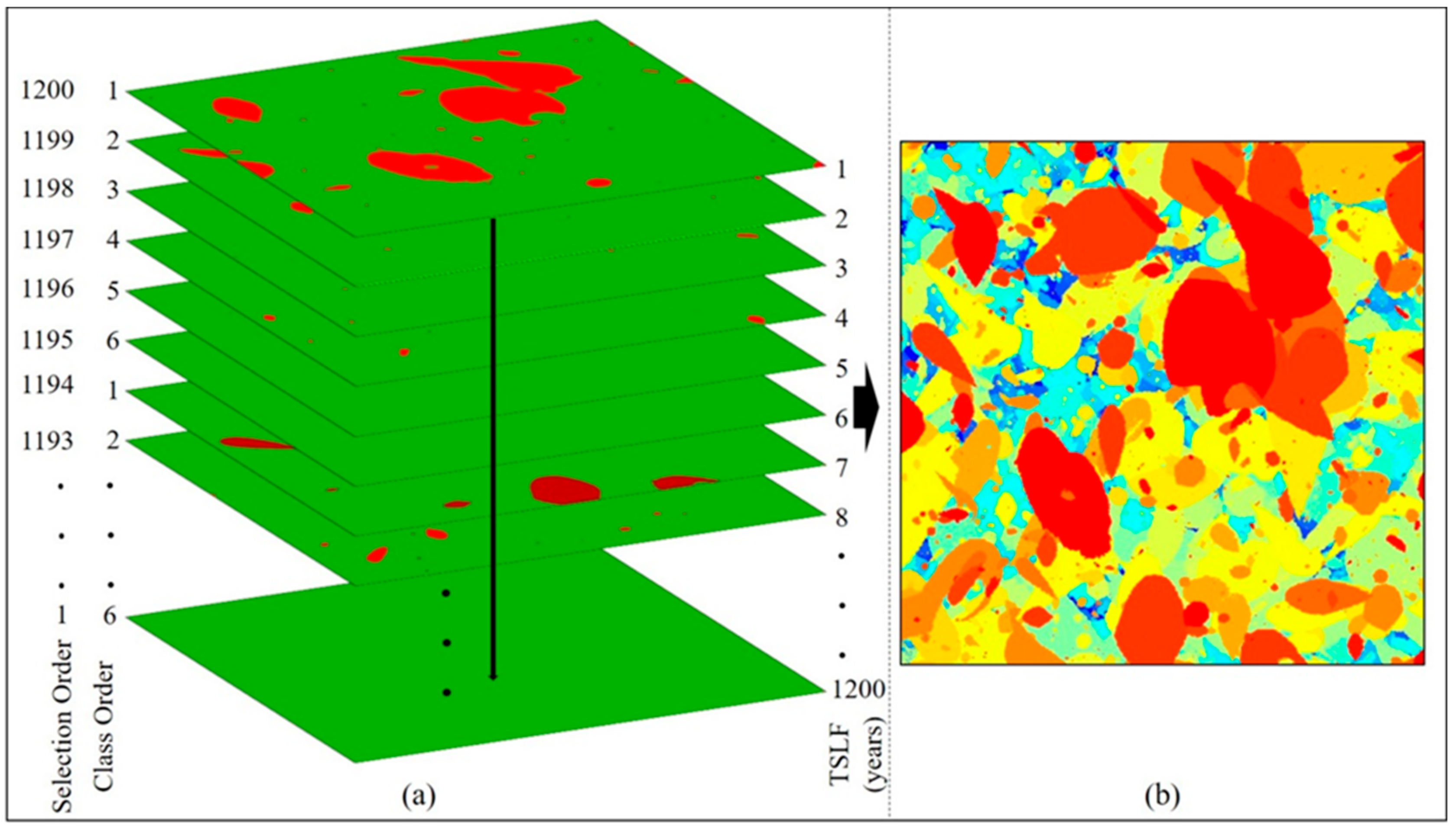
2.5. Time Since Last Fire (TSLF) Map Creation

We simulated 200 years of fires in each of the six classes of total annual area burned, for a total of 1200 years. Since most of the individual fires in Class 6 years were smaller than the cell size of 0.01 km2, we simply used a “no fire” map to represent total annual area burned in those years. Thus, there were actually 1000 years of simulated fires.
TSLF maps were created by overlaying the 1200 maps of total annual area burned in the following sequence of classes of total annual area burned: 6, 5, 4, 3, 2, 1, 6, 5, 4…1 until all 1200 maps had been stacked (Figure 2). The stacking operation was undertaken using a program we wrote in Python. Each annual fire-year map was randomly selected (without replacement) from the appropriate class of total annual area burned, until all 1200 fire-year maps had been selected. The first-used fire-year map represented 1200 years ago, the second-used fire-year map represented 1199 years ago, and the last-used fire-year map represented one year ago. When cells burned in earlier years were overlaid (i.e., over-burned) by more recent fires, their age changed to that of the newer burn.

2.6. Creating TSLF Maps with Different Fire Rotations (FRs)

TSLF maps with a range of FRs were created by leveraging the independence of the 1200 fire-year maps with which they were built, and the influence that the largest fire-years have on the FR [44]. We created a total of 201 TSLF maps that contained progressively fewer of the large, Class 1 fire-year maps: 200, 198,197 … 2, 1, 0. To insure that the 201 TSLF maps were unique in their spatial pattern of fires, they were each created using a new random sequence of fire-year maps (described in Section 2.5). Once stacked, j of the Class 1 fire-year maps were removed by first dividing all fire-year maps into j intervals, and then removing one randomly chosen Class 1 fire-year map from each of the j intervals. This was done for j = 1, 2, 3 … 200. By removing the 200 Class 1 fire-year maps in this strategic manner, we ensured that we would obtain TSLF maps that would have a wide variety of FRS.
Uniqueness of the spatial pattern of forest ages in the TSLF maps was evaluated by comparing TSLF ages in the 11 TSLF maps that contained 200, 180 … 20, 0 of the Class 1 fire-year maps. The 11 TSLF maps had their 2100 × 2100 grid overlain with a lattice which contained 900 nodes that were each separated by 68 grid-cells. The 900 nodes were at the following XY grid-pairs: 68–68, 68–136, 68–204 … 136–68, 136–136 … 2040–2040. The TSLFs at those 900 nodes were extracted from each of the 11 TSLF maps. Spearman rank correlation coefficients were calculated between all pairs of the 11 node-constrained arrays of TSLFs, and the frequency distribution of those 55 paired correlations was examined. Spatial autocorrelation in the 11 TSLF maps was evaluated using the global Moran’s I [47].

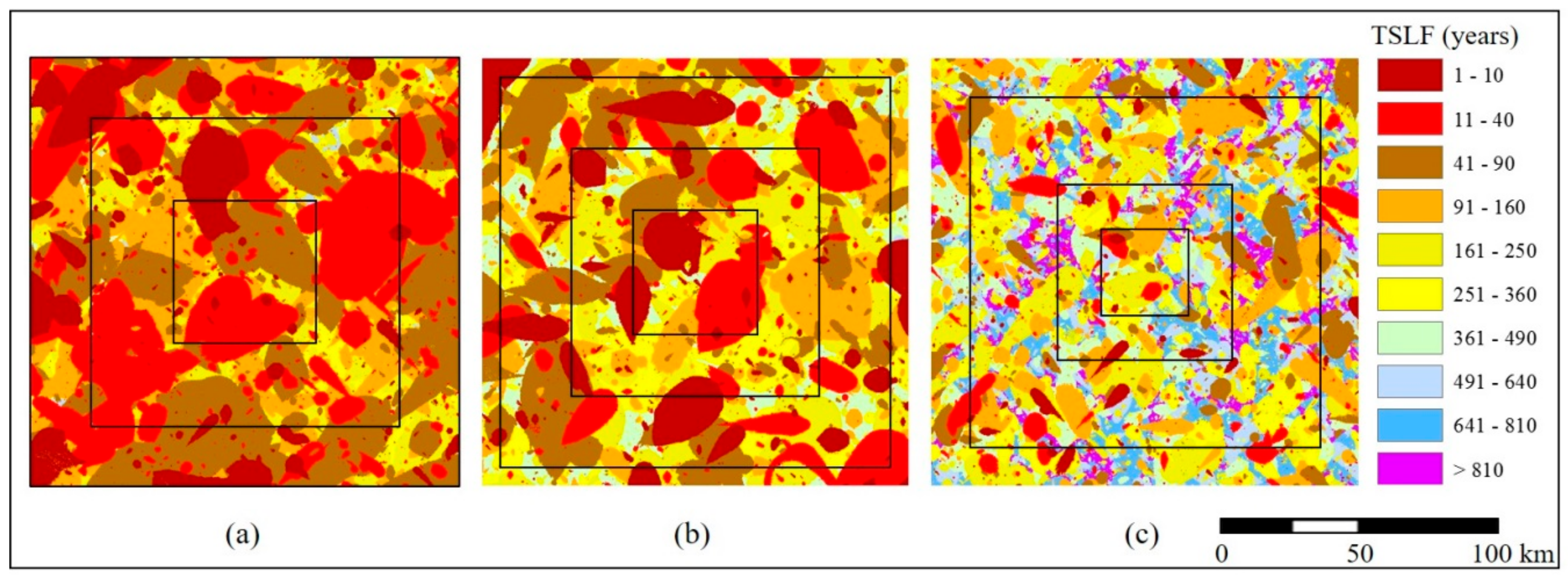
2.7. Creating TSLF Maps at Different Study Area Scales

To assess the influence of study area scale, the 201 TSLF maps with different FRs (see Section 2.6) were evaluated at nine different study area scales. The scales were of the study area size relative to the largest historical total annual area burned. For example, the 2100 × 2100 grid simulated landscape is 6× larger than the largest total annual area burned in the 1200 years of fire simulations (see Section 3.1). The nine scales of 6×, 5×, 4×, 3×, 2×, 1×, 0.75×, 0.50× and 0.25× were created by extracting a square area centered on the middle of the 2100 × 2100 grid simulated landscape (Figure 3). The nine TSLF maps at the different scales were thus nested, but not unique.

2.8. Fire Rotation (FR) and Fire Cycle (FC) Estimation Methods

Fire rotation (FR) is calculated using annual fire maps: study area size divided by the mean total annual area burned. The historical fire rotation (FRH) for WBNP was calculated using its 44-year historic record. The simulated fire rotation (FRS) for the 2100 × 2100 grid simulated landscape was calculated using its 1200 simulated annual fire-year maps. A Python program was written to conduct a Monte Carlo simulation to estimate the mean FRS and its standard deviation. The Python program randomly selected without replacement 100 of the 200 annual fire maps in each of the six classes, and then used those 600 maps to calculate one FRS; this operation was repeated 1000 times providing 1000 estimates of the FRS from which the mean and standard deviation were calculated.
The FC of the TSLF map created using all 1200 annual fire-maps was calculated using two methods: the mean age (FCMA), and the maximum likelihood estimate (FCMLE). The FCMA was estimated as the mean age of 1000 TSLF sample-points; the FCMA was introduced as a simple MLE of a TSLF distribution with a negative exponential form [3]. The FCMLE of 1000 TSLF points was estimated using a more elaborate maximum likelihood function [48] that accounted for two sources of randomness: the random occurrence and spread of fires, and the random selection of sample-points [49]. The 1000 points used to calculate FCMA and FCMLE were distributed across the landscape of the TSLF map in a structured random approach: discretizing the landscape into 100 equal-sized non-overlapping areas of 210 × 210 grid (441 km2), and then obtaining the TSLF from 10 different randomly selected, without replacement, cells from each of the 100 areas. For both methods of estimating the FC, the historical hazard of burning in the simulation would be constant, because the six classes of total annual area burned that we employed would simply cause a six-year cycle around a multi-century trend. The two methods were employed 1000 times. Differences between estimates of FRS, FCMA and FCMLE were assessed using a two-sample t-test.

2.9. Estimating the Minimum Required Number of TSLF Sample-points

To assess the minimum number of sample-points required to estimate the FCMA at a given level of accuracy, we wrote a Python program to conduct a five-step procedure. First, the TSLF map was discretized to obtain 100 square grids numbered 1 to 100. Second, 1000 sample-points were randomly selected in a repeated sequence from the grids 1 to 100; reaching 1000 points required 10 cycles through the 100 grids. Third, each time a new sample-point was added, the FCMA was recalculated, until FCMA was estimated with 1000 sample-points. FCMA was estimated as the sum of TSLF ages for the n points divided by n. Fourth, the number of sample-points required to estimate mean FCMA at a given level of accuracy was determined by the absolute difference in the measured mean (ADMM):
ADMM = a b s ( i = 1 n A g e S o r d e r M e a n A g e ( 1000 ) ) M e a n A g e ( 1000 ) × 100
where abs is the absolute value, MeanAge(1000) is the mean of the 1000 randomly selected sample-points, and Sorder is the order of the 1000 samples. Accuracy in this study was assessed using an ADMM threshold of 10%, but the program can be modified to employ any value. Fifth, the minimum sample size was identified as the lowest sample size at which the ADMM stayed lower than the threshold value of 10% for the remainder of the 1000 sample-points. The 1000 different estimates of the minimum sample size were then expressed as their 95th percentile.

2.10. Influence of Study Area Scale on Estimated FC and TSLF Age Variability

The influence of study area scale (study area size divided by largest total annual area burned) on FCMA estimation was evaluated in four steps. First, the FRs was calculated for all 201 TSLF maps for the whole 2100 × 2100 grid landscape. Since FRs was calculated using all of the individual fire-year maps that were used to create the TSLF map, FRs provides the “true” value that a good estimate of FCMA should also provide. Second, FCMA was estimated for all 201 TSLF maps at all nine scales, for a total of 1809 values. Third, at each of the nine scales, the root mean square error (RMSE) and R2adj were calculated between the 201 FRS values and FCMA estimates. Fourth, the RMSE and R2adj values were graphed across the nine scales to assess if there was a scale at which the FRS and FCMA no longer agreed well.
The influence of study area scale on age variability across TSLF maps was evaluated in four steps. First, the FRs was calculated for all 201 TSLF maps for the whole 2100 × 2100 grid landscape. Second, 1000 TSLF points were selected from each of the 1809 TSLF maps and their standard deviation was calculated; this was done 1000 times for each map and their mean was calculated. Note: in a negative exponential distribution, the standard deviation and the mean should have equal values [3]. Third, at each of the nine scales, the RMSE and R2adj were calculated between the 201 FRS values and the standard deviation of the TSLF ages. Fourth, the RMSE and R2adj values were graphed across the nine scales to assess if there was a scale at which the two measures indicate poor agreement between FRS and the standard deviation.

2.11. Influence of FRS and Study Area Scale on Minimum Required Sample-Points

The influence of the FRS on the accuracy of the FCMA estimate was evaluated in three steps. First, the value of FRS minus FCMA (i.e., FRS-FCMA) was calculated for all 201 TSLF maps at all nine scales, for a total of 1809 values. FRS was always for the whole 2100 × 2100 grid landscape, as it represents the basic conditions behind the creation of the TSLF map. Second, linear regressions were conducted between the 201 values of FRs against FRs minus FCMA, with this done separately for each of the nine scales. Third, the intercept and slope parameters and p-values were tabulated; study-area scales at which the intercept and slope were not significantly different than zero were inferred to have had no influence on the length or the FRS on the length of the FCMA estimate.
The minimum number of TSLF samples required to estimate FCMA at a given level of accuracy was assessed using four steps. First, for each of the 201 TSLF maps at each of the nine scales we determined the 95th percentile of the minimum number of TSLF sample-points required to obtain an ADMM of 10% (see Section 2.9). Second, those values were expressed in two ways: the number of TSLF points per map and, since the nine study area scales differed greatly in total area, the number of TSLF points per 100 km2. Third, linear regressions were conducted between the 201 values of FRS against the 95th percentile of the minimum number of sample sizes for each of the 201 maps; this was done separately at each of the nine scales. The FRS was for the whole 2100 × 2100 grid landscape. Fourth, the 95th percentile of the 201 minimum sample values was calculated for each of the nine scales and graphed.

3. Results

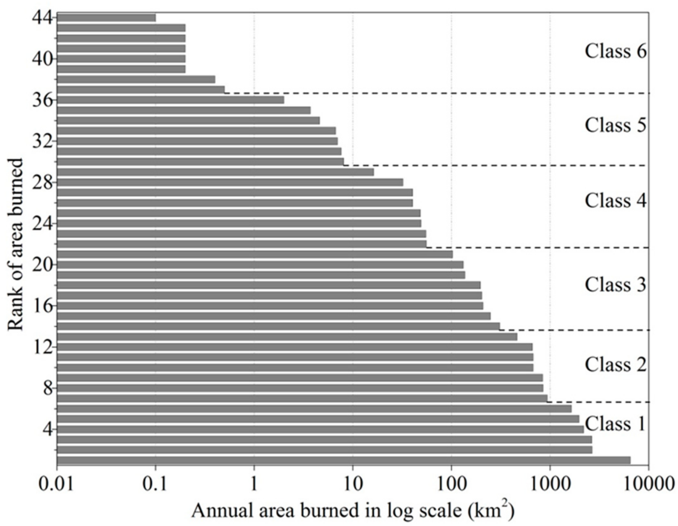
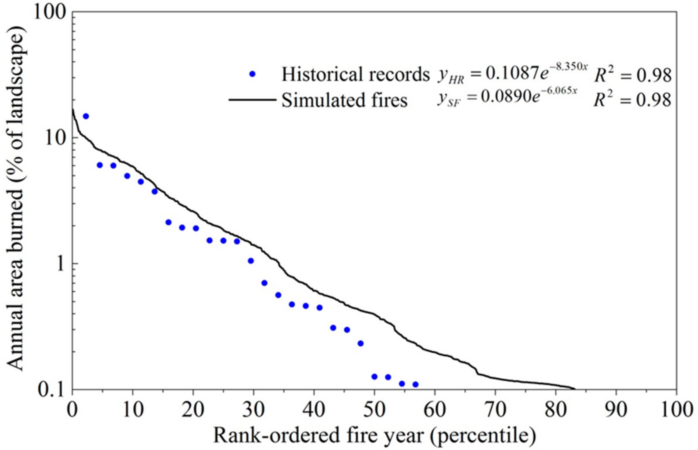
3.1. Simulated Fires and Fire-Year Maps

The largest simulated fire in the 1200 fire-year maps was 1562 km2 (Table 1; 3.5% of the simulated landscape). The largest of the 1200 simulated fire years burned 7385 km2 (16.7% of the landscape), and the mean total annual area burned for the 1200 fire maps was 717.5 km2. The fire characteristics in the six classes of total annual area burned was similar for the 1200 years of simulated fires as it was for the 44 years of historical fires (Table 1) in terms of both the absolute size of the largest individual fire, as well as the mean percent of the landscape burned annually and the percent of the total area burned.
Rank-ordered distributions of the total annual area burned in the 1200 years of simulated fires and the 44 years of historical fire records both exhibit a negative exponential distribution (Figure 4). The distributions are more similar for large fire years than for small fire years; for example, the largest 30% of the historical fire years and the largest 34% of the simulated fire years each burned >1% of the study area per year. The historical data exhibit a steeper slope in the frequency of total annual area burned than do the simulated data. The Monte Carlo estimate of FRS from the 1200 fire-year maps was 61.5 years (range: 57.6 to 66.3 years).

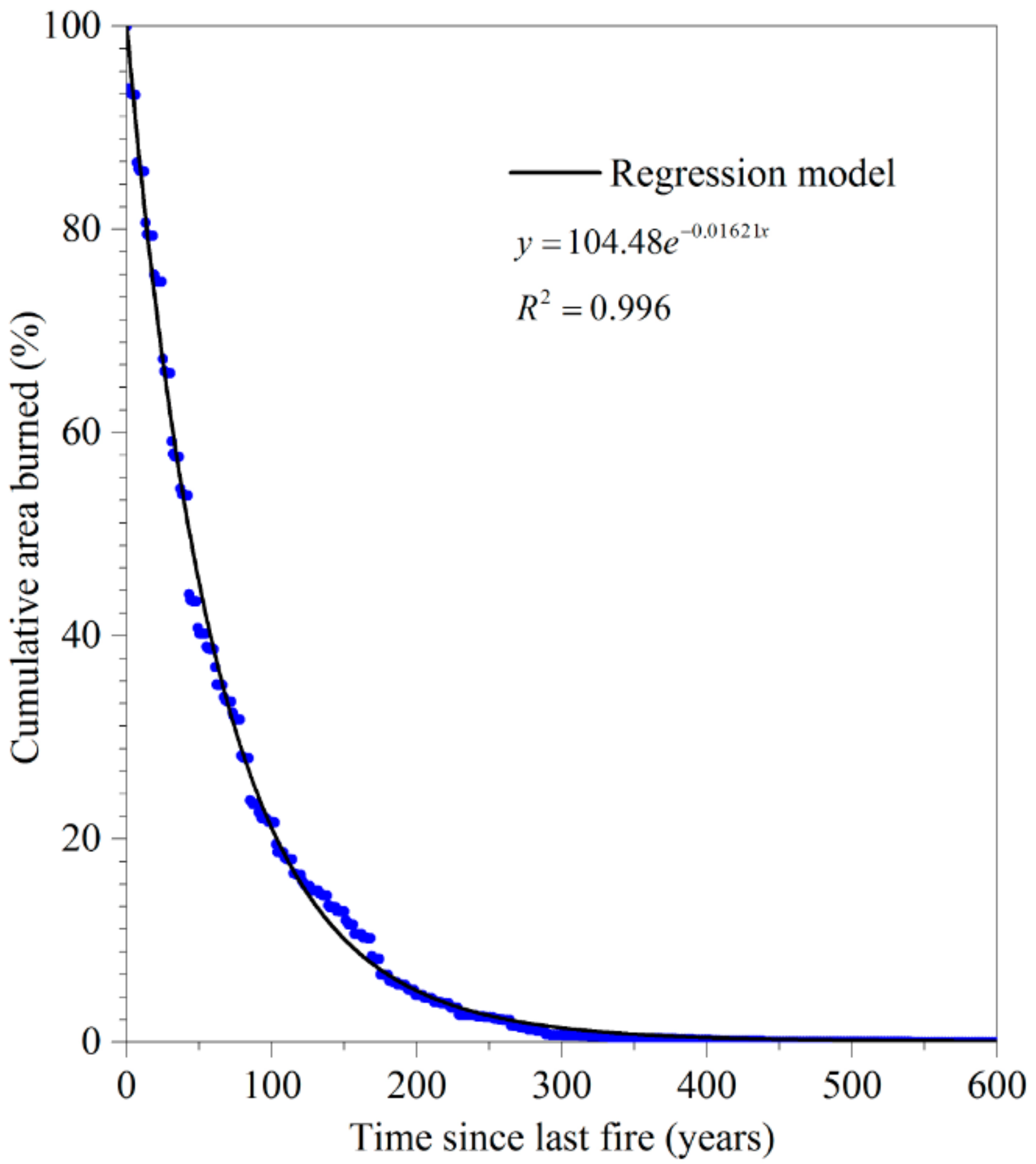
3.2. Time Since Last Fire Map and FC Estimates Using Initial Fire Parameters

The TSLF map for the 2100 × 2100 grid landscape, created using 1200 fire-year maps based on the fire parameters in Table 2, contains much young forest and progressively less old forest (Figure 3a). The cumulative frequency distribution of TSLFs for all 4,410,000 cells from that TSLF map (Figure 3a) displays a negative exponential distribution (Figure 5), the slope of which indicates a FC of 61.7 years. When 1000 TSLF points were sampled from that TSLF map 1000 times, the mean FC was 61.6 years for FCMA (range: 57.9 to 66.9 years), and 61.7 years for FCMLE (range: 57.0 to 66.3 years). The FCMA was not significantly different from FCMLE (p = 0.35) or FRS (p = 0.18; from Section 3.1), as indicated by two-tailed t-tests.

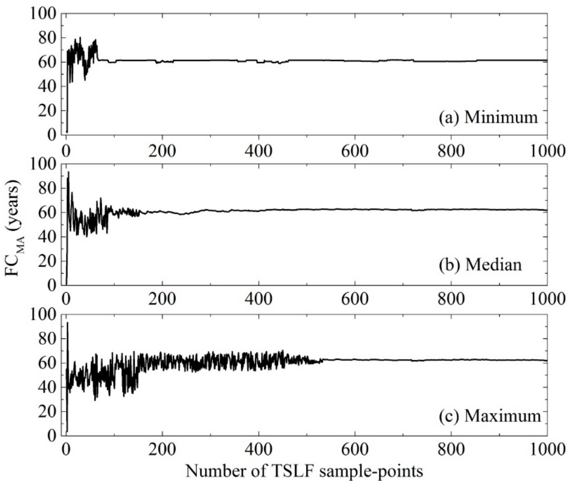
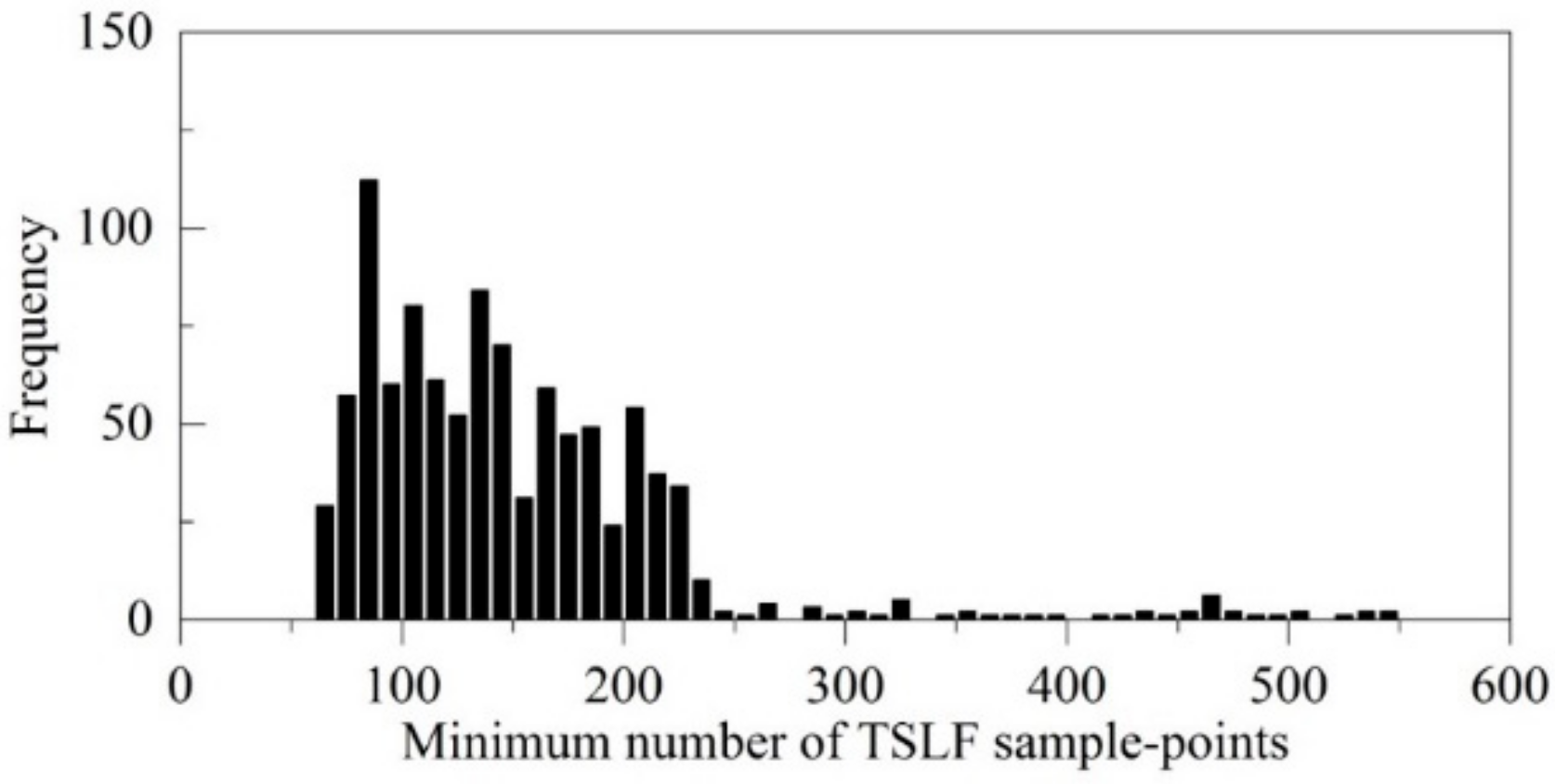
3.3. Examples of Calculating the Minimum Number of Sample-Points

With an increase in the number of sample-points from the TSLF map (Figure 3a, created using all 1200 fire maps and the 2100 × 2100 grid landscape) the FCMA estimate initially varied greatly and then stabilized (Figure 6). When an ADMM of 10% was employed 1000 times from this TSLF map, the minimum number of samples required ranged from 65 to 571, with a median of 147 and a 95th percentile of 239 sample-points (Figure 7).

3.4. Creation of TSLF Maps with Different FRS

The 201 TSLF maps had an FRS that ranged from a low of 61.1 years when all 200 Class 1 fire years were employed, to a high of 200.5 years when no Class 1 fire years were employed. TSLF maps with fewer Class 1 fire years had progressively less young forest and more old forest (Figure 3). Spearman rank-correlations between 55 permutations of 11 TSLF maps ranged from −0.164 to 0.343 with a median of 0.026; when classified into bins that were 0.05 correlation-units wide, the mode was in the zero-bin of −0.024 to 0.025. The global Moran’s I ranged from −0.127 to 0.120, and was positively correlated with FRS for those maps (rs = 0.964, p = 0.0000, n = 11), but not correlated with the 95th percentile of TSLF sample-points for those maps (rs = −0.092, p = 0.789, n = 11).

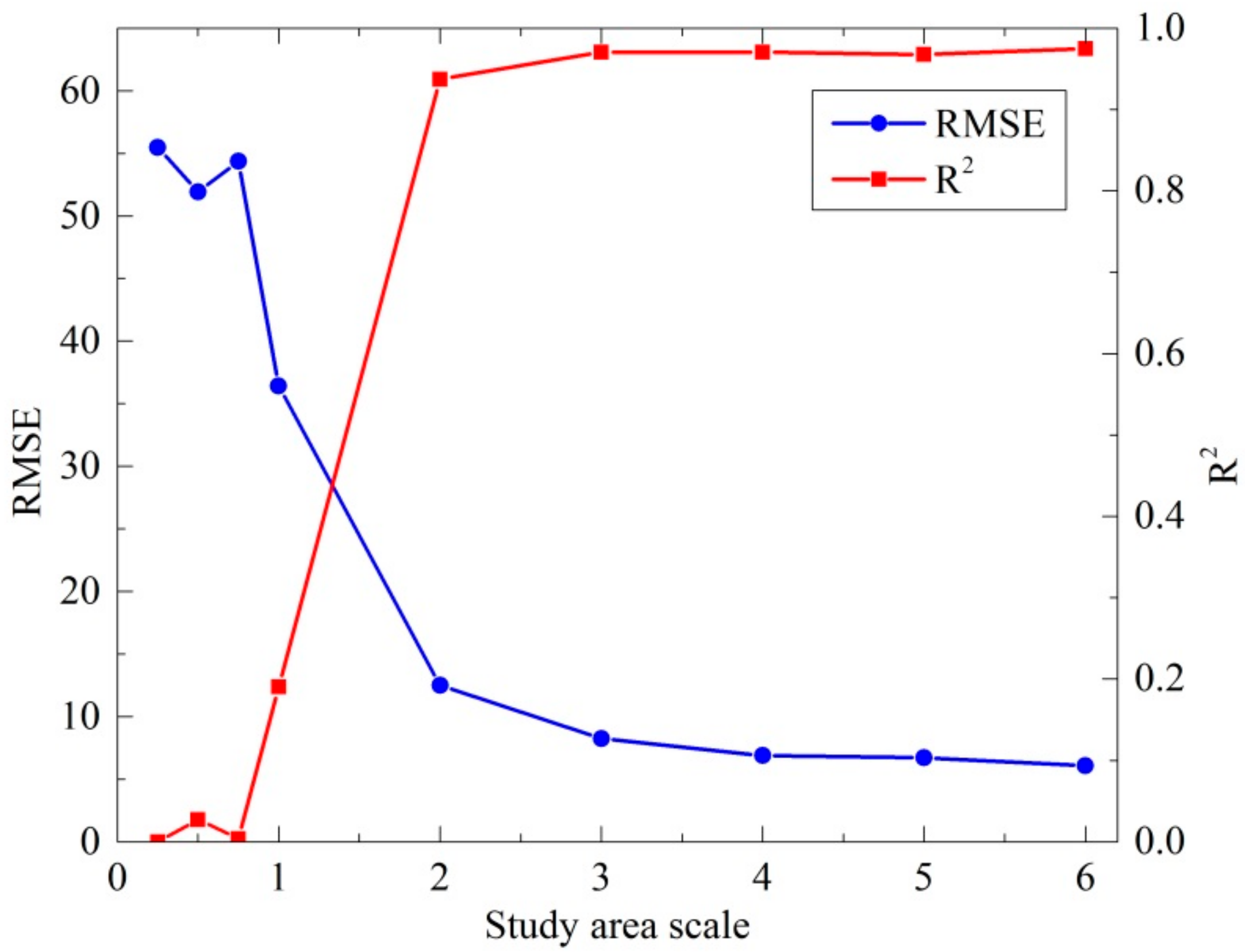
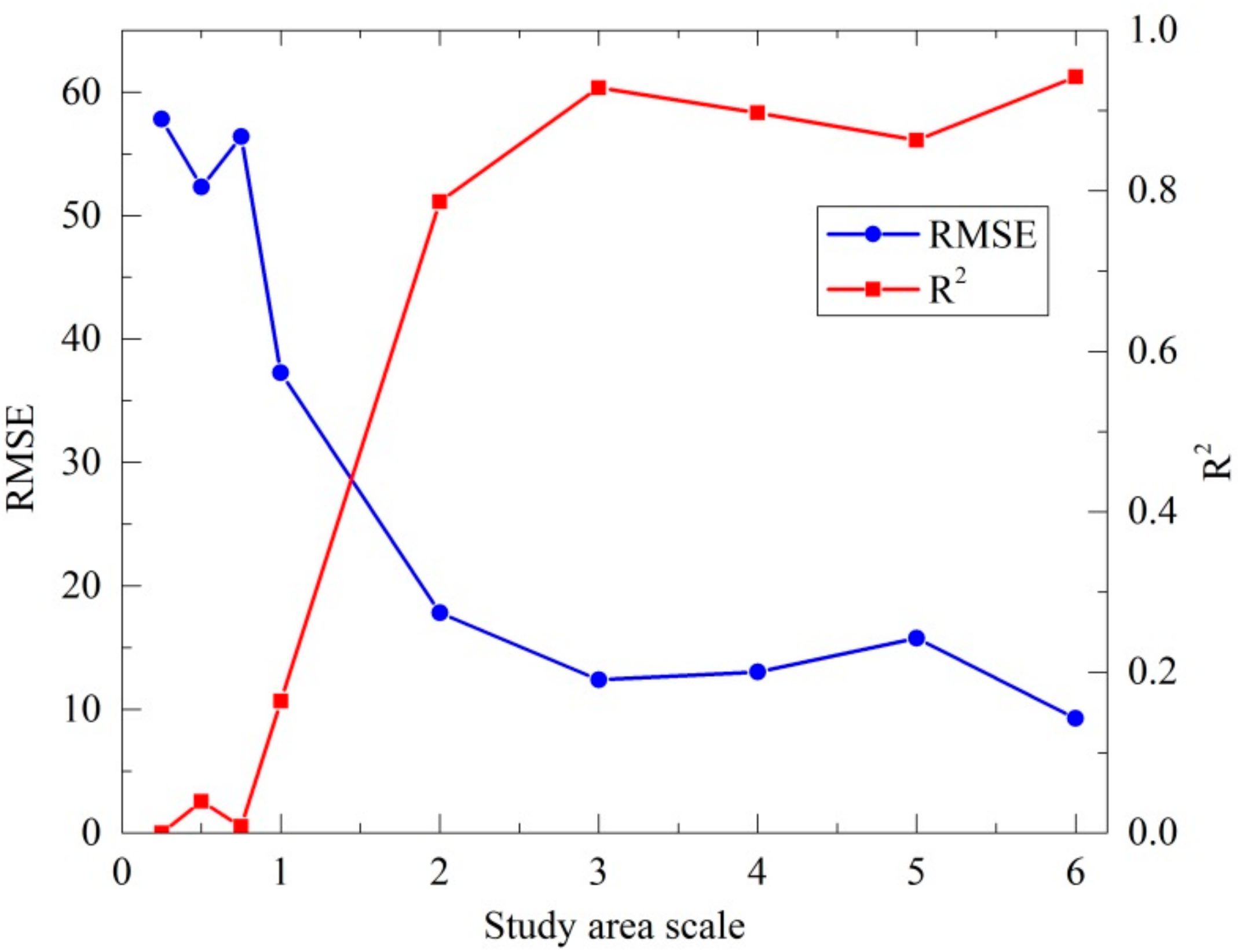
3.5. Influence of Study Area Scale on Estimated Fire Cycle (FCMA) and TSLF Age Variability

At a study area scale of 3× of the largest total annual area burned, TSLF maps based on a higher FRS also had a higher FCMA estimated from the TSLF map (Figure 8). In contrast, at a study area scale of 0.5×, TSLF maps based on a higher FRS did not yield higher FCMA estimates. When those calculations were done for all nine scales (Figure 9), TSLF maps with a study area scale of ≥2× had a high R2adj and low RMSE between FRS and FCMA, while scales of ≤1× had a low R2adj and high RMSE. When similar analyses were conducted between the FRS and the standard deviation of the 201 TSLF maps (Figure 10), TSLF maps with a study area scale of ≥2× had a high R2adj and low RMSE between FRS and standard deviation, and study area scales of ≤1× had a low R2adj and high RMSE.

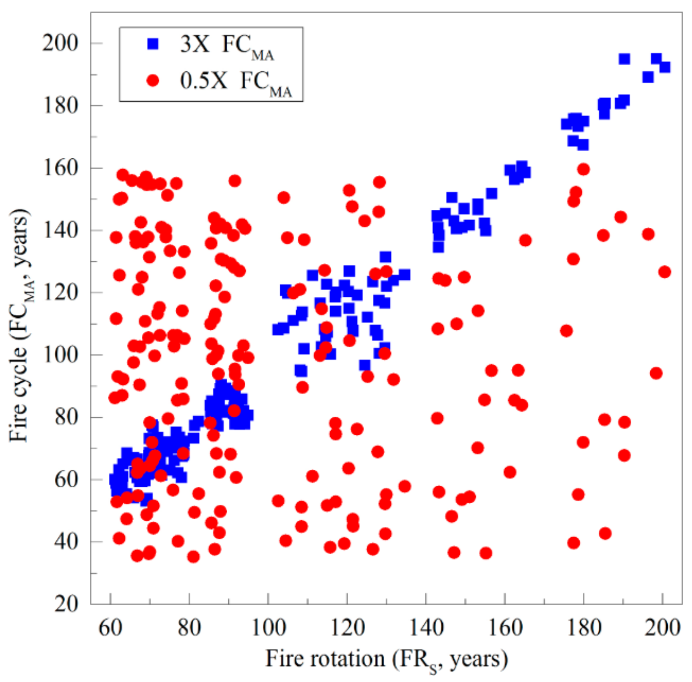
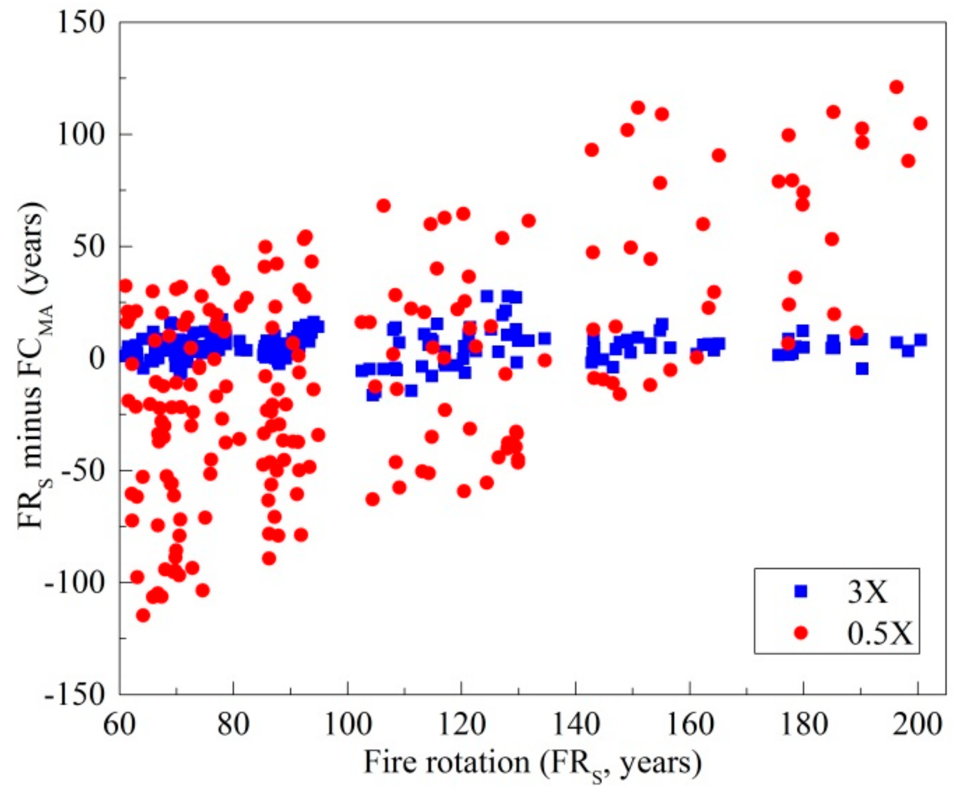
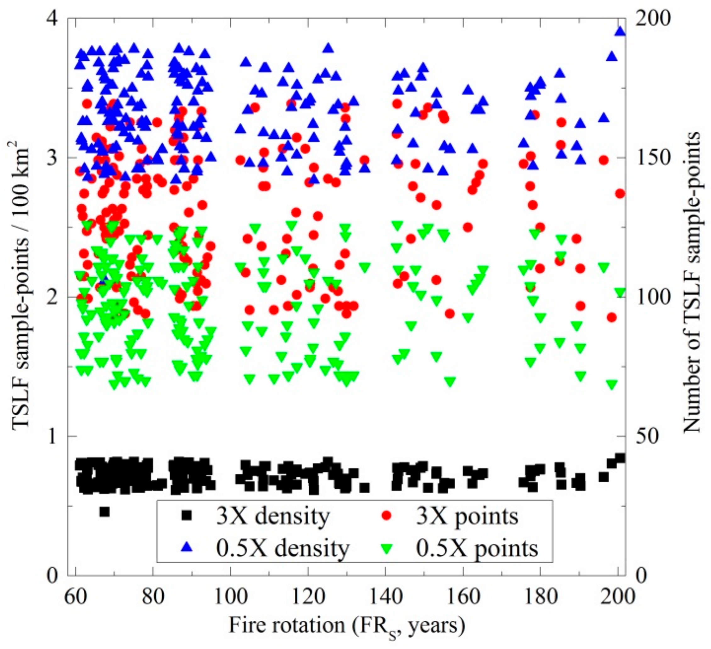
3.6. Influence of FR and Study Area Scale on Minimum Required Sample-Points

At a study area scale of 3× of the largest total annual area burned, TLSF maps based on a longer FRS did not exhibit any difference between FRS for the whole study area and FCMA estimates from the 3× scale TSLF map (Figure 11). In contrast, at a study area scale of 0.5×, TSLF maps based on a longer FRS did exhibit differences between FRS for the whole study area and FCMA estimates from the 0.5× scale TSLF map; the differences were typically negative for low values of FRS and positive for high values of FRS. Results from linear regressions between FRS and the FCMA from the nine different scales (Table 3) indicate that scales ≥4× had intercept values that were not different than zero, while progressively smaller scales had progressively more negative intercepts. The regression results also indicate that scales ≥3X had slopes that were not significantly different than zero, while progressively smaller scales had steeper slopes that were significantly different than zero.
At a study area scale of 3× of the largest total annual area burned, TSLF maps based on a longer FRS did not require more TSLF sample-points to obtain an ADMM of 10% than did TSLF maps based on a shorter FRS (Figure 12). There was no significant trend with FRS in the number of sample-points for the 0.5× study area, nor for the density of sample-points for the 3× or 0.5× study areas. The 3X study area scale did require more TSLF total sample-points, but at a lower density of sample-points per 100 km2, than did the 0.5× study area scale. In general, an increase in study area scale resulted in a linear increase in the minimum total number of required TSLF sample-points, and a negative exponential decrease in the number of sample-points per 100 km2 (Figure 13).

4. Discussion

Our key findings suggest that: TSLF fire histories should employ study areas ≥3× the largest total annual area burned [7]; the minimum number of TSLF sample numbers and sample density that should be employed differs with study area scale (study area divided by largest total annual area burned); and an influence of FRS length on the FC estimate only occurs if the study area scale is <3×. Although the 201 TSLF maps were created by randomized resorting of the same 1200 simulated fire-year maps, Spearman correlations suggest that the TSLF maps contain unique spatial patterns. Our results most directly apply to areas of boreal forest that are predominantly burned by large stand-replacing fires, but scaling relations could be used as a first approximation for study areas with small stand-replacing fires.
Three aspects of our results support the suggestion that study areas should be ≥3× the size of the largest total annual area burned [7]. First, relations between FRS and the FCMA are best for scales of ≥2×. That is, for study area scales ≥2×, the estimated FCMA was strongly similar to the FRS for the complete 2100 × 2100 grid simulated landscapes. Remember that since the TSLF map is based on the FRS, a good FCMA estimate should equal the FRS. Second, the individual regressions between FRS against FRS minus FCMA at each study area scale indicate that only scales of ≥4× had an intercept not different than zero, and only scales ≥3× had a slope not different than zero. Third, standard deviation in TSLF ages is most similar to FRS for scales of ≥2×. Since a fundamental property of the negative exponential distribution that many TSLF distributions display, is that the mean and standard deviation should have equal values, it is not surprising that our scaling results were similar for the two parameters. Thus, while our results suggest that a study area scale as small as 2× could provide accurate estimates of the FC, since some of our relations only become stable at 4×, our findings agree with others that progressively larger areas provide more accurate results [14,15,16]. Also, since a small study area scale will likely provide a TSLF distribution that is not representative of the FR, increasing the number of TSLF sample-points cannot fix that misrepresentation.
Given that real landscapes contain spatial heterogeneity in environmental conditions, unlike our spatially homogenous simulated area, study area scales >3× are likely required to obtain accurate FC estimates [50]. Of the 18 TSLF fire history studies whose size and sample numbers were given in the Introduction, five provided information on the largest total annual area burned; they had a median study area scale of 4.1 and a range from 1.7 to 16.2 [8,22,27,28,32]. This suggests that TSLF fire history studies should, to reduce possible errors in their results and to maximize the interpretive potential of their data, strive to study larger areas. In study areas restricted by property boundaries such as the edge of a park that make larger study area scales infeasible, recognition should be made that the FCMA could misrepresent the real FC even if the TSLF sample size is high.
The number and density of TSLF samples required to estimate the FC with an error (ADMM) of less than 10% for study area scales of 3× were, respectively, 187 samples and 0.81 per 100 km2. While this coarse-scale sampling will provide information on the regional FC, it will not provide enough information to understand small-scale drivers. An increase in sample number or density would help with detecting environmental small-scale drivers of spatial variations in FC, e.g., [18,27]. If we assume that the 18 TSLF-based fire history studies mentioned in the Introduction had a study area scale of 3×, then two of them did not meet the sample density requirement, and nine did not meet the sample number requirement. This indicates that increased TSLF sample sizes should be employed to reduce error in FC estimates.
Our results suggest that only study areas with a scale of <3× will have FC estimates influenced by the length of the FR. In general, small-scaled areas with a short FR have an overestimated FC, and small-scaled areas with a long FR have an underestimated FC. This pattern is supported by the only studies we are aware of that allow a multi-scale comparison of FC and FR: the FC of 47 years from a 1.1× scaled study area by Van Wagner [3] underestimates the FR of 204 years calculated from a 2.3× scaled study area by Heinselman [8] within which it was nested.
The reduced standard deviation of TSLF ages that we observed in smaller areas could result in uncommon old stands over-influencing the FC estimate in areas with a short FR, and uncommon young stands over-influencing the FC estimate in areas with a long FR. It is possible, however, that field-based TSLF studies could avoid those biases as the exact area of recent burns can be known from historical records and/or remotely sensed imagery, and very old burns would be lost due to mortality of the original tree cohort and be replaced by younger successional forests, e.g., [13].
We recognize that our simulation methods and study design have some limitations, and could be improved in four key regards. First, our uniform landscape did not consider spatial variation in factors such as soil, topography, hydrography and climate, known to influence FC [27,51]. Future studies could assess how requirements of study area scale and TSLF number change with increased spatial heterogeneity. Our preliminary research using neutral landscape models showed that increases in positive spatial autocorrelation did require increased number of TSLF sample points (Supplementary Materials), but variations in spatial autocorrelation in our 11 TSLF maps did not appear to influence the required number of TSLF sample points. A second improvement would involve modifying LANDIS-II and DFSS (Dynamic fuels and fire system) so that each simulated year could sample from different probability distributions of fire occurrence, fire size and fire weather. Since our preliminary analyses showed that using only one set of fire parameters resulted in unrealistically low inter-annual variation in area burned, we employed six classes of fire parameters and thus had to simulate years individually. If LANDIS-II and DFSS included this modification, that would allow one TSLF map to develop over 1200 years of burning, and thus incorporate the influences of forest age on fire spread [52]. Third, our TSLF maps did not assume censoring due to mortality, and thus unrealistically contained TSLF grids >801 years. We could have applied a censoring to TSLF points, e.g., [13] but we instead believe that fire history field researchers should examine tree-rings to determine if it is an open-grown post-fire stand, or a closed-grown successional stand [53]. If the latter occurs then either soil charcoal should be used to get the TSLF, e.g., [54], or the TSLFs should be examined as a truncated distribution [7].
A fourth improvement would be to evaluate the influence of age-related changes in the hazard of burning on the required number of TSLF sample-points. Many but not all forest types exhibit an increase in the hazard of burning with increased age [55] which can cause increased positive spatial autocorrelation of TSLF [52]. Since increasingly positive spatial autocorrelation requires an increased number of sample-points to obtain a spatially representative mean value of landscape conditions [56], forests that have age-related increase in the hazard of burning might require more TSLF sample-points. Indeed, in a preliminary evaluation of this issue using neutral landscape models, we found that increases in spatial clustering of forest ages, such as might occur due to age-related increases in hazard of burning, did result in an increase in the required number of TSLF sample-points (Supplementary Materials).
We suggest six different ways that future TSLF fire history studies could apply our results to estimate the FC in forests with a stand-replacing fire regime. First, and most importantly, researchers should always use a study area ≥3× the largest total annual area burned. If the study area is under fire suppression, then they should use the largest total annual area burned from pre-suppression TSLF records or from other fire history studies. Second, researchers could use the minimum number of TSLF sample-points that we suggest for the relevant study area scale. Third, researchers should increase the number of TSLF sample-points above our minimum to account for spatial and temporal heterogeneity, such as caused by age- or environment-related increases in the hazard of burning (Supplementary Materials). Fourth, researchers could divide our TSLF sample density requirement by the appropriate scaling factor related to largest total annual area burned. For example if a study area had the largest total annual area burned 1/10 that in our study area, then instead of 0.81 samples per 100 km2 they would use 0.81 samples per 10 km2. This approach does, however, simplistically assume similar slopes of the total annual area burned distributions. Fifth, researchers could import their spatial environment into LANDIS-II and DFSS, and parameterize the simulations in a manner that would reflect that area’s temporal variations in fire weather. They could then use our Python code to determine either the number of TSLF points required to reach an acceptable error, or determine the error their FC estimate will have given their constraints in study area and sample number. Since all study areas contain unique spatial patterns of environmental factors that influence the hazard of burning, and unique age-related changes in the hazard of burning, this approach will yield the most realistic indication of the required number of TSLF sample-points. Sixth, an ongoing TSLF fire history could begin with our minimum suggested sample density, and employ a Monte Carlo simulation while doing fieldwork to estimate the FC and the error in that estimate; if the error is too high then the researchers would gather additional TSLF samples until the error was acceptable.

5. Conclusions

The method of constructing and sampling TSLF maps that we developed allows guidelines to be tested in regard to how large of a study area and how many TSLF sample-points should be employed to estimate the FC using the TSLF method. This approach builds upon previous simulation studies which showed that increased sampling effort would reduce error in FC estimates.
Our results indicate that TSLF fire histories should be created for areas that are ≥3× the largest total annual area burned that occurs in the region within which the study area is located. If smaller study areas are employed, then areas with a short but unknown FR will likely obtain an overestimated FC, and areas with a long but unknown FR will likely obtain an underestimated FC. Since these biases will be the result of the study area being too small, they cannot be compensated for by employing more TSLF samples.
Our results further indicate that in forests whose fire regime is similar to our simulation, 187 TSLF sample-points is the minimum required to estimate the FC with an error of less than 10% in a study area 3× the largest total annual area burned. Larger areas would require more samples but at a lower spatial density. Since our suggestions are based on a spatially homogenous study area with a cyclic climate, study areas with progressively higher spatial and temporal heterogeneity due to factors such as age-related increases in the hazard of burning, should employ progressively more TSLF samples. To optimize the number of TSLF samples in a fire history study, we encourage researchers to develop site-specific applications of our simulation approach prior to conducting fieldwork.

Supplementary Materials

All input data and code from this study are available at XW’s Github repository: https://gist.github.com/xinyuanwylb19. A supplementary section is available at https://0-www-mdpi-com.brum.beds.ac.uk/1999-4907/9/11/708/s1: “A preliminary evaluation of the influence of environment- and age-related spatial autocorrelation on the required number of time since last fire sample-points”.

Author Contributions

C.P.S.L. conceived the research idea. X.W. designed and performed the simulations. X.W. and C.P.S.L. contributed equally to analyses of data. X.W and C.P.S.L. contributed equally to creation of figures. X.W. and C.P.S.L. contributed equally to writing of the manuscript.

Funding

This research received no external funding.

Acknowledgments

We thank D. Scott Mackay and two anonymous reviewers for helpful comments on earlier versions of this manuscript, the University at Buffalo Center for Computational Research for supercomputing resources, Daniel J. Hayes of the University of Maine for providing additional supercomputing resources, and the University at Buffalo Department of Geography for helping with publication costs.

Conflicts of Interest

The authors declare no conflict of interest.

Abbreviations

The following abbreviations are used in this manuscript:
ADMMAbsolute difference in the measured mean
DFSSDynamic fuels and fire system
FCFire cycle
FCMAFire cycle estimated as mean age of simulated TSLF map
FRFire rotation
FRHFire rotation estimated from historical data
FRSFire rotation estimated from simulated data
LANDIS-IILandscape disturbance and succession model, version 2
MFIMean fire interval
MLEMaximum likelihood estimator
TSLFTime since last fire
WBNPWood Buffalo National Park

References

  1. Giglio, L.; Randerson, J.T.; Van der Werf, G.R.; Kasibhatla, P.S.; Collatz, G.J.; Morton, D.C.; DeFries, R.S. Assessing variability and long-term trends in burned area by merging multiple satellite fire products. Biogeosciences 2010, 7, 1171–1186. [Google Scholar] [CrossRef] [Green Version]
  2. Kloster, S.; Lasslop, G. Historical and future fire occurrence (1850 to 2100) simulated in CMIP5 Earth System Models. Glob. Planet. Chang. 2017, 150, 58–69. [Google Scholar] [CrossRef]
  3. Van Wagner, C.E. Age-class distribution and the forest fire cycle. Can. J. For. Res. 1978, 8, 220–227. [Google Scholar] [CrossRef]
  4. Li, C. Estimation of fire frequency and fire cycle: A computational perspective. Ecol. Model. 2002, 154, 103–120. [Google Scholar] [CrossRef]
  5. Alvarado, S.T.; Fornazari, T.; Cóstola, A.; Morellato, L.P.C.; Silva, T.S.F. Drivers of fire occurrence in a mountainous Brazilian cerrado savanna: Tracking long-term fire regimes using remote sensing. Ecol. Indic. 2017, 78, 270–281. [Google Scholar] [CrossRef]
  6. Larsen, C. Area burned reconstruction and measurement: A comparison of methods. In Biomass Burning and Its Inter-Relationships with the Climate System; Innes, J.L., Beniston, M., Verstraete, M.M., Eds.; Kluwer Academic Publishers: Dordrecht, The Netherlands, 2000; pp. 321–339. [Google Scholar]
  7. Johnson, E.A.; Gutsell, S.L. Fire frequency models, methods and interpretations. Adv. Ecol. Res. 1994, 25, 239–287. [Google Scholar]
  8. Heinselman, M.L. Fire in the virgin forests of the Boundary Waters Canoe Area, Minnesota. Quat. Res. 1973, 3, 329–382. [Google Scholar] [CrossRef]
  9. Polakow, D.A.; Dunne, T.T. Modelling fire-return interval T: Stochasticity and censoring in the two-parameter Weibull model. Ecol. Model. 1999, 121, 79–102. [Google Scholar] [CrossRef]
  10. Reed, W.J.; Larsen, C.P.S.; Johnson, E.A.; MacDonald, G.M. Estimation of temporal variations in historical fire frequency from time-since-fire map data. For. Sci. 1998, 44, 465–475. [Google Scholar]
  11. Rogeau, M.-P.; Armstrong, G.W. Quantifying the effect of elevation and aspect on fire return intervals in the Canadian Rocky Mountains. For. Ecol. Manag. 2017, 384, 248–261. [Google Scholar] [CrossRef]
  12. Finney, M.A. The missing tail and other considerations for the use of fire history models. Int. J. Wildland Fire 1995, 5, 197–202. [Google Scholar] [CrossRef]
  13. Cyr, D.; Gauthier, S.; Boulanger, Y.; Bergeron, Y. Quantifying fire cycle from dendroecological records using survival analyses. Forests 2016, 7, 131. [Google Scholar] [CrossRef]
  14. Karau, E.C.; Keane, R.E. Determining landscape extent for succession and disturbance simulation modeling. Landsc. Ecol. 2007, 22, 993–1006. [Google Scholar] [CrossRef]
  15. Boychuk, D.; Perera, A.H.; Ter-Mikaelian, M.T.; Martell, D.L.; Li, C. Modelling the effect of spatial scale and correlated fire disturbances on forest age distribution. Ecol. Model. 1997, 95, 145–164. [Google Scholar] [CrossRef]
  16. Barclay, H.J.; Li, C.; Hawkes, B.; Benson, L. Effects of fire size and frequency and habitat heterogeneity on forest age distribution. Ecol. Model. 2006, 197, 207–220. [Google Scholar] [CrossRef]
  17. Parisien, M.-A.; Parks, S.A.; Krawchuk, M.A.; Flannigan, M.D.; Bowman, L.M.; Moritz, M.A. Scale-dependent controls on the area burned in the boreal forest of Canada, 1980–2005. Ecol. Appl. 2011, 21, 789–805. [Google Scholar] [CrossRef] [PubMed]
  18. Bélisle, A.C.; Leduc, A.; Gauthier, S.; Desrochers, M.; Mansuy, N.; Morin, H.; Bergeron, Y. Detecting local drivers of fire cycle heterogeneity in boreal forests: A scale issue. Forests 2016, 7, 139. [Google Scholar] [CrossRef]
  19. Bergeron, Y. The influence of island and mainland lakeshore landscapes on boreal forest fire regimes. Ecology 1991, 72, 1980–1992. [Google Scholar] [CrossRef]
  20. Bergeron, Y.; Gauthier, S.; Flannigan, M.; Kafka, V. Fire regimes at the transition between mixedwood and coniferous boreal forest in northwestern Québec. Ecology 2004, 85, 1916–1932. [Google Scholar] [CrossRef]
  21. Cyr, D.; Gauthier, S.; Bergeron, Y. Scale-dependent determinants of heterogeneity in fire frequency in a coniferous boreal forest of eastern Canada. Landsc. Ecol. 2007, 22, 1325–1339. [Google Scholar] [CrossRef]
  22. Drever, C.R.; Messier, C.; Bergeron, Y.; Doyon, F. Fire and canopy species composition in the Great Lakes-St. Lawrence forest of Témiscamingue, Québec. For. Ecol. Manag. 2006, 231, 27–37. [Google Scholar] [CrossRef] [Green Version]
  23. Engelmark, O. Forest fires in the Muddus National Park (Northern Sweden) during the past 600 years. Can. J. Bot. 1984, 62, 893–898. [Google Scholar] [CrossRef]
  24. Grenier, D.J.; Bergeron, Y.; Kneeshaw, D.; Gauthier, S. Fire frequency for the transitional mixedwood forest of Timiskaming, Québec, Canada. Can. J. For. Res. 2005, 35, 656–666. [Google Scholar] [CrossRef]
  25. Johnson, E.; Fryer, G.; Heathcott, M. The influence of man and climate on frequency of fire in the interior wet belt forest, British Columbia. J. Ecol. 1990, 403–412. [Google Scholar] [CrossRef]
  26. Johnson, E.A.; Larsen, C.P.S. Climatically induced change in fire frequency in the southern Canadian Rockies. Ecology 1991, 72, 194–201. [Google Scholar] [CrossRef]
  27. Larsen, C.P.S. Spatial and temporal variations in boreal forest fire frequency in northern Alberta. J. Biogeogr. 1997, 24, 663–673. [Google Scholar] [CrossRef]
  28. Lauzon, E.; Kneeshaw, D.; Bergeron, Y. Reconstruction of fire history (1680–2003) in Gaspesian mixedwood boreal forests of eastern Canada. For. Ecol. Manag. 2007, 244, 41–49. [Google Scholar] [CrossRef]
  29. Lesieur, D.; Gauthier, S.; Bergeron, Y. Fire frequency and vegetation dynamics for the south-central boreal forest of Québec, Canada. Can. J. For. Res. 2002, 32, 1996–2009. [Google Scholar] [CrossRef]
  30. Masters, A.M. Changes in forest fire frequency in Kootenay National Park, Canadian Rockies. Can. J. Bot. 1990, 68, 1763–1767. [Google Scholar] [CrossRef]
  31. Rogeau, M.-P.; Parisien, M.-A.; Flannigan, M.D. Fire history sampling strategy of fire intervals associated with mixed-to full-severity fires in Southern Alberta, Canada. For. Sci. 2016, 62, 613–622. [Google Scholar] [CrossRef]
  32. Weir, J.; Johnson, E.; Miyanishi, K. Fire frequency and the spatial age mosaic of the mixed-wood boreal forest in western Canada. Ecol. Appl. 2000, 10, 1162–1177. [Google Scholar] [CrossRef]
  33. Zackrisson, O. Influence of forest fires on the north Swedish boreal forest. Oikos 1977, 29, 22–32. [Google Scholar] [CrossRef]
  34. Li, C.; Hans, H.; Barclay, H.; Liu, J.; Carlson, G.; Campbell, D. Comparison of spatially explicit forest landscape fire disturbance models. For. Ecol. Manag. 2008, 254, 499–510. [Google Scholar] [CrossRef]
  35. Moritz, M.A.; Moody, T.J.; Miles, L.J.; Smith, M.M.; de Valpine, P. The fire frequency analysis branch of the pyrostatistics tree: Sampling decisions and censoring in fire interval data. Environ. Ecol. Stat. 2009, 16, 271–289. [Google Scholar] [CrossRef]
  36. Sturtevant, B.R.; Scheller, R.M.; Miranda, B.R.; Shinneman, D.; Syphard, A. Simulating dynamic and mixed-severity fire regimes: A process-based fire extension for LANDIS-II. Ecol. Model. 2009, 220, 3380–3393. [Google Scholar] [CrossRef]
  37. Scheller, R.M.; Domingo, J.B.; Sturtevant, B.R.; Williams, J.S.; Rudy, A.; Gustafson, E.J.; Mladenoff, D.J. Design, development, and application of LANDIS-II, a spatial landscape simulation model with flexible temporal and spatial resolution. Ecol. Model. 2007, 201, 409–419. [Google Scholar] [CrossRef]
  38. Mladenoff, D.J. LANDIS and forest landscape models. Ecol. Model. 2004, 180, 7–19. [Google Scholar] [CrossRef]
  39. Sturtevant, B.R.; Miranda, B.R.; Yang, J.; He, H.S.; Gustafson, E.J.; Scheller, R.M. Studying fire mitigation strategies in multi-ownership landscapes: Balancing the management of fire-dependent ecosystems and fire risk. Ecosystems 2009, 12, 445. [Google Scholar] [CrossRef]
  40. Scheller, R.M.; Mladenoff, D.J. An ecological classification of forest landscape simulation models: Tools and strategies for understanding broad-scale forested ecosystems. Landsc. Ecol. 2007, 22, 491–505. [Google Scholar] [CrossRef]
  41. Dymond, C.C.; Nitschke, C.R.; Coates, K.D.; Scheller, R.M. Carbon sequestration in managed temperate coniferous forests under climate change. Biogeosciences 2016, 13, 1933–1947. [Google Scholar] [CrossRef]
  42. Mladenoff, D.J.; He, H.S. Design, behavior and application of LANDIS, an object-oriented model of forest landscape disturbance and succession. In Spatial Modeling of Forest Landscape Change: Approaches and Applications; Cambridge University Press: Cambridge, UK, 1999; pp. 125–162. [Google Scholar]
  43. He, H.S.; Larsen, D.R.; Mladenoff, D.J. Exploring component-based approaches in forest landscape modeling. Environ. Model. Softw. 2002, 17, 519–529. [Google Scholar] [CrossRef]
  44. Strauss, D.; Bednar, L.; Mees, R. Do one percent of the forest fires cause ninety-nine percent of the damage? For. Sci. 1989, 35, 319–328. [Google Scholar]
  45. Van Wagner, C.E.; Stocks, B.; Lawson, B.; Alexander, M.; Lynham, T.; McAlpine, R. Development and Structure of the Canadian Forest Fire Behaviour Prediction System; Forestry Canada Fire Danger Group, Information Report ST-X-3, Forestry Canada, Science and Sustainable Development Directorate: Ottawa, ON, Canada, 1992. [Google Scholar]
  46. Finney, M.A. The challenge of quantitative risk analysis for wildland fire. For. Ecol. Manag. 2005, 211, 97–108. [Google Scholar] [CrossRef]
  47. Moran, P.A.P. Notes on continuous stochastic phenomena. Biometrika 1950, 37, 17–23. [Google Scholar] [CrossRef] [PubMed]
  48. Reed, W.J. Estimating the historic probability of stand-replacement fire using the age-class distribution of undisturbed forest. For. Sci. 1994, 40, 104–119. [Google Scholar]
  49. Reed, W.J. Estimating historical forest-fire frequencies from time-since-last-fire-sample data. Math. Med. Biol. 1997, 14, 71–83. [Google Scholar] [CrossRef]
  50. Wu, J.; Gao, W.; Tueller, P.T. Effects of changing spatial scale on the results of statistical analysis with landscape data: A case study. Geogr. Inf. Sci. 1997, 3, 30–41. [Google Scholar] [CrossRef]
  51. Parks, S.A.; Parisien, M.-A.; Miller, C. Spatial bottom-up controls on fire likelihood vary across Western North America. Ecosphere 2012, 3, 1–20. [Google Scholar] [CrossRef]
  52. Kitzberger, T.; Araoz, E.; Gowda, J.R.; Mermoz, M.; Morales, J.M. Decreases in fire spread probability with forest age promotes alternative community states, reduced resilience to climate variability and large fire regime shifts. Ecosystems 2012, 15, 97–112. [Google Scholar] [CrossRef]
  53. Winter, L.E.; Brubaker, L.B.; Franklin, J.F.; Miller, E.A.; DeWitt, D.Q. Initiation of an old-growth douglas-fir stand in the Pacific Northwest: A reconstruction from tree-ring records. Can. J. For. Res. 2002, 32, 1039–1056. [Google Scholar] [CrossRef]
  54. Ouarmim, S.; Ali, A.A.; Asselin, H.; Hély, C.; Bergeron, Y. Evaluating the persistence of post-fire residual patches in the eastern Canadian boreal mixedwood forest. Boreas 2015, 44, 230–239. [Google Scholar] [CrossRef]
  55. Price, O.F.; Pausas, J.G.; Govender, N.; Flannigan, M.; Fernandes, P.M.; Brooks, M.L.; Bird, R.B. Global patterns in fire leverage: The response of annual area burnt to previous fire. Int. J. Wildland Fire 2015, 24, 297–306. [Google Scholar] [CrossRef]
  56. Griffith, D.A. Effective geographic sample size in the presence of spatial autocorrelation. Ann. Assoc. Am. Geogr. 2005, 95, 740–760. [Google Scholar] [CrossRef]
Figure 1. The 44-year historical record of total annual area burned, rank-ordered from most- to least-area burned in a year. Classes of total annual area burned: Class 6: <1 km2; Class 5: 1–9.9 km2; Class 4: 10–99.9 km2; Class 3: 100–399.9 km2; Class 2: 400–999.9 km2; Class 1: ≥1000 km2.
Forests 09 00708 g001
Figure 2. An example of (a) the stacking process of annual fire-year maps for the six classes of total annual area burned to create (b) a simulated time since last fire (TSLF) map. In the simulated TSLF map, warm colors represent area burned in recent years, while cold colors show areas burned longer ago.
Forests 09 00708 g002
Figure 3. TSLF maps for the whole 2100 × 2100 grid simulated landscape created using (a) 1200 fire-year maps including all 200 Class 1 fire-year maps, (b) 1100 fire-year maps including 100 Class 1 fire-year maps, and (c) 1000 fire-year maps including no Class 1 fire-year maps. Outlined in black are the study area scales (a) 6×, 3×, 0.75×, (b) 5×, 2×, 0.5×, (c) 4×, 1×, 0.25×.
Forests 09 00708 g003
Figure 4. The rank-ordered distributions of the percent area of the landscape burned in the 44 years of historical fire records for Wood Buffalo National Park (WBNP) and the 1200 years of simulated data, and their exponential regression parameters. The y-axis is truncated at 0.1% as simulated data with fire-years lower than that all had zero area burned.
Forests 09 00708 g004
Figure 5. The cumulative TSLF distribution and regression model created for the 2100 × 2100 grid simulated landscape using all 1200 fire-year maps. The FCMA estimate from the slope is 61.7 years.
Forests 09 00708 g005
Figure 6. Three examples of how the FCMA estimate varied with the number of TSLF sample-points, using the TSLF map for the 2100 × 2100 grid simulated landscape that contained all 1200 fire-year maps. For example, the minimum required number of sample-points to obtain an absolute difference in the measured mean (ADMM) of 10% of the FCMA estimate is (a) 65, (b) 147 and (c) 571. Those values correspond to the minimum, median and maximum values in the distribution in Figure 7.
Forests 09 00708 g006
Figure 7. The frequency distribution for 1000 simulations of the minimum number of TSLF sample-points required to estimate FCMA with an ADMM of 10% when using the TSLF map for a 2100 × 2100 grid simulated landscape that included all 1200 fire-year maps. The minimum number of TSLF sample-points is 65, median is 147, the 95th percentile is 239, and maximum is 571.
Forests 09 00708 g007
Figure 8. Relations between simulated fire rotation (FRS) for the whole 2100 × 2100 grid simulated landscape and FCMA estimates for each of the 201 TSLF maps. Of the nine scales at which these analyses were conducted, two are depicted here: 3× and 0.5×. Each point represents one of the 201 TSLF maps. The R2adj and root mean square error (RMSE) are, respectively, 0.97 and 7.7 for the 3× study area scale, and 0.03 and 54.4 for the 0.5× study area scale; these values provide four of the points used in Figure 9.
Forests 09 00708 g008
Figure 9. The R2adj and the RMSE between FRS for the whole 2100 × 2100 grid simulated landscape and the FCMA estimate for each of the 201 TSLF maps at each of the nine study area scales.
Forests 09 00708 g009
Figure 10. The R2adj and RMSE between FRS for the whole 2100 × 2100 grid simulated landscape and the standard deviation of TSLF ages for all 201 TSLF maps at each of the nine study area scales.
Forests 09 00708 g010
Figure 11. Relations between FRS for the whole 2100 × 2100 grid simulated landscape and FRS minus the FCMA estimate for each of the 201 TSLF maps at the relevant study area scale. Of the nine scales at which these examples were conducted, two are depicted here: 3X and 0.5X.
Forests 09 00708 g011
Figure 12. The minimum number of TSLF sample-points to estimate FCMA with an ADMM of 10%. Each sample-point pairs the FRS from the whole 2100 × 2100 grid simulated landscape with the 95th percentile estimate of the 1000 trials of how many TSLF points are required; this was done for all 201 TSLF maps. The minimum number of TSLF sample-points is expressed in two ways: the total number for that study area scale, and the density of sample-points (points/100 km2). Of the nine scales at which these examples were conducted, two are depicted here: 3× and 0.5×.
Forests 09 00708 g012
Figure 13. The minimum number of TSLF sample-points, and the density of TSLF sample-points per 100 km2, which were obtained for each of the nine study area scales. The number of TSLF points at each scale is the 95th percentile from the 201 TSLF maps, each of which in turn is represented by the 95th percentile of their 1000 trials of how many TSLF samples were required to meet an ADMM of 10%.
Forests 09 00708 g013
Table 1. Fire characteristics in six classes of total annual area burned (TAAB) for 44 years of historical records from Wood Buffalo National Park and 1200 years of simulated fires.
Class of TAABTAAB Range (km2)Historical Record of Fires (44 Years)Simulated Fires (1200 Years)
LIF (km2)SIF (km2)MPLBAPTALIF (km2)SIF (km2)MPLBAPTA
1>10001812.50.014.9971.51562.30.016.5668.6
2400–999.9847.90.011.6520.7732.60.012.2421.4
3100–399.9193.50.010.476.2180.60.010.636.0
410–99.948.10.010.071.445.20.010.232.8
51–9.96.30.010.010.26.00.010.101.2
6<10.40.010.000.00.00.000.000.0
LIF = largest individual fire. SIF = smallest individual fire. MPLBA = mean percent of the landscape burned annually by fires in that TAAB class. PTA = percent of total area burned by all fires that was burned by fires in that TAAB class.
Table 2. Parameters of fire size distribution and annual ignition number for individual fires that occurred in each of the six classes of total annual burned (TAAB), including mean (μ) and standard deviation (σ) of individual fire size lognormal distribution, maximum individual fire size (α), and annual number of individual fires (η). Values are in hectares as that unit is employed in LANDIS-II.
Class of TAABμσα (ha)η
15.023.65181,248108
23.703.2084,79084
33.012.7419.35278
42.612.16481056
52.291.6963368
6--3542
Table 3. Linear regression results between the FRS for the whole 2100 × 2100 grid simulated landscape and FRS minus the FCMA for each of the 201 TSLF maps using the relevant study area scale.
Study Area Scale R a d j 2 InterceptSlope
Constantp-ValueCoefficientp-Value
6X0.002−0.0380.9800.01290.258
5X0.006−1.9060.1720.01920.133
4X0.0021.5050.2610.00960.432
3X0.0013.8450.0040.01340.273
2X0.260−5.9210.0010.13430.000
1X0.549−82.2450.0000.69540.000
0.75X0.529−103.170.0001.06160.000
0.5X0.339−89.8340.0000.81140.000
0.25X0.448−104.660.0001.00300.000

