
Vector Surveillance, Host Species Richness, and Demographic Factors as West Nile Disease Risk Indicators

 ,
,
Abstract
:1. Introduction
2. Materials and Methods
2.1. Study Area and Data Sources
2.2. Statistical Model
3. Results
4. Discussion
5. Summary and Conclusions
Author Contributions
Funding
Institutional Review Board Statement
Informed Consent Statement
Data Availability Statement
Acknowledgments
Conflicts of Interest
Abbreviations
| AIANNH | American Indian, Alaska Native and Native Hawaiian |
| CDC | Centers for Disease Control and Prevention |
| DIC | Deviance information criterion |
| RR | Relative Risk |
| SAIPE | Small Area Income and Poverty Estimates Program |
| SIR | Standardized Incidence Rate |
| TIGER | Topologically Integrated Geographic Encoding and Referencing |
| US | United States of America |
| WAIC | Watanabe-Akaike information criterion |
| WNV | West Nile virus |
| WND | West Nile disease |
Appendix A. Additional Tables and Figures


| Covariate | Mean | SD | 2.5 Q | 97.5 Q |
|---|---|---|---|---|
| Median Household Income | 0.02 | 0.03 | −0.04 | 0.08 |
| Historic Prevalence | −0.09 | 0.02 | −0.12 | −0.05 |
| Proportion Years | 0.91 | 0.10 | 0.72 | 1.11 |
| County Geographic Area | 0.47 | 0.35 | −0.22 | 1.15 |
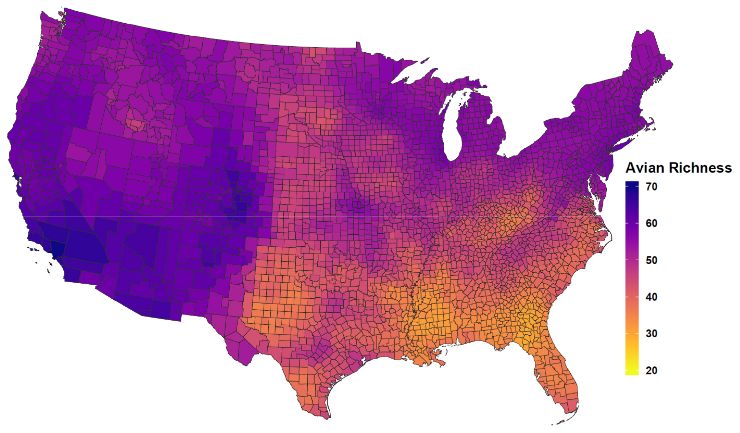
| Competent Host Richness | −0.03 | 0.01 | −0.04 | −0.02 |
| Max Temperature | 0.36 | 0.05 | 0.26 | 0.45 |
| Total Precipitation | 0.10 | 0.02 | 0.06 | 0.15 |
| WNV Mosquito Detection | 0.08 | 0.01 | 0.06 | 0.09 |
| WNV Avian Detection | 0.04 | 0.01 | 0.03 | 0.05 |
| AIANNH Population | −0.04 | 0.02 | −0.08 | −0.01 |
| AIANNH Lands | 0.05 | 0.02 | 0.02 | 0.09 |

References
- Beckham, J.D.; Tyler, K.L. Arbovirus Infections. Continuum 2015, 21, 1599–1611. [Google Scholar] [CrossRef] [Green Version]
- Lanciotti, R.S.; Roehrig, J.T.; Deubel, V.; Smith, J.; Parker, M.; Steele, K.; Crise, B.; Volpe, K.E.; Crabtree, M.B.; Scherret, J.H.; et al. Origin of the West Nile Virus Responsible for an Outbreak of Encephalitis in the Northeastern United States. Science 1999, 286, 2333–2337. [Google Scholar] [CrossRef] [Green Version]
- Kramer, L.D.; Ciota, A.T.; Marm Kilpatrick, A. Introduction, Spread, and Establishment of West Nile Virus in the Americas. J. Med. Entomol. 2019, 56, 1448–1455. [Google Scholar] [CrossRef] [PubMed]
- Centers for Disease Control and Prevention. ArboNET. Available online: https://wwwn.cdc.gov/arbonet (accessed on 21 August 2019).
- Centers for Disease Control and Prevention. CDC 2015 Case Definition. Available online: https://wwwn.cdc.gov/nndss/conditions/arboviral-diseases-neuroinvasive-and-non-neuroinvasive/case-definition/2015/ (accessed on 1 April 2021).
- Busch, M.P.; Wright, D.J.; Custer, B.; Tobler, L.H.; Stramer, S.L.; Kleinman, S.H.; Prince, H.E.; Bianco, C.; Foster, G.; Petersen, L.R.; et al. West Nile virus infections projected from blood donor screening data, United States, 2003. Emerg. Infect. Dis. 2006, 12, 395–402. [Google Scholar] [CrossRef] [PubMed]
- Carson, P.J.; Borchardt, S.M.; Custer, B.; Prince, H.E.; Dunn-Williams, J.; Winkelman, V.; Tobler, L.; Biggerstaff, B.J.; Lanciotti, R.; Petersen, L.R.; et al. Neuroinvasive disease and West Nile virus infection, North Dakota, USA, 1999–2008. Emerg. Infect. Dis. 2012, 18, 684–686. [Google Scholar] [CrossRef] [PubMed]
- Petersen, L.R. Epidemiology of West Nile Virus in the United States: Implications for Arbovirology and Public Health. J. Med. Entomol. 2019, 56, 1456–1462. [Google Scholar] [CrossRef] [PubMed] [Green Version]
- Weber, I.B.; Lindsey, N.P.; Bunko-Patterson, A.M.; Briggs, G.; Wadleigh, T.J.; Sylvestor, T.L.; Levy, C.; Komatsu, K.K.; Lehman, J.A.; Fischer, M.; et al. Completeness of West Nile virus testing in patients with meningitis and encephalitis during an outbreak in Arizona, USA. Epidemiol. Infect. 2012, 140, 1632–1636. [Google Scholar] [CrossRef]
- Ciota, A.T. West Nile virus and its vectors. Curr. Opin. Insect Sci. 2017, 22, 28–36. [Google Scholar] [CrossRef]
- Reisen, W.K. Landscape Epidemiology of Vector-Borne Diseases. Annu. Rev. Entomol. 2010, 55, 461–483. [Google Scholar] [CrossRef] [Green Version]
- Ruiz, M.O.; Chaves, L.F.; Hamer, G.L.; Sun, T.; Brown, W.M.; Walker, E.D.; Haramis, L.; Goldberg, T.L.; Kitron, U.D. Local impact of temperature and precipitation on West Nile virus infection in Culex species mosquitoes in northeast Illinois, USA. Parasites Vectors 2010, 3, 1–16. [Google Scholar] [CrossRef] [Green Version]
- Paull, S.H.; Kilpatrick, A.M.; Horton, D.E.; Diffenbaugh, N.S.; Ashfaq, M.; Rastogi, D.; Kramer, L.D. Drought and immunity determine the intensity of west nile virus epidemics and climate change impacts. Proc. R. Soc. B Biol. Sci. 2017, 284. [Google Scholar] [CrossRef] [PubMed]
- Tolsá, M.J.; García-Peña, G.E.; Rico-Chávez, O.; Roche, B.; Suzán, G. Macroecology of birds potentially susceptible to West Nile virus. Proc. R. Soc. B Biol. Sci. 2018, 285. [Google Scholar] [CrossRef] [PubMed] [Green Version]
- Hahn, M.B.; Monaghan, A.J.; Hayden, M.H.; Eisen, R.J.; Delorey, M.J.; Lindsey, N.P.; Nasci, R.S.; Fischer, M. Meteorological conditions associated with increased incidence of west nile virus disease in the United States, 2004–2012. Am. J. Trop. Med. Hyg. 2015. [Google Scholar] [CrossRef] [PubMed]
- McDonald, E.; Martin, S.W.; Landry, K.; Gould, C.V.; Lehman, J.; Fischer, M.; Lindsey, N.P. West Nile virus and other domestic nationally notifiable arboviral diseases—United States, 2018. Am. J. Transplant. 2019, 19, 2949–2954. [Google Scholar] [CrossRef] [Green Version]
- Lindsey, N.P.; Staples, J.E.; Lehman, J.A.; Fischer, M. Medical Risk Factors for Severe West Nile Virus Disease, United States, 2008–2010. Am. Soc. Trop. Med. Hyg. 2012, 87, 179–184. [Google Scholar] [CrossRef] [Green Version]
- Perez, A.M.; Thurmond, M.C.; Carpenter, T.E. Spatial distribution of foot-and-mouth disease in Pakistan estimated using imperfect data. Prev. Vet. Med. 2006, 76, 280–289. [Google Scholar] [CrossRef] [PubMed]
- Beasley, D.W. Vaccines and immunotherapeutics for the prevention and treatment of infections with West Nile virus. Immunotherapy 2011, 3, 269–285. [Google Scholar] [CrossRef]
- LaDeau, S.L.; Glass, G.E.; Hobbs, N.T.; Latimer, A.; Ostfeld, R.S. Data-model fusion to better understand emerging pathogens and improve infectious disease forecasting. Ecol. Appl. 2011, 21, 1443–1460. [Google Scholar] [CrossRef] [PubMed]
- Niu, S.; Luo, Y.; Dietze, M.C.; Keenan, T.F.; Shi, Z.; Li, J.; Chapin, F.S. The role of data assimilation in predictive ecology. Ecosphere 2014, 5, 1–16. [Google Scholar] [CrossRef]
- Peters, D.P.; McVey, D.S.; Elias, E.H.; Pelzel-McCluskey, A.M.; Derner, J.D.; Burruss, N.D.; Schrader, T.S.; Yao, J.; Pauszek, S.J.; Lombard, J.; et al. Big data–model integration and AI for vector-borne disease prediction. Ecosphere 2020, 11. [Google Scholar] [CrossRef]
- Hartley, D.M.; Barker, C.M.; Le Menach, A.; Niu, T.; Gaff, H.D.; Reisen, W.K. Effects of Temperature on Emergence and Seasonality of West Nile Virus in California. Am. J. Trop. Med. Hyg. 2012, 86, 884–894. [Google Scholar] [CrossRef] [PubMed] [Green Version]
- Ukawuba, I.; Shaman, J. Association of spring-summer hydrology and meteorology with human West Nile virus infection in West Texas, USA, 2002–2016. Parasites Vectors 2018, 11, 1–15. [Google Scholar] [CrossRef] [PubMed]
- Bureau, C. Small Area Income and Poverty Estimates (SAIPE) Program. 2018. Available online: https://www.census.gov/programs-surveys/saipe.html (accessed on 15 July 2019).
- Wey, C.L.; Griesse, J.; Kightlinger, L.; Wimberly, M.C. Geographic variability in geocoding success for West Nile virus cases in South Dakota. Health Place 2009, 15, 1108–1114. [Google Scholar] [CrossRef] [PubMed] [Green Version]
- Yellow Horse, A.J.; Yang, T.C.; Huyser, K.R. Structural Inequalities Established the Architecture for COVID-19 Pandemic Among Native Americans in Arizona: A Geographically Weighted Regression Perspective. J. Racial Ethn. Health Disparities 2021. [Google Scholar] [CrossRef]
- Sullivan, B.L.; Aycrigg, J.L.; Barry, J.H.; Bonney, R.E.; Bruns, N.; Cooper, C.B.; Damoulas, T.; Dhondt, A.A.; Dietterich, T.; Farnsworth, A.; et al. The eBird enterprise: An integrated approach to development and application of citizen science. Biol. Conserv. 2014, 169, 31–40. [Google Scholar] [CrossRef]
- PRISM. Total Annual Precipitation and Mean Maximum Temperature Climate Data. Available online: http://prism.oregonstate.edu (accessed on 12 June 2020).
- Wearing, H.J.; Rohani, P. Ecological and immunological determinants of dengue epidemics. Proc. Natl. Acad. Sci. USA 2006, 103, 11802–11807. [Google Scholar] [CrossRef] [Green Version]
- Johansson, M.A.; Hombach, J.; Cummings, D.A.T. Models of the impact of dengue vaccines: A review of current research and potential approaches. Vaccine 2011, 29, 5860–5868. [Google Scholar] [CrossRef] [PubMed] [Green Version]
- Johansson, M.A.; Reich, N.G.; Hota, A.; Brownstein, J.S.; Santillana, M. Evaluating the performance of infectious disease forecasts: A comparison of climate-driven and seasonal dengue forecasts for Mexico. Sci. Rep. 2016, 6, 33707. [Google Scholar] [CrossRef] [Green Version]
- Grenfell, B.T.; Anderson, R.M. The estimation of age-related rates of infection from case notifications and serological data. J. Hyg. 1985, 95, 419–436. [Google Scholar] [CrossRef] [PubMed]
- Medone, P.; Ceccarelli, S.; Parham, P.E.; Figuera, A.; Rabinovich, J.E. The impact of climate change on the geographical distribution of two vectors of chagas disease: Implications for the force of infection. Philos. Trans. R. Soc. Biol. Sci. 2015, 370, 1–12. [Google Scholar] [CrossRef] [Green Version]
- Manrique, P.D.; Xu, C.; Hui, P.M.; Johnson, N.F. Atypical viral dynamics from transport through popular places. Phys. Rev. E 2016, 94, 022304. [Google Scholar] [CrossRef] [PubMed] [Green Version]
- Sallam, M.F.; Fizer, C.; Pilant, A.N.; Whung, P.Y. Systematic review: Land cover, meteorological, and socioeconomic determinants of aedes mosquito habitat for risk mapping. Int. J. Environ. Res. Public Health 2017, 14, 1230. [Google Scholar] [CrossRef] [PubMed] [Green Version]
- Massad, E.; Tan, S.H.; Khan, K.; Wilder-Smith, A. Estimated Zika virus importations to Europe by travellers from Brazil. Glob. Health Action 2016, 9. [Google Scholar] [CrossRef] [PubMed]
- Field, R.; Hawkins, B.A.; Cornell, H.V.; Currie, D.J.; Diniz-Filho, J.A.F.; Guégan, J.F.; Kaufman, D.M.; Kerr, J.T.; Mittelbach, G.G.; Oberdorff, T.; et al. Spatial species-richness gradients across scales: A meta-analysis. J. Biogeogr. 2009, 36, 132–147. [Google Scholar] [CrossRef]
- Elsner, J.B.; Fricker, T.; Widen, H.M.; Castillo, C.M.; Humphreys, J.; Jung, J.; Rahman, S.; Richard, A.; Jagger, T.H.; Bhatrasataponkul, T.; et al. The relationship between elevation roughness and tornado activity: A spatial statistical model fit to data from the central great plains. J. Appl. Meteorol. Climatol. 2016, 55, 849–859. [Google Scholar] [CrossRef]
- Humphreys, J.M.; Murrow, J.L.; Sullivan, J.D.; Prosser, D.J. Seasonal occurrence and abundance of dabbling ducks across the continental United States: Joint spatio-temporal modelling for the Genus Anas. Divers. Distrib. 2019, 25, 1497–1508. [Google Scholar] [CrossRef] [Green Version]
- Humphreys, J.M.; Ramey, A.M.; Douglas, D.C.; Mullinax, J.M.; Soos, C.; Link, P.; Walther, P.; Prosser, D.J. Waterfowl occurrence and residence time as indicators of H5 and H7 avian influenza in North American Poultry. Sci. Rep. 2020, 10, 2592. [Google Scholar] [CrossRef] [PubMed]
- Belsley, D.A.; Kuh, E.; Welsch, R.E. Regression Diagnostics: Identifying Influential Data and Sources of Collinearit; John Wiley: Hoboken, NJ, USA, 1980; pp. 85–115. [Google Scholar]
- Hendricks, J.; Pelzer, B. Collinearity involving ordered and unordered categorical variables. Presented at the RC33 Conference, Amsterdam, The Netherlands, 17–20 August 2004. [Google Scholar]
- Bernardinelli, L.; Pascutto, C.; Best, N.G.; Gilks, W.R. Disease mapping with errors in covariates. Stat. Med. 1997, 16, 741–752. [Google Scholar] [CrossRef]
- Ancelet, S.; Abellan, J.J.; Del Rio Vilas, V.J.; Birch, C.; Richardson, S. Bayesian shared spatial-component models to combine and borrow strength across sparse disease surveillance sources. Biom. J. 2012, 54, 385–404. [Google Scholar] [CrossRef]
- Jaya, I.G.N.M.; Folmer, H. Bayesian Spatiotemporal Mapping of Relative Dengue Disease Risk in Bandung, Indonesia; Springer: Berlin/Heidelberg, Germany, 2020; Volume 22, pp. 105–142. [Google Scholar] [CrossRef]
- Elliott, P.; Wakefield, J.; Best, N.; Briggs, D. Spatial Epidemiology: Methods and Applications; Oxford University Press: Oxford, UK, 2000. [Google Scholar]
- Lawson, A.B. Bayesian Disease Mapping: Hierarchical Modeling in Spatial Epidemiology, 3rd ed.; Chapman and Hall/CRC Press: Boca Raton, FL, USA, 2018. [Google Scholar]
- Dean, C.B.; Ugarte, M.D.; Militino, A.F. Detecting interaction between random region and fixed age effects in disease mapping. Biometrics 2001, 57, 197–202. [Google Scholar] [CrossRef] [PubMed]
- Simpson, D.; Rue, H.; Riebler, A.; Martins, T.G.; Sørbye, S.H. Penalising Model Component Complexity: A Principled, Practical Approach to Constructing Priors. Stat. Sci. 2017, 32, 1–28. [Google Scholar] [CrossRef]
- Besag, J.; York, J.; Mollié, A. Bayesian image restoration, with two applications in spatial statistics. Ann. Inst. Stat. Math. 1991, 43, 1–20. [Google Scholar] [CrossRef]
- Breslow, N.; Leroux, B.; Platt, R. Approximate hierarchical modelling of discrete data in epidemiology. Stat. Methods Med. Res. 1998, 7, 49–62. [Google Scholar] [CrossRef]
- Riebler, A.; Sørbye, S.H.; Simpson, D.; Rue, H.; Lawson, A.B.; Lee, D.; MacNab, Y. An intuitive Bayesian spatial model for disease mapping that accounts for scaling. Stat. Methods Med. Res. 2016, 25, 1145–1165. [Google Scholar] [CrossRef] [PubMed] [Green Version]
- Bivand, R.; Piras, G. Comparing Implementations of Estimation Methods for Spatial Econometrics. J. Stat. Softw. 2015, 63. [Google Scholar] [CrossRef] [Green Version]
- Rue, H.; Martino, S.; Chopin, N. Approximate Bayesian inference for latent Gaussian models by using integrated nested Laplace approximations. J. R. Stat. Soc. Ser. Stat. Methodol. 2009, 71, 319–392. [Google Scholar] [CrossRef]
- Martins, T.G.; Simpson, D.; Lindgren, F.; Rue, H. Bayesian computing with INLA: New features. Comput. Stat. Data Anal. 2013, 67, 68–83. [Google Scholar] [CrossRef] [Green Version]
- Lindgren, F.; Rue, H. Bayesian Spatial Modelling with R-INLA. J. Stat. Softw. 2015, 63, 1–25. [Google Scholar] [CrossRef] [Green Version]
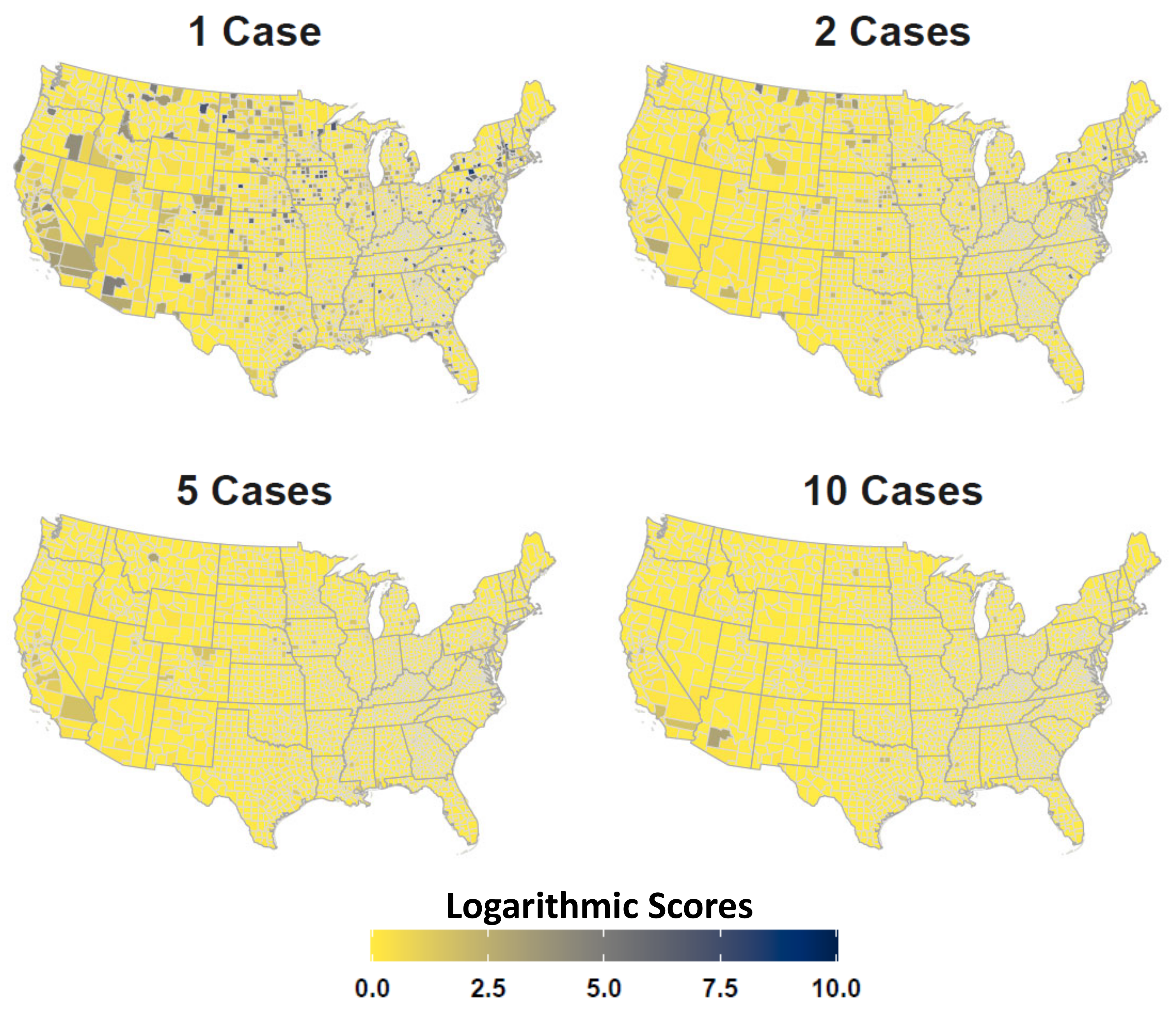
- Gneiting, T.; Raftery, A.E. Strictly Proper Scoring Rules, Prediction, and Estimation. J. Am. Stat. Assoc. 2007, 102, 359–378. [Google Scholar] [CrossRef]
- Brier, G.W. Verification of forecasts expressed in terms of probability. Mon. Weather Rev. 1950, 78, 1–3. [Google Scholar] [CrossRef]
- ECOMAP. National Hierarchical Framework of Ecological Units. USDA Forest Service; Yale University Press: New Haven, CT, USA, 1993. [Google Scholar]
- Barker, C.M.; Bolling, B.G.; Black, W.C., IV; Moore, C.G.; Eisen, L. Mosquitoes and West Nile virus along a river corridor from prairie to montane habitats in eastern Colorado. J. Vector Ecol. 2009, 34, 276–293. [Google Scholar] [CrossRef] [PubMed]
- Chuang, T.W.; Hildreth, M.B.; Vanroekel, D.L.; Wimberly, M.C. Weather and Land Cover Influences on Mosquito Populations in Sioux Falls, South Dakota. J. Med. Entomol. 2011, 48, 669–679. [Google Scholar] [CrossRef] [PubMed] [Green Version]
- Avise, J.C. Phylogeography: Retrospect and prospect. J. Biogeogr. 2009, 36, 3–15. [Google Scholar] [CrossRef] [Green Version]
- Oomen, R.A.; Reudink, M.W.; Nocera, J.J.; Somers, C.M.; Green, M.C.; Kyle, C.J. Mitochondrial Evidence for Panmixia despite Perceived Barriers to Gene Flow in a Widely Distributed Waterbird. J. Hered. 2011, 102, 584–592. [Google Scholar] [CrossRef] [PubMed] [Green Version]
- Ruegg, K.C.; Smith, T.B. Not as the Crow Flies: A Historical Explanation for Circuitous Migration in Swainson’s Thrush (Catharus ustulatus). Proc. Biol. Sci. 2002, 269, 1375–1381. [Google Scholar] [CrossRef] [PubMed] [Green Version]
- Kelly, J.F.; Hutto, R.L. An East–West Comparison of Migration in North American Wood Warblers. Condor 2005, 107, 197–211. [Google Scholar] [CrossRef]
- Landesman, W.J.; Allan, B.F.; Langerhans, R.B.; Knight, T.M.; Chase, J.M. Inter-Annual Associations Between Precipitation and Human Incidence of West Nile Virus in the United States. Vector-Borne Zoonotic Dis. 2007, 7, 337–343. [Google Scholar] [CrossRef]
- Benedum, C.M.; Seidahmed, O.M.E.; Eltahir, E.A.B.; Markuzon, N. Statistical modeling of the effect of rainfall flushing on dengue transmission in Singapore. PLoS Neglected Trop. Dis. 2018, 12, 1–18. [Google Scholar] [CrossRef]
- Hawley, W.A.; Pumpuni, C.B.; Brady, R.H.; Craig, G.B.J. Overwintering Survival of Aedes albopictus (Diptera: Culicidae) Eggs in Indiana. J. Med. Entomol. 1989, 26, 122–129. [Google Scholar] [CrossRef]
- Chuang, T.W.; Knepper, R.G.; Stanuszek, W.W.; Walker, E.D.; Wilson, M.L. Temporal and Spatial Patterns of West Nile Virus Transmission in Saginaw County, Michigan, 2003–2006. J. Med. Entomol. 2011, 48, 1047–1056. [Google Scholar] [CrossRef] [PubMed]
- Gardner, A.M.; Hamer, G.L.; Hines, A.M.; Newman, C.M.; Walker, E.D.; Ruiz, M.O. Weather Variability Affects Abundance of Larval Culex (Diptera: Culicidae) in Storm Water Catch Basins in Suburban Chicago. J. Med. Entomol. 2012, 49, 270–276. [Google Scholar] [CrossRef] [PubMed] [Green Version]
- Kwan, J.; Park, B.; Carpenter, T.; Ngo, V.; Civen, R.; Reisen, W. Comparison of enzootic risk measures for predicting West Nile disease, Los Angeles, California, USA, 2004–2010. Emerg. Infect. Dis. 2012, 18, 1298–1306. [Google Scholar] [CrossRef] [PubMed]
- Kovach, T.J.; Kilpatrick, A.M. Increased Human Incidence of West Nile Virus Disease near Rice Fields in California but Not in Southern United States. Am. J. Trop. Med. Hyg. 2018, 99, 222–228. [Google Scholar] [CrossRef] [PubMed]
- WNV Surveillance, Centers for Disease Control and Prevention. CDC. Available online: https://www.cdc.gov/westnile/index.html (accessed on 30 April 2021).
- Thiemann, T.C.; Wheeler, S.S.; Barker, C.M.; Reisen, W.K. Mosquito host selection varies seasonally with host availability and mosquito density. PLoS Neglected Trop. Dis. 2011, 5. [Google Scholar] [CrossRef]
- Ostfeld, R.S.; Keesing, F. Biodiversity and Disease Risk: The Case of Lyme Disease. Conserv. Biol. 2000, 14, 722–728. [Google Scholar] [CrossRef]
- Marini, G.; Rosá, R.; Pugliese, A.; Heesterbeek, H. Exploring vector-borne infection ecology in multi-host communities: A case study of West Nile virus. J. Theor. Biol. 2017, 415, 58–69. [Google Scholar] [CrossRef] [Green Version]
- Simpson, J.E.; Hurtado, P.J.; Medlock, J.; Molaei, G.; Andreadis, T.G.; Galvani, A.P.; Diuk-Wasser, M.A. Vector host-feeding preferences drive transmission of multi-host pathogens: West Nile virus as a model system. Proc. R. Soc. B Biol. Sci. 2012, 279, 925–933. [Google Scholar] [CrossRef] [Green Version]
- Hamer, G.L.; Chaves, L.F.; Anderson, T.K.; Kitron, U.D.; Brawn, J.D.; Ruiz, M.O.; Loss, S.R.; Walker, E.D.; Goldberg, T.L. Fine-scale variation in vector host use and force of infection drive localized patterns of West Nile virus transmission. PLoS ONE 2011, 6. [Google Scholar] [CrossRef] [Green Version]
- Both, C.; Bouwhuis, S.; Lessells, C.; Visser, M.E. Climate change and population declines in a long-distance migratory bird. Nature 2006, 441, 81–83. [Google Scholar] [CrossRef] [Green Version]
- Marra, P.P.; Francis, C.M.; Mulvihill, R.S.; Moore, F.R. The influence of climate on the timing and rate of spring bird migration. Oecologia 2005, 142, 307–315. [Google Scholar] [CrossRef] [PubMed]
- Rohani, P.; Earn, D.J.D.; Grenfell, B.T. Opposite Patterns of Synchrony in Sympatric Disease Metapopulations. Science 1999, 286, 968–971. [Google Scholar] [CrossRef] [PubMed]
- Baquero, O.S.; Machado, G. Spatiotemporal dynamics and risk factors for human Leptospirosis in Brazil. Sci. Rep. 2018, 8, 15170. [Google Scholar] [CrossRef] [PubMed] [Green Version]
- Humphreys, J.M.; Elsner, J.B.; Jagger, T.H.; Pau, S. A Bayesian geostatistical approach to modeling global distributions of Lygodium microphyllum under projected climate warming. Ecol. Model. 2017, 363, 192–206. [Google Scholar] [CrossRef]


| Model | DIC | WAIC | Description |
|---|---|---|---|
| Model1 | 65491 | 65690 | Non-spatiotemporal (All fixed covariates) |
| Model2 | 40699 | 40355 | Spatiotemporal (No fixed covariates) |
| Model3 | 40281 | 39798 | Individual Neuroinvasive (All covariates) |
| Model4 | 55937 | 55889 | Joint Disease (No fixed effects) |
| Model5 | 38680 | 38082 | Full Joint Disease (All covariates) |
| Covariate | Mean | SD | 2.5 Q | 97.5 Q |
|---|---|---|---|---|
| Intercept | −0.54 | 0.17 | −0.86 | −0.22 |
| Median Household Income | −0.08 | 0.02 | −0.12 | −0.04 |
| Historic Prevalence | −0.09 | 0.02 | −0.12 | −0.05 |
| Proportion Years | 1.40 | 0.08 | 1.25 | 1.55 |
| County Geographic Area | 0.71 | 0.27 | 0.18 | 1.24 |
| Competent Host Richness | −0.05 | 0.01 | −0.06 | −0.05 |
| Max Temperature | 0.16 | 0.04 | 0.09 | 0.23 |
| Total Precipitation | 0.03 | 0.02 | −0.01 | 0.07 |
| WNV Mosquito Detection | 0.04 | 0.01 | 0.04 | 0.05 |
| WNV Avian Detection | 0.03 | 0.01 | 0.02 | 0.04 |
| AIANNH Population | −0.04 | 0.01 | −0.06 | −0.01 |
| AIANNH Lands | 0.07 | 0.01 | 0.04 | 0.09 |
| Disease Interaction () | 0.89 | 0.20 | 0.84 | 0.92 |
Publisher’s Note: MDPI stays neutral with regard to jurisdictional claims in published maps and institutional affiliations. |
© 2021 by the authors. Licensee MDPI, Basel, Switzerland. This article is an open access article distributed under the terms and conditions of the Creative Commons Attribution (CC BY) license (https://creativecommons.org/licenses/by/4.0/).
Share and Cite
Humphreys, J.M.; Young, K.I.; Cohnstaedt, L.W.; Hanley, K.A.; Peters, D.P.C. Vector Surveillance, Host Species Richness, and Demographic Factors as West Nile Disease Risk Indicators. Viruses 2021, 13, 934. https://0-doi-org.brum.beds.ac.uk/10.3390/v13050934
Humphreys JM, Young KI, Cohnstaedt LW, Hanley KA, Peters DPC. Vector Surveillance, Host Species Richness, and Demographic Factors as West Nile Disease Risk Indicators. Viruses. 2021; 13(5):934. https://0-doi-org.brum.beds.ac.uk/10.3390/v13050934
Chicago/Turabian StyleHumphreys, John M., Katherine I. Young, Lee W. Cohnstaedt, Kathryn A. Hanley, and Debra P. C. Peters. 2021. "Vector Surveillance, Host Species Richness, and Demographic Factors as West Nile Disease Risk Indicators" Viruses 13, no. 5: 934. https://0-doi-org.brum.beds.ac.uk/10.3390/v13050934