
Collaborative Filtering Based on a Variational Gaussian Mixture Model


School of Computer Engineering and Science, Shanghai University, Shanghai 200444, China
*
Author to whom correspondence should be addressed.
Future Internet 2021, 13(2), 37; https://0-doi-org.brum.beds.ac.uk/10.3390/fi13020037
Submission received: 18 December 2020
/
Revised: 28 January 2021
/
Accepted: 28 January 2021
/
Published: 1 February 2021
(This article belongs to the Collection Computer Vision, Deep Learning and Machine Learning with Applications)
Abstract
:Collaborative filtering (CF) is a widely used method in recommendation systems. Linear models are still the mainstream of collaborative filtering research methods, but non-linear probabilistic models are beyond the limit of linear model capacity. For example, variational autoencoders (VAEs) have been extensively used in CF, and have achieved excellent results. Aiming at the problem of the prior distribution for the latent codes of VAEs in traditional CF is too simple, which makes the implicit variable representations of users and items too poor. This paper proposes a variational autoencoder that uses a Gaussian mixture model for latent factors distribution for CF, GVAE-CF. On this basis, an optimization function suitable for GVAE-CF is proposed. In our experimental evaluation, we show that the recommendation performance of GVAE-CF outperforms the previously proposed VAE-based models on several popular benchmark datasets in terms of recall and normalized discounted cumulative gain (NDCG), thus proving the effectiveness of the algorithm.
1. Introduction
Today, recommendation systems are extensively used in business and scientific research to help users mine valuable information from massive amounts of data. The data required by the recommendation systems are sourced from user clicks, comments, purchases, searches, and other records. The behavior habits and preferences of users are explored to analyze the items that they are most likely to consume, as well as to ultimately help users find their needs more efficiently [1].
Currently, the mainstream recommendation algorithms are collaborative filtering (CF) algorithms, which establish the preference prediction model by exploring the similarity pattern of users and items. Generally speaking, there are three methods of CF: The content-based recommendation algorithm [2,3], the CF recommendation algorithm, and the hybrid recommendation algorithm. The Content-based recommendation algorithm mainly uses the information of users and items to predict users’ preferences. With the continuous development of society, people pay more and more attention to their privacy, which makes it more difficult to collect users’ information. Therefore, the content-based recommendation algorithm has gradually failed to meet the needs of users. Meanwhile, the CF recommendation algorithm is divided into memory-based CF [4] and model-based CF. Memory-based CF can be further divided into user-based [5] and item-based [6] methods. Memory-based methods use the data of the relationship between users or items to recommend items to users that they have never seen before. While model-based methods are principal methods of recommendation algorithms [7,8]. They learn a model through the historical behavior data of users to predict the users preferences. These model can use machine learning algorithms. For example, matrix factorization (MF) is one of the most popular methods in the industry. Severinski et al. [9] add constraints of Gibbs updates for the side features vector of probabilistic matrix factorization (PMF), and this Bayesian constrained PMF model is superior to simple MAP estimation.
However, MF cannot capture the non-linearity relationships between users and items. To tackle this problem, the generative models have attracted the attention of researchers. The first generative model that appeared in the literature of recommendation systems was the generative adversarial network (GAN) [10,11]. Immediately afterwards, a series of variational autoencoders (VAEs) also appeared, and they achieved better results than using GAN for recommendation systems [12,13]. Liang et al. [14] used VAEs for the first time to conduct CF by extending VAEs to CF recommendation algorithms for implicit feedback, which made up for the shortcomings of less research on non-linear models in recommendation systems. Kim et al. [15] modified the distribution of the latent factors in the original VAE and used a flexible prior distribution, and said that this method can better represent the user preferences. Shenbin et al. [16] introduced a recommender VAE (RecVAE) model that uses a novel composite prior distribution for the latent representation. The distribution of the hidden variables of the VAE model in the above CF algorithm is too simple, and it cannot effectively learn the complex non-linear relationships between users and items. In summary, our contributions are as follows:
- We propose a new variational autoencoder CF model (i.e., a Gaussian mixture model for latent factor distribution for CF (GVAE-CF)). Specifically, we change the single Gaussian posterior distribution in the standard variational autoencoder to a Gaussian mixture model (GMM), and we propose a GMM-based variational autoencoder neural network structure for CF. The model can effectively learn the relationships of users and items.
- We re-derive the variational lower bound of the variational autoencoder.
- We compare the latent space representations of the standard VAE and GVAE-CF to study the GVAE-CF internal mechanism of the GVAE-CF.
2. Background and Related Work
At present, deep learning is achieving great success in many fields, with many researchers paying attention to this area. Because of the powerful ability of the neural network to discover the non-linear relationships in a complex dataset of recommendation systems, researchers have begun to utilize the neural network to address the problem of CF. MF is the most successful technique among the model-based methods [12,13,17]. Billsus et al. [18] used singular value decomposition (SVD) to conduct CF, which is the earliest CF model based on the MF algorithm. Mnih et al. [13] proposed a probabilistic linear model with Gaussian noise, called the PMF. Alquier et al. [19] introduced a standard way to assign an inverse gamma prior to the singular values of a certain SVD of the matrix of interest. The experimental results showed that the performance of the PMF is better than that of SVD. Alexandridis et al. [20] tried to combine the advantages of some previous methods, such as soft-clustering on user’s social networks. However, the above models are linear models, and they cannot capture the complex relationships between users and items. Liang et al. [21] proved that adding non-linear features to the hidden linear factor model can effectively improve the performance of the recommendation systems.
Due to the powerful ability of generative models to fit non-linear and uncertain data, they have become a very popular choice for CF algorithms. Lee et al. [22] proposed an enhanced VAE to improve recommendation performance through adding auxiliary information input. Liang et al. [14] proposed a model-based CF algorithm called Mult-VAE, which takes user-item binary score data as the input and learns a compressed latent representations. The latent factors are then used to reconstruct the input vector and to calculate the missing score. Different from the standard VAE, Mult-VAE adopts multinomial likelihood instead of Gaussian likelihood. They authors claim that the polynomial distribution is more suitable for the recommendation systems. Shenbin et al. [16] modified the distribution of the hidden factors in the standard VAE and adopted a compound prior method combining a standard Gaussian distribution and a potential code distribution. Askari et al. [23] utilized two VAEs to form a compound VAE, which can learn the relationships between users and items at the same time.
Compared to the previous methods, in this paper, we overcome the shortcoming of VAEs using very simple posterior distribution to learn latent codes between users and items. In the current CF, the Gaussian distribution is used, which allows our model to fit some extremely distorted multi-peak distributions.
3. Method
In this section, we introduce a VAE for the CF algorithm that uses a GMM for the prior distribution of latent factors, abbreviated as GVAE-CF. First, we briefly introduce VAE, for which further details can be read in References [24,25].
3.1. Variational Autoencoder
A variational autoencoder is a generative model, whose purposed is to discover the principle of data generation in the form of probability distribution. For each user u, the model samples an M-dimensional latent factor z from a standard Gaussian prior distribution. It is assumed that the input x is generated by the following process:
where z is a latent factor that cannot be observed, and the dimension is lower than the dimension of the input x. The goal of VAE is to maximize the log likelihood (maximum likelihood estimation (MLE)) of the data to estimate the parameter . The MLE is calculated through:
Equation (2) needs to calculate all latent representations, which is a problem that cannot be solved directly. To make this problem tractable, we usually use a posterior distribution to approximate the true posterior , where is a parameter. In traditional variational autoencoders, we usually use a standard Gaussian distribution, and the similarity between and the posterior distribution is measured by minimizing the Kullback-Liebler(KL) divergence. Since the marginal likelihood function is difficult to obtain, it is usually obtained approximately via the evidence lower bound (ELBO):
where denotes the expectation. The first term of the reconstruction error is to reduce the distance between the input x and the reconstruction , while the second term is the KL divergence between the variational posterior and the standard Gaussian distribution . It should be noted that , embeds the input x into a low-dimensional manifold.
In fact, and determine the parameters through two deep neural networks, corresponding to the encoder and decoder , respectively. These parameters are optimized using stochastic gradient algorithms with the help of a reparameterization trick [26,27]. Finally, the encoder network determines the parameters, such as mean and variance , by defining the distribution of each data point z. Since the sampling operation is non-differentiable, it is transformed as follows:
where is sampled from the standard normal distribution. Since only linear transformation is involved, the stochastic gradient algorithm can be used to update the parameters.
3.2. Variational Autoencoder Based on the GMM for CF
In this part, we modified the prior distribution of the latent factors of the standard VAE into a Gaussian mixture model, and we propose a GVAE-CF algorithm for the CF problem. We show the difference between GVAE-CF and the most advanced algorithms, and then we define the model structure and a novel loss function.
First of all, we briefly introduce the Gaussian mixture model. The mathematical form of Gaussian mixture is as follows:
where is the standard Gaussian model with mean and covariance matrix , is the weight coefficient of the i-th standard Gaussian model, and , , k is the number of single Gaussian models. For each user u, we need to learn approximately the computable posterior distribution . Variational inference simply uses a variational distribution as the approximate uncalculated posterior. Here, we set to be k completely diagonal Gaussian distributions. Therefore, the covariance matrix can be represented by the vector .
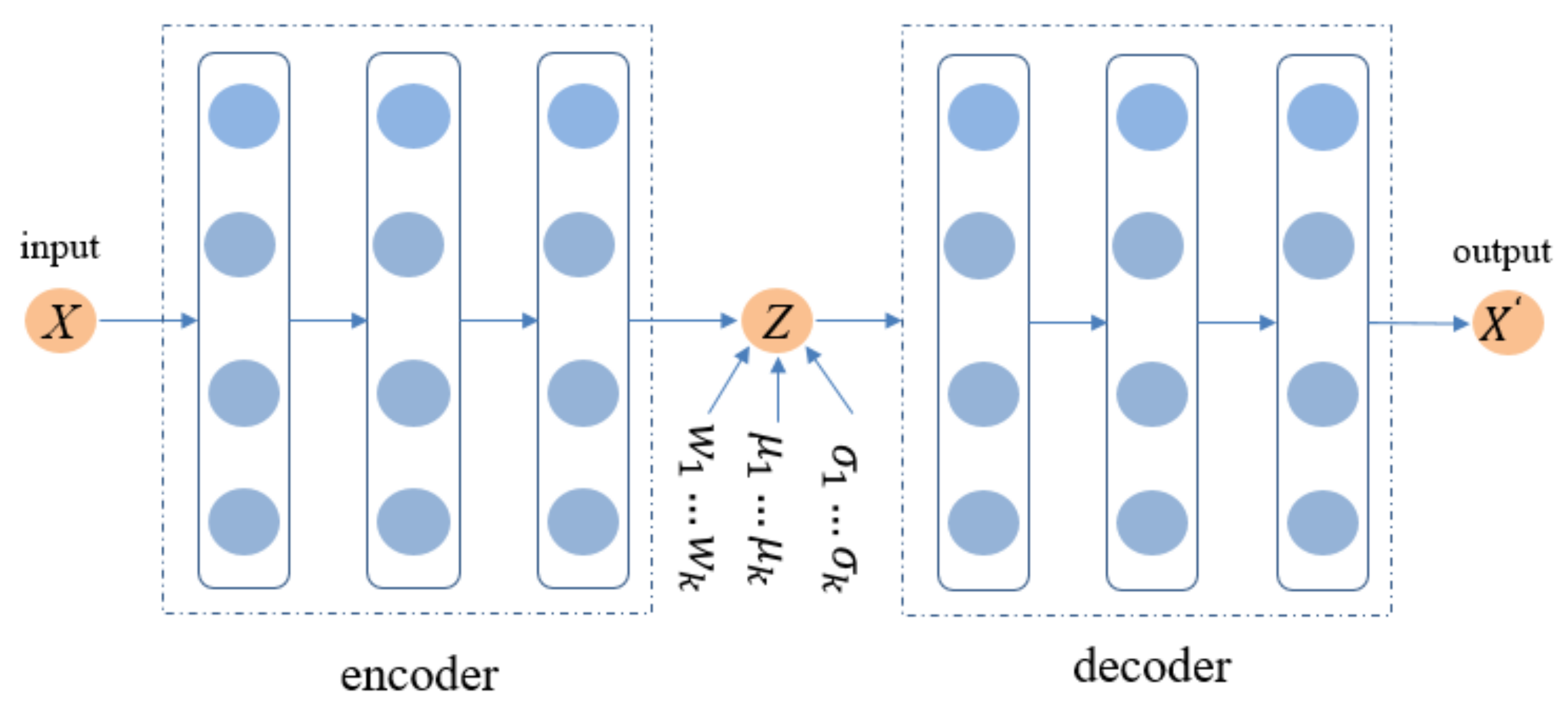
Similar to the standard variational autoencoder, GVAE-CF is also represented as a latent factor model. The most critical difference lies in the structural changes brought about by the distribution of the latent factors. As shown in Figure 1, a vector is used as the input, and it is mapped to a hidden layer through the following functions:
Included are the mean vector , the variance vector , and the coefficient vector , among which refers to the diagonal matrices, which can be represented by vectors. The latent variable z adopts the reparameterization trick:
The sampling process of is: . Here, is a vector, and ⊙ means the dot product between two vectors.
Learning the GVAE-CF latent factor algorithm is similar to the standard variational inference [25]. The reconstruction error term in Equation (2) is not a required change. As we needed to modify the corresponding KL divergence loss. We tried:
where M is the dimension of the latent space, e is Euler number, and C is a larger constant set to prevent the gradient from disappearing. When calculating , in order to simplify the model and to facilitate the calculation, we can consider the spherical distribution we use, that is, the diagonal matrix of the covariance matrix, so can be simplified as:
As per the standard VAE, both estimate the parameters and . We can learn the unbiased estimation of ELBO by sampling , and can update and optimize the parameters through the stochastic gradient descent algorithm. However, the process of sampling is non-differentiable. Here, we used the reparameterization trick to avoid this problem [26,27]. Therefore, the z is sampled so that parameter can be back propagated. The training process of GVAE-CF is shown in Algorithm 1.
| Algorithm 1 GVAE-CF uses stochastic gradient descent algorithm to optimize the parameters |
Input: Rating matrix
|
4. Results
4.1. Datasets
This paper used three real-world datasets: MoviesLens-20M [28], Netflix [29], and LASTFM-2k. MoviesLens-20M contains 72,000 users rating for 10,000 movies, with a total of 10 million ratings and 100,000 tags. Netflix contains 480,189 users and 17,770 movie ratings. LASTFM-2k contains 1892 users and 92,800 songs recorded. For each dataset, we keep data with a score of 4 stars or more [30,31] and treated all other data as missing data. This approach has been widely used in previous recommendation systems [32,33,34]. This paper randomly used 80% of each data of user as the training set and the remaining 20% as the test set.
4.2. Metrics
In the top-R recommendation system, we recommended and predicted the R items with the highest ranking for each user. Following the experience of our predecessors, we employed two widely used evaluation indicators in the top-R recommendation system to evaluate the model: Recall@R and NDCG@R [35]. For GVAE-CF, we obtained the predicted R rankings by sorting the output of the decoder . Recall@R believes that ranking is just as important among R recommended items, but NDCG@R uses cumulative gains to make the higher ranked recommended items more important.
Recall: Given a top-R recommendation list based on the training set, represents the R recommendation lists selected by the user based on the test data. The recall rate of the entire recommendation system is calculated by calculating the average of the recall rate of each user. The recall rate is defined as:
Normalized discounted cumulative gain (NDCG): Among the recommended items, we paid more attention to the most relevant items at the top of the list. Therefore, we divided each term by an increasing number, also known as the loss value, to obtain the discounted cumulative gain (DCG). However, between users, the DCG is not directly comparable, so we have to normalize it. The worst situation is that the DCG is 0 when using non-negative correlation scores. To overcome this problem, we took the recommended items in the test set as the ideal recommendation order, obtained the top R items and calculated their DCG; this is called ideal DCG (IDCG). Finally, we divided the original DCG by the IDCG and obtained NDCG@R, which is a number between 0 and 1. Formally, we defined as the indicator function.
4.3. Experimental Setup
In order to train the model better, we divided all users into training/validation/test sets, where the number of validation set and test sets was the same. We used all of the historical click data of the training set to train the model. For evaluation, we used the validation set to adjust the hyperparameters of the model and to make a preliminary evaluation of the performance of the model. Following the practice of our predecessors, we sampled 80% of the rating data from each user in the remaining unobserved test set as the “fold-in” set to calculate the latent factors and to predict the remaining 20% of the rating data.
GVAE-CF uses the optimizer with a learning rate of and a batch size of 400. The encoder network consists of a fully connected neural network with 1200 neurons and a tanh as the activation function. Since the number of Gaussian components will affect the performance of the algorithm, this paper selected values from 2 to 32 in order to carry out the experiments and found that when the number of Gaussian components was 16, the model performed best on two indicators. Therefore, the output of the encoder was a Gaussian mixture model made up of 16 Gaussian components and then the hidden variables of 400 neurons obtained by sampling with the reparameterization trick. The decoder network was also composed of a fully connected neural network with 1200 neurons and a tanh as the activation function.
4.4. Latent Space Exploration
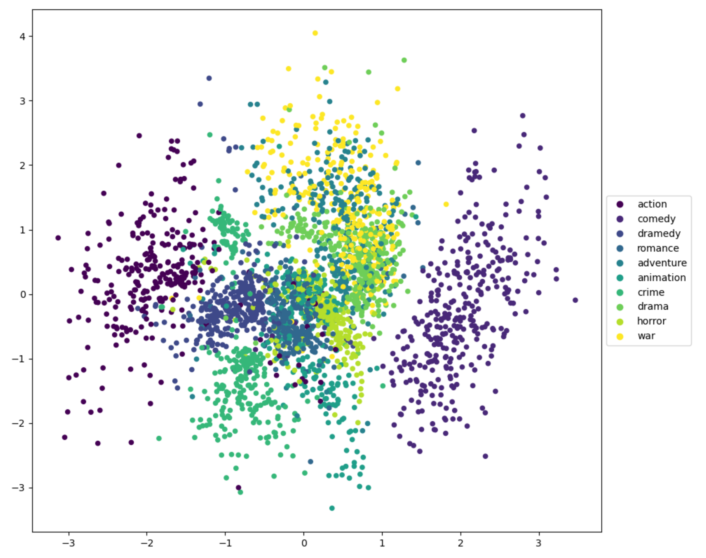
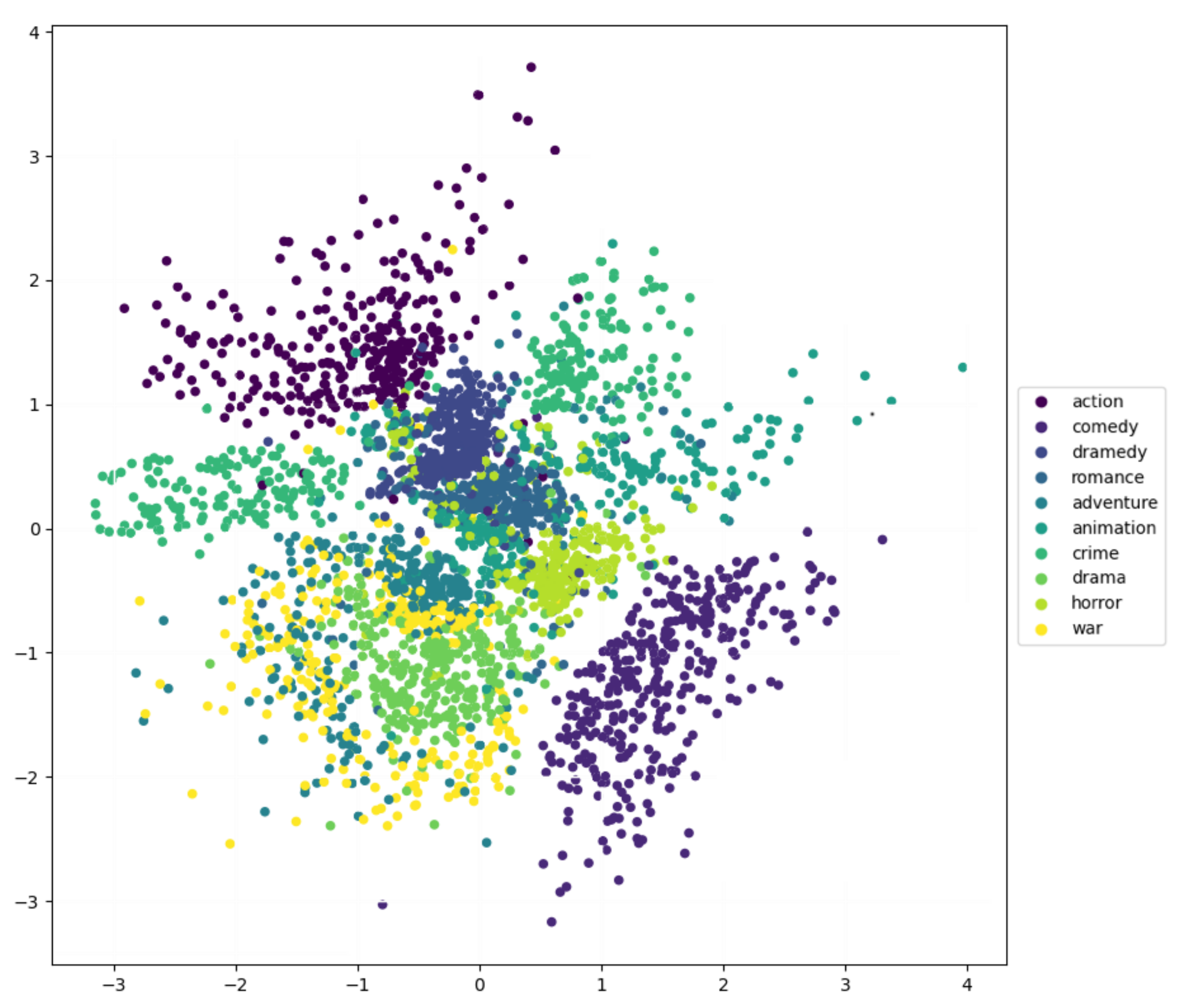
In this part, we explored the internal performance of GVAE-CF more deeply, and we visually learned the latent representations of GVAE-CF on the MoviesLens dataset. We randomly obtained 2000 data with user type tags of user from the MoviesLens-20M dataset (10 types selected). We used principal component analysis (PCA) [36] to reduce the dimensionality of the latent representations and only considered the first three main components.
Since the first principal component was separated from the other types, it was removed. We only observed the differences between the second and third main components in GVAE-CF and the standard VAE. As shown in Figure 2 and Figure 3, GVAE-CF had a stronger ability to capture the relationships between the categories and items, especially in the two movie types of action and comedy. Additionally, GVAE-CF captured the emotional theme of the types, and movies with similar emotions were closer in the feature space. For example, action and adventure both contain emotions, such as passion and madness. However, action and comedy do not have a lot of common emotions, so they are far apart.
4.5. Discussion
In order to verify the accuracy of the GVAE-CF algorithm, this paper compared the existing methods using the MoviesLens and Netflix datasets. The results of the comparison results are shown in Table 1, Table 2 and Table 3.
It can be seen in Table 1 that, in terms of the recommended quality, the GVAE-CF method in this paper was significantly better than the baseline models using the MovileLens-20M dataset, except for RecVAE [16]. Although the recall accuracy of the RecVAE method was slightly higher than that of GVAE-CF, it used noise as input and used noise reduction. The encoder brought more robust embedding learning to be used in combination with the GVAE-CF algorithm. Moreover, the performance of this method on NDCG@100 was better, which shows that our method can determine the relationships between categories and items, because it can push products belonging to the target category to the front of the ranking.
It can be seen in Table 2 and Table 3 that the GVAE-CF method performed better than the other baseline models. For the baseline of WMF matrix factorization recommendation algorithm, recommendation algorithms based on generative models can effectively improve its performance. Compared to previous recommendation algorithms based on the autoencoder model, GVAE-CF was further improved.
5. Conclusions
For the purpose of solving the problem that the distribution of latent variables of VAEs in traditional CF is too simple, this paper presented a novel CF recommendation algorithm that uses a Gaussian mixture model for the distribution of hidden factors for VAE, which relies on a novel optimization function that is essential to the training of our method. In order to verify the performance of the GVAE-CF method, we conducted corresponding experiments on the public datasets of MoviesLens-20M, Netflix, and LASTFM. The experiments proved that the GVAE-CF has high accuracy on the same dataset and can obtain a satisfactory recommendation effect. In addition, we also explored the latent space of GVAE-CF, and we noticed that GVAE-CF has a stronger ability to capture the relationships between categories and items.
In future work, we plan to combine the auxiliary information of users’ behavior logs and the items’ feature information with the network, as well as to continue to improve the accuracy of the network through conditional VAEs. The advantage of GVAE-CF is that it can be combined with many existing models to further improve the performance of the existing VAE model.
Author Contributions
Conceptualization, F.Y.; methodology, F.Y.; software, F.L.; validation, F.L.; formal analysis, F.Y.; investigation, S.L.; resources, S.L.; data curation, S.L. and F.L.; writing, F.L.; visualization, F.L.; supervision, S.L.; project administration, F.L. All authors have read and agreed to the published version of the manuscript.
Funding
This research received no external funding.
Informed Consent Statement
Informed consent was obtained from all subjects involved in the study.
Data Availability Statement
“MoviesLens-20M” at https://grouplens.org/datasets/movielens/20m/; “Netflix” at https://www.kaggle.com/netflix-inc/netflix-prize-data.
Conflicts of Interest
The authors declare no conflict of interest.
Abbreviations
The following abbreviations are used in this manuscript:
| CF | Collaborative filtering |
| GVAE-CF | Variational autoencoder that uses a Gaussian mixture model for the |
| latent factor for CF distribution | |
| VAEs | Variational autoencoders |
| NDCG | Normalized discounted cumulative gain |
| GMM | Gaussian mixture model |
| GAN | Generative adversarial network |
| KL | Kullback-Liebler |
| ELBO | Evidence lower bound |
| RecVAE | Recommender VAE |
| SVD | Singular value decomposition |
References
- Resnick, P.; Varian, H.R. Recommender systems. Commun. ACM 1997, 40, 56–58. [Google Scholar] [CrossRef]
- Pazzani, M.J.; Billsus, D. Content-based recommendation systems. In The Adaptive Web; Springer: Berlin, Germany, 2007; pp. 325–341. [Google Scholar]
- Thomas, X. Content-Based Personalized Recommender System Using Entity Embeddings. arXiv 2020, arXiv:2010.12798. [Google Scholar]
- Zarei, M.R.; Moosavi, M.R. An adaptive similarity measure to tune trust influence in memory-based collaborative filtering. arXiv 2019, arXiv:1912.08934. [Google Scholar]
- Zhao, Z.D.; Shang, M.S. User-based collaborative-filtering recommendation algorithms on hadoop. In Proceedings of the 2010 Third International Conference on Knowledge Discovery and Data Mining, IEEE, Jinggangshan, China, 2–4 April 2010; pp. 478–481. [Google Scholar]
- Zhang, L.; Liu, G.; Wu, J. Beyond Similarity: Relation Embedding with Dual Attentions for Item-based Recommendation. arXiv 2019, arXiv:1911.04099. [Google Scholar]
- Goldberg, D.; Nichols, D.; Oki, B.M.; Terry, D. Using collaborative filtering to weave an information tapestry. Commun. ACM 1992, 35, 61–70. [Google Scholar] [CrossRef]
- Ding, X.; Yu, W.; Xie, Y.; Liu, S. Efficient model-based collaborative filtering with fast adaptive PCA. In Proceedings of the 2020 IEEE 32nd International Conference on Tools with Artificial Intelligence (ICTAI), Baltimore, MD, USA, 9–11 November 2020; pp. 955–960. [Google Scholar]
- Severinski, C.; Salakhutdinov, R. Bayesian Probabilistic Matrix Factorization: A User Frequency Analysis. arXiv 2014, arXiv:1407.7840. [Google Scholar]
- Chae, D.K.; Kang, J.S.; Kim, S.W.; Lee, J.T. Cfgan: A generic collaborative filtering framework based on generative adversarial networks. In Proceedings of the 27th ACM International Conference on Information and Knowledge Management, Torino, Italy, 22–26 October 2018; pp. 137–146. [Google Scholar]
- Kang, W.C.; Fang, C.; Wang, Z.; McAuley, J. Visually-aware fashion recommendation and design with generative image models. In Proceedings of the 2017 IEEE International Conference on Data Mining (ICDM), New Orleans, LA, USA, 18–21 November 2017; pp. 207–216. [Google Scholar]
- Hu, Y.; Koren, Y.; Volinsky, C. Collaborative filtering for implicit feedback datasets. In Proceedings of the 2008 Eighth IEEE International Conference on Data Mining, Pisa, Italy, 15–19 December 2008; pp. 263–272. [Google Scholar]
- Mnih, A.; Salakhutdinov, R.R. Probabilistic matrix factorization. In Advances in Neural Information Processing Systems; MIT Press: London, UK, 2008; pp. 1257–1264. [Google Scholar]
- Liang, D.; Krishnan, R.G.; Hoffman, M.D.; Jebara, T. Variational autoencoders for collaborative filtering. In Proceedings of the 2018 World Wide Web Conference, Lyon, France, 23–27 April 2018; pp. 689–698. [Google Scholar]
- Kim, D.; Suh, B. Enhancing VAEs for collaborative filtering: Flexible priors & gating mechanisms. In Proceedings of the 13th ACM Conference on Recommender Systems, Copenhagen, Denmark, 16–20 September 2019; pp. 403–407. [Google Scholar]
- Shenbin, I.; Alekseev, A.; Tutubalina, E.; Malykh, V.; Nikolenko, S.I. RecVAE: A new variational autoencoder for top-N recommendations with implicit feedback. In Proceedings of the 13th International Conference on Web Search and Data Mining, Houston, TX, USA, 3–7 February 2020; pp. 528–536. [Google Scholar]
- Gopalan, P.; Hofman, J.M.; Blei, D.M. Scalable Recommendation with Hierarchical Poisson Factorization. arXiv 2013, arXiv:1311.1704. [Google Scholar]
- Billsus, D.; Pazzani, M.J. Learning collaborative information filters. In Icml; AAAI: Palo Alto, CA, USA, 1998; Volume 98, pp. 46–54. [Google Scholar]
- Alquier, P.; Cottet, V.; Chopin, N.; Rousseau, J. Bayesian matrix completion: Prior specification. arXiv 2014, arXiv:1406.1440. [Google Scholar]
- Alexandridis, G.; Siolas, G.; Stafylopatis, A. Enhancing social collaborative filtering through the application of non-negative matrix factorization and exponential random graph models. Data Min. Knowl. Discov. 2017, 31, 1031–1059. [Google Scholar] [CrossRef]
- Liang, D.; Altosaar, J.; Charlin, L.; Blei, D.M. Factorization meets the item embedding: Regularizing matrix factorization with item co-occurrence. In Proceedings of the 10th ACM Conference on Recommender Systems; ACM: New York, NY, USA, 2016; pp. 59–66. [Google Scholar]
- Lee, W.; Song, K.; Moon, I.C. Augmented variational autoencoders for collaborative filtering with auxiliary information. In Proceedings of the 2017 ACM on Conference on Information and Knowledge Management; ACM: New York, NY, USA, 2017; pp. 1139–1148. [Google Scholar]
- Askari, B.; Szlichta, J.; Salehi-Abari, A. Joint Variational Autoencoders for Recommendation with Implicit Feedback. arXiv 2020, arXiv:2008.07577. [Google Scholar]
- Altosaar, J. Tutorial-What is a Variational Autoencoder. Available online: https://jaan.io/what-is-variational-autoencoder-vae-tutorial/ (accessed on 30 January 2021).
- Blei, D.M.; Kucukelbir, A.; McAuliffe, J.D. Variational inference: A review for statisticians. J. Am. Stat. Assoc. 2017, 112, 859–877. [Google Scholar] [CrossRef] [Green Version]
- Kingma, D.P.; Welling, M. Auto-encoding variational bayes. arXiv 2013, arXiv:1312.6114. [Google Scholar]
- Rezende, D.J.; Mohamed, S.; Wierstra, D. Stochastic backpropagation and approximate inference in deep generative models. arXiv 2014, arXiv:1401.4082. [Google Scholar]
- Harper, F.M.; Konstan, J.A. The movielens datasets: History and context. ACM Trans. Interact. Intell. Syst. 2015, 5, 1–19. [Google Scholar] [CrossRef]
- Bennett, J.; Lanning, S. The netflix prize. In Proceedings of KDD Cup and Workshop; ACM: New York, NY, USA, 2007; Volume 2007, p. 35. [Google Scholar]
- Dong, X.; Yu, L.; Wu, Z.; Sun, Y.; Yuan, L.; Zhang, F. A hybrid collaborative filtering model with deep structure for recommender systems. In Proceedings of the Thirty-First AAAI Conference on Artificial Intelligence, San Francisco, CA, USA, 4–9 February 2017; pp. 1309–1315. [Google Scholar]
- Li, S.; Kawale, J.; Fu, Y. Deep collaborative filtering via marginalized denoising auto-encoder. In Proceedings of the 24th ACM International on Conference on Information and Knowledge Management; ACM: New York, NY, USA, 2015; pp. 811–820. [Google Scholar]
- Rendle, S.; Freudenthaler, C.; Gantner, Z.; Schmidt-Thieme, L. BPR: Bayesian personalized ranking from implicit feedback. arXiv 2012, arXiv:1205.2618. [Google Scholar]
- Kabbur, S.; Ning, X.; Karypis, G. Fism: Factored item similarity models for top-n recommender systems. In Proceedings of the 19th ACM SIGKDD International Conference on Knowledge Discovery and Data Mining; ACM: New York, NY, USA, 2013; pp. 659–667. [Google Scholar]
- Yang, S.H.; Long, B.; Smola, A.J.; Zha, H.; Zheng, Z. Collaborative competitive filtering: Learning recommender using context of user choice. In Proceedings of the 34th International ACM SIGIR Conference on Research and Development in Information Retrieval, Beijing, China, 24–28 July 2011; pp. 295–304. [Google Scholar]
- Croft, W.B.; Metzler, D.; Strohman, T. Search Engines: Information Retrieval in Practice; Addison-Wesley Reading: Boston, MA, USA, 2010; Volume 520. [Google Scholar]
- Jolliffe, I.T.; Cadima, J. Principal component analysis: A review and recent developments. Philos. Trans. R. Soc. A Math. Phys. Eng. Sci. 2016, 374, 20150202. [Google Scholar] [CrossRef] [PubMed]
- Ning, X.; Karypis, G. Slim: Sparse linear methods for top-n recommender systems. In Proceedings of the 2011 IEEE 11th International Conference on Data Mining, Vancouver, BC, Canada, 11–14 December 2011; pp. 497–506. [Google Scholar]
- Wu, Y.; DuBois, C.; Zheng, A.X.; Ester, M. Collaborative denoising auto-encoders for top-n recommender systems. In Proceedings of the Ninth ACM International Conference on Web Search and Data Mining; ACM: New York, NY, USA, 2016; pp. 153–162. [Google Scholar]
Figure 1.
Variational autoencoder based on a Gaussian mixture model (GMM).

Figure 2.
Second and third components of the principal component analysis (PCA) on variational autoencoder (VAE).
Figure 2.
Second and third components of the principal component analysis (PCA) on variational autoencoder (VAE).

Figure 3.
Second and third components of the PCA on Gaussian mixture model for latent factor distribution for CF (GVAE-CF).
Figure 3.
Second and third components of the PCA on Gaussian mixture model for latent factor distribution for CF (GVAE-CF).


Table 1.
Evaluation scores for GVAE-CF and the baseline models using the MovileLens-20M dataset.
| Method | Recall@20 | Recall@50 | NDCG@100 |
|---|---|---|---|
| WMF [12] | 0.314 | 0.466 | 0.341 |
| SLIM [37] | 0.370 | 0.495 | 0.401 |
| CDAE [38] | 0.391 | 0.523 | 0.418 |
| Mult-DAE [14] | 0.387 | 0.524 | 0.419 |
| Mult-VAE [14] | 0.395 | 0.537 | 0.426 |
| RecVAE [16] | 0.414 | 0.521 | 0.420 |
| GVAE-CF | 0.408 ± 0.002 | 0.520 ± 0.002 | 0.431 ± 0.002 |
Table 2.
Evaluation scores for GVAE-CF and baseline models on Netflix.
| Method | Recall@20 | Recall@50 | NDCG@100 |
|---|---|---|---|
| WMF | 0.314 | 0.466 | 0.341 |
| SLIM | 0.370 | 0.495 | 0.401 |
| CDAE | 0.391 | 0.523 | 0.418 |
| Mult-DAE | 0.387 | 0.524 | 0.419 |
| Mult-VAE | 0.395 | 0.537 | 0.426 |
| RecVAE | 0.414 | 0.521 | 0.420 |
| GVAE-CF | 0.416 ± 0.001 | 0.524 ± 0.001 | 0.431 ± 0.001 |
Table 3.
Evaluation scores for GVAE-CF and baseline models on LASTFM.
| Method | Recall@20 | Recall@50 | NDCG@100 |
|---|---|---|---|
| WMF | 0.252 | 0.346 | 0.259 |
| SLIM | 0.261 | 0.372 | 0.269 |
| CDAE | 0.264 | 0.396 | 0.275 |
| Mult-DAE | 0.277 | 0.401 | 0.351 |
| Mult-VAE | 0.279 | 0.427 | 0.362 |
| RecVAE | 0.296 | 0.421 | 0.372 |
| GVAE-CF | 0.301 ± 0.002 | 0.429 ± 0.002 | 0.381 ± 0.002 |
Publisher’s Note: MDPI stays neutral with regard to jurisdictional claims in published maps and institutional affiliations. |
© 2021 by the authors. Licensee MDPI, Basel, Switzerland. This article is an open access article distributed under the terms and conditions of the Creative Commons Attribution (CC BY) license (http://creativecommons.org/licenses/by/4.0/).
Share and Cite
MDPI and ACS Style
Yang, F.; Liu, F.; Liu, S. Collaborative Filtering Based on a Variational Gaussian Mixture Model. Future Internet 2021, 13, 37. https://0-doi-org.brum.beds.ac.uk/10.3390/fi13020037
AMA Style
Yang F, Liu F, Liu S. Collaborative Filtering Based on a Variational Gaussian Mixture Model. Future Internet. 2021; 13(2):37. https://0-doi-org.brum.beds.ac.uk/10.3390/fi13020037
Chicago/Turabian StyleYang, FengLei, Fei Liu, and ShanShan Liu. 2021. "Collaborative Filtering Based on a Variational Gaussian Mixture Model" Future Internet 13, no. 2: 37. https://0-doi-org.brum.beds.ac.uk/10.3390/fi13020037
Note that from the first issue of 2016, this journal uses article numbers instead of page numbers. See further details here.