How Long Do Return Migrants Stay in Their Home Counties? Trends and Causes

Abstract

Return migration is an important form of rural labor mobility in China, and it has been given growing concern recently by governments in the background of rural revitalization. However, research covering the duration of stay in migrants’ home counties, a basic question of labor mobility and a precondition for policy making, is far from enough. The aim of this paper is to analyze the period of return for these migrants based on employment history data by tracking their mobility among rural laborers from 1998 to 2015. The data was collected from a randomized, nationally representative sample of 100 rural villages in five provinces of China. We find that only 22.3 percent of migrants returned from 1998 to 2015, and most return migrants still remained in their home counties as of 2015. Using the OLS, Tobit, and Heckman sample selection models, the results show that return migrants who are old, more educated, unmarried, and with children are more likely to stay longer in their home counties. From a development perspective, return migrants are expected to play an important role in the process of rural revitalization.

1. Introduction

The migration of rural laborers in China plays an important role in promoting the growth of the whole economy. On the one hand, rural laborers flow into cities to supply cheap labor resources and stimulate urbanization [1,2]. On the other hand, many studies have shown that the migration of rural laborers was historically met with increased rural incomes [3,4,5,6]. Remittances not only increase the accumulation of assets for farmers and promote self-employment, but they also increase consumption among those farmers and have a short-term effect on poverty alleviation [2,7,8,9,10,11,12,13,14]. An additional migrant laborer in the household improves the per capita income of that household by 8.5 to 13.1 percent [11]. Labor migration was shown to reduce grain output by 2 percentage points, but increase net income by 16 percentage points [14].

However, the hukou registration system hinders most rural laborers that are permanent residents of a city. The hukou, a household registration system, documents information of the family members. There are rural hukou and urban hukou in China. Residents with different types of hukou have different types of access to social welfare, such as pensions, medical security, and educational opportunities. There exists labor market discrimination against rural hukou holders in cities [1,15,16,17,18,19,20]. More importantly, migrants with rural hukou working in big cities have little to no access to welfare programs that are provided by local city governments, such as education, healthcare, and pensions [19,21]. Even if cities attempt to extend urban welfare provisions to migrants, their participation in such programs remains relatively low due to hukou [22,23]. The current healthcare programs have not been effective in alleviating the financial burden of healthcare and promoting formal medical utilization among migrant workers [24]. This is possibly due to the lack of a systematic financing scheme for outpatient treatment and the segmentation among the platforms of insurance. Therefore, return migration is an integral part of rural-to-urban labor migration in China. Most studies reveal that the modernization of industry and transfer of labor-intensive industries from coastal to inland areas and other Asian countries were the major pulling and driving factors for return migration after 2008 [25,26,27]. The demand for low-skilled labor has been reduced in coastal areas because of this change. Additionally, with the development of the inland economy, rural migrants have been able to find jobs in local areas. Though wages were lower, they could afford the lower cost of living and stay together with family members [14,28].

However, return migration affects the place of residence and place of origin. Some coastal cities suffer from labor shortages due to return migration, which has resulted in the rapid rise of labor costs [29]. Regarding the place of origin, return migrants on the one hand increase the local employment pressure, and on the other hand, they can promote local economic development by investing in assets and conducting entrepreneurship with their capital and technology that they have accumulated in the cities [14,15,30,31].

Given this information, the Chinese government has been paying close attention to the latest round of return migration due to its large scale and lower employment rate. The “No. 1 Document” of the central government in 2017 highlights the importance of supporting employment and entrepreneurship among return migrants [32]. The five ministries of the State Council jointly enacted an entrepreneurship training plan for return migrants (the fanxiang chuangye peixun jihua) from 2016 to 2020 [33]. The local governments also carried out a series of policies to encourage entrepreneurship among return migrants [34,35]. That return migrants have become the major force behind revitalization of the countryside was put forth in the 19th National Congress of Communist Party of China [32].

Scholars examining recent labor trends in China have typically focused on return migration in two periods. Some of them analyze the status, causes, and economic behavior of return migration around the year 2000. The rest examine changes surrounding the financial crisis in 2008, and especially during years that followed.

Most previous studies described individual characteristics of return migrants and analyzed their impact on return migration [14,25,27,36,37,38]. They found that individual characteristics (gender, age, and education) and household characteristics (household size and structure) were correlated with whether migrants returned or not. For example, one study found that return migrants were more likely to be elder, married, and have their spouses at home [14].

Although scholars have conducted plenty of studies on return migration, two important problems remain. The first concerns how many migrants have returned in recent years and its time trend of return migration. Most previous studies have not answered this question because they only used the cross-sectional data from villages after the migrants returned, which lacked the corresponding information for contemporaneous migrants. If information on migration and return migration were used together, we could describe the percentage of return migration more accurately. Only one paper studied this question for the period before 1999, but it did not account for potential sample selection bias and the results did not reflect the situation at the time due to the use of older data [14]. Secondly, and most importantly, a vast majority of research has not yet focused on the period of return and its determinants. Others found that return migrants felt more likely to migrate than those who had never migrated [39]. However, due to a lack of data, they neither studied how many years the return migrants stayed in their home counties until their next migration, nor which factors influenced this period.

The two-step model is a general framework for analyzing migration within most contexts. Some sociologists have used this model to research return intentions [40,41,42,43,44]. They evaluated migration as a potential course of action and the realization of actual mobility or immobility at a given moment. This approach is united by their attention to thoughts and feelings that precede migration outcomes. Plenty of economists also use two-step model from the aspect of labor market behaviors, such as wage, bonus, promotion, training, and migration, to mitigate sample selection bias [45,46,47]. For example, laborers will not enter the workforce if their reservation wage is higher than the wage offered. People do not only make a choice between off-farm labor and leisure; they can also choose to raise livestock or farm. Their individual reservation wage is therefore determined by other opportunities and tradeoffs between job and leisure. If that reservation wage is higher than the wage that is offered for an individual’s skill set, that person would not enter the job market. However, from the perspective of research, we only observe wages for individuals who are offered a wage higher than their reservation wage. If we do not correct for this selectivity bias, the estimators will be biased. As for our study, we may only observe the mobility behaviors of laborers who already have an off-farm job, which results in selection bias.

As such, the aim of this study is to analyze the period of return to one’s home county and its influencing factors among return migrants in recent years to answer the basic question for rural labor mobility while also being a precondition for policy, such as for providing employment services, healthcare, and pensions for return migrants. With this goal in mind, we want to answer following three questions. First, what are the scale and trend of return migration in recent years? Second, how long do return migrants stay in their home counties? Third, which factors affect this period?

This paper is organized as follows. The next section introduces the materials and methods that we used in this study. We show our results in Section 3. Section 4 contains conclusions and discussions.

2. Materials and Methods

2.1. Data

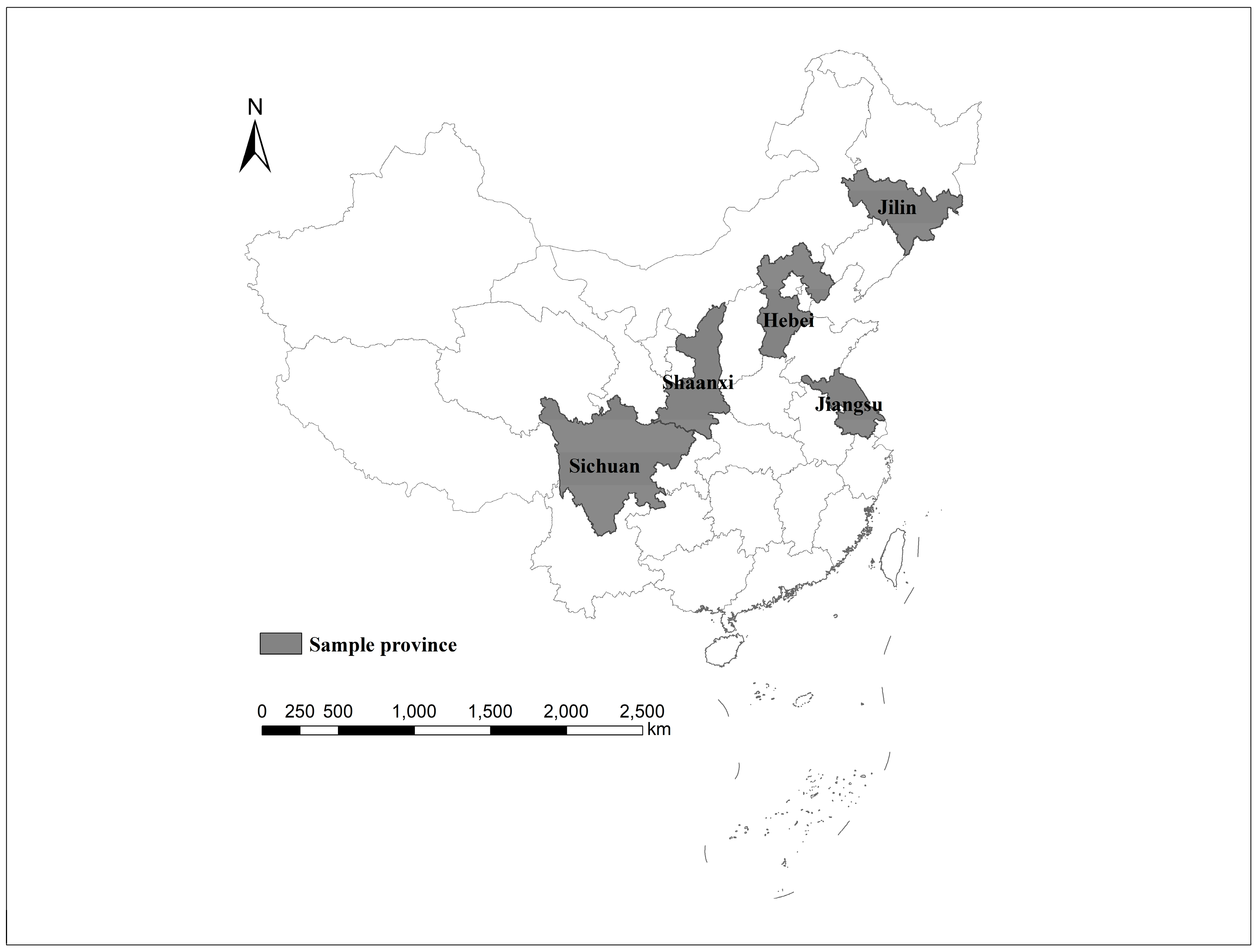
This paper draws from panel data, named China Rural Development Survey (CRDS), collected by the Center for Chinese Agricultural Policy of the Chinese Academy of Sciences. A multi-round survey was administered to households and village leaders of 100 villages in 25 counties across five provinces in 2005, 2008, 2012, and 2016. In the first round of the survey in 2005, each sample province was randomly selected from China’s major agro-ecological zones. Five sample counties were then selected from each province in a two-step procedure. First, the enumeration team listed all the counties in each province in descending order of per capita gross value of industrial output (GVIO), which is a good predictor of standard of living and development potential, and often more reliable than net per capita income [48]. Five counties per province were then randomly selected from the resulting list (Figure 1).

From each selected county, the team chose sample townships and villages. Two townships were chosen from each county, one from each of two groups per county: a “more well-off” group and a “poorer” group. Following the same procedure, two villages per township were chosen. Finally, the survey teams randomly chose 20 households from each village. Our sampling strategy yields a sample that is not strictly nationally representative, because it does not, for example, use census-based population counts in each survey year as sampling weights, but is nevertheless broadly reflective of China’s rapidly changing rural population. Appendix

Table A1. Descriptive statistical averages of rural China, 2015.

Sample Characteristics	CRDS	NBS
Age (years)	36.1	36.7
Schooling (years)	9.0	8.6
Sex ratio (males per 100 females)	117.9	105.0
Household size (persons)	4.6	3.3
Non-Han (%)	4.6	8.6
Farmland (mu)	7.0	5.7

Data Source: China Rural Development Survey (CRDS).

shows comparisons between our sample and data from China’s National Bureau of Statistics (NBS), suggesting that they are reasonably similar. They also conducted three rounds of follow-up surveys in 2008, 2012, and 2016.

The survey team gathered detailed information on demographic, family, and village characteristics in each wave of the survey. Individual demographic characteristics included gender, birth year, educational attainment, marriage year, and employment status. Specifically, in the block of employment, they also documented the employment history of three generations in the family in each year from 1998 to 2015, including whether they were engaged in off-farm labor, whether they participated in self-employment, their occupation, and location of their job in terms of county. Using this data helps us to construct the status of return migration and its evolution.

According to the individual characteristics, we also are able to obtain information concerning household structure. Despite this, due to the definition of the three generations in the survey, we did not collect information on children of individuals who were brothers or sisters of the household head. At the village level, we also obtained the migration status of laborers.

2.2. Construction of Variables

In order to answer the questions that are put forward in the first section, we separate the following indicators into three groups and give detailed definitions.

Group 1: Indicators for constructed variables

Rural labor includes all men and women between 16 and 64 years old who had rural hukou, and who were not retired or disabled in each year from 1998 to 2015. Students were also excluded from our sample.

Off-farm employment is defined as held by those who were occupied in off-farm work or self-employment for at least six months of the year from 1998 to 2015.

Migrants are referred as to those who were employed off-farm and worked outside of the county for more than six months in each year from 1998 to 2015. There were 5882 migrants between 1998 and 2015, including both continuous and temporary migrants.

Return migrants refers to those who had been migrants previously and returned to the county for more than six months in one year from 1998 to 2015. For example, an individual who was a migrant in 1998, 1999, 2000, and 2001, but then he returned to his home county and stayed there for more than six months in 2002. We would call them a return migrant in 2002.

Group 2: Dependent variable

Period of return means the number of years a return migrant remained in their home county following their return. For example, if a migrant returned the county in 2002, and migrated again in 2003, their period of return would be 0 years; if they returned to the county in 2002, and migrated again in 2004, their period of return would be one year, and so on.

Group 3: Independent variables

Age cohort: we collected the birth year of each family member. This allows us to calculate their age in each year from 1998 to 2015. We classify their ages into four cohorts: 16–25; 26–35; 36–45; and, over 45.

Occupation: we collected detailed information about occupation, including position and industry. For example, were they a worker in a shoe factory, service staff in a restaurant, a teacher in primary school, and so on. Though there were numerous types, we classified them in three groups: manual laborers, service staff, and others.

Other independent variables: educational attainment, marital status, whether returning from another province, whether having children (separated into four different age cohorts), and migrants in total village labor force. Educational attainment is measured by the years of formal schooling. Marital status is obtained using the marriage year in each year between 1998 and 2015. Using the birth year of each child, we also gain whether the return migrants had children in each age cohort.

Table 1. Description of variables.

	Variables	Definition/Measurement	Obs.	Mean	Std. D.	Min	Max
(1)	Male	1 = yes; 0 = no	1190	0.53	0.50	0	1
(2)	Aged 16–25	Aged 16–25 before the year of return (1 = yes; 0 = no)	1190	0.52	0.50	0	1
(3)	Aged 26–35	Aged 26–35 before the year of return (1 = yes; 0 = no)	1190	0.23	0.42	0	1
(4)	Aged 36–45	Aged 36–45 before the year of return (1 = yes; 0 = no)	1190	0.14	0.35	0	1
(5)	Aged over 45	Aged above 45 before the year of return (1 = yes; 0 = no)	1190	0.11	0.31	0	1
(6)	Educational attainment	Years	1190	8.57	2.98	0	16
(7)	Married	Have married before the year of return (1 = yes; 0 = no)	1190	0.56	0.50	0	1
(8)	Return from another province	1 = yes; 0 = no	1190	0.65	0.48	0	1
(9)	Manual laborers	Manual laborers before the year of return (1 = yes; 0 = no)	1190	0.56	0.50	0	1
(10)	Service staff	Service staff before the year of return (1 = yes; 0 = no)	1190	0.30	0.46	0	1
(11)	Other occupation	Other occupation before the year of return (1 = yes; 0 = no)	1190	0.14	0.34	0	1
(12)	Children 0–3	Having child aged 0–3 years old before the year of return (1 = yes; 0 = no)	1112	0.11	0.31	0	1
(13)	Children 4–5	Having child aged 4–5 years old before the year of return (1 = yes; 0 = no)	1112	0.06	0.23	0	1
(14)	Children 6–12	Having child aged 6–12 years old before the year of return (1 = yes; 0 = no)	1112	0.15	0.35	0	1
(15)	Children 13–15	Having child aged 13–15 years old before the year of return (1 = yes; 0 = no)	1112	0.05	0.21	0	1
(16)	Migrants in village labor force	Percent of migrants in total village labor in 1997	1190	11.59	11.35	0	46.93

Data Source: China Rural Development Survey (CRDS).

shows the description of independent variables. The description of individual and household characteristics among the five provinces is listed in Appendix

Table A2. Description of individual characteristic and household characteristic among five provinces.

	Jiangsu	Sichuan	Shaanxi	Jilin	Hebei
Male	0.57	0.51	0.51	0.52	0.57
Aged 16–25	0.24	0.41	0.68	0.57	0.61
Aged 26–35	0.20	0.28	0.19	0.23	0.21
Aged 36–45	0.13	0.23	0.09	0.11	0.08
Aged over 45	0.44	0.07	0.04	0.09	0.11
Educational attainment	7.87	8.52	8.54	9.06	8.73
Married	0.83	0.67	0.44	0.40	0.51
Return from another province	0.20	0.84	0.52	0.64	0.64
Manual laborers	0.60	0.72	0.51	0.26	0.52
Service staff	0.22	0.15	0.37	0.57	0.36
Other occupation	0.19	0.13	0.12	0.17	0.12
Children 0–3	0.07	0.12	0.12	0.06	0.11
Children 4–5	0.04	0.07	0.04	0.03	0.06
Children 6–12	0.18	0.20	0.13	0.08	0.11
Children 13–15	0.02	0.08	0.03	0.05	0.02
Migrants in village labor force	13.92	17.65	7.04	8.62	6.98

Data Source: China Rural Development Survey (CRDS).

.

2.3. Empirical Approach

In order to achieve the aim of this study, which is to make up for a gap in the field of returning labor mobility by studying the length of stay in return migrants’ home counties following their return, we need to clarify the impact of various factors on the period of return. However, there is a certain correlation between these factors. Although multi-state life tables can show the period of return for people with different characteristics (including age, sex, marital status, etc.), it is not easy to operate this method when considering multiple characteristics at the same time. On the other hand, the econometric regression model can be convenient for estimating the impact of multiple factors on the dependent variables at the same time, and it can report the magnitude and direction of the impact of these factors. Therefore, we conduct a regression approach to analyze the data.

We conduct three types of analysis: Ordinary Least Squares (OLS), Tobit regression, and the Heckman sample selection model to explore the relationship between the period of return and the characteristics of return migrants.

2.3.1. OLS Regression

Our first type of analysis uses OLS regression as the benchmark model due to our dependent variable being period of return, a continuous variable. We conducted OLS analysis to examine the basic relationship between the characteristics of return migrants and their period of return while controlling for the observable covariates that may confound that relationship. The basic specification for the OLS analysis is

$$Y_i=\mathsf{\alpha }+\beta X_i+\gamma D_i+\delta T_i+u_i$$

(1)

where $Y_i$ represents the outcome variable of interest: the period of return. $\alpha$ describes a baseline period of return, other factors notwithstanding. Considering that there are differences in individual, family, and village characteristics among samples in different provinces, we add provincial dummy variables into the regression models to control for these differences. $D_i$ is a group of province dummy variables. $T_i$ represents the dummy variable of the year that migrants return. $u_i$ is the error term. $X_i$ represents the vector of observable covariates. It includes the individual, household, and village characteristics that are shown in Table 1. In the absence of omitted variable bias, $\beta$, $\gamma$, and $\delta$ will be the vector of coefficients for the independent variables.

2.3.2. Robustness Check

The robustness check is a commonly method used to study labor mobility, which aims to test whether the regression results are consistent. If different regression methods are used to draw a consistent conclusion, these results are considered credible.

There are two main econometric issues in using OLS estimation. The first is the fact that the period of return is truncated between 0 and 16. As this may cause biases if usual linear regression models are used, a Tobit method is adopted to be a robustness check. The second issue is the possible selectivity bias due to only observing the period of return of those who have already returned, which also may result in biases if we do not correct for this selectivity bias [49]. The return migrants may be different from those who remain in the cities. We only observe the “period of return” of those who have returned, which may result in sample selection bias when we use the OLS model. In order to control for this potential selection bias, we use the Heckman Sample Selection model.

While using the Heckman sample selection model, we first estimate a Probit for all rural laborers who were migrants at any point between 1998 and 2015, where the dependent variable is one if the migrants returned and zero otherwise. Using the results from the Probit estimation, we compute an inverse Mills ratio that corrects for the possible truncation of the dependent variable in estimation of Equation (1). In the Probit equation, we include the marketization index of each province where the migrants worked before returning.

The marketization index of China has been calculated by the economists [50,51] year-by-year since 1997. In their index report, we can find the marketization index of all the provinces in the mainland over the years from 1997 to 2014. The index of 2015 is absent due to a lack of data. We use the average index from 2012 to 2014 to replace the marketization index of 2015. The index was obtained from five aspects: the relationship between the government and the market, the development of the private economy, the development of factor and product markets, and the development of intermediary agencies and the legal environment. The higher the marketization index, the stronger the province’s inclusiveness, and the easier it is for migrants to integrate into cities. We believe that this variable can identify the return effect, since it should not affect the period of return, but it may affect a migrant’s decision about whether or not to return.

3. Results

3.1. Return Migrants and Their Period of Return from 1999 to 2015

Of our 5882 migrants, 22.3 percent returned between 1999 and 2015. In the previous study, 38.4 percent of all workers with migration experience were returnees before 1999, which was much higher than the results that we find [14]. We think that it can be explained mainly by the continuous reform of the hukou system since the middle of 1990s. 1997 saw the first time that the Chinese government allowed rural people who were satisfied with certain conditions, such as employment and residence in cities, to obtain urban hukou [52]. In 1998, the household registration system became more beneficial to rural people [53]. The planned target management was no longer applicable to those who applied for permanent residence in small cities and towns following 2001 [54]. In 2012, rural people began to have opportunity to settle down in medium-sized cities [55].

The percentage of return migrants varies among the five sample provinces (Figure 2). In the Jiangsu province, one of the most developed areas in China, the rate of return was smaller than 7 percent between 1999 and 2015. In the Sichuan province, one of the provinces with the most labor emigration, the financial crisis had a significant impact on labor return compared to other provinces. The rate of return was around 32.6 percent from 1999 to 2015. The rate of return in Shaanxi, another western province, was two percentage points lower than that of Sichuan. The rate of return migrants in Jilin was about 26.7 percent, which is the smallest in all four developing provinces. Lastly, the rate of return in Hebei was similar to that of Jilin.

There may be three factors behind the huge regional disparity in percentage of return migrants. First of all, the flow of migrants originates mainly from the developing provinces and it goes into the developed eastern provinces [56,57]. The percentage of migration is much lower in developed provinces than in developing provinces [58,59]. Secondly, migrants from developing provinces are more likely to search for jobs in other provinces, and thus face more risk if the provinces that they work in suffer an economic crisis. Finally, according to NBS data, inland provinces have been experiencing rapid economic growth since 2008, especially in secondary and tertiary industries (Appendix A

Table A4. Impact of individual, household, village characteristics on the period of return, Tobit.

	VARIABLES	Dependent Variable: Period of Return (Years)
		(1)	(2)	(3)
	Individual characteristics
(1)	Male	−0.178	−0.187	−0.195
		(−0.898)	(−0.906)	(−0.948)
(2)	Aged 26–35	0.616 **	0.067	0.082
		(2.293)	(0.210)	(0.260)
(3)	Aged 36–45	1.494 ***	0.918 **	0.924 **
		(4.550)	(2.383)	(2.408)
(4)	Aged over 45	1.537 ***	1.776 ***	1.834 ***
		(3.976)	(4.144)	(4.291)
(5)	Educational attainment	0.052	0.057	0.057
		(1.540)	(1.632)	(1.635)
(6)	Married	−0.669 ***	−1.107 ***	−1.125 ***
		(−2.866)	(−4.202)	(−4.286)
(7)	Return from another province	−0.217	−0.195	−0.190
		(−1.001)	(−0.867)	(−0.848)
(8)	Manual laborers	−0.096	−0.018	−0.035
		(−0.424)	(−0.077)	(−0.152)
(9)	Service staff	0.124	0.399	0.403
		(0.314)	(0.984)	(1.000)
	Household characteristics
(10)	Children 0–3		0.538	0.582
			(1.506)	(1.633)
(11)	Children 4–5		1.006 **	1.036 **
			(2.160)	(2.232)
(12)	Children 6–12		1.004 ***	1.017 ***
			(2.947)	(2.997)
(13)	Children 13–15		1.906 ***	1.918 ***
			(3.683)	(3.721)
	Village characteristics
(14)	Migrants in village labor force			−0.029 ***
				(−3.055)
(15)	Province dummy	YES	YES	YES
(16)	Return year dummy	YES	YES	YES
(17)	Constant	12.389 ***	12.461 ***	12.966 ***
		(15.745)	(15.496)	(15.836)
(18)	Observations	1190	1112	1112

Note: (a) marginal effect is reported; (b) t statistics in parentheses; (c) *** p < 0.01, ** p < 0.05, * p < 0.1. Data Source: China Rural Development Survey (CRDS).

), which has created more job opportunities than before [60].

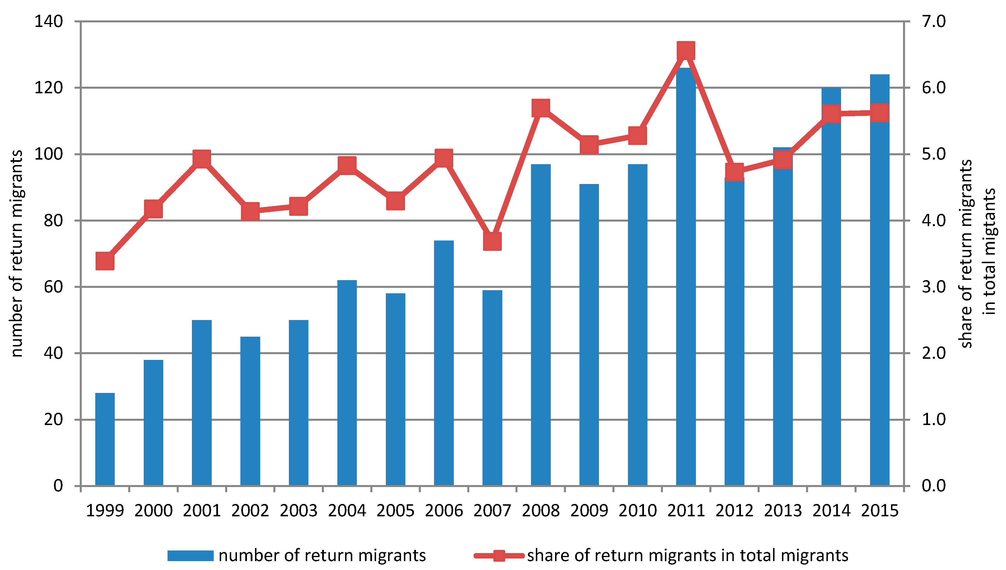
Figure 3 presents the trends of increasing return migration in rural China. In our sample, the number of return migrants was only 28 in 1999, and accounted for only 3.4 percent of the 826 migrants in that year. In 2015, the number of return migrants increased to 124, which amounted to 5.6 percent of all migrants. The fact that there are far more returnees in recent years than in earlier years may be due to the increasing migration and that more migration yields more returnees [14]. Our data shows that 20.6% or 826 rural off-farm labors migrated in 1999, and nearly half of rural off-farm laborers migrated in 2015. As for first-time migrants, the number has also increased significantly since 1999. However, it is important to note that the number of return migrants and the percentage among all migrants were not always increasing during this period.

There were three big dips in return migrants from 1999 to 2015. In the beginning, the number of return migrants continuously increased, reaching 50, about 4.6% of migrants, in 2001. This was met with a 10 percent dip to 45 in 2002. Following this drop, the number of return migrants continued to increase until 2006, with 74 return migrants that accounted for 4.0% of all migrants. In 2007, another decline in the number of return migrants occurred, this time by about 20 percent.

In view of the financial crisis, the number of return migrants increased dramatically to 97 in 2008, or about 4.5% of all migrants. This trend was interrupted temporarily by the financial crisis in late 2008, which caused about 20 million rural-urban migrant workers to lose their urban jobs at the beginning of 2009 [61,62]. Return migrants increased from 2008 to 2011 by nearly 30%. There was the third drop in 2012, and the number of return migrants decreased by 26 percent from its level in 2011.

These three drops closely mirror the trajectory of the economy at large. In previous studies, they found that the economic cycle was about six years during over the period of 1980 to 2000 [37]. In our study, the cycle for return migrants is about five years.

There were 1314 returning migrants in total during 1999 to 2015. However, of those who returned in 2015, we do not know whether they emigrated again. Of the 1190 return migrants, most of them stayed in their home counties for a considerable amount of time (

Table 2. Distribution of period of return by return year (% of return migrants).

		0 Year (1)	1 Year (2)	2 Years (3)	3 Years (4)	4 Years (5)	5 Years (6)	6 Years (7)	7 Years (8)	8 Years (9)	9 Years (10)	10 Years (11)	11 Years (12)	12 Years (13)	13 Years (14)	14 Years (15)	15 Years (16)	16 Years (17)
(1)	1999	3.6	14.3	3.6	3.6	0	0	0	3.6	0	0	3.6	0	3.6	3.6	0.0	3.6	(57.1 *)
(2)	2000	0	7.9	5.3	2.6	2.6	0	0	2.6	0	0	0	0	5.3	2.6	0.0	(71.1 *)
(3)	2001	10	10	2	6	0	0	4	4	2	4	0	0	2	2	(54 *)
(4)	2002	11.1	2.2	4.4	0	4.4	2.2	4.4	2.2	2.2	2.2	6.7	2.2	0	(55.6 *)
(5)	2003	4	12	6	4	8	0	2	0	0	4	4	0	(56 *)
(6)	2004	8.1	19.4	1.6	3.2	1.6	4.8	1.6	0	0	3.2	3.2	(53.2 *)
(7)	2005	12.1	6.9	8.6	5.2	3.4	1.7	1.7	1.7	6.9	6.9	(44.8 *)
(8)	2006	5.4	16.2	4.1	1.4	4.1	1.4	8.1	1.4	6.8	(51.4 *)
(9)	2007	13.6	10.2	1.7	1.7	3.4	0	1.7	3.4	(64.4 *)
(10)	2008	5.2	5.2	3.1	4.1	7.2	1.0	4.1	(70.1 *)
(11)	2009	5.5	8.8	1.1	5.5	3.3	4.4	(71.4 *)
(12)	2010	8.3	6.2	7.2	5.2	5.2	(68.0 *)
(13)	2011	4	10.3	5.6	6.4	(73.8 *)
(14)	2012	7.5	7.5	4.3	(80.7 *)
(15)	2013	7.8	5.9	(86.3 *)
(16)	2014	14.2	(85.8 *)

Note: * indicates total return migrants who remained in their home county. Data Source: China Rural Development Survey (CRDS).

). For example, for those who returned in 1999, 57.1 percent of them were still within the county in 2015. Among those who returned in 2000, 71.1 percent of were still within the county in 2015. For those who returned in 2008 and 2009, 70.1 percent and 71.4 percent of them stayed in their home counties by 2015, respectively.

On the whole, return migrants were more likely to remain in their home counties following 2008. The percentage of return migrants who emigrated again within one year were 27.5, 19, 21.6, and 23.8 in the return years of 2004, 2005, 2006, and 2007, respectively (sum of columns 1 and 2). However, the percentage of return migrants who emigrated again within 1 year declined to 10.4 in 2008, and around 14 percent from 2009 to 2013. If we consider those migrants whose period of return was five years, rather than one, the result was similar.

It is not surprising that most of the returnees returned from coastal provinces, which were the most seriously affected areas by the economic crisis of 2008. On the one hand, these provinces made great effort to transfer and upgrade their industries, which required a higher quality labor force [63,64,65,66]. The low-educated and unskilled labor force is excluded from this market. On the other hand, the cost of living in coastal provinces has been rising [67], and the wage premium in these areas has disappeared [68]. Some migrant workers with lower incomes were prevented from migrating to these areas.

3.2. Econometric Analysis of Determinants of Period of Return

3.2.1. OLS Estimation

To understand the factors determining the period of return, we firstly use the sample of return migrants to conduct the OLS estimation and run three regressions. In the first set of regressions, we only include the individual characteristics, province dummies, and the year of return dummies. In the second regression, we add household characteristics. Then we add migrant status in the village in the third regression. The results are presented in

Table 3. Impact of individual, household, village characteristic on the period of return, Ordinary Least Squares (OLS).

Variables	Dependent Variable: Period of Return (Years)
	(1)	(2)	(3)
Individual characteristic
Male	−0.135	−0.134	−0.141
	(−0.731)	(−0.699)	(−0.737)
Aged 26–35	0.567 **	0.096	0.108
	(2.274)	(0.327)	(0.367)
Aged 36–45	1.300 ***	0.809 **	0.810 **
	(4.266)	(2.256)	(2.267)
Aged over 45	1.289 ***	1.482 ***	1.528 ***
	(3.583)	(3.700)	(3.823)
Educational attainment	0.041	0.048	0.048
	(1.299)	(1.465)	(1.466)
Married	−0.610 ***	−0.998 ***	−1.013 ***
	(−2.815)	(−4.068)	(−4.143)
Return from another province	−0.189	−0.164	−0.158
	(−0.937)	(−0.783)	(−0.757)
Manual laborers	−0.091	−0.017	−0.034
	(−0.435)	(−0.079)	(−0.154)
Service staff	0.086	0.322	0.323
	(0.234)	(0.849)	(0.856)
Household characteristic
Children 0–3		0.517	0.557 *
		(1.558)	(1.681)
Children 4–5		0.822 *	0.847 *
		(1.891)	(1.956)
Children 6–12		0.834 ***	0.841 ***
		(2.636)	(2.666)
Children 13–15		1.707 ***	1.719 ***
		(3.527)	(3.562)
Village characteristic
Migrants in village labor force			−0.025 ***
			(−2.806)
Province dummy	YES	YES	YES
Return year dummy	YES	YES	YES
Constant	11.510 ***	11.529 ***	11.959 ***
	(16.250)	(15.849)	(16.136)
Observations	1190	1112	1112
R-squared	0.518	0.522	0.525

Note: (a) t statistics in parentheses; (b) *** p < 0.01, ** p < 0.05, * p < 0.1; (c) the observations in the second and third regressions are both 1112, because we didn’t collect the children’s information of the brothers and sisters of the household head in the survey. Data Source: China Rural Development Survey (CRDS).

. The following discussion of these results is based on the third regression.

According to the results of the OLS estimation, a male return migrant had a shorter period of return than a female by 0.141 years, or about two months, but this effect was not significant (Table 3, row 1, column 3).

Older return migrants are more likely to stay longer in their home counties after return. The period of return for those aged between 26 and 35 years was not significantly different from that of those aged between 16 and 25 years (Table 3, row 2, column 3). On the other hand, a return migrant aged between 36 and 45 was likely to stay in their home county for 0.81 years longer than one aged between 16 and 25, and this effect is significant at the five percent level (Table 3, row 3, column 3). For return migrants over the age of 45, their period of return was 1.528 years longer than for those aged between 16 and 25, and this effect was significant at the one percent level (Table 3, row 4, column 3). As for return migrants over 35 years old, they often had both children and elderly family members. This probably means they faced heavier social and familial constraints. Additionally, most rural off-farm laborers were engaged in manual work, and the elders preferred to stay in local areas and were more unlikely to go out because they had no advantage in occupying in industries requiring manual labor.

Although return migrants with high educational attainment are more likely to stay longer within their home counties, the effect is not significant (Table 3, row 5, column 3). Married return migrants were more likely to have a 1.013 years shorter period of return than unmarried return migrants (p < 0.01, Table 3, row 6, column 3). In our sample, the average age of unmarried migrants before their return was 22.9 years old, which is just about the age of marriage in the Chinese countryside. It is possible that unmarried return migrants may have spent more time in their home preparing for marriage. While migrants returning from another province were likely to stay in their hometown for a shorter period, the effect was not significant, even at the 10 percent level (Table 3, row 7, column 3). The occupation of those who had been employed before returning did not significantly affect the period of return (Table 3, rows 8 and 9, column 3).

Having children had a significant effect on the period of return. Specifically, a return migrant with children aged between 0 and three years old was likely to stay in their home county for 0.557 years longer than one who did not have children from this cohort (p < 0.1, Table 3, row 10, column 3). A return migrant with children aged between four and five years old was likely to stay in their home county for 0.847 years longer than one who did not have children from this cohort (p < 0.1, Table 3, row 11, column 3). If a return migrant had children between six and 12 years old, corresponding to primary school, they would stay in their home county for 0.841 years longer than one without children in this cohort (p < 0.01, Table 3, row 12, column 3). A return migrant with children between 13 and 15 years old, corresponding to junior high school, would stay in their home county for 1.719 years longer than one who did not have children in this cohort (p < 0.01, Table 3, row 13, column 3).

The percentage of migrants in village labor force had significantly negative effect on the period of return. If the percentage of migrants in village labor force increased by one percent, the period of return of return migrants would decrease by 0.025 years (p < 0.01, Table 3, row 14, column 3). The percentage of migrants in the village labor force reflects the circumstances of employment that are encountered by return migrants. It is usually high if the off-farm employment opportunities in local areas are limited and rural laborers must migrate for a living.

3.2.2. Robustness Check

We conduct the Tobit and Heckman sample selection model to do robustness checks. The results of the Tobit regression tell a similar story to those of the OLS estimation. For brevity, we only report the results of the Heckman sample selection model. The results of Tobit analysis are shown in Appendix A Table A2.

The Heckman sample selection model demonstrates results that are similar to and consistent with those of the OLS regression. However, the magnitudes of the coefficients are different from those in the OLS regressions, and they have much higher significance (

Table 4. Impact of individual, household, village characteristic on the period of return, Heckman sample selection model.

Variables	Selection Equation (1)	Period of Return (2)	Selection Equation (3)	Period of Return (4)	Selection Equation (5)	Period of Return (6)
Individual characteristic
Male	−0.114 ***	−0.103	0.189 ***	−0.175	0.187 ***	−0.181
	(−2.656)	(−0.555)	(3.404)	(−0.907)	(3.372)	(−0.939)
Aged 26–35	−0.795 ***	0.945 **	−1.071 ***	0.338	−1.071 ***	0.342
	(−13.364)	(2.406)	(−12.102)	(0.906)	(−12.094)	(0.923)
Aged 36–45	−1.097 ***	1.802 ***	−1.933 ***	1.325 **	−1.929 ***	1.310 **
	(−16.408)	(3.537)	(−20.399)	(2.151)	(−20.332)	(2.143)
Aged over 45	−0.951 ***	1.743 ***	−2.054 ***	2.071 ***	−2.049 ***	2.099 ***
	(−12.778)	(3.410)	(−19.734)	(2.997)	(−19.653)	(3.058)
Educational attainment	−0.077 ***	0.078 *	−0.069 ***	0.066 *	−0.069 ***	0.065 *
	(−11.115)	(1.768)	(−7.972)	(1.771)	(−8.009)	(1.762)
Married	−0.269 ***	−0.512 **	−0.797 ***	−0.878 ***	−0.800 ***	−0.897 ***
	(−4.880)	(−2.185)	(−9.735)	(−3.143)	(−9.755)	(−3.223)
Return from another province	0.616 ***	−0.358	0.555 ***	−0.236	0.558 ***	−0.228
	(14.374)	(−1.481)	(10.506)	(−1.085)	(10.538)	(−1.055)
Manual laborers	−0.088 *	−0.083	−0.171 ***	0.000	−0.176 ***	−0.015
	(−1.828)	(−0.398)	(−2.789)	(0.001)	(−2.850)	(−0.072)
Service staff	−0.140	0.049	−0.044	0.283	−0.044	0.286
	(−1.567)	(0.135)	(−0.344)	(0.752)	(−0.344)	(0.764)
Household characteristic
Children 0–3			−1.010 ***	0.840 *	−1.008 ***	0.871 *
			(−12.070)	(1.872)	(−12.051)	(1.948)
Children 4–5			−0.710 ***	1.088 **	−0.709 ***	1.107 **
			(−7.549)	(2.183)	(−7.540)	(2.228)
Children 6–12			−0.555 ***	1.056 ***	−0.552 ***	1.056 ***
			(−7.733)	(2.794)	(−7.688)	(2.808)
Children 13–15			−0.261 ***	1.816 ***	−0.256 ***	1.823 ***
			(−2.698)	(3.724)	(−2.644)	(3.754)
Village characteristic
Migrants in village labor force					−0.002	−0.024 ***
					(−0.856)	(−2.780)
Province dummy	NO	YES	NO	YES	NO	YES
Return year dummy	NO	YES	NO	YES	NO	YES
Marketization index	−0.147 ***		−0.151 ***		−0.151 ***
	(−14.116)		(−12.164)		(−12.159)
Inverse Mills Ratio		−0.659		−0.504		−0.491
		(−1.210)		(−1.008)		(−0.987)
Constant	11.806 ***	1.590 ***	11.580 ***	3.070 ***	11.999 ***	3.096 ***
	(15.998)	(14.143)	(16.132)	(19.666)	(16.424)	(19.445)
Observations	5832	1190	4489	1112	4489	1112

Note: (a) z statistics in parentheses; (b) *** p < 0.01, ** p < 0.05, * p < 0.1, (c) Columns (1), (3) and (5) present the first step results of Heckman sample selection model. Columns (2), (4) and (6) present the second step results of Heckman sample selection model. Data Source: China Rural Development Survey (CRDS).

). The selection equation is the first stage of regression, and its dependent variable is the binary choice variable “whether returned home (1 = yes, 0 = no),” so the Probit model is used for this regression. The first stage calculates the inverse Mills ratio and enters the second stage equation. Due to the dependent variable of the second stage being a continuous variable, we use OLS to estimate the results. The two parts of the estimation form a whole, which effectively deal with the sample selection bias [69]. Column (1) and column (2) present results of Heckman Sample Selection model after considering only individual characteristics. Columns (3) and (4) are the results of the Heckman Sample Selection model after considering both individual and family characteristics. Columns (5) and (6) are the results of Heckman Sample Selection model after considering individual, family, and village characteristics. The following discussion of these results is based on the third regression.

Similar to in the results of the OLS estimation, male return migrants had a shorter period of return than females by 0.181 years, though this effect was not significant (Table 4, row 1, column 6). But, in the Heckman sample selection model, the age cohort had a much larger effect on the period of return. For example, a return migrant aged between 36 and 45 was likely to stay in their home county for 1.310 years longer than one aged between 16 and 25 (p < 0.05, Table 4, row 3, column 6). For return migrants over the age of 45, their period of return was 2.099 years longer than for those aged between 16 and 25 (p < 0.01, Table 4, row 4, column 6).

Educational attainment had a significant effect on the period of return, which was not consistent with the results of OLS estimation, though the effect was also positive in the OLS estimation. Return migrants stayed in their home counties for 0.065 years longer with each additional year of schooling (p < 0.1, Table 4, row 5, column 6). Generally, return migrants had lower educational attainment than migrants in general, but more years of schooling than non-migrants [21]. Perhaps due to the experience that they accumulated when working outside the county, they may have had the capacity to earn as much outside the county as at home [31,70]. This would have allowed them to avoid both the risks that are associated with migration and the costs of being separated from their families.

Married return migrants were likely to have a period of return that is 0.897 years shorter than that of unmarried return migrants, and the magnitude of the coefficient was smaller than that in the OLS estimation (p < 0.01, Table 4, row 6, column 6). Migrants who returned from other provinces were likely to stay in their hometown for a shorter period, but the effect was not significant (Table 4, row 7, column 6). The occupation of those who had been employed before returning did not significantly affect the period of return (Table 4, row 8 and 9, column 6).

Having children had a significantly positive effect on the period of return, and the magnitudes of the coefficients are much larger than those in the OLS estimation. If the migrant had children from 0–3, 4–5, 6–12, or 13–15 years old before return, their periods of return were 0.871, 1.107, 1.056, or 1.823 years longer than those without child in these age cohorts, respectively (Table 4, row 10 to 13, column 6). Percentage of migrants in the village labor force had a significantly negative effect on the period of return (p < 0.01, Table 4, row 14, column 6).

In summary, return migrants who are older, better educated, unmarried, with children, and with a low percentage of migrants in the village labor force tended to stay long in their home counties after return.

4. Conclusions and Discussion

Using data concerning employment history among rural laborers in five provinces in rural China, this paper analyzes the period of return for return migrants by tracking their mobility. To our knowledge, this is the first paper to focus on such an issue for this demographic. Based on the results, we expand our conclusions below.

First, according to the results, only 22.3 percent of migrants returned between 1998 and 2015, meaning that emigration is still the dominant direction of migration for rural labors. Additionally, the percentage of return migrants in developed provinces is much lower than that in developing provinces, in which off-farm employment opportunities are limited. Therefore, increasing the off-farm employment in developing provinces appears to be beneficial not only for return migrants, but also for non-migrant laborers.

Second, most return migrants stay in their home county for a long period. More than half of the returned migrants stayed continuously through 2015, and only one-third of return migrants emigrated again within five years of return. After 2008, more return migrants were likely to stay in their home counties, which further highlights the importance of off-farm employment at the county level within recent years.

Third, return migrants aged over 36 were more likely to stay longer in their home county than others. Ensuring their employment after returning home thus would become a burdensome proposition with considerable time pressure. For those return migrants aged over 45, their pensions probably bore consideration. This is because pension insurance must be accumulatively paid for from at least 15 years before turning 60 years old, and plenty of migrants have no pension insurance when they work in other cities [19,21,22,23].

In addition, the Chinese government has been paying much attention to the issues that are facing the agricultural labor force with regard to the aging of agricultural laborers. In order to solve this problem, the government advocates the cultivation of new professional farmers (Xinxing Zhiye Nongmin). Return migrants aged over 36 years old could be the key cultivating target for new professional farmers. On the one hand, they are more familiar with the land than the youngest laborers, and they can alleviate problems of aging agricultural laborers. On the other hand, previous studies found that return migrants were more likely to increase their stock of farm equipment than non-migrants and other migrants [14,71], which is highly beneficial to the promotion of agricultural production.

Fourth, return migrants who are more educated are likely to stay longer in their home county. The 19th National Congress of the Communist Party of China has put forth the strategy of rural revitalization in order to realize the integration of urban and rural areas. From a development perspective, more attention should be paid to the power of educated return migrants, since they have more human and social capital.

Finally, migrants with children are more likely to return and stay longer. Due to the restrictions of the current hukou registration system and the relatively high costs of living and education in cities, it is difficult for rural migrants to bring their children to cities. Therefore, the government should gradually eliminate institutional limitations in public service faced by rural people and promote the free flow of labor resources in the process of urbanization in the long run.

We believe that the contributions of this paper are as follows. First, we use recent, nearly nationally representative data to analyze the return behavior of rural labors in China, which paves the way for future research on returning migrants. Second, in this study, the Heckman sample selection model is used to correct for sample selection bias. When compared to previous studies, doing so can achieve more accurate estimates. Finally, our research can provide some references for policy makers in pursuing agricultural and household registration policies. However, our research still has the following deficiencies. Since it is difficult to capture information, such as a laborer’s family income before returning home, we do not have good control over these family characteristics. In addition, the mechanisms that affect the period of return are still unclear, and they are worth investigating more closely in future research. Greater attention should also be paid to the consequences of return migration.

References

- Li, S. The economic situation of rural migrant workers in China. China Perspect. 2010, 4, 4–15. (In Chinese) [Google Scholar]
- Zhang, K.; Song, S. Rural–urban migration and urbanization in China: Evidence from time-series and cross-section analyses. China Econ. Rev. 2003, 14, 386–400. [Google Scholar] [CrossRef]
- Li, S. The labor mobility, improving income and income distribution in rural China. Soc. Sci. China 1999, 2, 16–33. (In Chinese) [Google Scholar]
- Wang, D.; Cai, F. The labor mobility and poverty reduction in rural China. China Labor Econ. 2006, 3, 46–70. (In Chinese) [Google Scholar]
- Cai, F.; Wang, M. Why labor mobility didn’t narrow the income gap between rural and urban area? Econ. Perspect. 2009, 8, 4–10. (In Chinese) [Google Scholar]
- Jia, P.; Du, Y.; Wang, M. Rural labor migration and poverty reduction in China. Stud Labor Econ. 2016, 4, 69–91. (In Chinese) [Google Scholar] [CrossRef]
- Rozelle, S.; Taylor, J.E.; de Brauw, A. Migration, remittances, and agricultural productivity in China. Am. Econ. Rev. 1999, 89, 287–291. [Google Scholar] [CrossRef]
- Taylor, J.E.; Rozelle, S.; de Brauw, A. Migration and incomes in source communities: A new economics of migration perspective from China. Econ. Dev. Cult. Chang. 2003, 52, 75–101. [Google Scholar] [CrossRef]
- Giles, J. Is life more risky in the open? Household risk-coping and the opening of China’s labor markets. J. Dev. Econ. 2006, 81, 25–60. [Google Scholar] [CrossRef]
- Huang, J.; Zhi, H.; Huang, Z.; Rozelle, S.; Giles, J. The impact of the global financial crisis on off-farm employment and earnings in rural China. World Dev. 2011, 39, 797–807. [Google Scholar] [CrossRef]
- Du, Y.; Park, A.; Wang, S. Migration and rural poverty in China. J. Comp. Econ. 2005, 33, 688–709. [Google Scholar] [CrossRef]
- Zhu, N.; Luo, X. The Impact of Remittances on Rural Poverty and Inequality in China; Policy Research Working Paper 4637; The World Bank: Washington, DC, USA, 2008. [Google Scholar]
- Park, A.; Wang, D.W. Migration and urban poverty and inequality in China. China Econ. J. 2010, 3, 49–67. (In Chinese) [Google Scholar] [CrossRef] [Green Version]
- Zhao, Y. Causes and Consequences of Return Migration: Recent Evidence from China. J. Comp. Econ. 2002, 30, 376–394. [Google Scholar] [CrossRef]
- Démurger, S.; Gurgand, M.; Shi, L.; Yue, X. Migrants as second-class workers in urban China? A decomposition analysis. J. Comp. Econ. 2009, 37, 610–628. [Google Scholar] [CrossRef] [Green Version]
- Hu, F.; Xu, Z.; Chen, Y. Circular migration, or permanent stay? Evidence from China’s rural–urban migration. China Econ. Rev. 2011, 22, 64–74. [Google Scholar] [CrossRef]
- Huang, Y.; Guo, F.; Tang, Y. Status and social exclusion of rural–urban migrants in transitional China. J. Asian Public Policy 2010, 3, 172–185. [Google Scholar] [CrossRef]
- Leng, L. Decomposing wage differentials between migrant workers and urban workers in urban China’s labor markets. China Econ. Rev. 2012, 23, 461–470. [Google Scholar]
- Song, Y. What should economists know about the current Chinese hukou system? China Econ. Rev. 2014, 29, 200–212. [Google Scholar] [CrossRef]
- Huang, Y.; Guo, F. Welfare program participation and the wellbeing of non-local rural migrants in metropolitan China: A social exclusion perspective. Soc. Indic. Res. 2016, 132, 1–23. [Google Scholar]
- Lai, F.; Liu, C.; Luo, R.; Zhang, L.; Ma, X.; Bai, Y.; Sharbono, B.; Rozelle, S. The education of China’s migrant children: The missing link in China’s education system. Int. J. Educ. Dev. 2014, 37, 68–77. [Google Scholar] [CrossRef]
- Xu, Q.; Guan, X.; Yao, F. Welfare program participation among rural-to-urban migrant workers in China. Int. J. Soc. Welf. 2011, 20, 10–21. [Google Scholar] [CrossRef]
- Huang, Y.; Cheng, Z. Why are migrants not participating in welfare programs? Evidence from Shanghai, China. Asian Pac. Migr. J. 2014, 23, 183–210. [Google Scholar] [CrossRef]
- Qin, X.; Pan, J.; Liu, G.G. Does participating in health insurance benefit the migrant workers in China? An empirical investigation. China Econ. Rev. 2014, 30, 263–278. [Google Scholar] [CrossRef]
- Sheng, L.Y.; Wang, R.; Yan, F. The impact of financial crisis in 2008 on the migrants. Chin. Rural Econ. 2009, 9, 4–14. (In Chinese) [Google Scholar]
- Chan, K.W. Migration and development in China: Trends, geography and current issues. Migr. Dev. 2012, 1, 187–205. [Google Scholar] [CrossRef]
- Niu, J. Human capital and returning decision of migrant workers in the era of emerging urban labor shortage. Popul. Res. 2015, 39, 18–31. (In Chinese) [Google Scholar]
- Chen, G.F.; Hamori, S. Solution to the dilemma of the migrant labor shortage and the rural labor surplus in China. China World Econ. 2009, 17, 53–71. [Google Scholar] [CrossRef]
- Cai, F. How Much Impact Do Migrant Workers Return to the City? 1 November 2015. Available online: http://news.ifeng.com/a/20151101/46068752_0.shtml (accessed on 16 October 2018).
- Démurger, S.; Xu, H. Return migrants: The rise of new entrepreneurs in rural China. World Dev. 2011, 39, 1847–1861. [Google Scholar] [CrossRef]
- Yu, L.; Yin, X.; Zheng, X.; Li, W. Lose to win: Entrepreneurship of returned migrants in China. Ann. Reg. Sci. 2016, 58, 1–34. [Google Scholar] [CrossRef]
- State Council. Zhonggongzhongyang Guowuyaun Guanyu Tuijin Nongye Gongjice Jiegouxing Gaige, Jiakuai Peiyu Nongye Nongcun Fazhan Xindongneng De Ruogan Yijian. [The Suggestions on Improving Structural Reform of Agricultural Supply Side and Accelerate the Development of New Kinetic Energy in Agricultural and Rural Development]. 30 December 2016. Available online: http://www.gov.cn/zhengce/2017-02/05/content_5165626.htm (accessed on 20 March 2018).
- MOHRSS. Nongmingong Fanxiangchuangye Peixun Wunian Jihua. [The five years plan of implementing the training on return migrants for their entrepreneurship]. 15 August 2016. [Google Scholar]
- Sichuan Daily. Return Migrants and Farmers to Promote the Entrepreneurship in Sichuan. 26 October 2015. Available online: http://epaper.scdaily.cn/shtml/scrb/20151026/114057.shtml (accessed on 20 March 2018).
- NDRC. Guanyu Tongyi Hebei Fuchengxian Deng 116 Ge Xian (Shi/Qu) Jiehe Xinxing Chengzhenhua Kaizhan Zhici Nongmingong Deng Reyuan Fanxiangchuangye Shidian De Tongzhi. [The Notice on the Approval of Implementing the Pilots of Supporting Return Migrants to Create Business in 116 Counties of Hebei]. 13 December 2016. Available online: http://www.ndrc.gov.cn/zcfb/zcfbtz/201701/t20170105_834439.html (accessed on 16 January 2018).
- Hare, D. ‘Push’ versus ‘pull’ factors in migration outflows and returns: Determinants of migration status and spell duration among China’s rural population. J. Dev. Stud. 1999, 35, 45–72. [Google Scholar] [CrossRef]
- Zhang, L.; Rozelle, S.; Huang, J. Off-Farm Jobs and On-Farm Work in Periods of Boom and Bust in Rural China. J. Comp. Econ. 2001, 29, 505–526. [Google Scholar] [CrossRef]
- Wang, W.W.; Fan, C.C. Success or failure: Selectivity and reasons of return migration in Sichuan and Anhui, China. Environ. Plan. A 2006, 38, 939–958. [Google Scholar] [CrossRef]
- Bai, N.; He, Y. Return or migrate: The study on return migrants in Anhui and Sichuan Provinces. Sociol. Stud. 2002, 3, 64–78. (In Chinese) [Google Scholar]
- Carling, J. Migration in the age of Involuntary Immobility: Theoretical Reflections and Cape Verdean Experiences. J. Ethn. Migr. Stud. 2002, 28, 5–42. [Google Scholar] [CrossRef]
- Carling, J. The Human Dynamics of Migrant Transnationalism. J. Ethn. Migr. Stud. 2008, 8, 1452–1477. [Google Scholar] [CrossRef]
- Carling, J.; Schewel, K. Revisiting aspiration and ability in international migration. J. Ethn. Migr. Stud. 2018, 3, 1–19. [Google Scholar] [CrossRef]
- Bonifazi, C.; Paparusso, A. Remain or return home: The migration intentions of first-generation migrants in Italy. Popul. Space Place 2018. [Google Scholar] [CrossRef]
- Piotrowski, M.; Tong, Y. Straddling Two Geographic Regions: The Impact of Place of Origin and Destination on Return Migration Intentions in China. Popul. Space Place 2013, 3, 329–349. [Google Scholar] [CrossRef]
- Docquier, F.; Peri, G.; Ruyssen, I. The Cross-country Determinants of Potential and Actual Migration. Int. Migr. Rev. 2014, 48, 37–99. [Google Scholar] [CrossRef] [Green Version]
- De Brauw, A.; Rozelle, S. Reconciling the returns to education in off-farm wage employment in rural China. Rev. Dev. Econ. 2008, 1, 57–71. [Google Scholar] [CrossRef]
- Zhang, H.; Zhang, L.; Luo, R.; Li, Q. Does education still pay off in rural China: Revisit the impact of education on off-farm employment and wages. China World Econ. 2008, 2, 50–65. [Google Scholar] [CrossRef]
- Huang, J.; Rozelle, S. Technological change: Rediscovering of the engine of productivity growth in China’s rural economy. J. Dev. Econ. 1996, 49, 337–369. [Google Scholar] [CrossRef]
- Heckman, J.J. Market wages and labor supply. Econometrica 1974, 42, 679–694. [Google Scholar] [CrossRef]
- Fan, G.; Wang, X.; Zhu, H. NERI Index of Marketization of China’s Provinces 2011 Report; Economic Science Press: Beijing, China, 2011. (In Chinese) [Google Scholar]
- Wang, X.; Fan, G.; Yu, J. Marketization Index of China’s Province: NERI Report 2016; Social Science Academic Press: Beijing, China, 2017. (In Chinese) [Google Scholar]
- Ministry of Public Security Notice on the Trial of Reforming Household Registration System in Small Cities and Improving the Management of Rural Household Registration. Hunan Political Newsp. 1997, 13, 23–25. (In Chinese). Available online: http://www.mohrss.gov.cn/nmggzs/NMGGZSgongzuodongtai/201608/t20160815_245435.html (accessed on 16 January 2018). (In Chinese).
- State Council. Guowuyuan Pizhuan Gonganbu Guanyu Jiejue Dangqian Hukou guanli Gongzuozhong Jige Tuchu Wenti Yijian De Tongzhi. [Notice on the Permission of Solution on the Highlight Issues in Managing the Hukou from the State Council]. 9 October 2009. Available online: http://www.gov.cn/test/2009-10/09/content_1434372.htm (accessed on 20 March 2018).
- State Council. Guowuyuan Pizhuan Gonganbu Guanyu Tuijin Xiaochengzhen Huji Guanlizhidu Gaigeyijian De Tongzhi. [Notice on the Permission of Promoting Hukou Management Reform in Small Cities and Townships from the State Council]. 30 March 2001. Available online: http://www.gov.cn/zhengce/content/2016-09/22/content_5110816.htm (accessed on 2 April 2018).
- State Council. Guowuyuan Bangongting Guanyu Jijiwentuo Tuijin Huji Guanlizhidu Gaige De Tongzhi. [Notice on the Permission of Promoting Household Registration System from the State Council]. 23 February 2012. Available online: http://www.gov.cn/zwgk/2012-02/23/content_2075082.htm (accessed on 2 April 2018).
- NBS. 2013 Nian Nongmingong Jiancediaocha Baogao. [Survey Report on Migrant Workers’ Monitoring in 2013]. 12 May 2014. Available online: http://www.stats.gov.cn/tjsj/zxfb/201405/t20140512_551585.html (accessed on 2 May 2018).
- NBS. 2017 Nian Nongmingong Jiancediaocha Baogao. [Survey report on migrant workers’ monitoring in 2017]. 27 April 2018. Available online: http://www.stats.gov.cn/tjsj/zxfb/201804/t20180427_1596389.html (accessed on 2 May 2018).
- Brauw, A.D.; Huang, J.; Rozelle, S.; Zhang, L.; Zhang, Y. The evolution of China’s rural labor markets during the reforms. J. Comp. Econ. 2002, 30, 329–353. [Google Scholar] [CrossRef]
- Zhang, L.; Dong, Y.; Liu, C.; Bai, Y. Off-farm employment over the past four decades in rural China. China Agric. Econ. Rev. 2018, 10, 190–214. [Google Scholar] [CrossRef]
- NBS. National Data. Available online: http://data.stats.gov.cn/easyquery.htm?cn=C01 (accessed on 12 April 2018).
- Xinhua Net. 20 Million Jobless Migrant Workers Return Home. Available online: http://news.xinhuanet.com/english/2009-02/02/content_10750749.htm (accessed on 11 November 2009).
- Wang, M. Impact of the global economic crisis on China’s migrant workers: A survey of 2700 in 2009. Eurasian Geogr. Econ. 2010, 51, 218–235. [Google Scholar] [CrossRef]
- Autor, D.; Murnane, R.J.; Levy, F. The skill content of recent technological change: An empirical exploration. Q. J. Econ. 2001, 118, 1279–1333. [Google Scholar] [CrossRef]
- Bresnahan, T.F.; Brynjolfsson, E.; Hitt, L.M. Information technology, Workplace organization, and the demand for skilled labor: Firm-level evidence. Q. J. Econ. 2002, 117, 339–376. [Google Scholar] [CrossRef]
- Heckman, J.J.; Yi, J. Human Capital, Economic Growth, and Inequality in China; NBER Working Paper No. 18100; National Bureau of Economic Research: Cambridge, MA, USA, 2012. [Google Scholar]
- Zhang, L.; Yi, H.; Luo, R.; Liu, C.; Rozelle, S. The human capital roots of the middle income trap: The case of China. Agric. Econ. 2013, 44, 151–162. [Google Scholar] [CrossRef]
- Moretti, E. Social learning and peer effects in consumption: Evidence from movie sales. Rev. Econ. Stud. 2011, 78, 356–393. [Google Scholar] [CrossRef]
- Ning, G. Is there an urban wage premium in China? Evidence from rural to urban migrant. China Econ. Q. 2014, 13, 1021–1046. (In Chinese) [Google Scholar]
- Heckman, J.J. Sample selection bias as a specification error. Econometrica 1974, 47, 153–161. [Google Scholar] [CrossRef]
- Zhou, G.; Tan, H.; Li, L. Does migration experience promote entrepreneurship in rural China? China Econ. Q. 2017, 16, 793–814. (In Chinese) [Google Scholar]
- Brauw, A.D.; Rozelle, S. Migration and household investment in rural China. China Econ. Rev. 2008, 19, 320–335. [Google Scholar] [CrossRef] [Green Version]
Figure 1.
Map of sample province distribution. Data Source: China Rural Development Survey (CRDS).
Figure 2.
Percent of return migrants in sample provinces during 1999 to 2015. Data Source: China Rural Development Survey (CRDS).
Figure 3.
Trends of return migrants during 1999 to 2015. Data Source: China Rural Development Survey (CRDS).